
Visual MAV Tracker with Adaptive Search Region


Department of Mechanical Engineering, Chung-Ang University, Seoul 06974, Korea
*
Author to whom correspondence should be addressed.
Appl. Sci. 2021, 11(16), 7741; https://doi.org/10.3390/app11167741
Submission received: 24 July 2021
/
Revised: 18 August 2021
/
Accepted: 20 August 2021
/
Published: 23 August 2021
(This article belongs to the Topic Applied Computer Vision and Pattern Recognition)
Abstract
:Tracking a micro aerial vehicle (MAV) is challenging because of its small size and swift motion. A new model was developed by combining compact and adaptive search region (SR). The model can accurately and robustly track MAVs with a fast computation speed. A compact SR, which is slightly larger than a target MAV, is less likely to include a distracting background than a large SR; thus, it can accurately track the MAV. Moreover, the compact SR reduces the computation time because tracking can be conducted with a relatively shallow network. An optimal SR to MAV size ratio was obtained in this study. However, this optimal compact SR causes frequent tracking failures in the presence of the dynamic MAV motion. An adaptive SR is proposed to address this problem; it adaptively changes the location and size of the SR based on the size, location, and velocity of the MAV in the SR. The compact SR without adaptive strategy tracks the MAV with an accuracy of 0.613 and a robustness of 0.086, whereas the compact and adaptive SR has an accuracy of 0.811 and a robustness of 1.0. Moreover, online tracking is accomplished within approximately 400 frames per second, which is significantly faster than the real-time speed.
1. Introduction
Deep convolutional neural networks (CNNs) have significantly improved the accuracy of object recognition from images [1]. However, deep networks require a relatively long computation time, which can hinder real-time detection and tracking with the limited computational resources of embedded systems, such as field robots, autonomous drone controls, and wearable robots. Therefore, the computational costs of object recognition algorithms need to be reduced. Object recognition algorithms can be classified into object trackers and object detectors.
An object detector is used to estimate the location, size, and class of objects from a single image. It requires both regression and classification. Regression is used to search the location and size of objects in images, and classification determines the type of detected object is. The most recent CNN-based models utilize bounding boxes to determine the location and size of an object [2,3]. The deformable part model [4] involves a sliding window approach for object detection. However, this requires a long computational time for sliding the window throughout the entire image. Furthermore, several different windows are needed to accurately determine the sizes of the bounding boxes for matching individual objects. Region-based CNN (R-CNN) networks have also been proposed, which use region proposals to acquire regions of interest for target objects [5,6,7,8,9,10]. An R-CNN is a two-stage detector; the first stage detects regions of interest in images, whereas the second stage determines the accurate location, size, and object class. This approach greatly improved the mean average precision of detections, but still required a long computational time. Subsequently, faster R-CNN [8] was introduced, which reduced the computation time to approximately 5 FPS, which is still not sufficient for real-time detection. Single-stage detectors (e.g., YOLO(you only look onces) [11,12,13] and SSD(single shot detection) [14]) have been developed to address this issue. These detectors decrease the computational time substantially and can be used for real-time detection. However, these models are less accurate than a dual-stage detector, particularly when the size of the target objects in the image is extremely large or extremely small. Most of the recent models deployed pre-trained backbone networks such as VGG-net [15], GoogLeNet [16], and ResNet [3] for feature extraction. In addition, an optimized anchor box was used to achieve robustness against different target object shapes [17]. A feature pyramid network was also introduced to accurately detect objects of different scales and sizes [18]. However, if these features are added to the algorithm, the computational cost of the detectors increases. Furthermore, the performance of most detectors is limited with respect to tracking a moving object because they do not use temporal information.
Visual object tracking refers to the task of predicting the location of a target object in subsequent images using current and past information [19]. Tracking algorithms can be classified into correlation filter models, CNN trackers with partial online learning, and CNN trackers without online learning [20,21]. Correlation filter models extract features from search windows. Subsequently, filters are obtained such that the convolution of the filters and the target region produces a Gaussian-shaped map centered on the midpoint of the target. The filters are continuously updated online to adapt to changes in the rotation, scale, and color across several frames. Various numerical filters were created based on variance minimization [22], average minimization [23], squared error minimization [24,25], and kernelized correlation filters [24,25]. CNN filters were applied in a previous study [26] because CNNs exhibit high performance in terms of feature extraction. The online learning speed of this model was improved by applying a factorized convolutional operator, a compact generative model, and a sparse online updating scheme [27]. CNN trackers with partial online learning consist of a CNN feature extractor and a decision network. The decision network determines the location and size of the target. For the decision network, a fully connected layer was used to score candidate samples [28]. A CNN was also used to generate a Gaussian-shaped map for this decision network [29]. While a CNN feature extractor is trained offline, the parameters of the decision network are determined by online training. Finally, CNN trackers without online learning show a fast-tracking performance because all training procedures are conducted offline. For example, a fully convolutional Siamese network was adopted for similarity learning [30]. In the offline learning phase, the Siamese network is trained to discriminate between positive and negative samples. Subsequently, in the online tracking phase, the model generates a filter using the target in the first frame. Then, it searches for similar features in subsequent frames via a pre-trained Siamese network. In contrast to previous models, the filter is not updated for subsequent frames. Thus, the computation is considerably faster than that of previous models. However, this approach is vulnerable to variations in visual aspects, deformations, and rotations of the target object owing to the absence of online learning. A subnetwork posterior to the Siamese network has been developed to improve the accuracy [31]. Specifically, the two subnetworks independently perform classification and regression tasks. A classifier and a regressor without an anchor box were added ahead of the Siamese network [32]. Because their algorithm did not use the anchor box, it is robust with regards to the size and aspect ratio of target objects and outperforms other Siamese-based trackers.
In this study, a new object tracker was developed considering the advantages and limitations of previous models. The proposed model is a fully offline trained model for fast computation in online tracking, and an anchor box is excluded from the algorithm for robust tracking. A regression approach similar to R-CNN was adopted because it shows highly accurate estimations for location and size. However, R-CNN-based detectors are computationally slow because thousands of regions are investigated. Thus, only one search region (SR) is considered in this model; the target object is tracked within a single SR with a fully convolutional network (FCNN). An optimal SR for regression is selected because the tracking performance relies heavily on the SR. The scale and location of the SR are determined based on the size and position of the target object and the motion of the object. The proposed algorithm is verified by a tracking test using a micro aerial vehicle (MAV).
The remainder of this paper is organized as follows. Section 2 describes the procedure for determining an adaptive SR, the structure of the FCNN for tracking, and the scale and coordinate conversions needed for the SR-based tracking approach. The data used in this study are introduced in Section 3. Section 4 presents the tracking results in terms of accuracy, robustness, and computational speed of the proposed algorithm. Finally, Section 5 summarizes the study and concludes the paper.
2. Model
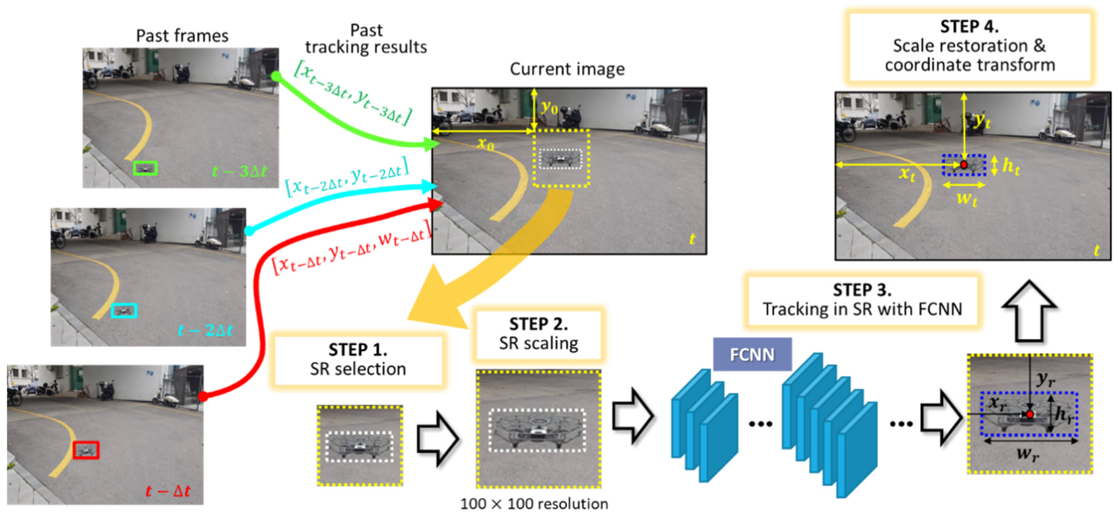
The proposed tracking algorithm comprises four steps, as shown in Figure 1. First, the location and size of the SR are obtained from the tracking results of previous frames. Second, the size of the SR is adjusted to a constant size (100 × 100). Next, the location and size of the object in the SR are estimated using FCNN. Finally, the tracking results of the SR are transformed, and the full image is obtained.
This SR-based tracker can accurately track objects with fast computation. First, the variations in the size and location of the target objects (in images) can increase the tracking error. The error is large if the object appears very small in the images. If the aspect ratio is extremely large or extremely small, accurate tracking becomes challenging. Second, tracking with full images requires a long computation time if the size of the image is large. Thus, an SR-based tracking model was developed and used instead of considering the full image.
The compact SR (CSR) tracker determines the current SR using the last tracking result only. Specifically, the center of the current SR was determined as the center of the object in the previous frame. The width and height of the current SR change depending on the object size in the previous frame. If the size of a target object (in images) remains constant over time, tracking can be very accurate and robust. In this study, the ratio of the SR width to the object width remained constant across several frames. However, this approach does not guarantee accurate and robust tracking. Thus, various strategies and methods have been developed to improve the quality of the SR.
2.1. Adaptive SR
To improve the tracking accuracy and robustness, some functions were included in the CSR model; these were shrink constraints (SC), size optimization (SO), and path prediction (PP).
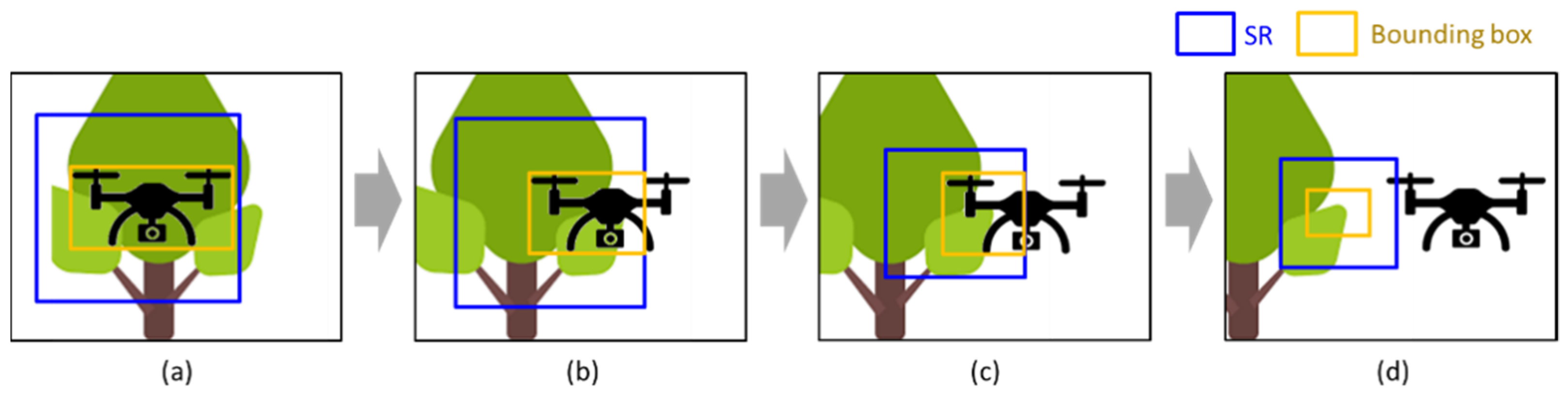
Shrink constraints: If a portion of a target object is truncated in the SR, this truncation can cause tracking failure. Then, the estimated size becomes smaller than the true size, as depicted in Figure 2. In the CSR model, the SR size was controlled to be linearly proportional to the object size. Thus, if the estimation result is smaller than the true size owing to truncation, as shown in Figure 2b, the size of the SR decreases in the following frame, as shown in Figure 2c. The SR continues to shrink in subsequent frames, which results in tracking failure, as shown in Figure 2d.
The SC of the SR was established to address this problem. First, the size of the SR is constrained to not be smaller than a threshold value. This constraint prevents the SR from shrinking beyond a certain size even if the object is truncated in the SR. Second, the size of the SR is constrained to not shrink if one or more edges of a bounding box are located on the edge of the SR in the previous frame. In the case of a moving object, when the image is cropped in the position of the previous frame, the object deviates from the center and is placed on the side. Finally, when the object is located near the edge of the SR, the shrinkage of the SR is inhibited. These schemes contribute to the robustness of the tracking algorithm.
Size optimization: As previously mentioned, SR size is determined such that the ratio of SR width to object width remains constant across all frames. The accuracy of the FCNN and the failure rate depend on this ratio. Thus, SO was conducted considering the performance of the tracking algorithm.
Path prediction: For the tracking of mobile objects, the location of the SR can be more accurately estimated when the dynamics of the objects are considered. Whereas CSR only considers the previous position of the object for determining the location of the current SR, the location of a trajectory predictive SR is determined based on the previous velocity of the object as well as its previous position. The PP model can determine the current location of the SR as
where is the time interval between adjacent frames. Position is a two-dimensional vector in the images, and is a correction coefficient that can be obtained by minimizing the tracking error. Because the position in the images is affected by the motions of the object as well as by the movements of the camera and distortion in the images, a correction coefficient has been included in Equation (1).
2.2. Fully Convolutional Neural Network
The proposed algorithm detects the object in the SR image, scaled to a 100 × 100 resolution. The FCNN is responsible for predicting a bounding box in the SR; the bounding box can be characterized by four variables, , where and are the offsets from the top left in the scaled SR and and represent the width and height of the object in the scaled SR, respectively. FCNN is composed of 15 convolutional layers and five max pooling layers, as listed in Table 1. It utilizes 3 × 3 convolutional filters based on VGG [15] and Darknet [11,12,13]. The number of convolutional filters is increased over the layers. Zero paddings were applied to convolutional layers to enhance the tracking performance when the object was close to the SR edge. All layer blocks (except the final layer) include batch normalization and LeakyReLu.
The images used for training FCNN were prepared by cropping the SR from the full image because FCNN tracks the object in the SR. The cropped regions for training the FCNN were randomly selected to induce robustness to variations in the size and location of the object in the image. Specifically, the ratio of the cropped region scale to the object size was randomly selected from a value between 1.2 and 1.7. The location of the cropped region is determined such that a 90% or higher portion of the target is contained in the cropped region. In addition, image rotation and color variation were also conducted to facilitate data augmentation.
The resulting model was trained using the following loss function.
where , , , and represent the estimated location and size, and , , , and are the true location and size. The Adam optimizer was used for training. The model was trained for 1000 epochs with a learning rate of 10−4. The model was implemented using the PyTorch 1.8.0 framework with Compute Unified Device Architecture (CUDA) 11.1. GeForce RTX 3090 GPU and Xeon Silver 4215R 3.20 GHz CPU were used for training and testing.
2.3. Scale Restoration and Coordinate Transform
Because FCNN conducts tracking in the SR, the tracking results from the SR have to be transformed to coordinates in the full image, as follows:
where , , , and are the tracking results in SR, and , , , and are the tracking results in the full image. Furthermore, and denote the coordinates of the left top of the SR in the full image, respectively; is the size of the scaled SR in the full image, and is the size prior to restoration (i.e., 100 pixels).
3. Dataset Description
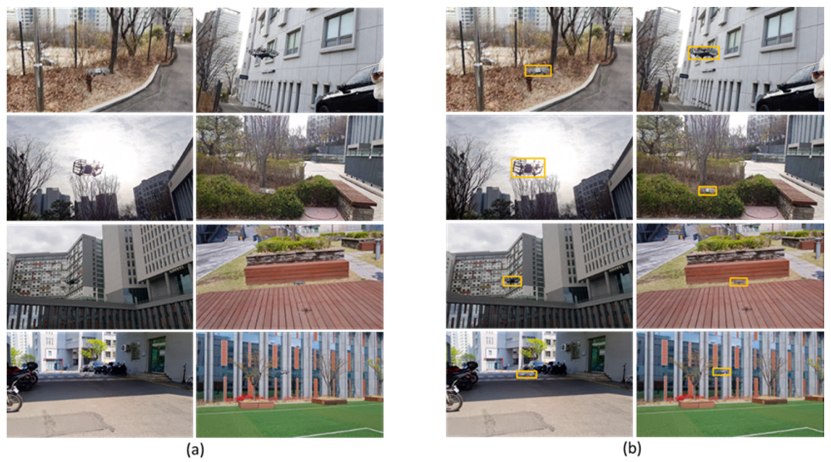
In this study, a MAV (DJI Tello) was selected as the target object because of the difficulty in tracking a small object that moves in various background scenes. Images (with 1280 × 720 resolution) of the flying MAV were recorded for training and testing. Figure 3a shows examples of the original dataset, and the bounding boxes of the MAV are shown in Figure 3b. The detection of the MAV in these images is challenging because of its small size and indistinguishable color from the background.
For accurate and robust tracking, the MAV was captured under various circumstances. For example, the background is complex and similar to the MAV in some images. In other images, the MAV is not fully visible because of backlight, or the MAV is blurred due to its rapid movement. The data are composed of three groups. Dataset1 is composed of 3585 images for training FCNN; Dataset2 comprises two sequences (451 and 499 frames) used for SO. This dataset is also used to obtain the coefficients for the PP model. Dataset3 comprises five sequences captured in various environments, whereby individual sequences are composed of 301–360 frames. This dataset is used to validate the performance of the tracking algorithm.
4. Results
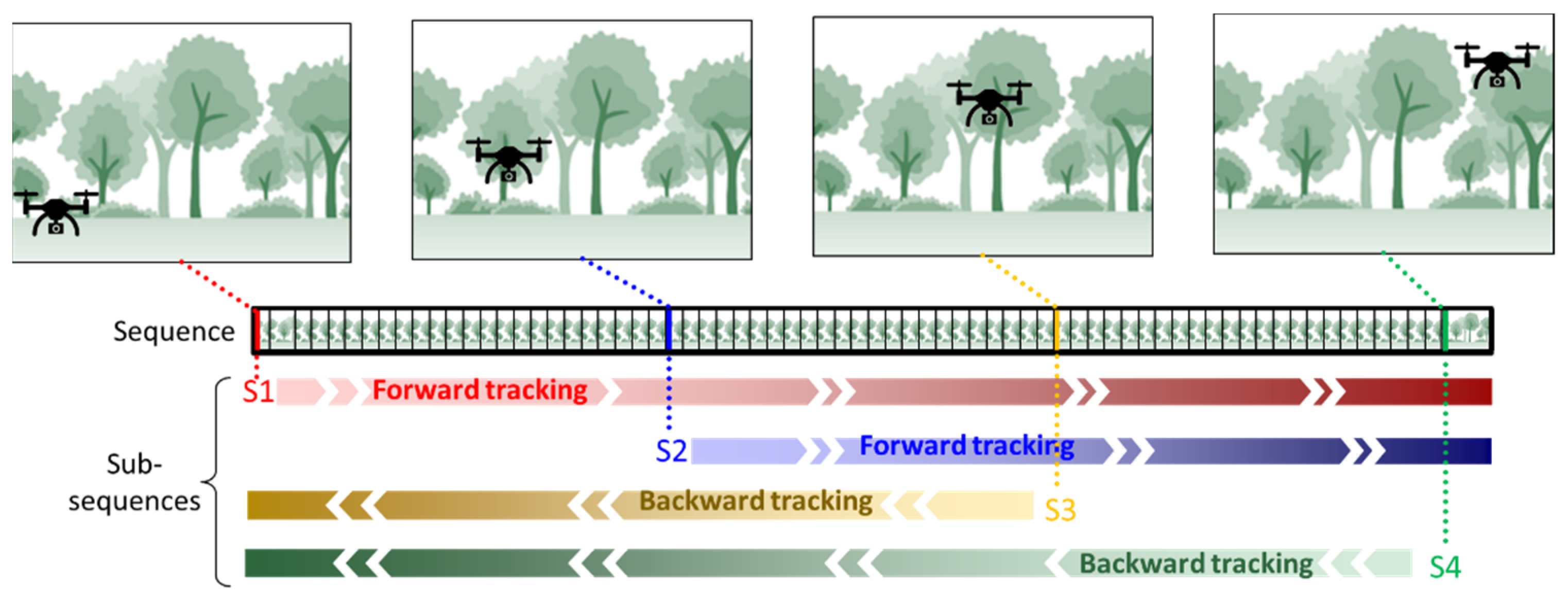
The tracking performance was evaluated in terms of accuracy, robustness, and the expected average overlap curve (EAOC) [33]. To calculate these performance indices, the starting points are selected every 50 frames. The algorithm then starts to track a target from each starting point to the final frame or initial frame, as shown in Figure 4. For example, S1 and S2 are closer to the initial frame than to the final frame. For these starting points, tracking is conducted in the forward direction. S3 and S4 are closer to the final frame; thus, backward tracking is performed. The group of frames from the starting point to the final (or initial) frame is called a sub-sequence.
The tracking accuracy for the kth starting point can be calculated as follows:
where is the number of frames before tracking failure occurs and IOU is the ratio of the intersected area to the union area of the estimated bounding box and the ground truth bounding box. The robustness of the kth starting point can be calculated as
where is the number of frames in a subsequence. Then, the total accuracy and robustness can be calculated by averaging and over the starting points and sequences.
The EAO curve represents both accuracy and robustness with extended sub-sequences. If tracking fails in the middle of a sub-sequence, the corresponding extended sub-sequence is constructed with the original images of the sub-sequence and dummy frames. Dummy frames are needed to calculate the EAOC, and tracking cannot be performed in dummy frames; that is, the IOU is zero in dummy frames. The number of dummy frames is determined such that the length of the extended sub-sequence is the same as that of the original sequence. If tracking is completed in the final frame without failure in another sub-sequence, the corresponding extended sub-sequence does not contain any dummy frames. The EAOC value can then be calculated as:
where represents the IOU value for the ith frame of the kth extended sub-sequence and is the number of extended sub-sequences that contain the ith frame. The ith frame can be either the original image or a dummy frame.
In the following section, the performances of the four trackers are compared. The first model is the CSR tracker; hereinafter, this model is referred to as CSR. The second model is constructed by applying the SC to the CSR model and is referred to as CSR + SC. The third model is created by adding the SO to the second model and is referred to as CSR + SP + SC. The last model includes PP in addition to the third model and is referred to as CSR + SP + SC + PP.
4.1. Effects of SC
The shrinkage of the SR was observed in the test using CSR. Figure 5a shows the SR when the MAV begins to be truncated at the right edge of the SR. Then, owing to the MAV motion, only half of the MAV is included in the SR, as shown in Figure 5b. Consequently, the size of the SR decreases further, and the tracker almost loses the MAV, as shown in Figure 5c. Tracking failure occurs in a few subsequent frames.
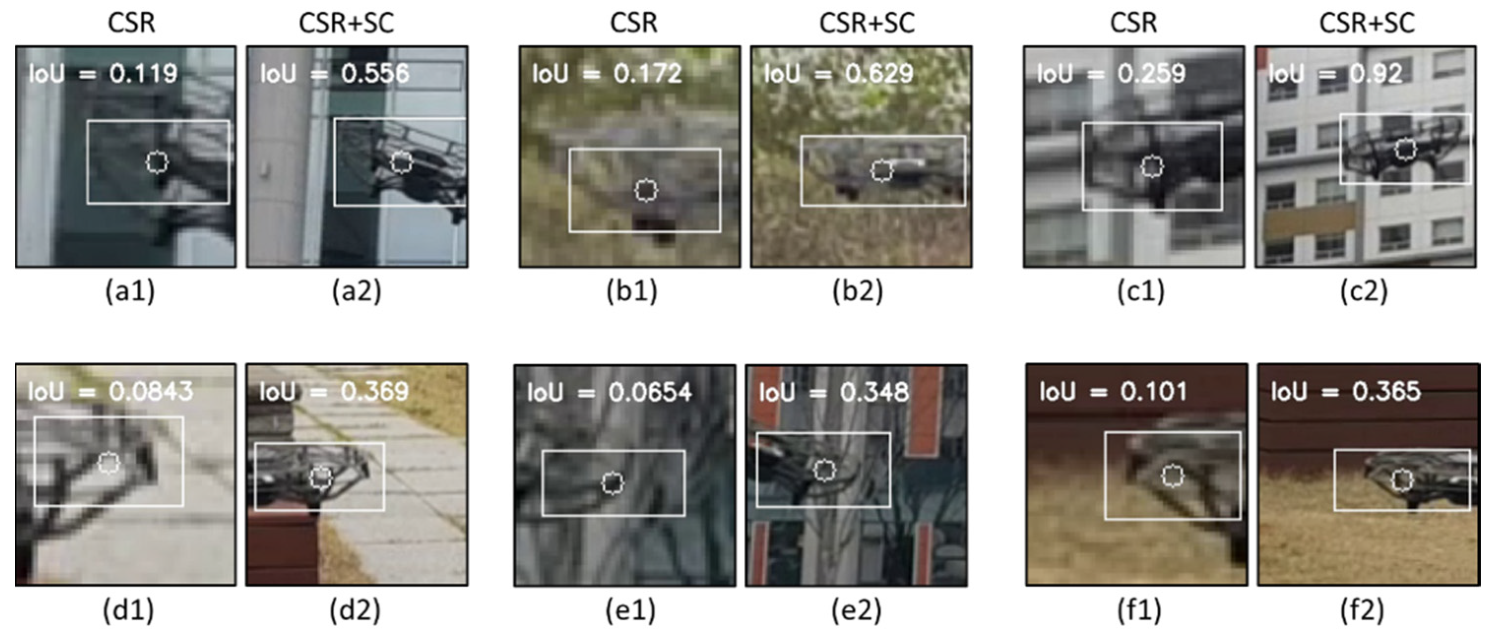
The SC prevents tracking failures caused by undesirable SR shrinkage. Figure 6 shows the SR and predicted bounding box in the absence and presence of SC in the same frame. Although the over-shrink preventive SR considerably increased the IOU value, a small truncation still remained. This limitation was resolved by SO and PP.
4.2. Optimization of SR Size
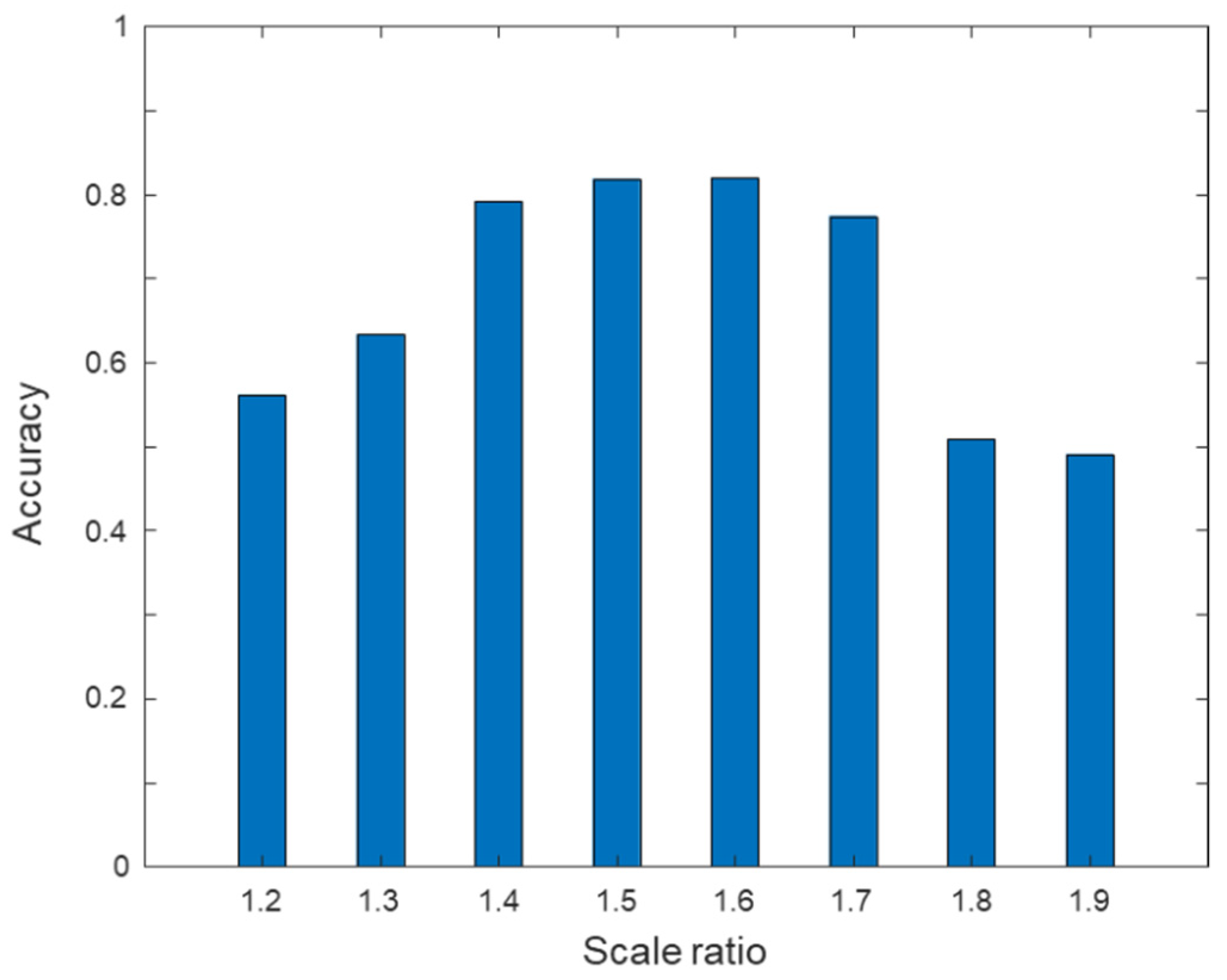
The size of the SR must be optimized to improve the tracking performance of the proposed method. If SR is extremely large compared to the size of the target object, other distracting objects can also be contained in the SR. Subsequently, the tracker may track other objects in the SR. If the SR is extremely small, the tracker is likely to lose moving objects. A constant value is selected for the scale ratio of the object and SR. Then, the size of the SR can be determined by multiplying the scale ratio by the object size of the previous frame. Because the object size in the current frame can be estimated after the current SR is determined in the online tracking, the object size in the previous frame should be used to determine the size of the current SR.
The effect of the scale ratio (of SR and target object) on the accuracy was investigated to determine the optimal size, as shown in Figure 7. These results were measured when truncation-preventive SR was applied. The tracking accuracy was at a maximum when the scale ratio is 1.4, 1.5, and 1.6. When the scale ratio was larger than 1.7, the accuracy considerably decreased because several other objects and large areas of the background were within the SR. Although truncation-preventive SR is applied, it cannot prevent all possibilities of truncation when the scale ratio is small. Thus, a rapidly moving object can be truncated in the SR when a small-scale ratio (i.e., 1.2) is used. Owing to this truncation, the accuracy decreases when the scale ratio is small. Inaccurate estimation of the target size results in an inappropriate SR size because the size of the SR is determined by the target size in the previous frame. Considering the accuracy, the optimal scale ratio is determined to be 1.6, which can vary depending on the target object because the value depends on the motion and shape features of the target object.
4.3. Path Predictive SR
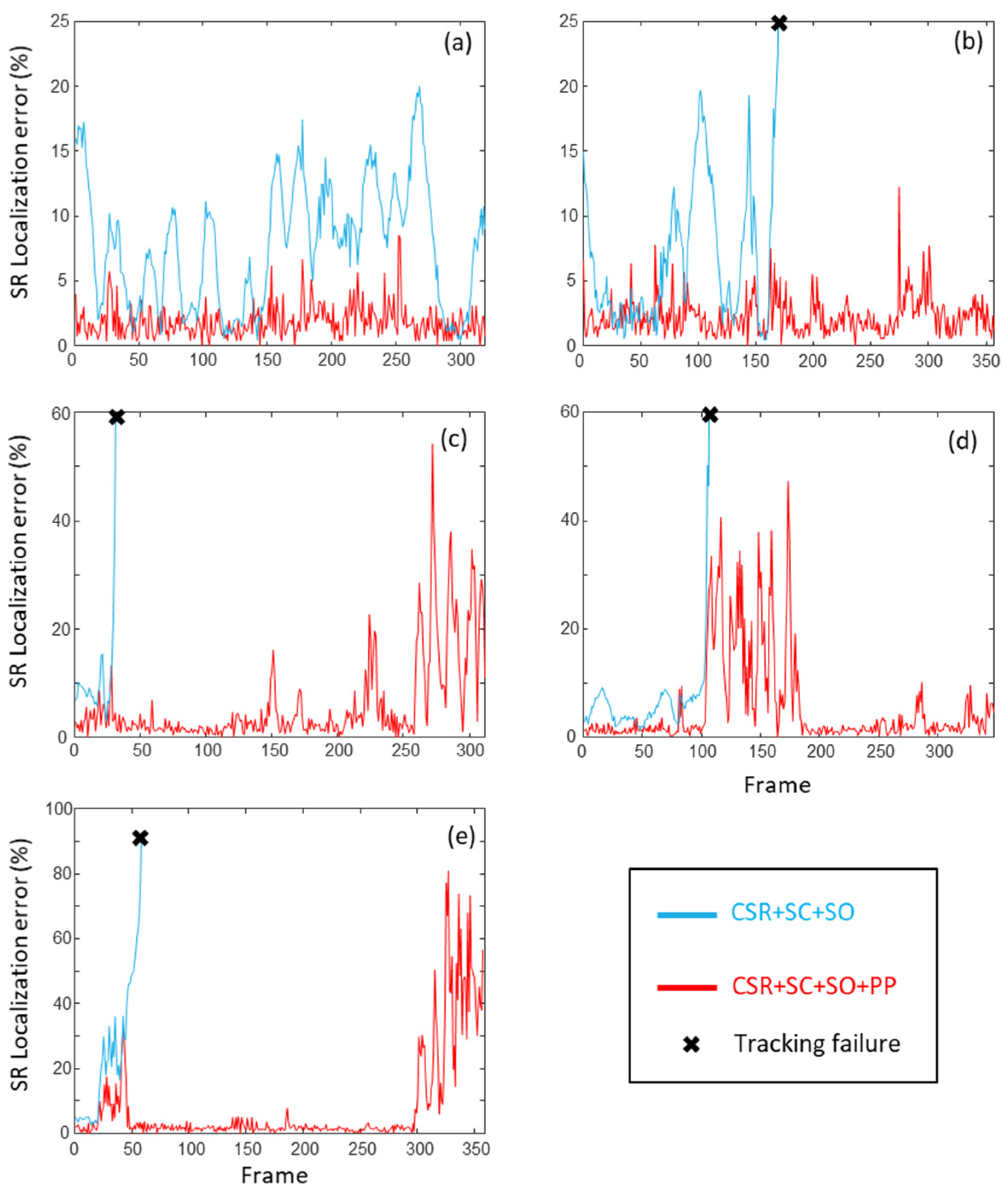
The PP model was generated by minimizing the location error of the SR in the sequences. To obtain the error, the distance (in pixels) between the center point of the SR and the true center point of the MAV was calculated. Then, the location error was calculated by dividing the distance by the size of the SR. The value of the correction coefficient in Equation (1) was determined to be 0.9836 by minimizing the constraint that should be greater than or equal to 0. The error in this minimization process is not a tracking error but is a location error of the SR. SC and SO were also adopted during the minimization of PP. The sequences used consisted of approximately 1000 frames (30 FPS).
The effects of PP were verified using test sequences. PP significantly reduced the SR localization error in most frames, as shown in Figure 8. Furthermore, large errors were observed frequently in the absence of PP; these large errors can cause tracking failure. However, PP treatment reduced the risk of failure by a remarkable amount. Thus, PP prevents the SR from losing the target object, and the robustness can be improved.
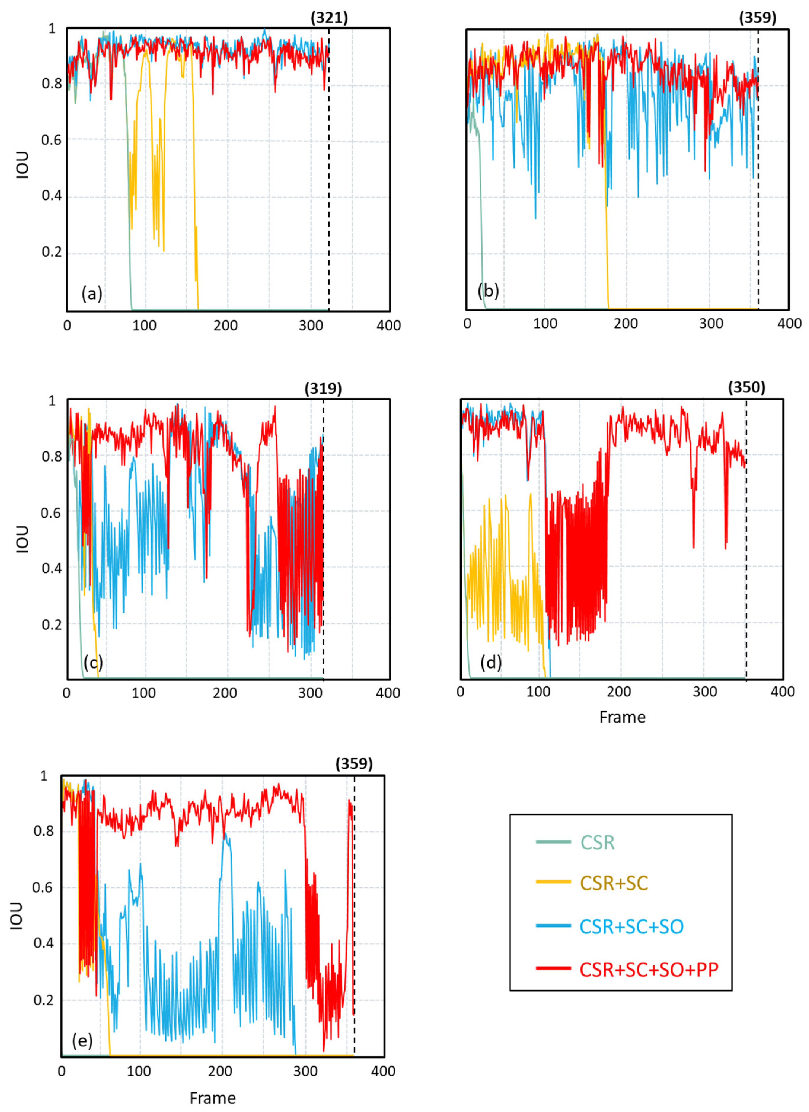
The tracking performance of the models was compared with the IOU values of the test sequences, as shown in Figure 9. CSR failed to track across 100 frames in each experiment. Specifically, it failed within 50 frames, except for sequence 1. CSR + SC tracked the MAV for longer than CSR did. However, it also failed at 100–150 frames, indicating the limitation of SC. Although CSR + SC + SO provided robust tracking, its IOU value (i.e., accuracy) fluctuated largely across the frames. PP resolves this unstable tracking. Except for some sections, the IOU of CSR + SC + SO + PP was maintained at a high level (i.e., 0.8–1).
PP can prevent tracking failure caused by the fast motions of the MAV. While the truncation from the SR can be prevented by SC for a slowly flying MAV, SC cannot prevent tracking failure if the MAV flies at a high speed. Specifically, when an MAV is truncated from the SR because of its fast motion, the CSR + SC model can prevent over-shrinkage. However, the error in the bounding box caused by truncation remains, as shown in Figure 5. The CSR + SC model determines the center of the SR in the following frame as the center of the current bounding box. Thus, if the target is stationary or moves slowly, this truncation can be removed. However, if the target moves fast, it is continuously truncated (or vanishes) from the SR, which can lead to tracking failure, as shown in Figure 9d,e. In contrast, when PP is applied, it moves the SR such that its center is close to the midpoint of the moving target. Thus, truncation and subsequent failure are prevented by PP. For example, in Figure 9d, failure did not occur even though the accuracy remained low for some frames.
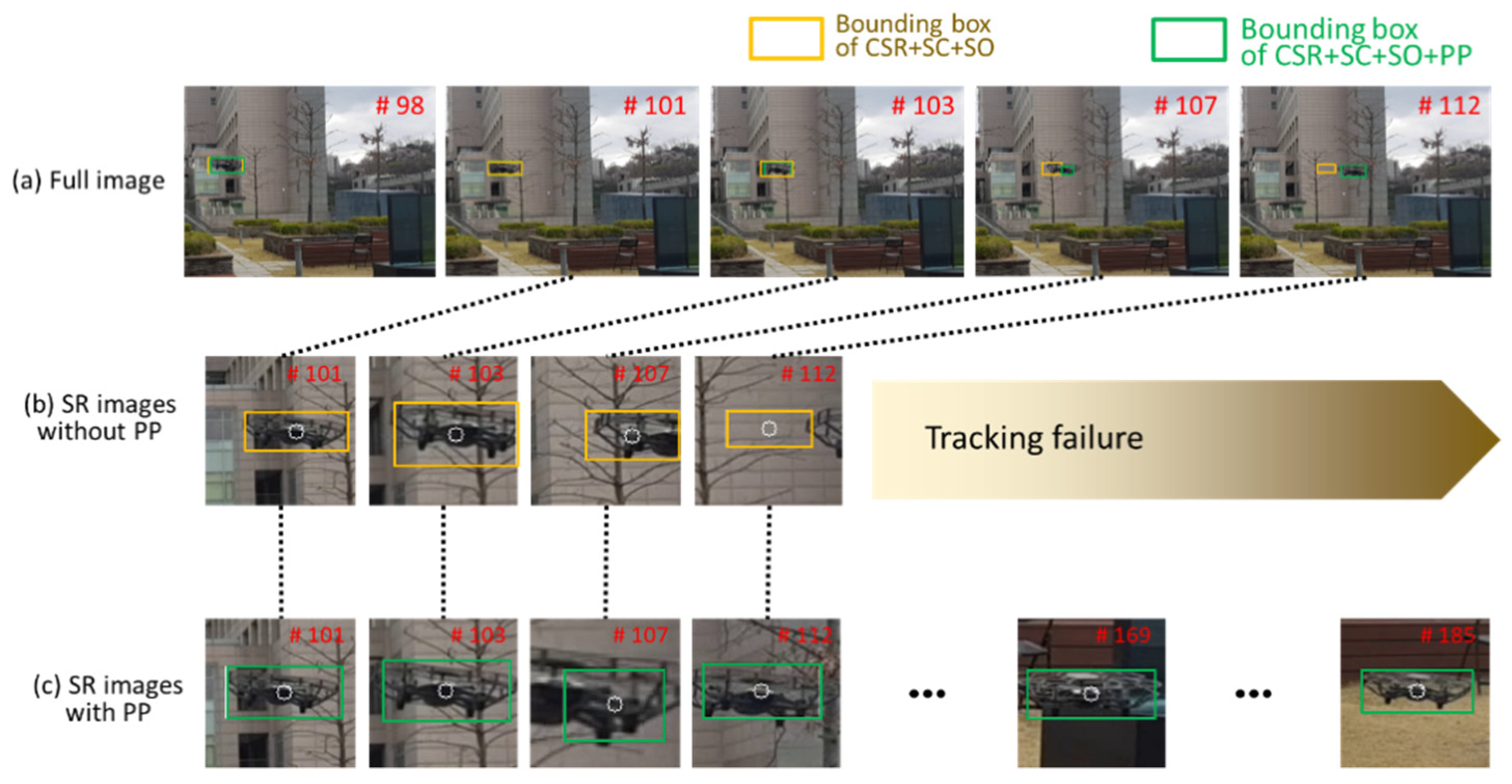
PP also provides opportunities for recovering high IOU values that decrease due to misinterpretations of the background in previous frames. For example, as shown in Figure 9d, the IOU started to significantly decrease for both the CSR + SC + SO and CSR + SC + SO + MP models at the 114th frame. The background is very similar to the MAV in this frame. While the CSR + SC + SO model suddenly fails after this frame, PP prevents the tracker from failing. Although the IOU value remains low for a long interval owing to the distracting background, PP enables the SR to follow the MAV. Afterward, when the background is changed to be less similar to the MAV, the IOU value increases to a high level (i.e., 0.8–1). A series of images and tracking results of the accuracy recovery function are shown in Figure 10. While the CSR + SC + SO model failed to track from the 112th frame onwards, PP maintained tracking and returned to a high estimation state after 73 frames. A Supplementary Materials (movie file) shows the tracking performance of the CSR + SC + SO + PP model.
4.4. Performance Evaluation
The performance of the models was quantitatively compared in terms of accuracy, robustness, and EAOC of the test sequences. The results of the accuracy and robustness are listed in Table 2. CSR exhibited an accuracy of 0.613 and a robustness of 0.086. The accuracy of CSR is satisfactory. However, this accuracy is valid only under easily trackable conditions; in extreme conditions, CSR fails rapidly, and this failure is not considered in the calculations of the accuracy. In contrast, the robustness is low because of frequent truncations and subsequent failures. In the absence of SC and PP, SR can lose the MAV even if it moves slowly.
SC exhibits a significantly improved robustness of 0.583. In contrast, the increase in accuracy by SC is negligible because the truncation of the target in SR cannot be corrected by SC. The optimization of SR size improves both accuracy and robustness. Although PP slightly reduces the accuracy, it significantly increases the robustness. This suggests that PP is necessary for the reliable tracking of dynamically moving targets.
To verify the performance of the proposed model, tracking was also conducted with another recent tracker (i.e., Ocean [34]). This tracker was used for benchmarking because they achieved high scores in VOT 2018 and 2019. This model was fine-tuned using Dataset1, which was used in this study. The dataset was resized to fit the original dataset, and the trackers were trained for 500 epochs, which is sufficiently large considering the epoch numbers used in previous studies. The proposed model achieved similar or higher accuracy and robustness compared to this previous tracker, as shown in Table 2.
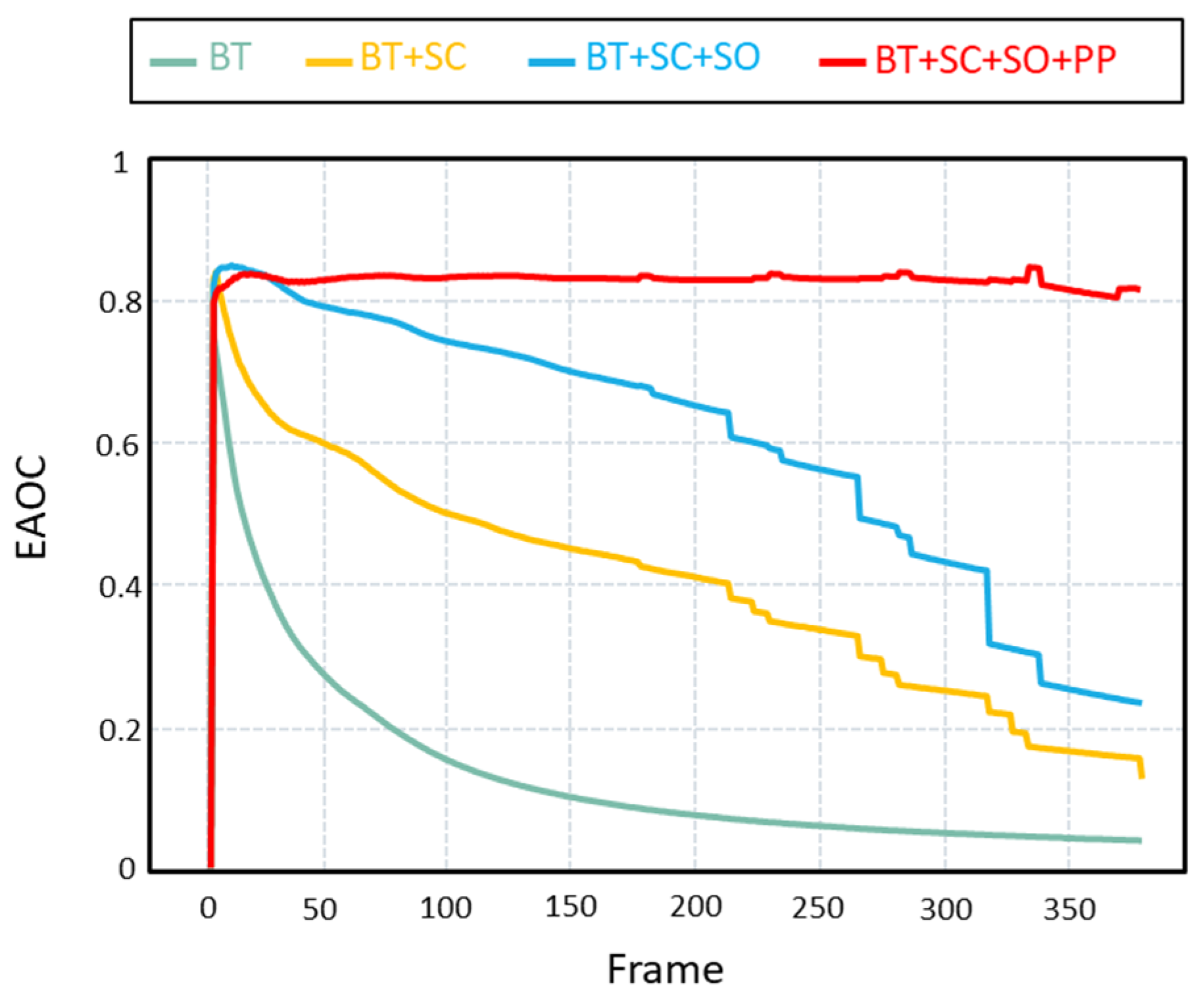
The effects of SC, SO, and PP can also be evaluated using EAOC. If the EAOC value is high for a frame, accurate tracking is achieved, and failure does not occur in most frames of that sequence. Owing to early failure, the EAOC of the CSR noticeably decreases across the frames, as shown in Figure 11. Although SC and SO have an increased EAOC value, the value is low after 300 frames. In contrast, the EAOC value remains high when PP is applied, which suggests that PP is necessary for long tracking tasks.
Among the four models used in this study, CSR + TP + SO + PP is the most accurate and reliable model for tracking. Thus, the inference time of the model was measured. When GeForce RTX 3090 GPU and Xeon Silver 4215R 3.20 GHz CPU were used for inference, the computation time was approximately 24 ms per frame (i.e., 410 FPS). This computation speed suggests that the model can be used for real-time tracking.
5. Conclusions
In this study, an SR-based MAV tracker was developed by integrating several methods to improve tracking accuracy, robustness, and computation speed. First, SC reduces the probability of losing the target from the SR. Second, SO optimizes the SR size by considering the effects of the SR size on the tracking accuracy. Finally, PP estimates a more accurate location of the SR by considering the target object motion. Although SC, SO, and PP were conducted with simple and existing operations, the combination of these methods led to significant tracking improvements (i.e., accuracy, robustness, and EAOC). Moreover, the proposed tracker can be applied to real-time tracking because of its high computation speed (410 FPS). Furthermore, the proposed tracker shows higher accuracy and robustness than a tracker named Ocean, which is one of the high-end trackers in the test dataset used in this study.
Although the proposed model exhibits satisfactory tracking performance, additional work is required to address its limitations. First, the proposed tracker was verified using only an MAV. For use in other applications, its performance must be tested with other objects. Second, the proposed model must be updated to manage occlusion periods. When the target size is reduced by occlusion, the SR size can also decrease, which can lead to inaccurate tracking. Thus, an occlusion-detectable model should be developed. In the worst case, the target can be fully covered by other objects. Object detection algorithms can be modified to address this problem. In addition, the tracker should be updated using multiple SRs for multiple-object tracking.
Supplementary Materials
The following are available online at https://www.mdpi.com/article/10.3390/app11167741/s1, Video S1: MAV-tracker.
Author Contributions
Conceptualization, W.N.; methodology, W.P.; software, W.P.; validation, W.P.; formal analysis, D.L.; investigation, W.P.; resources, W.P.; data curation, J.Y.; writing—original draft preparation, W.P.; writing—review and editing, W.N.; visualization, W.P.; supervision, W.N.; project administration, W.N.; funding acquisition, W.N. All authors have read and agreed to the published version of the manuscript.
Funding
This research was supported by the National Research Foundation of Korea (NRF) grant funded by the Korea government (MSIT) (No. 2021R1F1A1063463) and the Chung-Ang University Research Scholarship Grants in 2019.
Conflicts of Interest
The authors declare no conflict of interest.
References
- Wang, L.; Ouyang, W.; Wang, X.; Lu, H. Visual tracking with fully convolutional networks. In Proceedings of the IEEE International Conference On Computer Vision, Santiago, Chile, 13–16 December 2015; pp. 3119–3127. [Google Scholar]
- Krizhevsky, A.; Sutskever, I.; Hinton, G.E. Imagenet classification with deep convolutional neural networks. Adv. Neural Inf. Process. Syst. 2012, 25, 1097–1105. [Google Scholar] [CrossRef]
- He, K.; Zhang, X.; Ren, S.; Sun, J. Deep residual learning for image recognition. In Proceedings of the IEEE Conference on Computer Vision and Pattern Recognition, Las Vegas, NV, USA, 27–30 June 2016; pp. 770–778. [Google Scholar]
- Felzenszwalb, P.F.; Girshick, R.B.; McAllester, D.; Ramanan, D. Object detection with discriminatively trained part-based models. IEEE Trans. Pattern Anal. Mach. Intell. 2009, 32, 1627–1645. [Google Scholar] [CrossRef] [PubMed] [Green Version]
- Girshick, R.; Donahue, J.; Darrell, T.; Malik, J. Rich feature hierarchies for accurate object detection and semantic segmentation. In Proceedings of the IEEE Conference on Computer Vision and Pattern Recognition, Columbus, OH, USA, 23–28 June 2014; pp. 580–587. [Google Scholar]
- Girshick, R.; Donahue, J.; Darrell, T.; Malik, J. Region-based convolutional networks for accurate object detection and segmentation. IEEE Trans. Pattern Anal. Mach. Intell. 2015, 38, 142–158. [Google Scholar] [CrossRef] [PubMed]
- Girshick, R. Fast r-cnn. In Proceedings of the IEEE International Conference on Computer Vision, Santiago, Chile, 13–16 December 2015; pp. 1440–1448. [Google Scholar]
- Ren, S.; He, K.; Girshick, R.; Sun, J. Faster R-CNN: Towards real-time object detection with region proposal networks. IEEE Trans. Pattern Anal. Mach. Intell. 2016, 39, 1137–1149. [Google Scholar] [CrossRef] [PubMed] [Green Version]
- He, K.; Gkioxari, G.; Dollár, P.; Girshick, R. Mask r-cnn. In Proceedings of the IEEE International Conference on Computer Vision, Santiago, Chile, 13–16 December 2015; pp. 2961–2969. [Google Scholar]
- Dai, J.; Li, Y.; He, K.; Sun, J. R-fcn: Object detection via region-based fully convolutional networks. arXiv 2016, arXiv:1605.06409. [Google Scholar]
- Redmon, J.; Divvala, S.; Girshick, R.; Farhadi, A. You only look once: Unified, real-time object detection. In Proceedings of the IEEE Conference on Computer Vision and Pattern Recognition, Las Vegas, NV, USA, 27–30 June 2016; pp. 779–788. [Google Scholar]
- Redmon, J.; Farhadi, A. YOLO9000: Better, faster, stronger. In Proceedings of the IEEE Conference on Computer Vision and Pattern Recognition, Honolulu, HI, USA, 21–26 July 2017; pp. 7263–7271. [Google Scholar]
- Redmon, J.; Farhadi, A. Yolov3: An incremental improvement. arXiv 2018, arXiv:1804.02767. [Google Scholar]
- Liu, W.; Anguelov, D.; Erhan, D.; Szegedy, C.; Reed, S.; Fu, C.-Y.; Berg, A.C. Ssd: Single shot multibox detector. In Proceedings of the European Conference on Computer Vision, Amsterdam, The Netherlands, 11–14 October 2016; pp. 21–37. [Google Scholar]
- Simonyan, K.; Zisserman, A. Very deep convolutional networks for large-scale image recognition. arXiv 2014, arXiv:1409.1556. [Google Scholar]
- Szegedy, C.; Liu, W.; Jia, Y.; Sermanet, P.; Reed, S.; Anguelov, D.; Erhan, D.; Vanhoucke, V.; Rabinovich, A. Going deeper with convolutions. In Proceedings of the IEEE Conference on Computer Vision and Pattern Recognition, Boston, MA, USA, 7–12 June 2015; pp. 1–9. [Google Scholar]
- Zhong, Y.; Wang, J.; Peng, J.; Zhang, L. Anchor box optimization for object detection. In Proceedings of the IEEE/CVF Winter Conference on Applications of Computer Vision, Snowmass Village, CO, USA, 1–5 March 2020; pp. 1286–1294. [Google Scholar]
- Lin, T.-Y.; Dollár, P.; Girshick, R.; He, K.; Hariharan, B.; Belongie, S. Feature pyramid networks for object detection. In Proceedings of the IEEE Conference on Computer Vision and Pattern Recognition, Honolulu, HI, USA, 21–26 July 2017; pp. 2117–2125. [Google Scholar]
- Reddy, K.R.; Priya, K.H.; Neelima, N. Object Detection and Tracking—A Survey. In Proceedings of the 2015 International Conference on Computational Intelligence and Communication Networks (CICN), Jabalpur, India, 12–14 December 2015; pp. 418–421. [Google Scholar]
- Ciaparrone, G.; Sánchez, F.L.; Tabik, S.; Troiano, L.; Tagliaferri, R.; Herrera, F. Deep learning in video multi-object tracking: A survey. Neurocomputing 2020, 381, 61–88. [Google Scholar] [CrossRef] [Green Version]
- Li, P.; Wang, D.; Wang, L.; Lu, H. Deep visual tracking: Review and experimental comparison. Pattern Recognit. 2018, 76, 323–338. [Google Scholar] [CrossRef]
- Kumar, B.V. Minimum-variance synthetic discriminant functions. JOSA A 1986, 3, 1579–1584. [Google Scholar] [CrossRef]
- Mahalanobis, A.; Kumar, B.V.; Casasent, D. Minimum average correlation energy filters. Appl. Opt. 1987, 26, 3633–3640. [Google Scholar] [CrossRef] [PubMed]
- Bolme, D.S.; Beveridge, J.R.; Draper, B.A.; Lui, Y.M. Visual object tracking using adaptive correlation filter. In Proceedings of the 2010 IEEE Computer Society Conference on Computer Vision and Pattern Recognition, San Francisco, CA, USA, 13–18 June 2010; pp. 2544–2550. [Google Scholar]
- Henriques, J.F.; Caseiro, R.; Martins, P.; Batista, J. High-speed tracking with kernelized correlation filters. IEEE Trans. Pattern Anal. Mach. Intell. 2014, 37, 583–596. [Google Scholar] [CrossRef] [PubMed] [Green Version]
- Danelljan, M.; Robinson, A.; Khan, F.S.; Felsberg, M. Beyond correlation filters: Learning continuous convolution operators for visual tracking. In Proceedings of the European Conference on Computer Vision, Amsterdam, The Netherlands, 11–14 October 2016; pp. 472–488. [Google Scholar]
- Danelljan, M.; Bhat, G.; Shahbaz Khan, F.; Felsberg, M. Eco: Efficient convolution operators for tracking. In Proceedings of the IEEE Conference on Computer Vision and Pattern Recognition, Honolulu, HI, USA, 21–26 July 2017; pp. 6638–6646. [Google Scholar]
- Nam, H.; Han, B. Learning multi-domain convolutional neural networks for visual tracking. In Proceedings of the IEEE Conference on Computer Vision and Pattern Recognition, Las Vegas, NV, USA, 27–30 June 2016; pp. 4293–4302. [Google Scholar]
- Danelljan, M.; Bhat, G.; Khan, F.S.; Felsberg, M. Atom: Accurate tracking by overlap maximization. In Proceedings of the IEEE/CVF Conference on Computer Vision and Pattern Recognition, Long Beach, CA, USA, 15–20 June 2019; pp. 4660–4669. [Google Scholar]
- Bertinetto, L.; Valmadre, J.; Henriques, J.F.; Vedaldi, A.; Torr, P.H. Fully-convolutional siamese networks for object tracking. In Proceedings of the European Conference on Computer Vision, Amsterdam, The Netherlands, 8–10 and 15–16 October 2016; pp. 850–865. [Google Scholar]
- Li, B.; Yan, J.; Wu, W.; Zhu, Z.; Hu, X. High performance visual tracking with siamese region proposal network. In Proceedings of the IEEE Conference on Computer Vision and Pattern Recognition, Salt Lake City, UT, USA, 18–23 June 2018; pp. 8971–8980. [Google Scholar]
- Guo, D.; Wang, J.; Cui, Y.; Wang, Z.; Chen, S. SiamCAR: Siamese fully convolutional classification and regression for visual tracking. In Proceedings of the IEEE/CVF Conference on Computer Vision and Pattern Recognition, Seattle, WA, USA, 13–19 June 2020; pp. 6269–6277. [Google Scholar]
- Kristan, M.; Leonardis, A.; Matas, J.; Felsberg, M.; Pflugfelder, R.; Kämäräinen, J.-K.; Danelljan, M.; Zajc, L.Č.; Lukežič, A.; Drbohlav, O.; et al. The eighth visual object tracking VOT2020 challenge results. In Proceedings of the European Conference on Computer Vision, Glasgow, UK, 23–28 August 2020; pp. 547–601. [Google Scholar]
- Zhang, Z.; Peng, H.; Fu, J.; Li, B.; Hu, W. Ocean: Object-aware anchor-free tracking. In Proceedings of the Computer Vision–ECCV 2020: 16th European Conference, Glasgow, UK, 23–28 August 2020; pp. 771–787. [Google Scholar]
Figure 1.
Procedure of tracking with search region (SR).

Figure 2.
SR shrinkage caused by truncation. The blue box represents the SR, and the yellow box represents the tracking result calculated with a fully convolutional neural network (FCNN). (a–d) show sequential frames.
Figure 2.
SR shrinkage caused by truncation. The blue box represents the SR, and the yellow box represents the tracking result calculated with a fully convolutional neural network (FCNN). (a–d) show sequential frames.

Figure 3.
Dataset samples of flying MAV in various backgrounds. (a) original images, and (b) same images with annotated bounding boxes of the MAV.
Figure 3.
Dataset samples of flying MAV in various backgrounds. (a) original images, and (b) same images with annotated bounding boxes of the MAV.

Figure 4.
Starting points and tracking direction for evaluation.

Figure 5.
Shrinkage of SR in the CSR tracker. (a–c) are the SR images in the sequential frames. The white box is the bounding box estimated by the FCNN.
Figure 5.
Shrinkage of SR in the CSR tracker. (a–c) are the SR images in the sequential frames. The white box is the bounding box estimated by the FCNN.

Figure 6.
Effects of SC on the truncation in SRs. (a1–f1) represent the SR of the CSR tracker; (a2–f2) show the SR when truncation preventive SR is applied.
Figure 6.
Effects of SC on the truncation in SRs. (a1–f1) represent the SR of the CSR tracker; (a2–f2) show the SR when truncation preventive SR is applied.

Figure 7.
Effects of scale ratio on accuracy.

Figure 8.
Localization error of SR across frames in the test sequences. (a–e) represent the error of test sequence 1–5, respectively.
Figure 8.
Localization error of SR across frames in the test sequences. (a–e) represent the error of test sequence 1–5, respectively.

Figure 9.
IOU values of the test sequences. Numbers in parenthesis represent the number of frames in the sequences. (a–e) represent the IOU values of test sequence 1–5, respectively.
Figure 9.
IOU values of the test sequences. Numbers in parenthesis represent the number of frames in the sequences. (a–e) represent the IOU values of test sequence 1–5, respectively.

Figure 10.
Recovery example of PP.

Figure 11.
EAOC of tracking models.


Table 1.
Structure of FCNN.
| Type | Number of CNN Filters | Size/Stride | Output Size |
|---|---|---|---|
| Convolutional layer | 16 | 3 × 3/1 | 100 × 100 |
| Convolutional layer | 32 | 3 × 3/1 | 100 × 100 |
| Convolutional layer | 16 | 3 × 3/1 | 100 × 100 |
| Convolutional layer | 32 | 3 × 3/1 | 100 × 100 |
| Max pooling layer | - | 2 × 2/2 | 50 × 50 |
| Convolutional layer | 16 | 3 × 3/1 | 50 × 50 |
| Convolutional layer | 8 | 3 × 3/1 | 50 × 50 |
| Convolutional layer | 16 | 3 × 3/1 | 50 × 50 |
| Max pooling layer | 2 × 2/2 | 25 × 25 | |
| Convolutional layer | 32 | 3 × 3/1 | 25 × 25 |
| Convolutional layer | 64 | 3 × 3/1 | 25 × 25 |
| Max pooling layer | - | 2 × 2/2 | 12 × 12 |
| Convolutional layer | 128 | 3 × 3/1 | 12 × 12 |
| Convolutional layer | 64 | 3 × 3/1 | 12 × 12 |
| Max pooling layer | - | 2 × 2/2 | 6 × 6 |
| Convolutional layer | 128 | 3 × 3/1 | 6 × 6 |
| Convolutional layer | 256 | 3 × 3/1 | 6 × 6 |
| Convolutional layer | 128 | 3 × 3/1 | 6 × 6 |
| Max pooling layer | - | 2 × 2/2 | 3 × 3 |
| Convolutional layer | 4 | 3 × 3/3 | 1 × 1 |
Table 2.
Tracking performance comparison.
| Method | Accuracy | Robustness |
|---|---|---|
| CSR | 0.613 | 0.086 |
| CSR + SC | 0.632 | 0.583 |
| CSR + SC + SO | 0.846 | 0.685 |
| CSR + SC + SO + PP | 0.811 | 1.0 |
| Ocean | 0.756 | 1.0 |
Publisher’s Note: MDPI stays neutral with regard to jurisdictional claims in published maps and institutional affiliations. |
© 2021 by the authors. Licensee MDPI, Basel, Switzerland. This article is an open access article distributed under the terms and conditions of the Creative Commons Attribution (CC BY) license (https://creativecommons.org/licenses/by/4.0/).
Share and Cite
MDPI and ACS Style
Park, W.; Lee, D.; Yi, J.; Nam, W. Visual MAV Tracker with Adaptive Search Region. Appl. Sci. 2021, 11, 7741. https://doi.org/10.3390/app11167741
AMA Style
Park W, Lee D, Yi J, Nam W. Visual MAV Tracker with Adaptive Search Region. Applied Sciences. 2021; 11(16):7741. https://doi.org/10.3390/app11167741
Chicago/Turabian StylePark, Wooryong, Donghee Lee, Junhak Yi, and Woochul Nam. 2021. "Visual MAV Tracker with Adaptive Search Region" Applied Sciences 11, no. 16: 7741. https://doi.org/10.3390/app11167741
Note that from the first issue of 2016, this journal uses article numbers instead of page numbers. See further details here.