Article

Multivariate Analysis Applied to Aquifer Hydrogeochemical Evaluation: A Case Study in the Coastal Significant Subterranean Water Body between “Cecina River and San Vincenzo”, Tuscany (Italy)

by
Alessia Bastianoni
1,2,
Enrico Guastaldi
2,3,*,
Alessio Barbagli
2,3,4,
Stefano Bernardinetti
2,3,
Andrea Zirulia
2,3,
Mariantonietta Brancale
2,3 and
Tommaso Colonna
2,3
1
Institute of Earth Sciences, Central University of Venezuela, Ciudad Universitaria de Caracas, Caracas 1083, Venezuela
2
CGT Center for GeoTechnologies, University of Siena, Via Vetri Vecchi, 34-52027 San Giovanni Valdarno, Italy
3
GEOexplorer Impresa Sociale S.r.l., Via E. Vezzosi, 15-52100 Arezzo, Italy
4
Department of Physics and Earth Science, University of Ferrara, Via Saragat, 1-44122 Ferrara, Italy
*
Author to whom correspondence should be addressed.
Appl. Sci. 2021, 11(16), 7595; https://doi.org/10.3390/app11167595
Submission received: 15 July 2021 / Revised: 10 August 2021 / Accepted: 12 August 2021 / Published: 18 August 2021
(This article belongs to the Special Issue Water Footprint and Life Cycle Assessment)

Abstract

:
The hydrogeochemical characteristics of the significant subterranean water body between “Cecina River and San Vincenzo” (Italy) was evaluated using multivariate statistical analysis methods, like principal component analysis and self-organizing maps (SOMs), with the objective to study the spatiotemporal relationships of the aquifer. The dataset used consisted of the chemical composition of groundwater samples collected between 2010 and 2018 at 16 wells distributed across the whole aquifer. For these wells, all major ions were determined. A self-organizing map of 4 × 8 was constructed to evaluate spatiotemporal changes in the water body. After SOM clustering, we obtained three clusters that successfully grouped all data with similar chemical characteristics. These clusters can be viewed to reflect the presence of three water types: (i) Cluster 1: low salinity/mixed waters; (ii) Cluster 2: high salinity waters; and (iii) Cluster 3: low salinity/fresh waters. Results showed that the major ions had the greater influence over the groundwater chemistry, and the difference in their concentrations allowed the definition of three clusters among the obtained SOM. Temporal changes in cluster assignment were only observed in two wells, located in areas more susceptible to changes in the water table levels, and therefore, hydrodynamic conditions. The result of the SOM clustering was also displayed using the classical hydrochemical approach of the Piper plot. It was observed that these changes were not as easily identified when the raw data were used. The spatial display of the clustering results, allowed the evaluation in a hydrogeological context in a quick and cost-effective way. Thus, our approach can be used to quickly analyze large datasets, suggest recharge areas, and recognize spatiotemporal patterns.

1. Introduction

Groundwater represents nearly 30% of the global water resources and is considered the most important resource of freshwater to the planet [1]. As such, it needs to be carefully monitored in order to determine as soon as possible any changes in its chemical composition and quality. In a climate change scenario, where a decrease in the amount and frequency of precipitation is taking place [2], it is paramount the implementation of cost-effective and simple techniques that allow a clear and quick detection of changes in the chemical characteristics of water resources, in particular for changes that can help understand the stress condition of an exploited resource.
Determining chemical and physical characteristics of groundwater allows an accurate and reliable classification of water bodies, usually through the trilinear plots proposed by [3,4], as suggested by [5]. These plots also allow the evaluation of hydrochemical processes; however, as [6] acknowledges, the identification of clear boundaries between categories is not easy, and since the transitions between each water type are smooth, most of the times no clear distinction between the water types is possible. From the last 12 years, several research groups (e.g., [6,7,8,9,10,11,12]) have tackled this issue applying multivariate statistics as a way to better evaluate spatial and temporal variability of the hydrogeochemical characteristics of groundwater. The most commonly used multivariate techniques are principal component analysis (PCA) and hierarchical clustering, since both allow the individuation and grouping of the main variables controlling the chemical composition of the waters. Recently, there’s also been an increasing trend to use self-organizing maps (SOMs, a type of artificial neural networks) to explore the spatial patterns of different water quality parameters when large data-sets are used and regional trends are of interest (e.g., [6,7,8,9,13]).
In 2010, the Tuscany Region authority (Italy) defined a series of “significative subterranean water bodies” (SSWBs) so as to protect the water resources hosted in these water bodies and undertake remediation/reclamation actions if needed [14]. Following this, the Agency for Environment Protection of the Tuscany Region has made available on the regional system of environmental information website the results of the physicochemical monitoring of all the wells distributed throughout the region. Thus, a massive amount of data (from 1968 until 2019) is available for analysis, although in most cases fragmented and in a non-harmonious way [6].
The SSWB of Cecina Valley is a coastal aquifer that comprises the sedimentary coastal plain of Cecina town where the Cecina River flows into the Ligurian Sea, and the area between Cecina town and San Vincenzo village. Two out of the three water bodies embedded in the Cecina Valley aquifer face important saline water intrusion issues. A situation also enhanced by the lowering of the piezometric level near Cecina town, and between Marina di Bibbona and Castagneto Carducci villages due to excessive water abstraction, particularly during the high-touristic summer periods [14].
As reported by [2,15], the Cecina Valley area will likely experience a considerable reduction in total precipitations as well as an increase in temperatures, shifting from a semi-arid climate to a more arid one [16]. This change could also have a negative influence over the hydrodynamics and hydrogeochemistry of this SSWB, since acknowledge infiltration of rainfall is the main recharge source for this aquifer [14].
Thus, the objectives of this study were: (i) identification of the source of recharge to the aquifers in the SSWB of Cecina Valley; (ii) recognition of spatial and temporal patterns in the hydrogeochemistry of the groundwater sampled by a combination of self-organizing maps and clustering analysis; and (iii) to interpret the natural processes and their influence on the spatial variations in water chemistry.

2. Materials and Methods

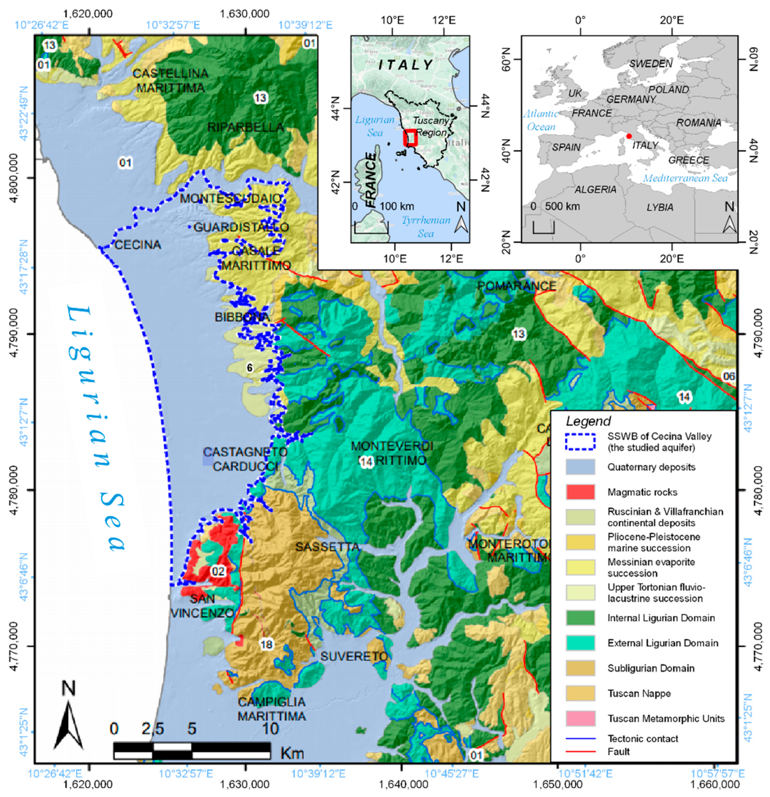
2.1. Geological and Hydrogeological Setting

The “Coastal Aquifer between Cecina River and San Vincenzo” SSWB is located in Livorno province of Tuscany, central Italy (Figure 1). The annual cumulative precipitation is nearly 700 mm and the main rivers draining the area are rivers Fine and Cecina, which drain the north and south areas respectively. This area is also densely populated and subjected to a high demand of drinkable water, especially during the summer [14] when the area inhabitants greatly increase due to tourism.
The SSWB studied is constituted by quaternary deposits (Figure 1) formed as a sequence of permeable gravel and sand layer (k ≅ 10−2 m/s) separated by impermeable silty-clayey deposits. The bedrock of this sequence is represented by: (i) the sands and clays with Arctica islandica (Linnaeus, 1767) in the northern part of the study area; (ii) the low-permeability Ligurian units in the southern part; and (iii) clayey deposits of uncertain stratigraphic position in the area between the Cecina River and Bolgheri village. The hydraulic head of this coastal water body appears to be consistent to the ones from the nearby “Cecina Valley” and “Between River Fine and Cecina River” SSWBs, probably due to the discontinuous nature of the impermeable deposits and the presence of several boreholes that connect the permeable layers situated at different depths. Thus, this multi-layer system can be considered to behave as a single-layer aquifer [14]. Isotopic studies carried out in the late 1990s [14], provided evidence that this coastal SSWB is recharged both by local precipitations and infiltrating meteoric waters from the nearby hills where low permeability formations crop out. Previous results by [5,14] have shown that the characteristic ions for the majority of the groundwaters in this SSWB are HCO3 and Ca2+, although Cl is also important. On the other hand, SO42− may become important in the water wells draining gypsum or anhydritic lithologies that crop out in the nearby hills [14].

2.2. Methodology

The analytical methodology used can be summarized in the following steps: (i) selection of the hydrogeochemical dataset and data pre-processing; (ii) principal component analysis (PCA); (iii) SOMs construction and evaluation; (iv) SOMs hierarchical clustering; (v) interpretation of the SOMs using heatmaps and Piper diagrams.
All statistical analyses were carried out by using R [17] for the PCA Analysis, and the following R packages: FactoMineR [18] and FactoExtra [19] for building the SOM and its grid [20] as well as SOMbrero [21]. The latter was also used to obtain the errors associated with each possible grid in order to select the most suitable configuration for the map. The piper diagram was produced using the smwrGraphs R package for graphing hydrologic data developed by [22].

2.2.1. Selection of the Hydrogeochemical Data

The dataset used for this study was downloaded from the Tuscany Region Information System, and consisted of physical-chemical parameters determined for 24 monitoring wells all of which fall within the limits of the studied SSWB (Figure 1). All the monitoring wells were sampled twice a year, approximately at the end of the dry and wet season. Standard parameters such as: (i) pH; (ii) electrical conductivity; (iii) major ion concentrations (mg/L); (iv) nitrates and organic species, as well as (iv) trace elements were measured by the regional environmental authority. However, despite the frequent monitoring carried out not all parameters were determined after every sampling and/or at every monitoring point. Since multivariate analysis cannot be performed with incomplete datasets, following the approach of [14], only the sampling wells and sampling years where all major ions (Ca2+, Mg2+, Na+, K+, HCO3, Cl, SO42−) were determined were selected. This led to a total population of 257 water samples collected during 7 years (between 2010 and 2018), in both hydrological seasons (dry and wet). In order to guarantee that heavier and higher charged ions did not alter the results of the multivariate analysis, the concentrations used were transformed to meq/L as recommended by [6].
Furthermore, the data were standardized to have a mean equal to 0 and a standard deviation equal to 1 in order to guarantee that all variables would be considered equally weighted [6,7,8,9,10,11,12,13,14,15,16,17,18,19,20,21,22,23], in the following statistical analysis. Figure 2 shows the distribution of all the ions considered before and after the standardization.

2.2.2. Principal Component Analysis

PCA is a dimension reduction technique aimed at quantifying the significance of the variables within a dataset in order better understand and interpret the relationships between the variable and the data [6,7,23]. To do so, the eigenvalues obtained after defining new variables (linear combinations of the original ones [23]) are considered. It can be said that PCA transforms the data in a way that can be more easily interpreted in a multidimensional space [10]. The selection of the number of PCs to keep was based on the amount of variance explained by each component on the first two dimensions of the space constructed [20,23].
The PCs obtained are orthogonal combinations of all the variables, defined in a way that guarantees maximal values for both the variances scores and the sum of the Euclidean distances between the scores and that the reconstructed space is as similar as possible to the original [23]. In our study, the data was mean-centered in order to ensure that the components are only considering the variance within the dataset. In addition to this, the PCA correlation matrix among ion concentrations was decomposed into eigenvectors, which were sorted in descending order of the corresponding eigenvalues. The directions of the eigenvectors were then used to draw conclusions about the chemistry of the waters [6,7,10].
Another use of the PCA results is calculating the ratio between the variance of the first two components, to define the dimension of the SOM maps [24,25], as discussed in the following section.

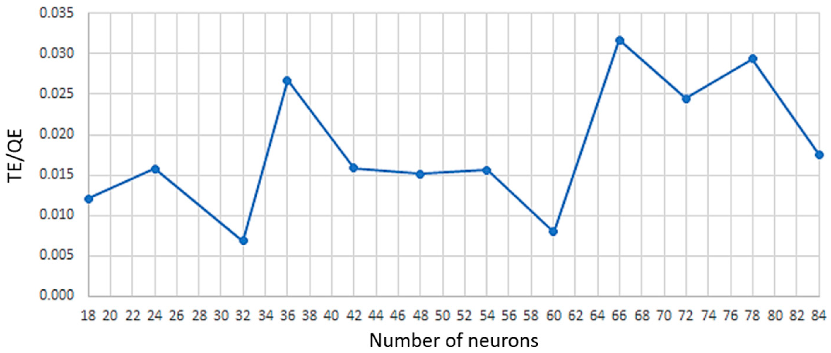
2.2.3. Self-Organizing Maps (SOMs)

SOMs are artificial neural networks characterized by unsupervised training [7]. In these maps, it is possible to project high-dimensional, complex data onto a two dimensional, regularly organized array of discrete locations (neurons) defined by the degree of similarity [6,12]. SOMs are also suitable for clustering the data using clustering methods like k-means and Ward [6,9]. Thus, SOMs achieve two objectives at once: reduce the dimensionality of a problem and display similarities between the data. The construction of any SOM leads to obtaining a prototypical object called codebook vector that is associated to every neuron present in the map [23] and that is assigned to each neuron based on its closeness in the original multi-dimensional space. This means that data points that are close in the multi-dimensional space have nodes that are close on the two-dimensional neural map [6]. The codebook vectors are acquired after iterative updates through the training of the map. This procedure involves three steps: (i) competition between nodes; (ii) selection of a winning node defined as the best-matching unit (BMU); and (iii) update of the codebook vector of each node [6,9,12,13,23]. The SOM algorithm can be initialized using different processes, however, for this study the batch-algorithm with a linear initialization was used, in order to run the whole input data at once and accelerate the training phase [6,9,23]. One critical aspect of the elaboration of the SOM is selecting the topology to order the neurons. The most commonly used are rectangular and hexagonal [23]. However, [23] recommends using a hexagonal topology since it allows each neuron to have six equivalent neighbors (unless the neuron is located at the border of the map) and favors both horizontal and vertical directions. Accordingly, the SOM constructed in this study had a hexagonal topology. The other parameter that must be carefully defined is the dimension of the map. Larger maps allow a more detailed analysis but can have a greater number of empty neurons as well, while smaller maps might lose detail but have a greater predicting capability [23].
Since this is of critical importance, different criteria have been proposed to determine the optimal map size: (i) the optimal number of neurons is close to 5 n [26]; (ii) the ratio of the axes should correspond to the ratio of the standard deviations in the data given by the two largest principal components [23,25] as mentioned above; and (iii) the minimum values of the “quantization error” (QE) and “topographic error” (TE) [23]. Since both errors decrease gradually as the map size increases when using the former criterion, the local minimum values of both errors should be considered [10]. It is important to mention that the criteria can lead to maps with a high number of empty neurons, limiting the reliability of the map [26].
For this study, the approach followed by [12] using the change in the QE/TE ratio associated to different maps was used, taking the number of neurons derived from the [26] equation as the maximum number of neurons to be in the grid and about the ratio between first and second dimension from PCA as the ratio of neurons in the two dimensions. The associated QE and TE were calculated for 12 possible map structures ranging from 30 to 72 neurons using the Kohonen [20] and SOMbrero [21,27] packages. As can be seen in Figure 3 when the number of neurons was 32 (4 × 8), the TE/QE ratio achieved its minimum value. Accordingly, a 4 × 8 map was used throughout this study.
After defining both map size and topology, SOM training can take place. This process will continue until it reaches a predetermined small number, or after a certain number of processing cycles, using many iterations of the learning process to ordinate the codebook vectors [6,13,23]. These vectors have the same dimensions of the original data (i.e., seven) and are commonly visualized as heatmaps that display every dimension in a single 2D grid. An example of the maps obtained using this dataset after 100 iterations, is shown in Figure 4.
The color gradient in these heatmaps, also known as component planes, represents the degree of similarity between adjacent neurons. In the applied color scheme, low values are depicted in blue tones while high values are of sandy shade color. Accordingly, neurons with low concentrations of a given ion will have cooler colors, while neurons with higher concentrations will have more warmer colors (from yellow to sandy shade tones). Finally, SOMs can also be subjected to hierarchical clustering analysis, in order to contribute to the visualization of patterns hidden in large datasets [6,24]. Clustering allows the definition of subgroups based on the distances between each neuron, taking into account that the closer two neurons are to each other, the more similar their codebook vectors and the original values of the variables associated to them are [13,23]. In this study, the clustering approach used was Ward’s linkage method. The optimal number of clusters was defined after confronting 30 different indices using the Nbclust package [28]. The selection of the most suitable number of clusters is based on the calculation of different indices obtained after varying the number of clusters, distance measures, and clustering methods [28].

3. Results and Discussion

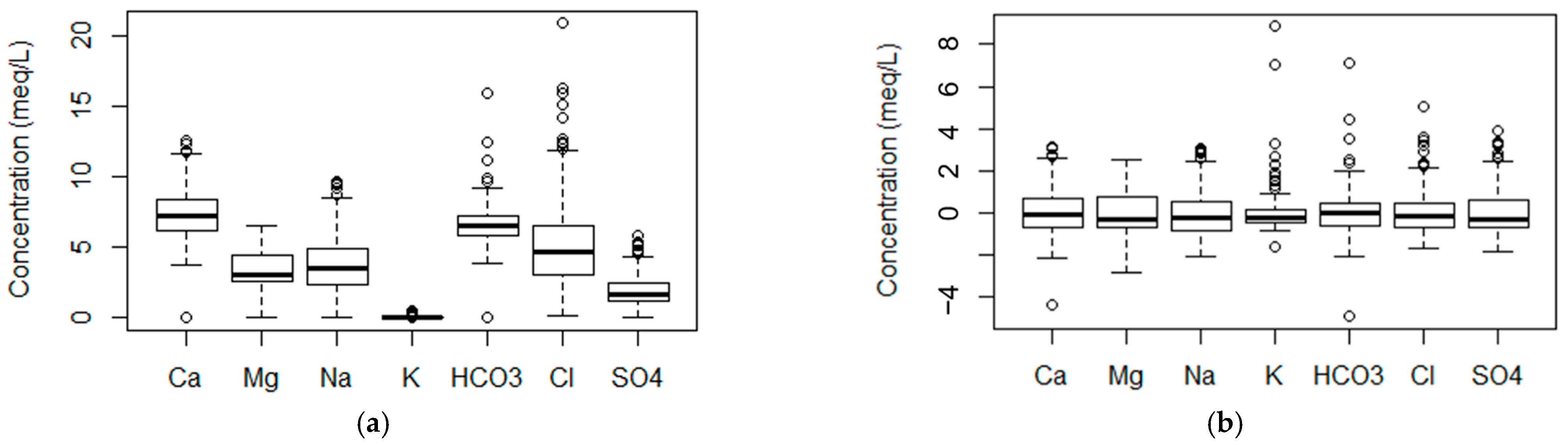
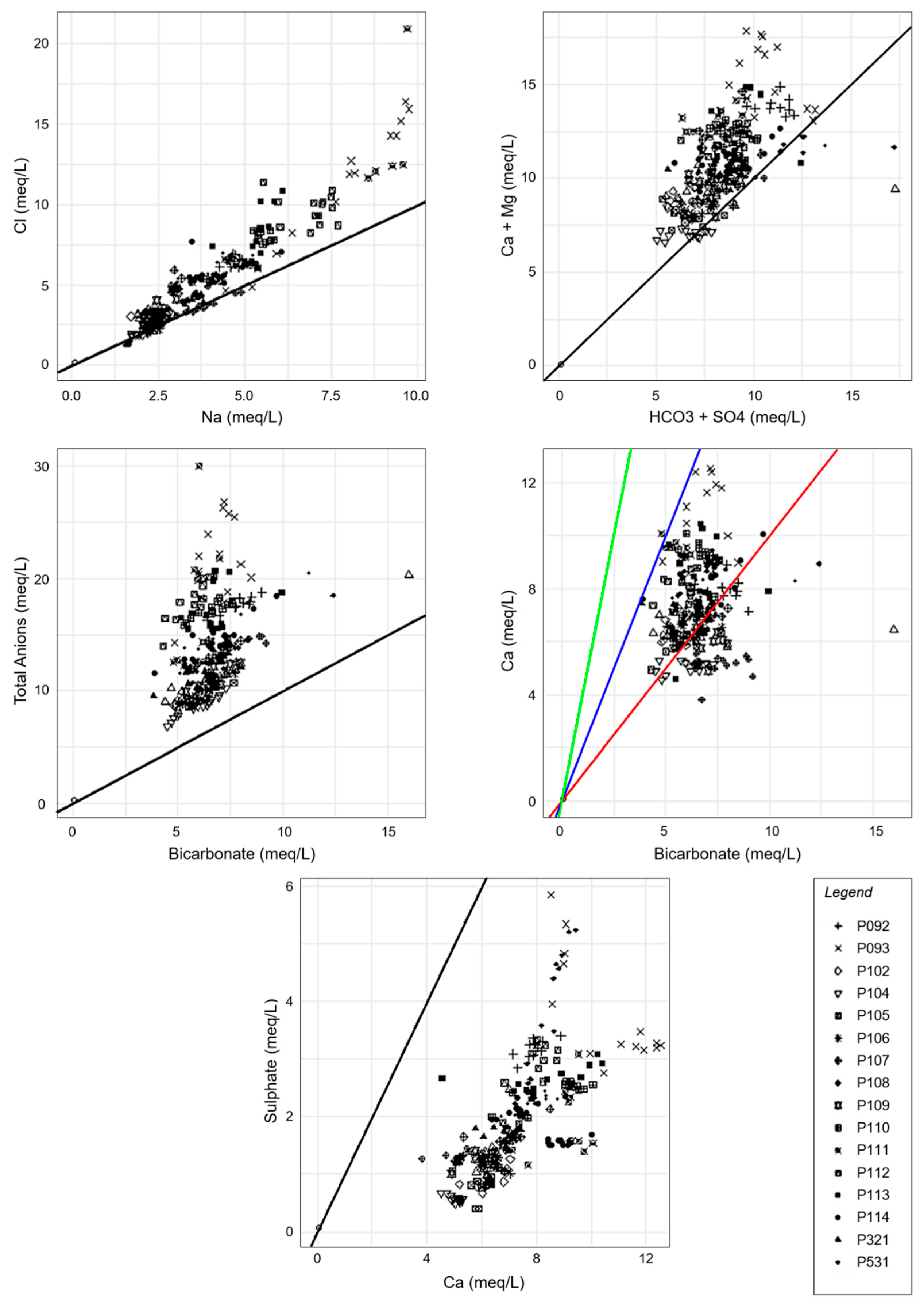
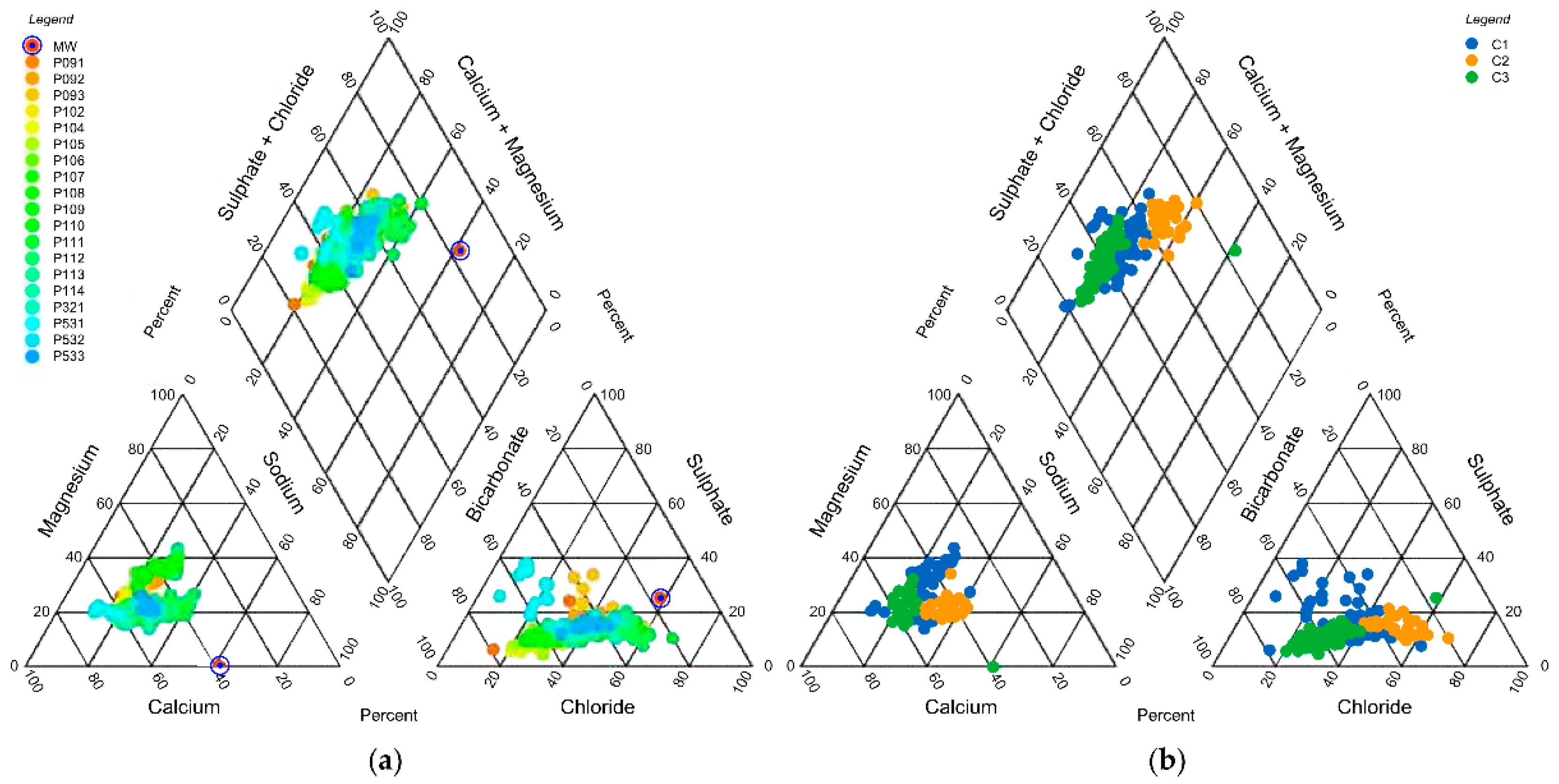
3.1. Hydrogeochemical Characteristics

As shown in Table 1, samples were characterized by high concentrations of Ca2+, HCO3 and Cl as well as very low contents of K+. The fact that for Cl, SO42− and K+ the standard deviation represents almost half of the value for the mean, reflects the high variability of these ions. It also shows that the geochemistry of the study area is not homogeneous. This agrees with the chemical characteristics previously described by [14], and could suggest that there have not been significant changes in the forces that control the chemical characteristics of the groundwaters present between Cecina and San Vincenzo villages in the past 10 years.
As stated by [14], all of the south-west of Tuscany is characterized by the presence of a pre-neogenic substrate (Ligurian, Subligurian and Tuscany Units) discordantly surmounted by clastic-terrigen strata organized in different sedimentary cycles (Upper Tortorian-Pleistocene).
The Tuscany succession was developed during almost 200 MY from the Upper Triassic (Limestones with Rhatavicula contorta) to the Upper Oligocene (boulders) and is characterized by the presence above the platform carbonates from the Lower Lias (solid limestones) of a not very thick basin succession that was carbonate at first, and evolved to a marly-clayey (i.e., Marls with Posidonia) siliceous rocks from the Dogger to the Eocene. This succession emerges quite well along the coast, in Livorno province and in the higher part of the Cecina valley. This geological setting could explain the dominance of both Ca2+ and HCO3 ions in these waters, since the available carbonates might have been dissolved and added to the groundwater system. Further proof of this comes when different ionic relationships are plotted (Figure 5), since according to [29] during rock weathering Ca2+, Mg2+, HCO3 among other ions are added to the groundwater.
From the Na+ vs. Cl plot it can be seen there are two different processes taking place. Most of the samples fall into or are very near the 1:1 ratio. This could be a consequence of halite dissolution or sodium chloride entering the system via rainfall infiltration or sea water intrusion. However, considering the geological setting of the study area, the dissolution of halite is unlikely and other sources of both ions need to be considered. According to [30] sea water can be regarded as the main source of Cl whereas rainwater tends to have low concentrations of this ion. Thus, the influence of saline intrusions into the wells near the coast or affected by an extreme lowering of the piezometric level, is considered as a more plausible explanation for this trend.
The points that show a shift from the 1:1 ratio, also have a greater Na+ concentration. According to [29] this could be a consequence of the occurrence of “natural softening” of the waters. That is, the removal of Na+ ions that are saturating the alluvial sediments in exchange for the Ca2+ ions present in the groundwater due to mineral dissolution. This process takes place when low salinity Ca2+-HCO3 waters flush high salinity waters from an aquifer, since Na-X and Ca-X2 are exchangeable cations [31], with Ca2+ favored in the sorption processes.
However, this process is reversible and it is also possible that Na+ ions, if high concentrations may saturate the alluvial sediments as a consequence of the interaction between the saline intrusion and the lithology with release of Ca2+. The “natural softening” process can also involve Mg2+ ions, resulting in a lowering of its concentrations in the groundwaters and the consequent increase of the amount of Na+ released [14,31]. Natural softening as an explanation for the concentrations observed is also supported by the analysis of the Ca2+ + Mg2+ vs. HCO3 + SO42−, the HCO3 vs. the sum of total anions and the Ca2+ vs. HCO3 plot, all shown in Figure 5. The fact than in the Ca2+ + Mg2+ vs. HCO3 + SO42− plot the majority of the data does not deviate from the 1:1 line, can also be considered as evidence that the Ca2+ and Mg2+ chemistry is largely explained by the weathering process of both calcite and gypsum like minerals [10]. Furthermore, the deviation from the 1:1 ratio in the Ca2+ vs. SO42− plot indicates that this anion is not as influential to the Ca2+ chemistry as other ions present in the groundwaters. This result also agrees with the findings reported by [14,32] for this SSWB. Through a classical hydrogeochemical approach [14] is proposed that the main recharge sources for this aquifer are both the infiltration of local precipitation (especially in lowland areas) and runoff infiltration in the nearby hills. An additional evidence of the influence of rainfall and chemical weathering to the composition of the groundwaters studied, is the fact that all the samples fall between the 1:1 and the 1:2 ratio in the Ca2+ vs. HCO3 plot, since groundwater derived from weathering of dolomite and calcite type minerals usually plot between these equivalent ratios [10].

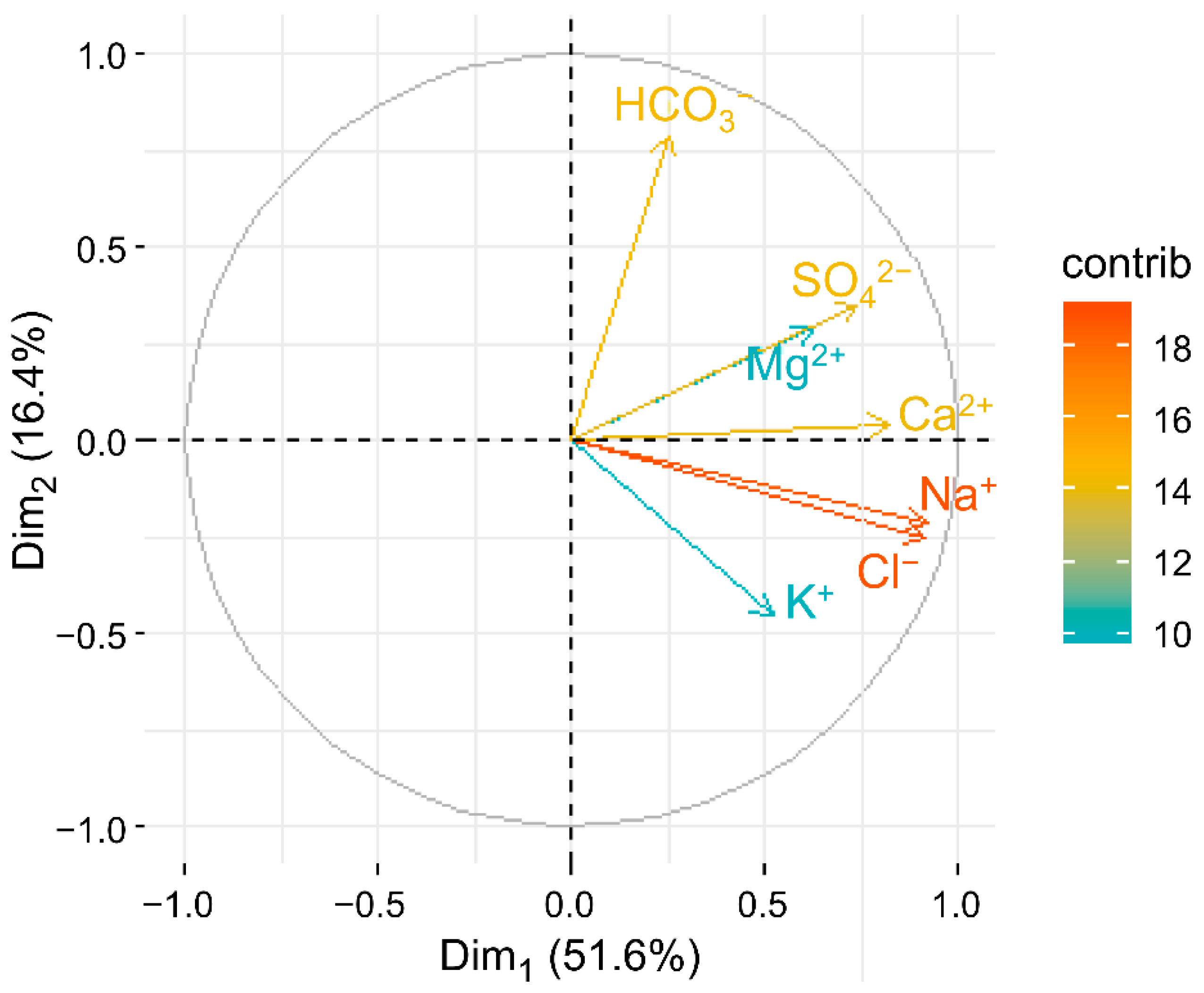
3.2. Principal Component Analysis Applied to Identify the Main Sources of Variability in the Dataset

PCA shows that the first two components explained nearly 70% of the total variance (Figure 6). The first component (Dim 1) has a positive and significant correlation with Na+, Cl, Ca2+, SO42−, Mg2+ and K+, while the second component (Dim 2) positively and strongly relates with HCO3 and SO42−, and in a weak and negative way with Na+, Cl and K+. Both associations could be reflecting the occurrence of two processes, saline intrusion or the weathering processes of the carbonate lithology. Another explanation for the presence of ions such as Na+, Cl and K+ could be the dissolution of evaporitic rocks (gypsum, halite, sylvite). However, according to [14], the presence of halite and sylvite is restricted to two points outside the study area. Thus, the results from the PCA provide further support to the interpretations made in the previous section, of the predominance of rainfall and infiltration as a recharge source for the studied SSWB.
Although K+ and Mg2+ show a relatively small contribution to the overall variance of the dataset, based on their importance to further explain the hydrogeochemical processes taking place in the area, both ions were still used for the rest of the multivariate analyses.

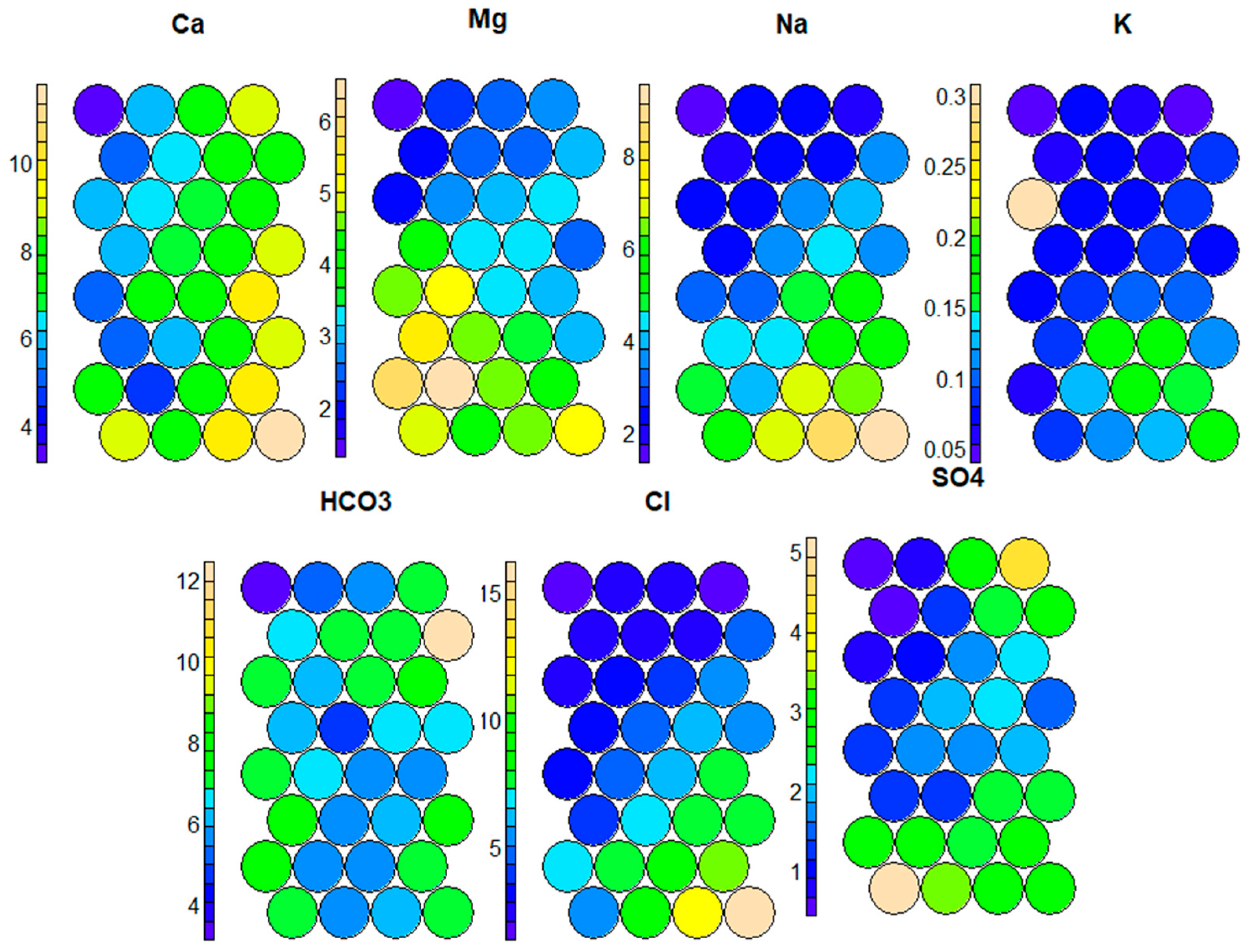
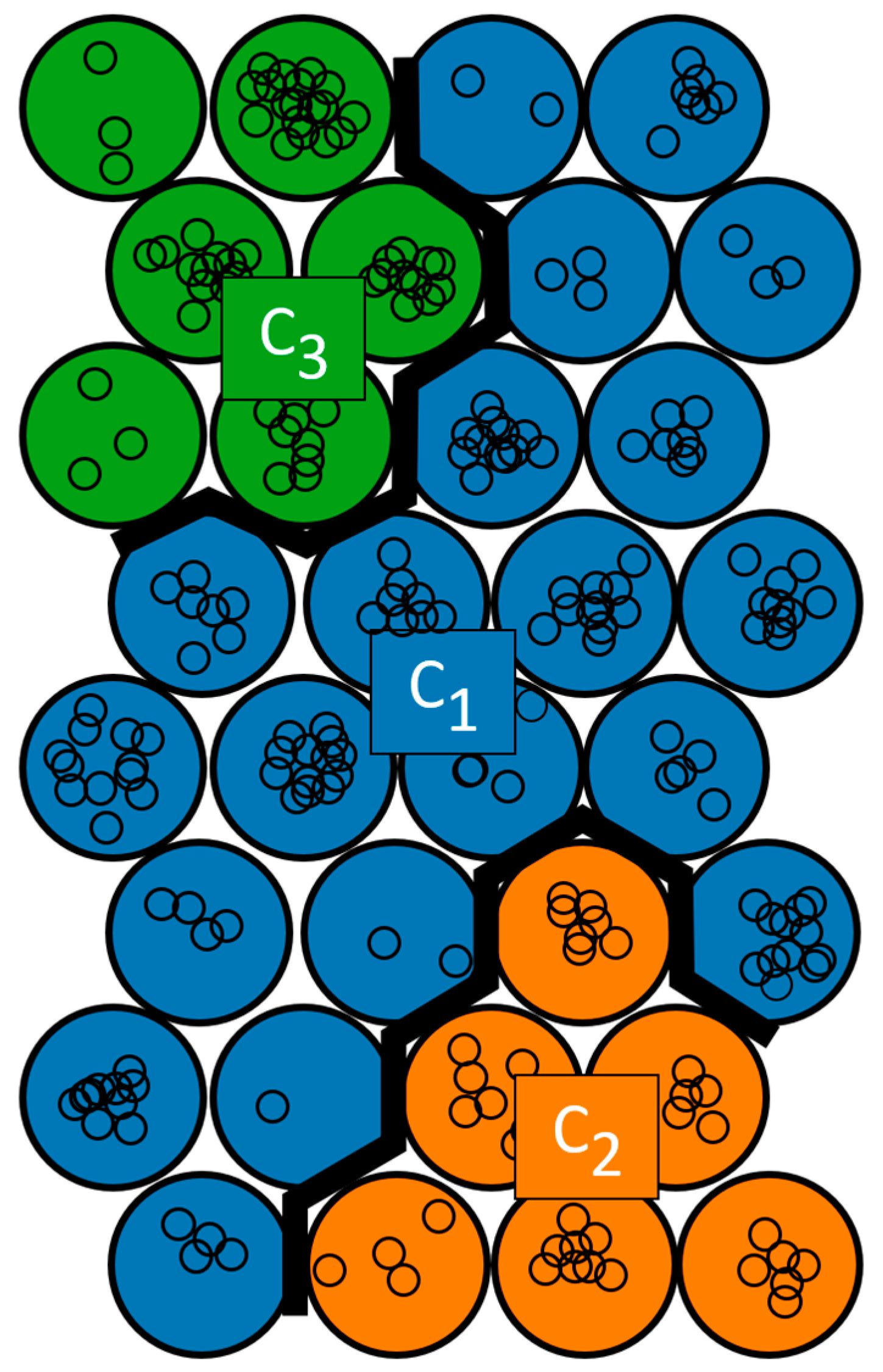
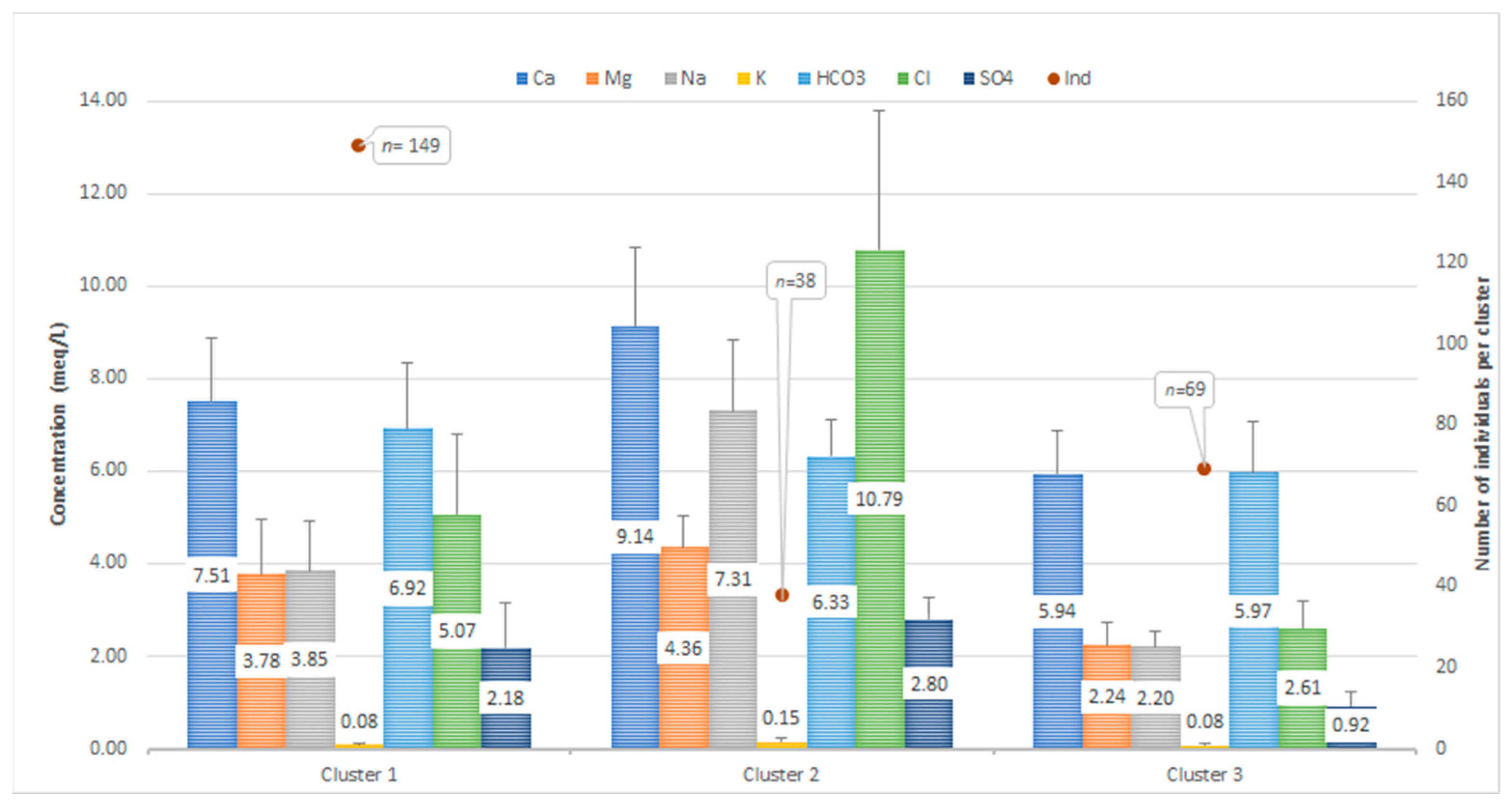
3.3. SOM and Hierarchical Clustering as a Tool for Identification of Groundwater Sources

The use of SOMs coupled to PCA has the additional advantage that the projection of the similarities among variables contains also semi quantitative information about the distribution of the parameters analyzed in the space of the sampling locations; SOM visualization is also able to present simultaneously similarities between positive and negative correlated variables and it also allows the detection of chemical variables that do not associate to a well-defined group [5]. Keeping this in mind, a careful analysis of the similarities between component planes was carried out. There are clear trends in the concentrations of Ca2+, Mg2+, Na+, SO42− and Cl, where higher concentrations are located in the lower area of the neural map (Figure 4). For the same ions, between two and three groups could be easily identified based on visual inspection. A similar differentiation was not possible for the component plane associated with HCO3, possibly reflecting the fact that this ion exerts an important control over the chemistry of the groundwaters throughout the area, a hypothesis previously suggested based on the ionic relationships shown in Figure 6. Following the proposed workflow, the neurons were hierarchically clustered, and the number of clusters was chosen according to the output from the Nbclust code. Since seven tested indices proposed three as the best number of clusters (Table 2), a number that also coincided with the visual differentiation of the component planes initially carried out, this was the number of clusters considered. The clustering obtained is shown in Figure 7.
Wilcoxon-rank and Kruskal–Wallis non-parametric tests were carried out using the dedicated codes in R [17] as an additional validation of the groupings defined after SOM clustering. Both tests confirmed the results obtained with the Nbclust indices and provided further evidence of the fact that these groups had different distributions and could be considered as different populations. The p-values obtained for both tests by testing any possible combination of clusters were lower than 0.05.
In Figure 7, the result of the clustering is shown superimposed to the counts map obtained after constructing the SOM. Each cluster has a specific chemical composition, and reflects the trends previously observed in the component planes. Cluster 1 (149 observations) is characterized by an intermediate chemical composition, having concentrations of all the major ions that fall within the maximum and minimum values for the dataset analyzed. This is by far the largest cluster obtained and could possibly be reflecting the importance of HCO3 in the chemistry of this SSWB’s groundwaters. On the opposite side, there are Clusters 2 and 3, which correspond to waters with more “extreme” chemical compositions. Cluster 2 (38 observations) groups waters that show higher concentrations of all ions, particularly Na+, Cl and SO42− possibly reflecting saline intrusion. Cluster 3 (69 observations) includes waters that are not heavily mineralized and have low concentrations of all major ions. This group also includes the only sample of rainwater available in this study, that was previously characterized by [39].

3.4. Insights from Piper Diagram and SOM Clustering Comparison

The majority of the samples can be found in the upper left side of the Piper diamond, with just a couple of samples plotted on its right side. The large amount of data points together with its similarity in terms of percentage composition would have made it extremely difficult to differentiate between the water types, as can be seen in Figure 8. Thus, the groups obtained after the SOM clustering were plotted in a traditional Piper diagram (Figure 9).
As can be seen from Figure 9B, almost all of our data-points fell within the zone associated with the mixed-water facies. This result was expected if we take into consideration that samples included in this facies do not show a clear predominance of a particular ions, a characteristic attributed to C1, the most populated group obtained. Waters related to C2 showed a more mixed chemistry and a tendency to be more enriched in Cl and F. The majority of the waters associated to C3 plotted on the magnesium-bicarbonate facies presenting low concentrations of Na+ and K+. The only point plotting on the right side of the Piper diamond, is the one associated to the one sample of Tuscany rainwater reported by [39]. This would seem to indicate that there are no similarities between rainwater and those present in the aquifer but the use of the SOM has made it possible to highlight that, even if they do not fall within the same hydrogeochemical facies, these waters have similarities in the codebook vectors which allow them to be inserted in neurons belonging to C3. In the rainwater sample, the Ca2+ and SO42− ions represented about 80% of the total composition, therefore, the influence of the other major ions is not considered important in the definition of the hydrogeochemical facies. Following this multivariate approach, makes it possible to evaluate all the variables simultaneously, and after standardization highlight the presence of similarities on the basis of the trend of the other ions, not considered in the construction of the traditional diagram.

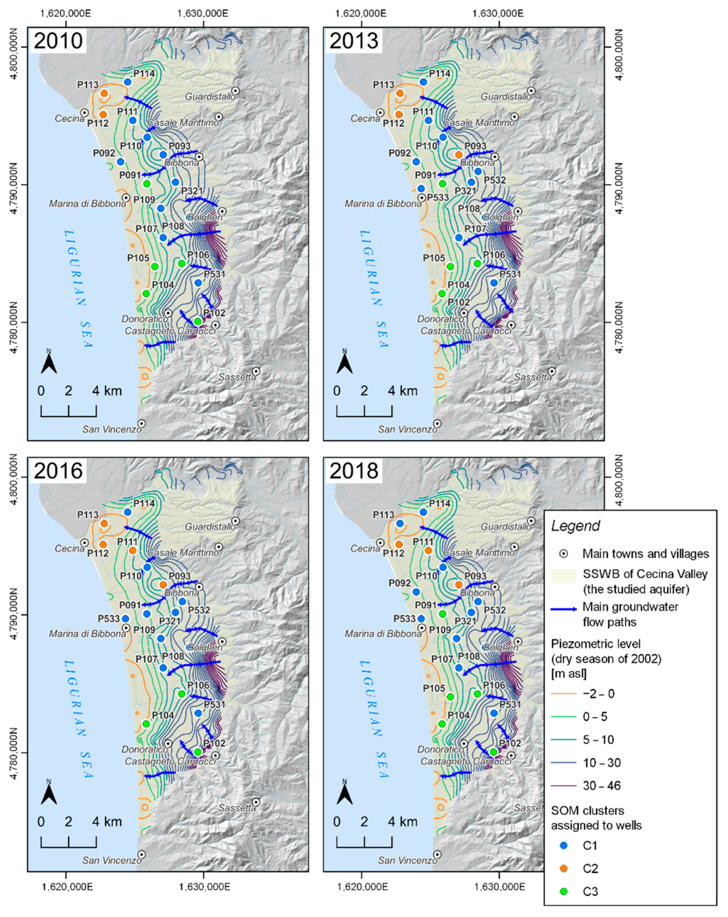
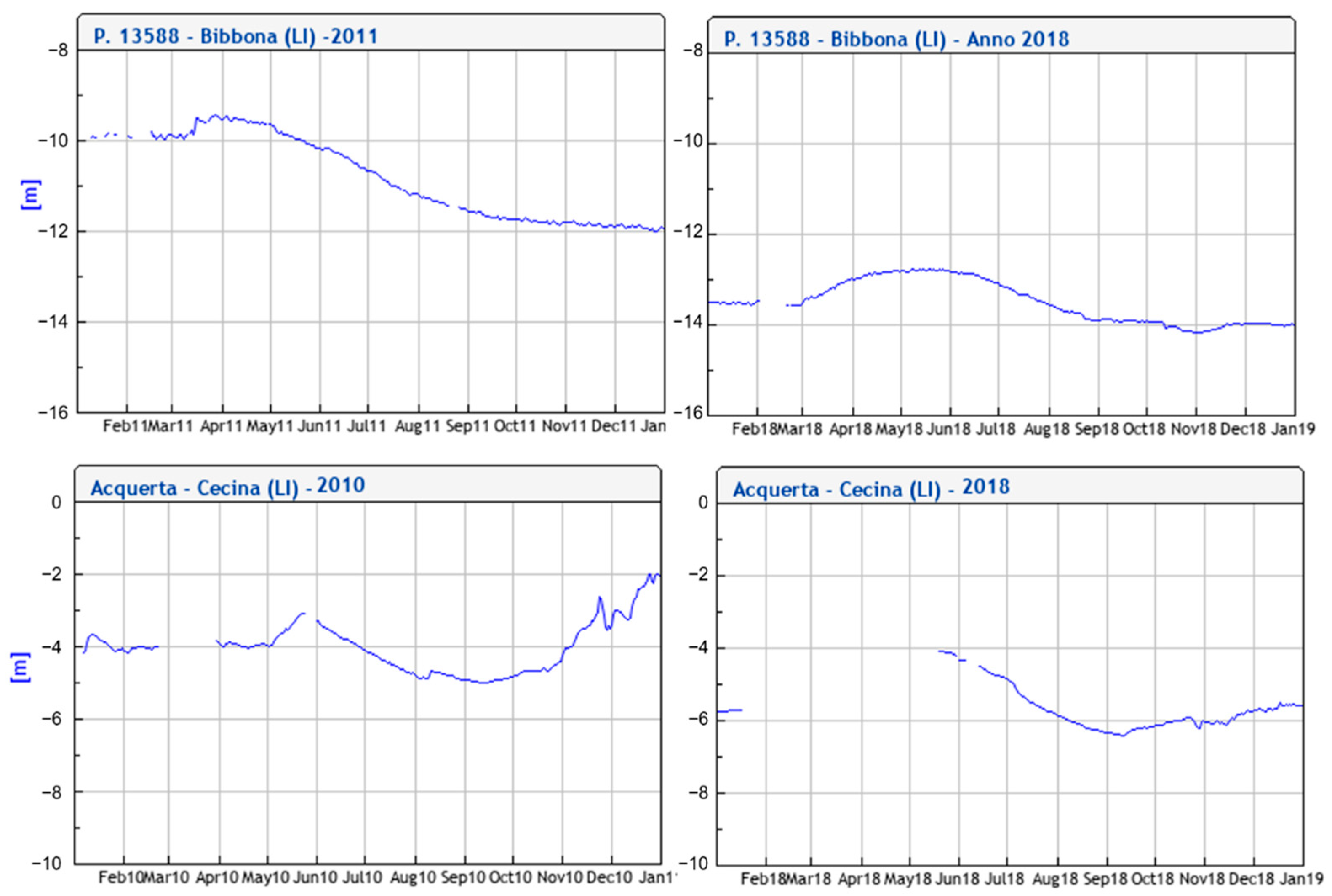
3.5. Seasonal Changes in the Distribution of the SOM Clusters

As previously stated, it is possible to know to which neuron is associated with each well. Since the season and year associated with each sample is also known and specified, it was also possible to detect the occurrence of seasonal changes in water types or within water types through time, after evaluating the presence of the different wells in a specific neuron or cluster. A similar approach was previously undertaken by [9] to evaluate spatio-seasonal hydrogeochemical changes in groundwaters from the Red River Delta in Vietnam. After superimposing the location of the wells with the piezometric level recorded during the dry season of 2002 by [14] (Figure 10) it can be seen that the wells located in the areas where the hydraulic head is below the mean sea level (dashed red lines) were systematically assigned to cluster C2 after 2016. As previously mentioned, C2 was characterized by higher concentrations of Na+, Ca2+ and Cl as well as lower concentrations of HCO3, typical of more saline waters (Table A1, provided in Appendix A). Table A1 summarizes the positioning of all 18 wells within the SOM map during the 6 years analyzed.
The fact that after 2016, there was a shift to more saline waters in two wells very distant to the shore and, apparently not affected by a lowering of the phreatic level (P093 and P111) is of particular concern. Both wells were clustered in C1 from 2010 to 2013, a cluster characterizing samples with a more intermediate groundwater composition and significantly less mineralized than waters included in C2. This situation could be reflecting two phenomena: (i) diminution of the amount of recharge waters received and (ii) increased extraction of water that leads to a lowering of the piezometric level. Both phenomena are not mutually exclusive and could also be taking place simultaneously according to [2,16] for the Tuscany area in a climate change scenario a decrease in the amount and frequency of precipitation should be expected. The shift into a more arid climate would also lead to an increase in the influence of evapotranspiration over the groundwater level [30] increasing the concentrations of the ions in the waters that reach and recharge the groundwater. The visual evaluation of the changes in the phreatic level in areas near these wells (Bibbona for P093 and Cecina for P113) seems to support the above-mentioned hypothesis, since in both areas, from 2011 to 2018 a significant decrease in the phreatic surface is detected. This is particularly true in the Bibbona area, where the levels went from a range between −10 to −12 m to a range between −12 to −14 m (Figure A1, provided in Appendix A).
The other 16 wells analyzed showed changes within the same cluster, moving to adjacent neurons depending on the season. As a general trend, wells moved towards neurons with lower concentrations of all ions (within the same cluster) during the wet season. This is thought to reflect the occurrence of a “dilution effect” during the wetter and rainier season. All wells located at the south of the study area (P102, P104, P105, P106 and P531), were more susceptible to the above-mentioned effect, since there where near a recharge area (i.e., P102 and P531). In addition to this, these wells are all located in the area of Castagneto Carducci, which is characterized by the presence of silty-clayey facies alternated with gravel and conglomeratic ones. Both lithologies are prevalent for at least the first 50 to 70 m and the clays and silts could be acting as a barrier that limits the mixing of the more mineralized waters from the northern area with the ones in the south, especially since according to [14] all the SSWBs present in the coastal area are to be considered as communicating due to the high density of water wells present. Hence, the geological setting combined with the proximity of recharge areas from the mountains, could be taken as probable cause of the fresher character of the waters sampled in these wells.

4. Conclusions

Based on the above-mentioned results (PCA, ionic relations and SOM clustering), it can be confirmed that the recharge source of the aquifers that make up the SSWB of Cecina Valley occurs through the infiltration of fresh waters that equilibrate with the lithologies over which they drain during its movement downstream to the sea. However, the influence of the saline intrusion was also recognized, especially in those areas where due to an overexploitation of the aquifer the piezometric level is lower than the sea level (i.e., P113 in Cecina). The use of a SOM coupled with a hierarchical clustering also allowed the recognition of spatial and temporal patterns that otherwise would have been more difficult to identify using only traditional hydrogeochemical approaches. The results of the clustering of the SOM together with the movements within clusters and among clusters of the sampling wells were likely affected by the changes in hydrodynamic conditions. The multivariate techniques applied, therefore, proved effective in summarizing several years of data and enhancing the interpretation of the hydrogeochemical data. In other study areas, additional parameters, if present, could also be added to the SOM to further refine the statistical analysis and test different conditions, for example the influence of the decreasing aquifer recharge (e.g., from precipitation) and the effect of agricultural activities.

Author Contributions

Conceptualization, A.B. (Alessia Bastianoni), E.G., A.B. (Alessio Barbagli), A.Z., and M.B.; methodology, A.B. (Alessia Bastianoni), A.B. (Alessio Barbagli), and S.B.; software, A.B. (Alessia Bastianoni), S.B.; validation, A.B. (Alessia Bastianoni), A.B. (Alessio Barbagli), and S.B.; formal analysis, S.B.; investigation, A.Z., and M.B.; resources, E.G. and T.C.; data curation, A.B. (Alessia Bastianoni), E.G., A.B. (Alessio Barbagli), A.Z., and M.B.; writing—original draft preparation, A.B. (Alessia Bastianoni), E.G., A.B. (Alessio Barbagli), S.B., A.Z., and M.B.; writing—review and editing, A.B. (Alessia Bastianoni), E.G., and A.B. (Alessio Barbagli); visualization, A.B. (Alessia Bastianoni) and E.G.; supervision, E.G.; project administration, E.G. and T.C.; funding acquisition, E.G. and T.C. All authors have read and agreed to the published version of the manuscript.

Funding

This work was founded by ASA Azienda Servizi Ambientali S.p.A. (the local water utility at Livorno, Italy) and it is part of the larger research and development project named “Superamento delle criticità qualitative e sfruttamento sostenibile della risorsa idrica sotterranea-Toscana costa (overcoming quality problems and sustainable exploitation of groundwater resources-Tuscany coast), 2016–2019”, (ASA purchase order No. OA16001093, of 2 August 2016), performed by GEOexplorer Impresa Sociale S.r.l. (an Italian Small Innovative Enterprise).

Institutional Review Board Statement

Not applicable.

Informed Consent Statement

Informed consent was obtained from all subjects involved in the study.

Data Availability Statement

The dataset used for this study was downloaded from the Tuscany Region Information System: http://sira.arpat.toscana.it/sira/acqua.php (accessed on 17 August 2019).

Conflicts of Interest

The authors declare no conflict of interest.

Appendix A

Table A1. Position of the different wells within the SOM neurons and clusters.
WellYear20102010201120112012201220132013201620162017201720182018
SeasonDryWetDryWetDryWetDryWetDryWetDryWetDryWet
P091Neuron2626302230302618283026222626
ClusterC3C3C3C3C3C3C3C1C1C3C3C3C3C3
P092Neuron55555555 55555
ClusterC1C1C1C1C1C1C1C1 C1C1C1C1C1
P093Neuron11213381434444
ClusterC1C1C2C1C2C2C2C1C2C2C2C2C2C2
P102Neuron2222223030303025222622222622
ClusterC3C3C3C3C3C3C3C3C3C3C3C3C3C3
P104Neuron2525252930293025252525252125
ClusterC3C3C3C3C3C3C3C3C3C3C3C3C3C3
P105Neuron3021253030303026 2630303030
ClusterC3C3C3C3C3C3C3C3 C3C3C3C3C3
P106Neuron26262630303030 262230302126
ClusterC3C3C3C3C3C3C3 C3C3C3C3C3C3
P107Neuron1410141414141414141314141414
ClusterC1C1C1C1C1C1C1C1C1C1C1C1C1C1
P108Neuron99913131313913913131313
ClusterC1C1C1C1C1C1C1C1C1C1C1C1C1C1
P109Neuron131417171717 17171713251713
ClusterC1C1C1C1C1C1 C1C1C1C1C3C1C1
P110Neuron1224121616151612121212121212
ClusterC1C1C1C1C1C1C1C1C1C1C1C1C1C1
P111Neuron2015 1615161643333
ClusterC1C1 C1C1C1C1C2C2C2C2C2
P112Neuron227107277777387
ClusterC2C2C2C1C2C2C2C2C2C2C2C2C2C2
P113Neuron888116111111111211122812
ClusterC2C2C2C2C1C2C2C2C2C1C2C1C1C1
P114Neuron2020202020202020202020241212
ClusterC1C1C1C1C1C1C1C1C1C1C1C1C1C1
P321Neuron2323182322182318232323232323
ClusterC1C1C1C1C3C1C1C1C1C1C1C1C1C1
P531Neuron2727273131323232 3232283232
ClusterC1C1C1C1C1C1C1C1 C1C1C1C1C1
P532Neuron 19181918 2418241919192411
Cluster C1C1C1C1 C1C1C1C1C1C1C1C2
P533Neuron 19182419151918281919191924
Cluster C1C1C1C1C1C1C1C1C1C1C1C1C1
Figure A1. Piezometric levels registered by the Tuscany Region Hydrological Division for the P13588 station in Bibbona (E 1627661, N 4791226) and the “Acquerta” station in Cecina (E 1623732, N 4798039).
Applsci 11 07595 g0a1

References

  1. Cidu, R. Appunti al corso di Idrogeochimica. In Dipartimento di Scienze Chimiche e Geologiche; University of Cagliari: Cagliari, Italy, 2017. [Google Scholar]
  2. D’Angelis, R. Siccità 2016-2017: Il clima cambia e in Italia cresce il rischio idrico. Ecoscienza 2017, 4, 55–91. [Google Scholar]
  3. Piper, A. A graphic procedure in the geochemical interpretation of water-analyses. Trans. Am. Geophys. Union 1944, 25, 914–928. [Google Scholar] [CrossRef]
  4. Durov, S.A. Natural waters and graphic representation of their composition. Dokl. Akad. Nauk SSSR 1948, 59, 87–90. [Google Scholar]
  5. Nisi, B.; Buccianti, A.; Raco, B.; Battaglini, R. Analysis of complex regional databases and their support in the identification of background/baseline compositional facies in groundwater investigation: Developments and application examples. J. Geochem. Explor. 2015, 44, 3–17. [Google Scholar] [CrossRef]
  6. Haselbeck, V.; Kordilla, J.; Krause, F.; Sauter, M. Self-organizing maps for the identification of groundwater salinity sources based on hydrochemical data. J. Hydrogeol. 2019, 576, 610–619. [Google Scholar] [CrossRef]
  7. Astel, A.; Tsakovski, S.; Barbieri, P.; Simeonov, V. Comparison of self-organizing maps classification approach with cluster and principal components analysis for large environmental data sets. Water Res. 2007, 41, 4566–4578. [Google Scholar] [CrossRef]
  8. Choi, B.Y.; Yun, S.T.; Kim, K.H.; Kim, J.W.; Kim, H.M.; Koh, Y.K. Hydrogeochemical interpretation of south Korean groundwater monitoring data using self-organizing maps. J. Geochem. Explor. 2014, 137, 73–84. [Google Scholar] [CrossRef]
  9. Nguyen, T.T.; Kawamura, A.; Tong, T.N.; Nakagawa, N.; Amaguchi, H.; Gilbuena, R. Clustering spatio-seasonal hydrogeochemical data using self-organizing maps for groundwater quality assessment in the red river delta, Vietnam. J. Hydrol. 2015, 522, 661–673. [Google Scholar] [CrossRef]
  10. Ledesma-Ruiz, R.; Pasten-Zapata, E.; Parra, R.; Harter, T.; Mahlknecht, J. Investigation of the geochemical evolution of groundwater under agricultural land: A case study in northeastern Mexico. J. Hydrogeol. 2015, 521, 410–423. [Google Scholar] [CrossRef] [Green Version]
  11. Jankowska, J.; Radzka, E.; Rymuza, K. Principal component analysis and cluster analysis in multivariate assessment of water quality. J. Ecol. Eng. 2017, 18, 92–96. [Google Scholar]
  12. Tsai, W.P.; Huang, S.T.; Cheng, S.P.; Shao, K.T.; Chang, F.J. A data-mining framework for exploring the multi-relation between fish species and water quality through self-organizing map. Sci. Total Environ. 2017, 579, 474–483. [Google Scholar] [CrossRef] [PubMed]
  13. Li, T.; Sun, Y.; Chupeng, G.; Liang, K.; Shengzhong, M.; Lei, H. Using self-organizing map for coastal water quality classification: Towards a better understanding of patterns and processes. Sci. Total Environ. 2018, 628-629, 1446–1459. [Google Scholar] [CrossRef] [PubMed]
  14. Cerrina Feroni, A.; Da Prato, S.; Doveri, M.; Ellero, A.; Lelli, M.; Masetti, G.; Nisi, B.; Raco, B. Caratterizzazione geologica, idrogeologica e idrogeochimica dei corpi idrici sotterranei significativi della regione toscana (CISS): 32CT010 Acquifero costiero tra Fiume Cecina e San Vincenzo, 32CT030 Acquifero costiero tra Fiume Fine e Fiume Cecina, 32CT050 Acquifero del Cecina. In Memorie Della Carta Geologica Italiana; Maretti, P., Ed.; Servizio Geologico d’Itali: Rome, Italy, 2010; pp. 5–80. [Google Scholar]
  15. Angeli, L.; Chiesi, M.; Ferrari, R.; Magno, R. Clima Che Cambia: Gli Impatti Sul Territorio Toscano; Consorzio LaMMA: Florence, Italy, 2012. [Google Scholar]
  16. Zirulia, A.; Brancale, M.; Barbagli, A.; Guastaldi, E.; Colonna, T. Hydrological changes: Are they present at local scales? Rend. Fis. Acc. Lincei 2021, 32, 295–309. [Google Scholar] [CrossRef]
  17. R Core Team. R: A Language and Environment for Statistical Computing; R Foundation for Statistical Computing: Vienna, Austria, 2017. [Google Scholar]
  18. Le, S.; Josse, J.; Husson, F. Facto Mine R: An R Package for Multivariate Analysis. J. Stat. Softw. 2008, 25, 1–18. [Google Scholar] [CrossRef] [Green Version]
  19. Kassambara, A.; Mundt, F. Factoextra R Package: Easy Multivariate Data Analyses and Elegant Visualization. 2017. Available online: http://www.sthda.com/english/wiki/factoextra-r-package-easy-multivariate-data-analyses-and-elegant-visualization (accessed on 17 August 2021).
  20. Wehrens, R.; Buydens, L.M.C. Self-and super-organizing maps in R: The Kohonen package. J. Stat. Softw. 2007, 21, 1–19. [Google Scholar] [CrossRef] [Green Version]
  21. Boelaert, J.; Bendhaiba, L.; Olteanu, M.; Villa-Vialaneix, N. SOMbrero: An R package for numeric and non-numeric self-organizing maps. In Advances in Intelligent Systems and Computing; Villmann, T., Schleif, F.M., Kaden, M., Lange, M., Eds.; Springer: Berlin, Germany, 2014; Volume 295, pp. 5–80. [Google Scholar]
  22. Diekoff, A.L.; Lorenz, D. SMWR Graphs: An R Package for Graphing Hydrologic Data; United States Geological Survey: Reston, VA, USA, 2017.
  23. Wehrens, R. Chemometrics with R: Multivariate Data Analysis in the Natural Sciences and Life Sciences; Springer: Berlin, Germany, 2011. [Google Scholar]
  24. Kohonen, T. Essentials of the self-organizing map. Neural Netw. 2013, 37, 52–65. [Google Scholar] [CrossRef]
  25. Bernardinetti, S.; Bruno, P.P.G. The hydrothermal system of solfatara crater (Campi Flegrei, Italy) inferred from machine learning algorithms. Front. Earth Sci. 2019, 7, 286. [Google Scholar] [CrossRef] [Green Version]
  26. Vesanto, J.; Himberg, J.; Alhoniemi, E.; Parhankangas, J. Self-Organizing Map in Matlab: The SOM toolbox. J. Hydrogeol. 2015, 521, 410–423. [Google Scholar]
  27. Vialaneix, N.; Mariette, J.; Olteanu, M.; Rossi, F.; Bendhaiba, L.; Bolaert, J. SOMbrero: SOM Bound to Realize Euclidean and Relational Outputs. R package version 1.3-1. 2020. [Google Scholar]
  28. Charrad, M.; Ghazzali, N.; Boiteau, V.; Niknafs, A. Nbclust: An R package for determining the relevant number of clusters in a data set. J. Stat. Softw. 2015, 61, 1–36. [Google Scholar] [CrossRef] [Green Version]
  29. Hounslow, A. Water Quality Data: Analysis and Interpretation; Research Gate: Berlin, Germany, 1995. [Google Scholar]
  30. Chiesa, G. Idrogeochimica; Edizioni GEO-GRAPH-Segrate: Milan, Italy, 2005. [Google Scholar]
  31. Appelo, C.A.J. Cation and proton exchange, pH variations, and carbonate reactions in a freshening aquifer. Water Resour. Res. 1994, 30, 2793–2805. [Google Scholar] [CrossRef]
  32. Ufficio Pianificazione del Territorio. Documento Programmatico Per L’avvio Del Procedimento Di Formazione Del Piano Strutturale; Comune di Castagneto Carducci (Provincia di Livorno): Castagneto Carducci, Italy, 2003. [Google Scholar]
  33. Krzanowski, W.J.; Lai, Y.T. A criterion for determining the number of groups in a data set using sum-of-squares clustering. Biometrics 1988, 44, 23–34. [Google Scholar] [CrossRef]
  34. Hartigan, J.A. Clustering Algorithms; John Wiley & Sons, Inc.: Hoboken, NJ, USA, 1975. [Google Scholar]
  35. Milligan, G.W.; Cooper, M.C. An examination of procedures for determining the number of clusters in a data set. Psychometrika 1985, 50, 159–179. [Google Scholar] [CrossRef]
  36. Friedman, H.P.; Rubin, J. On some invariant criteria for grouping data. J. Am. Stat. Assoc. 1967, 62, 1159–1178. [Google Scholar] [CrossRef]
  37. Ratkowsky, D.A.; Lance, G.N. Criterion for determining the number of groups in a classification. Aust. Comput. J. 1978, 10, 115–117. [Google Scholar]
  38. Ball, G.H.; David, J.H. ISODATA, a Novel Method of Data Analysis and Pattern Classification; Stanford Research Inst: Menlo Park, CA, USA, 1965. [Google Scholar]
  39. Brizzio, M.C.; Kotzias, D.; Marchetto, A.; Rembges, D.; Tartari, G.; Mosello, R. The chemistry of atmospheric deposition in Italy in the framework of the national programme for forest ecosystems control (CONECOFOR). J. Limnol. 2002, 61 (Suppl. 1), 77–92. [Google Scholar]
Figure 1. Geological scheme of the study area and the surrounding hills. Legend: 01—Quaternary (post-“Villafranchian”) continental and coastal deposits; 02—Magmatic rocks; 06—Ruscinian and “Villafranchian” continental succession; 07—Pliocene-Pleistocene marine succession; 08—Messinian syn- and post-evaporite succession; 09—Messinian pre-evaporite marine succession; 10—Lower Turolian (Upper Tortonian) fluvio-lacustrine succession; 11—Middle Burdigalian-Lower Tortonian marine deposits (Tyrrhenian Epiligurides Auctt.); 13—Internal Ligurian Domain; 14—External Ligurian Domain; 15—Subligurian Domain; 18—Tuscan Nappe; 21—Tuscan Metamorphic Units; blue line—Tectonic contact; red line—fault; blue dashed line—studied aquifer.
Applsci 11 07595 g001
Figure 2. Boxplot of the concentrations of the major ions in meq/L: (a) distributions before the standardization; (b) distributions after standardization.
Applsci 11 07595 g002
Figure 3. Calculation of the TE/QE ratio for the different SOM sizes evaluated.
Applsci 11 07595 g003
Figure 4. Heatmap of all the parameters used in the training of the SOM. In this figure, blue tones represent low concentrations while high values are of sandy shade color.
Applsci 11 07595 g004
Figure 5. Ionic relationships useful for aquifer matrix characterizations.
Applsci 11 07595 g005
Figure 6. Distribution of the major ions in the first and second component space.
Applsci 11 07595 g006
Figure 7. Clustered SOM. Each color represents a different cluster. The black circles correspond to the individual samples that were included in each neuron. From C1 to C3: result of the three clusters obtained.
Applsci 11 07595 g007
Figure 8. Mean chemical composition of each cluster obtained (columns). Mean concentration is included within each bar. Error bars represent standard deviation. The number of individuals per cluster is represented by the points.
Applsci 11 07595 g008
Figure 9. Piper diagram of the data. The diagram on the left is grouped by well (a). The diagram on the right is grouped according to the SOM clustering results (b). MW represents the meteoric water of the area [39].
Applsci 11 07595 g009
Figure 10. Location of the sampling wells superimposed to the hydraulic head recorded in 2002 according to [14].
Applsci 11 07595 g010
Table 1. Descriptive statistics for the dataset.
UnitCa2+Mg2+Na+K+HCO3ClSO42−
Meanmeq/L7.333.453.920.096.585.251.93
Std. Dev.meq/L1.661.221.890.051.333.101.01
Minimummeq/L0.050.000.080.010.040.140.06
Maximummeq/L12.536.569.740.5416.0120.905.85
Table 2. Indices compared by Nbclust to determine the best number of clusters. KL: maximum value of the index [33]; Hart: maximum difference between hierarchy levels of the index [34]; TrCovW: maximum difference between hierarchy levels of the index [35]; TraceW: maximum value of absolute second; Rubin: minimum value of second differences between levels of the index [36]; Ratk: maximum value of the index [37]; Ball: maximum difference between hierarchy levels of the index [38].
KLHartTrCovWTraceWRubinRatkBall
Number of clusters3333333
Index value2.03.4104.515.10.10.434.7
Number of clusters3333333
Index value2.03.4104.515.10.10.434.7
Publisher’s Note: MDPI stays neutral with regard to jurisdictional claims in published maps and institutional affiliations.

