
Sensor-Level Mosaic of Multistrip KOMPSAT-3 Level 1R Products


1
Department of Civil Engineering, Seoul National University of Science and Technology, Seoul 01718, Korea
2
Department of Civil Engineering, Interdisciplinary Major of Ocean Renewable Energy Engineering, Korea Maritime and Ocean University, Busan 49112, Korea
*
Author to whom correspondence should be addressed.
Appl. Sci. 2021, 11(15), 6796; https://doi.org/10.3390/app11156796
Submission received: 22 June 2021
/
Revised: 22 July 2021
/
Accepted: 22 July 2021
/
Published: 23 July 2021
(This article belongs to the Special Issue Image Simulation in Remote Sensing)
Abstract
:Featured Application
The proposed method can generate a mosaic image at the product level that is corrected only for radiometric and sensor distortions.
Abstract
High-resolution satellite images such as KOMPSAT-3 data provide detailed geospatial information over interest areas that are evenly located in an inaccessible area. The high-resolution satellite cameras are designed with a long focal length and a narrow field of view to increase spatial resolution. Thus, images show relatively narrow swath widths (10–15 km) compared to dozens or hundreds of kilometers in mid-/low-resolution satellite data. Therefore, users often face obstacles to orthorectify and mosaic a bundle of delivered images to create a complete image map. With a single mosaicked image at the sensor level delivered only with radiometric correction, users can process and manage simplified data more efficiently. Thus, we propose sensor-level mosaicking to generate a seamless image product with geometric accuracy to meet mapping requirements. Among adjacent image data with some overlaps, one image is the reference, whereas the others are projected using the sensor model information with shuttle radar topography mission. In the overlapped area, the geometric discrepancy between the data is modeled in spline along the image line based on image matching with outlier removals. The new sensor model information for the mosaicked image is generated by extending that of the reference image. Three strips of KOMPSAT-3 data were tested for the experiment. The data showed that irregular image discrepancies between the adjacent data were observed along the image line. This indicated that the proposed method successfully identified and removed these discrepancies. Additionally, sensor modeling information of the resulted mosaic could be improved by using the averaging effects of input data.
1. Introduction
High-resolution satellite images provide detailed geospatial information with a high geospatial resolution up to 30~80 cm over the area of interest, even located in inaccessible areas. There are many operating satellites such as Ziyuan-3 (2.1 m), KOMPSAT-2 (1 m), Gaofen-2 (0.8 m), TripleSat (0.8 m), EROS B (0.7 m), KOMPSAT-3 (0.7 m), Pléiades 1A/1B (0.7 m), SuperView 1–4 (0.5 m), GeoEye-1 (0.46 m), WorldView-1/2 (0.46 m) and WorldView 3 (0.31 m), etc. [1]. The satellites operate at low altitudes, such as 500,700 km, to achieve a high geospatial resolution of the data. In addition, the satellite cameras are specially designed by increasing the focal length up to around 10 m using a few aspherical mirrors. For example, WorldView-2, Pleiades-HR, and KOMPSAT-3 have focal lengths of 13.311, 12.905, and 8.562 m, respectively.
As a trade-off for the low altitude and long focal lengths, the high-resolution satellite data show a relatively narrow field of view compared to the mid- or low-resolution satellite data. WorldView-3, Pleiades-HR, and KOMPSAT-3, for example, have swath widths of 13.1, 20, and 16.8 km, respectively. Note that mid-/low-resolution satellite data have dozens or hundreds of kilometers of swath width. These high-resolution satellite cameras frequently use a combination of shorter CCD (Charge-Coupled Device) lines with a slight overlap to increase the swath width [2,3,4,5,6]. As examples, IKONOS, Quickbird, KOMPSAT-3 have three, six, and two overlapping PAN CCD lines, respectively, with shifts in the CCD lines in the scan direction. The merge of each sub-scene from CCD lines is carried out with precise camera calibration information. Each sub-scene is processed considering the sensor alignment, ephemeris effects, and terrain elevations to be merged for a single scene covering a larger swath [2,5].
After the sub-scene merging process, high-resolution satellite data are provided in different processing levels. For example, Maxar provides WorldView data in system-ready, view-ready, and map-ready categories. System-ready imagery allows users to perform custom photogrammetric processes such as digital surface model (DSM) generation and orthorectification using the custom data. View-ready imagery data are products already photogrammetrically processed and designed for users interested in remote sensing applications. Map-ready is a base map that has been orthomosaicked. Level 1R and 1G KOMPSAT-3 data from the Korea Aerospace Research Institute are also available. Level 1R is a product that has been corrected for radiometric and sensor distortions. Level 1G is the product corrected for geometric distortions, including optical distortions and terrain effects, and finally projected to a universal transverse mercator coordinate system.
Many satellite data, including WorldView System-ready and KOMPSAT-3 products, are usually delivered in a single image. This is true when the target area is small enough to be located in an archived image region or a new collection less than the swath width is requested. However, in some cases where the area of interest is large and located crossing over the archived images, users are delivered with a bundle of satellite images. Then, the users have to carry out a photogrammetric process for each data bundle to meet their application purposes.
Typical photogrammetric processes with the bundle of images delivered include orthorectification and mosaics to create a complete image map. The orthorectification requires accurate sensor modeling information such as physical model or rational polynomial coefficients (RPCs) and DSM of the target area. In advance of the orthorectification and mosaic, users should carry out bias compensation of the original sensor model information using ground controls to meet mapping requirements [7]. Then, each image is orthorectified for the DSM and the resulting orthoimages are mosaicked for an image map.
There have been many studies for high-resolution satellite image mosaics in the ground coordinates [8,9,10,11,12]. The proposed algorithms deal with radiometric differences in images caused by seasonal changes [8], image registration and cloud detection with removal [9,10], efficient processing [11], and color balancing [12,13]. Most studies are carried out with photogrammetrically processed orthoimages. However, the cost of these photogrammetric processes should increase with the number of images in the delivered bundle.
With a mosaicked image at the sensor level delivered only with radiometric correction, users should take advantage of more efficient and convenient photogrammetric data processing and management for the simplified data. However, no relevant work on the sensor-level image mosaic was carried out before a photogrammetric process. Firstly, if users are delivered with a single image with single sensor model information instead of multiple data sets, the sensor modeling processing burden should be lifted. This is because users do not have to identify the ground control points on the multiple images. In addition, the tie point extraction process over multiple images is not required for accurate co-registration between the images. Secondly, the orthorectification and mosaic process is simplified because the single image orthorectification is simpler, and mosaic methods, including the seamline generation, are not required.
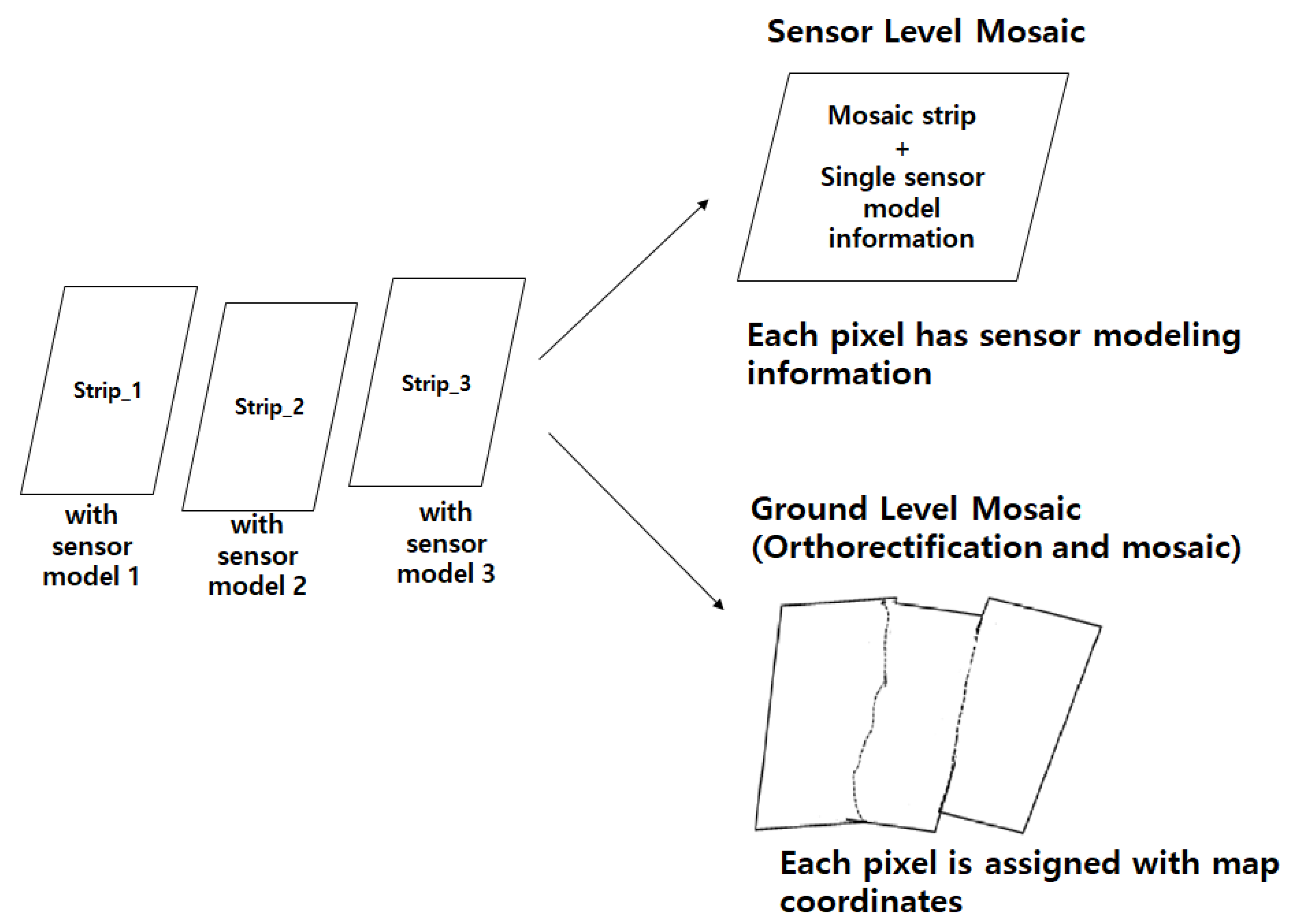
Therefore, we propose a sensor-level mosaic to generate a seamless image product with geometric accuracy to meet mapping requirements. The approach is different than the ground-level mosaic, as depicted in Figure 1. The ground-level mosaic is carried out with the orthorectification of each image strip to the ground, followed by the seamline extraction and mosaic. As a result, each pixel in the mosaicked image is assigned with map coordinates. In contrast, in the sensor-level mosaic, each image is projected into a reference sensor plane to be merged. The resulting image has single sensor modeling information to relate each mosaic image to the ground.
The proposed method begins with setting one image to the reference. Each pixel of the other images is projected to the ground using their sensor model information and SRTM (Shuttle Radar Topography Mission) [14] and then projected into the reference using the reference sensor model information. The problem is that the sensor model information is erroneous such that a large geometric discrepancy occurs due to the satellite’s inaccurate position and attitude information. Therefore, we aimed to model and remove the irregular difference along the image line using the image matching and outlier removal in the overlapped area.
2. Methods
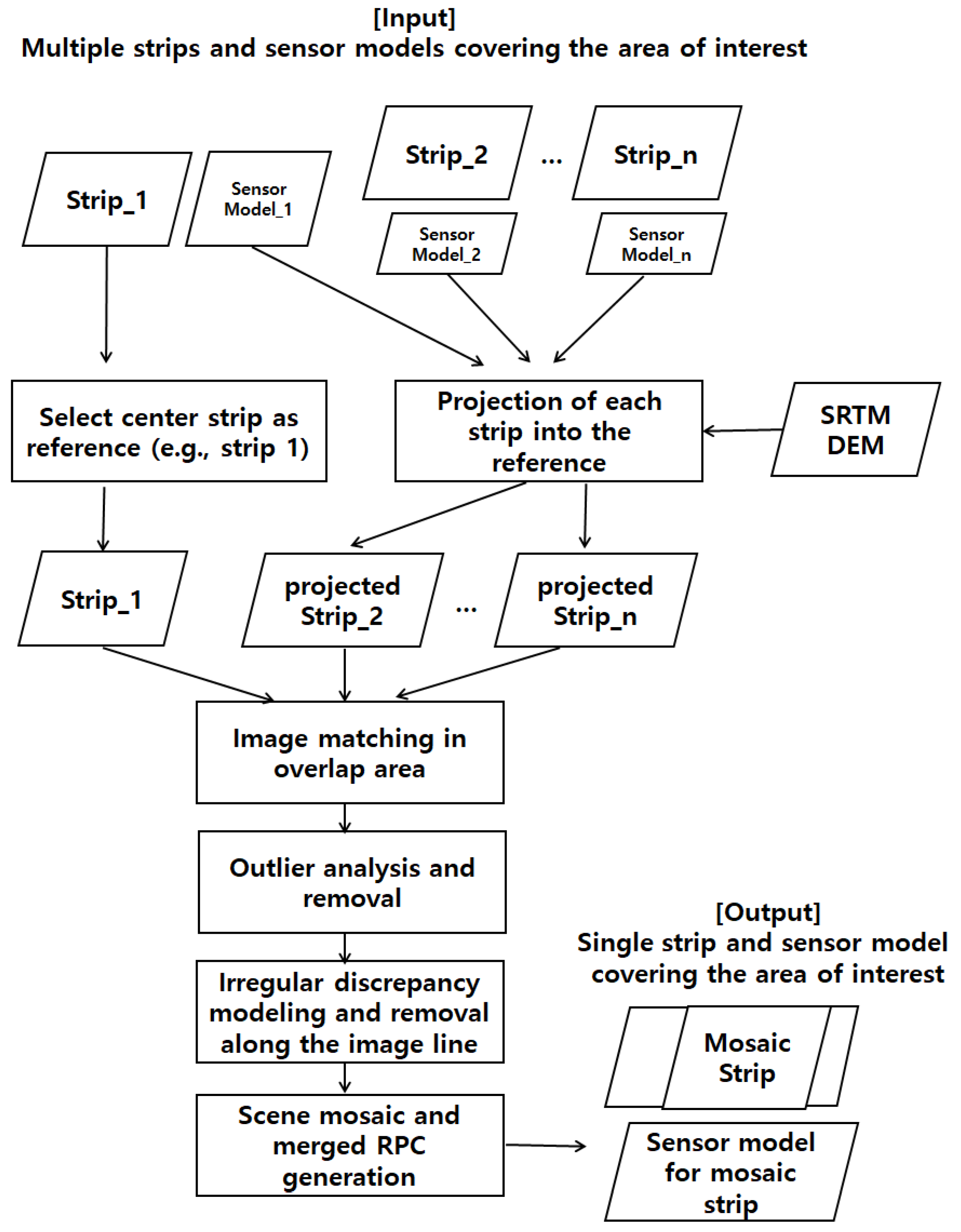
The flowchart of the study is given in Figure 2. Given partially overlapped multiple image strips (n images in the figure) and sensor models covering the area of interest, if one image partially overlapped with other images, it was chosen as the reference image. Each pixel of the other images (collateral images) was first projected to the ground using SRTM DEM and then back-projected onto the reference image space. These projections produce (n − 1) projected images partially overlapped with the reference image. Next, image matching was carried out to extract tie points in the overlap area. A lot of matching outliers should exist because of radiometric and geometric differences, such that it requires detecting and remove them accurately. The discrepancy is expected to show irregular patterns along the image line because of push-broom sensor characteristics. Each line of image has a different position and attitude information. Therefore, we modeled the discrepancy with polynomials after dividing the whole image strip into multiple sub-image regions. Based on the polynomial model, outliers are detected and removed in each sub-image region. This leads to the outlier suppressed tie points set, which enables the irregular discrepancy estimation. The mosaicked image strip can be generated after compensating for the image line discrepancy. Finally, single sensor model information for the mosaic image strip is generated.
2.1. Projection onto the Reference Image
Except for the reference image, the other images, i.e., collateral images, are required to be projected onto the reference image space using the sensor modeling information. This study used RPCs instead of the physical model for compatibility with little difference in accuracy [15].
- 1.
- Ground to image projection:
Ground to image projection is called the forward projection, which equation is expressed as Equation (1). Given 3D ground coordinates , the corresponding image coordinates can be obtained based on the non-linear equation of 78 coefficients (RPCs) [16].
with
where are the geodetic latitude, longitude, and ellipsoidal height. are the image row and column coordinates. and are the normalized image and ground coordinates, respectively. and are the offset and scale factors, respectively for the latitude, longitude, height, column, and row.
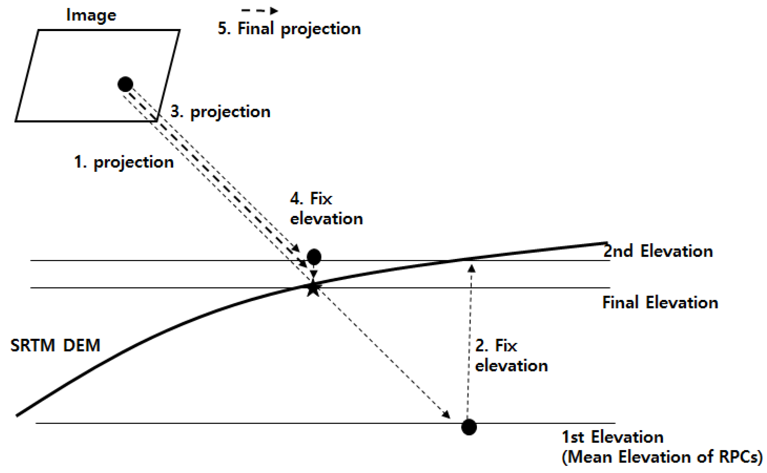
However, the major problem is that the target elevation must be given, and there is no closed solution for the ground elevation computation. Figure 3 depicts the iterative ground elevation search process is depicted. Given an image point, the first image to ground projection is performed to the reference elevation, such as the mean elevation of RPCs. The computed horizontal coordinates are used to look up the ground elevation in SRTM DEM. Next, the second image to ground projection is tried for the estimated ground elevation. This iterative process continues until the no changes in the computed horizontal coordinates.
- 2.
- Image to ground projection:
Image to ground projection is called the backward projection. Given an image coordinates with the ground elevation , the horizontal ground coordinates are computed using Equation (2). The backward projection is a non-linear equation that requires to be linearized as Equation (2). The linearized equation requires the initial horizontal ground coordinates for . The solution is obtained by iteration until it reaches near zero.
where
2.2. Image Matching and Outlier Removal
Image matching in the overlap area is carried out to extract tie points used for discrepancy compensation. This study uses a template matching based on NCC (Normalized Cross-Correlation) as Equation (3). The similarity between reference and projected images is measured using NCC. A matching with NCC larger than 0.5 is typically considered similar, but a higher threshold such as 0.7 is preferred to reduce matching outliers.
where is a patch in the reference image and is a patch within the established search region in the projected image, both are in the size of . are averages of all intensity value in the patches.
These automated image matchings often produce a lot of mismatches that should be detected and removed. RANSAC (Random Sample Consensus) is a popular outlier detection method [17] because it iteratively estimates established modeling parameters from a set of data that includes outliers.
2.3. Piecewise Discrepancy Compensation
High-resolution satellite image strips are acquired using a push-broom sensor that uses a line of detectors arranged perpendicular to the flight direction of the spacecraft. As the spacecraft flies forward, the image is collected one line at a time, with all of the pixels in a line being measured simultaneously.
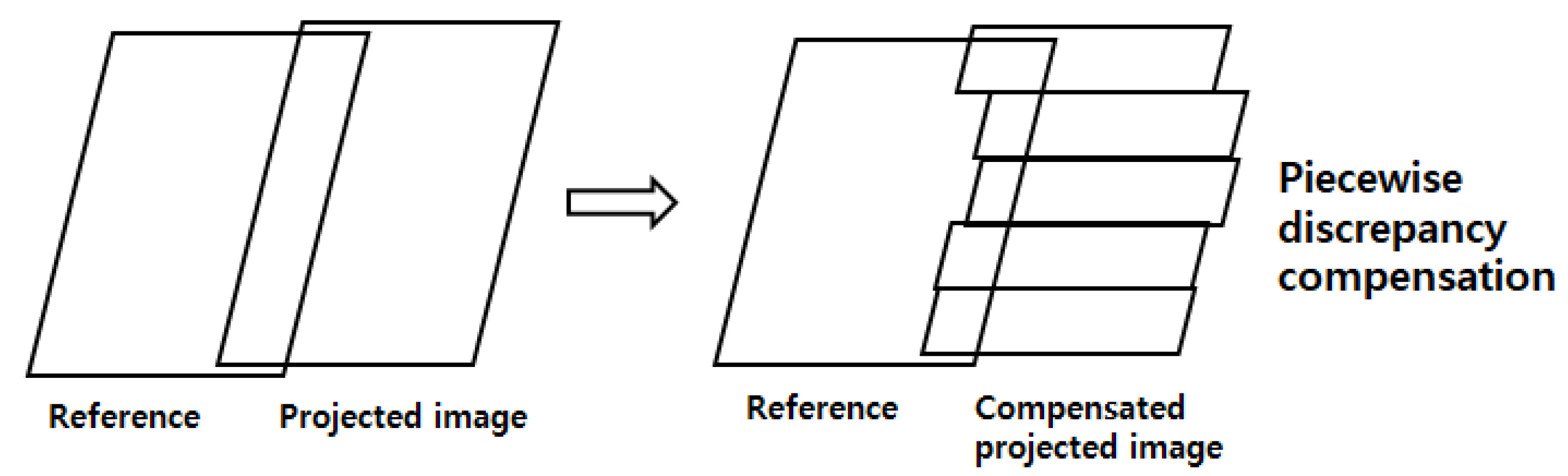
This mechanism should produce an irregular geometric discrepancy between the adjacent strips along the image line. We applied a piecewise discrepancy compensation that models the local difference for some image lines, as depicted in Figure 4. However, it is a possibility of discontinuity between adjacent image pieces. Therefore, we model each local discrepancy with a spline curve.
The sensor model for the mosaic image strip should be generated for photogrammetric processes. Since the mosaic image consists of several image strips of different sensor modeling information, the RPCs for the mosaic can be generated by bias-compensating the RPCs of the reference considering the estimated compensations to the adjacent images [14].
3. Experimental Results
3.1. Data
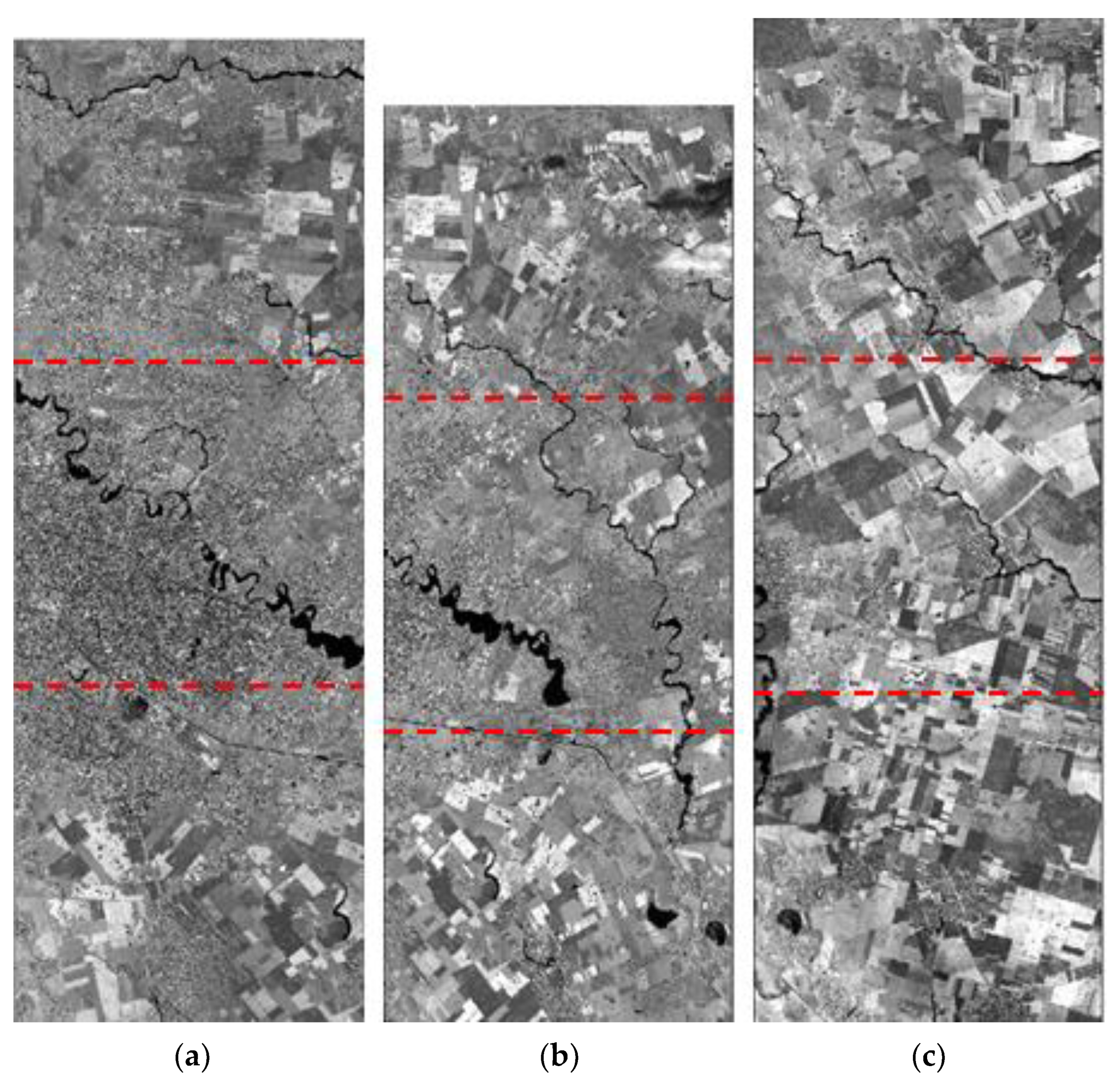
The test data are three image strips of KOMPSAT-3 product level 2R over Romania, as the specifications are listed in Table 1. The acquisition dates are 8 and 24 April and 4 May 2018. The strips have long image line sizes up to 60,000–70,000 pixels with an image swath width of 24,060 pixels. Each image stripe is made up of three image scenes with over 20,000 image lines each. The acquisition geometry includes incidence and azimuth angles. Strips #1 and #3 have similar geometry and a low incidence angle. Small incidence angles of Strips #1 and #3 produce a small GSD (Ground Sample Distance) than Strip #2 with a relatively large incidence angle. Note that the azimuth angle of Strip #2 is in an almost opposite direction from those of the others.
Figure 5 shows the three data strips. Strip #2 is located in the center with partial overlap with the other strips.
3.2. Sensor Modeling of Each Image Strip
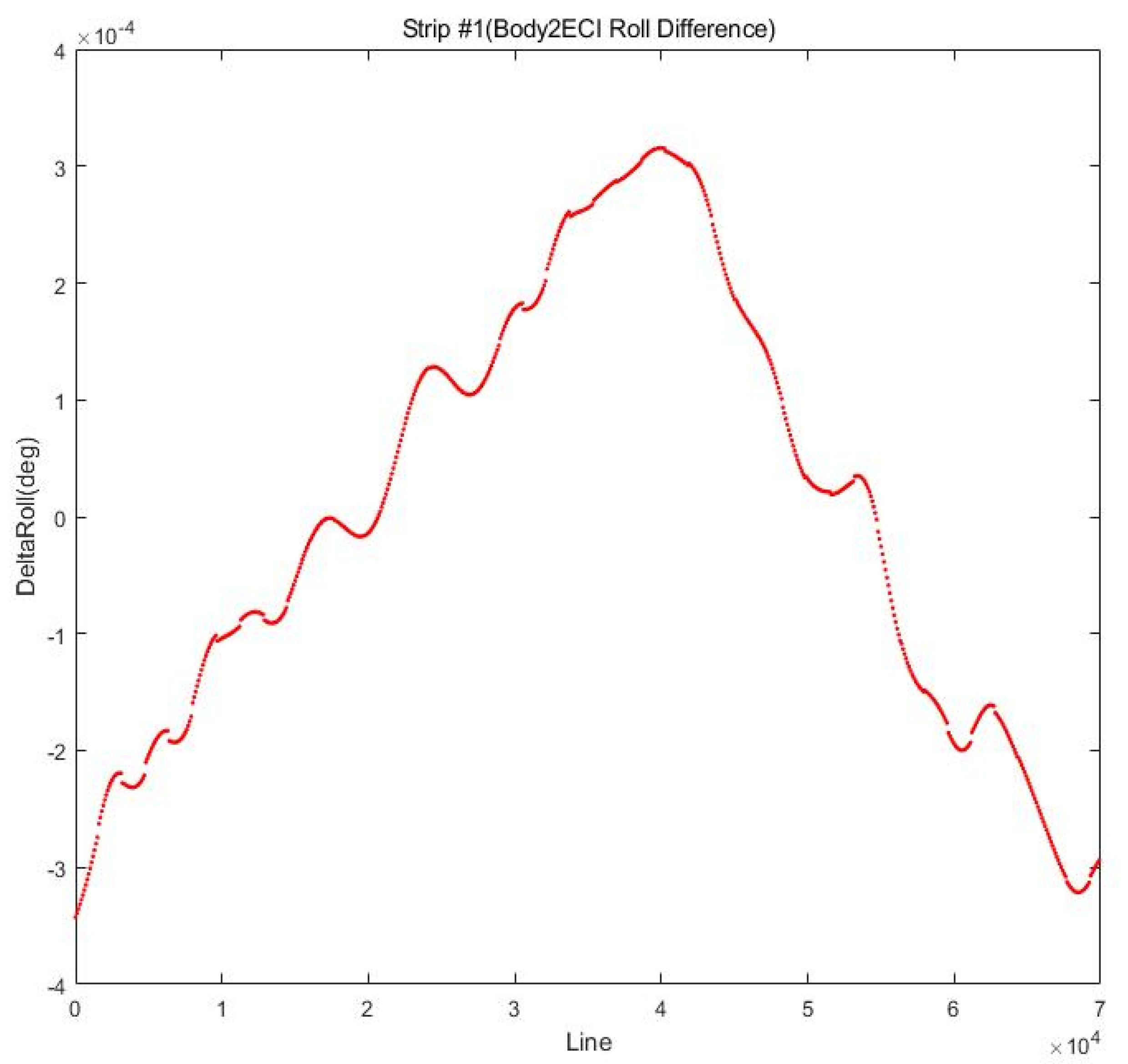
The long strip images were delivered with an ephemeris and attitude data for the physical sensor modeling. However, RPCs are much compatible and easier to use than the physical sensor model, whereas the accuracy is similar. Therefore, we first converted the physical sensor model of each strip into RPCs. The conversion into RPCs is conducted by interpolating satellite attitude information such as roll, pitch, and yaw angles with the first-order equation.
Figure 6 depicts the interpolation residuals for the roll angles of Strip #1, demonstrating that the original roll angle varies locally along the image line. The conversion residuals from the physical model into RPCs are presented in Table 2 for two cases using the original ephemeris and the interpolated ephemeris. Using the interpolated ephemeris shows residuals that are a little better than the other case, which is affected by the local variation in the ephemeris. In Strip #1, the residual in the sample direction improved by more than one pixel.
3.3. Projection of Each Image onto the Reference
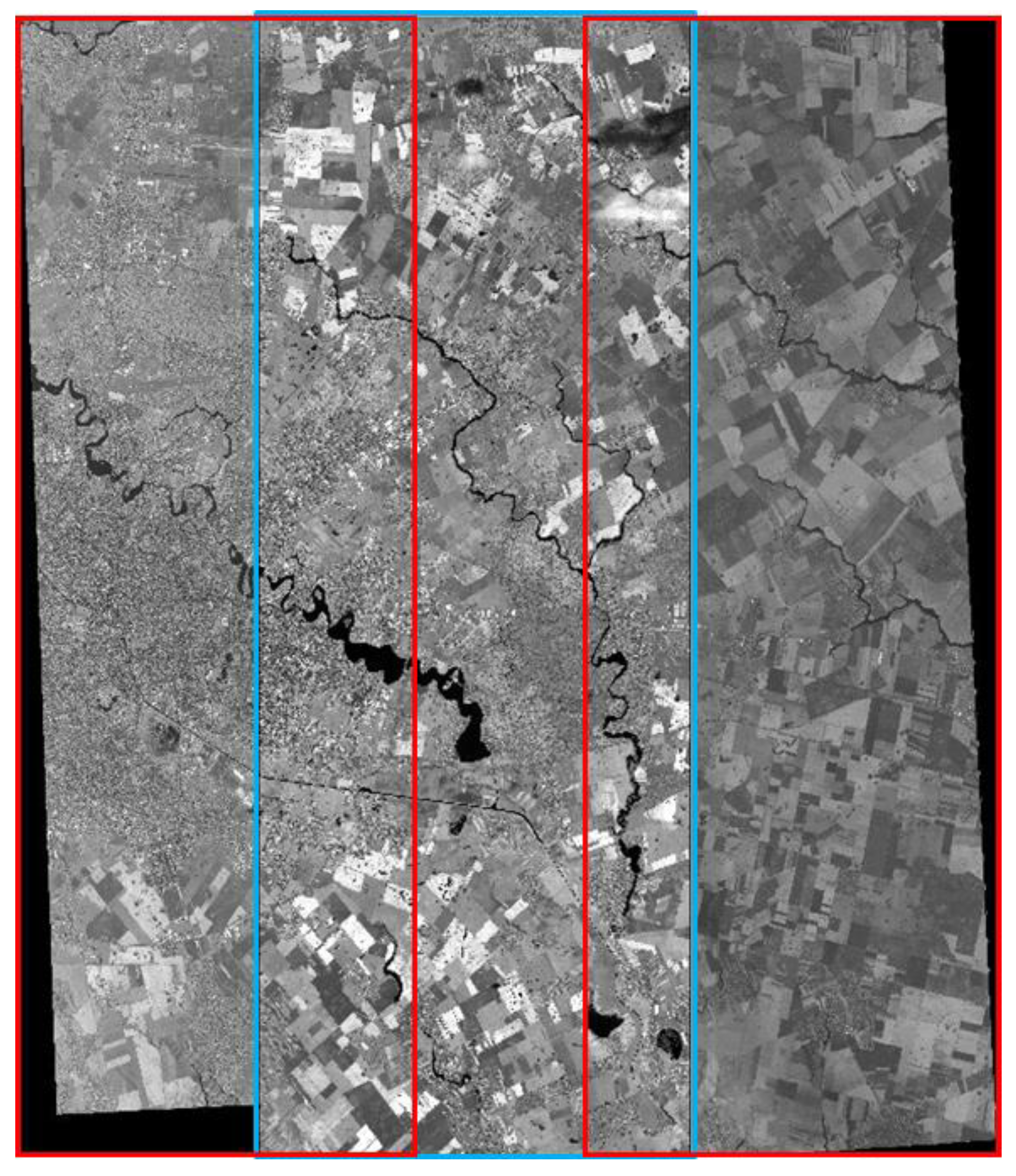
We set the center strip (Strip #2) as the reference. Then, we projected each image onto the reference image space using the generated RPCs with 1 arcsec SRTM DEM. First, the reference image is extended to the sides for the image resampling. A point in the extended reference image space is projected iteratively projected onto SRTM DEM as explained in Figure 3, followed by ground to image projection to look up the corresponding digital number in the adjacent strips. Figure 7 depicts three overlaid stripes side by side.
3.4. Image Matching and Outlier Removal in an Overlap Area
We generated a grid of 50 and 100 pixels along line and sample directions in the overlap area, respectively. Then, we carried out NCC image matching between the reference and the adjacent projected images for the grid points. As matching parameters, we used 77 × 77 pixels for the matching window size, search range 60 pixels. We selected the matching parameters considering the geolocation accuracy of the sensor modeling for KOMPSAT-3, which has 48.5 m (CE90, Circular Error 90% confidence range).
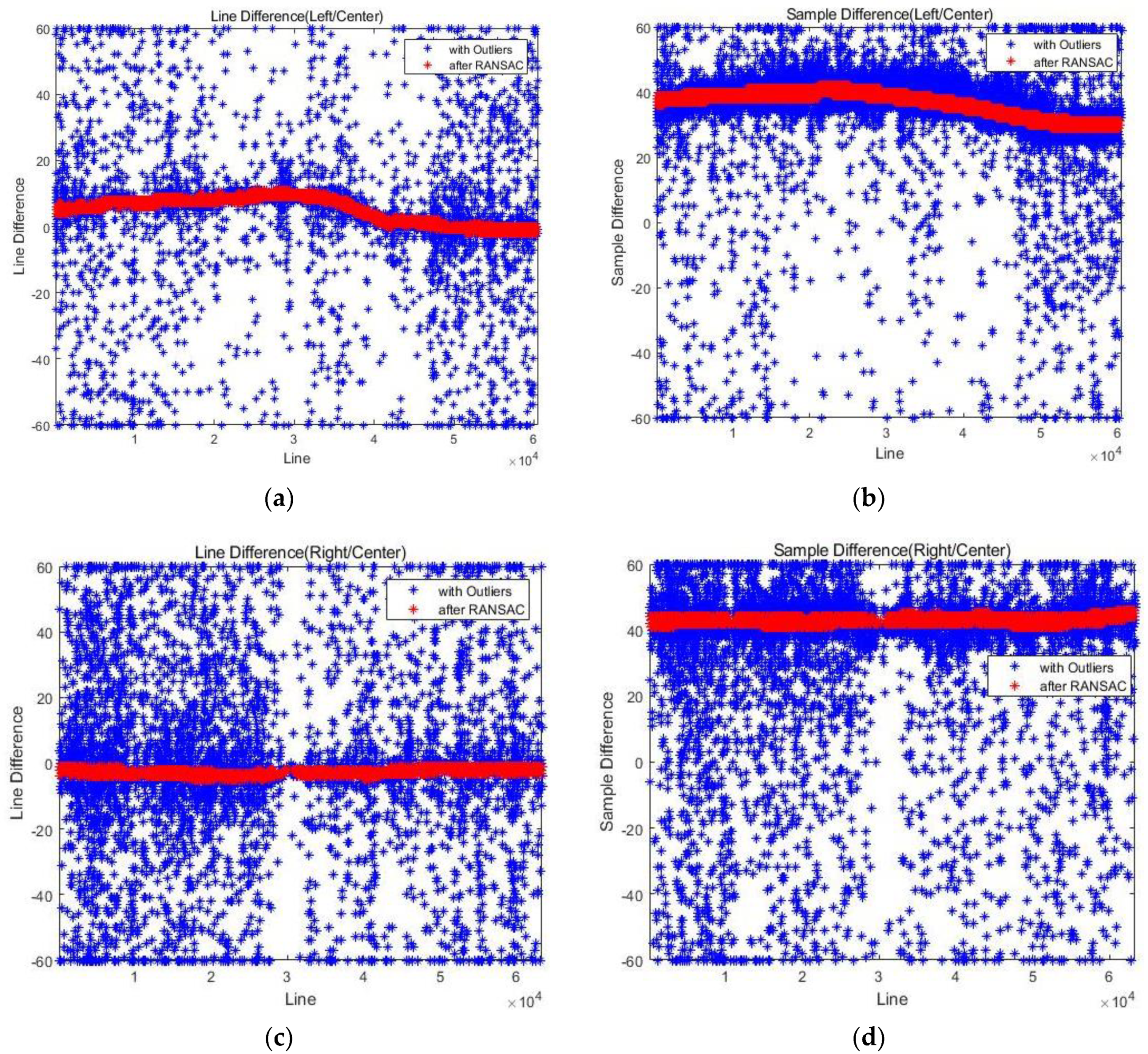
The matching pairs are showing NCC larger than 0.7 were selected as matching candidates in this study. Then, the image coordinates differences were computed between the matching pairs and plotted in Figure 8. Figure 8a,b shows the line and sample coordinates differences between Strips #1 and #2. Figure 8c,d shows the line and sample coordinates differences between Strips #2 and #3. The blue dots show all the coordinates differences for the matching candidates.
We applied the RANSAC algorithm with second polynomial models for each line and sample coordinate differences to suppress the matching outliers. The polynomial model was applied to each scene in an image strip. The red dots show the results after the outlier removal.
3.5. Piecewise Discrepancy Compensation
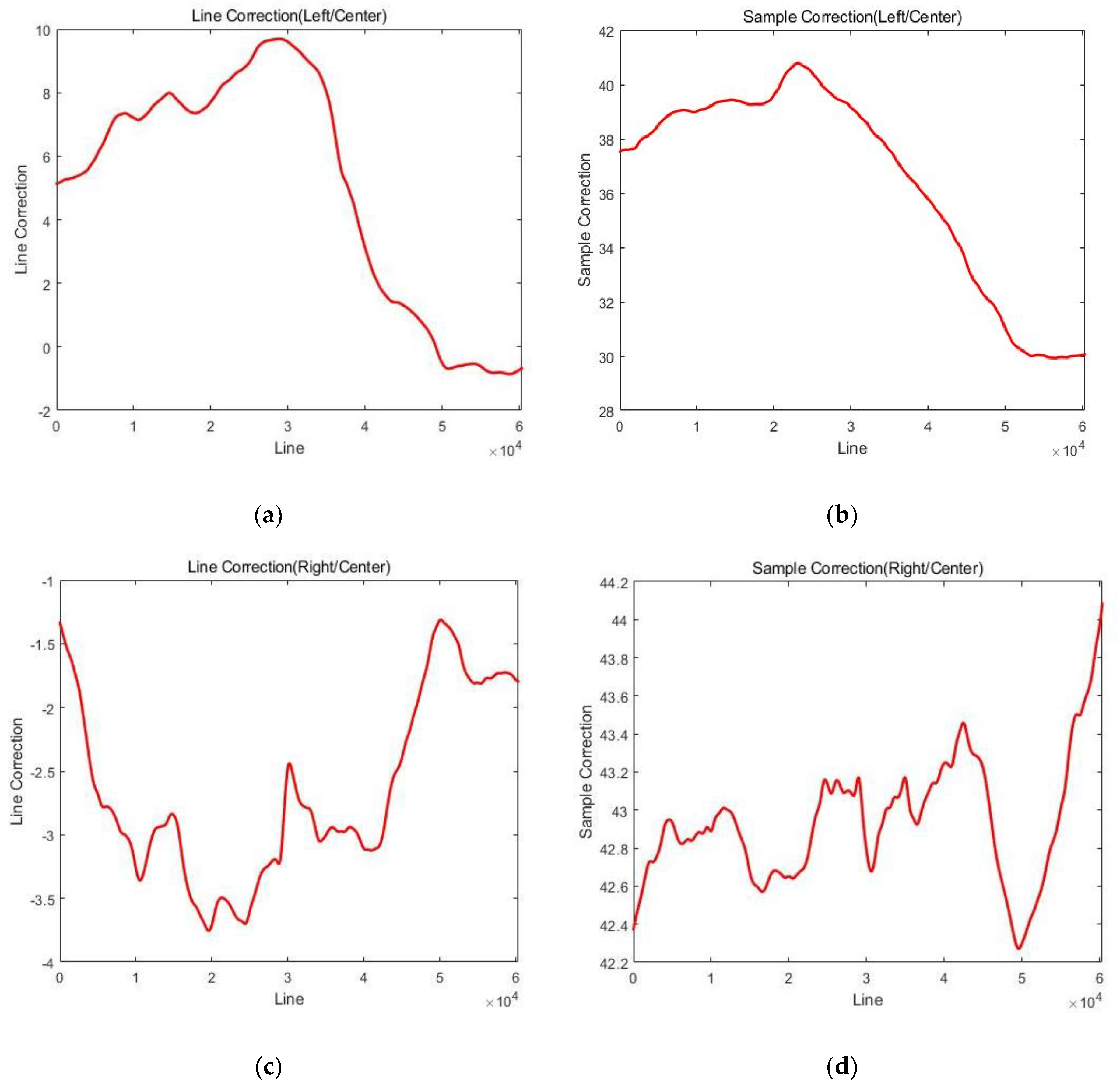
After removing the matching outliers, we can estimate the discrepancy compensation of the projected image by averaging the image coordinates differences between the matching pairs. However, the discrepancy varies for each image line. As shown in Figure 7, averaging single image line discrepancies may produce inaccurate compensation values because there are no redundant matching pairs in an image line. Therefore, we estimated the local discrepancy compensation in the line and sample directions by averaging discrepancies in a block of image lines such as 500 image lines. In addition, we interpolated the averaged differences using a spline curve along the image line to ensure the continuity between compensated image blocks.
Figure 9 shows the estimated local discrepancy for the line and sample directions for every 500 image lines after the spline interpolation. In other words, the red line was derived by averaging the red dots in Figure 8 for every 500 image lines and interpolating them in the spline curve. Figure 9a,b shows the line and sample compensations for Strip #1, and Figure 9c,d are for Strip #3. The rewards for sample coordinates ranging from 30 to 44 pixels are much larger than those for line coordinates.
3.6. Sensor Model Information Generation
As the sensor-level strip mosaic was completed, the sensor modeling information for the single mosaic strip was generated for the photogrammetric process. A 7 × 7 × 7 cubic grid covering the whole mosaic image strips was developed in the ground, and the grid points were projected onto the mosaic strip for the corresponding image coordinates. First, only RPCs of the center strip (Strip #2) were extended to cover the whole mosaic image boundary. Secondly, three RPCs were processed together to generate ground and image coordinate sets for single RPCs generation.
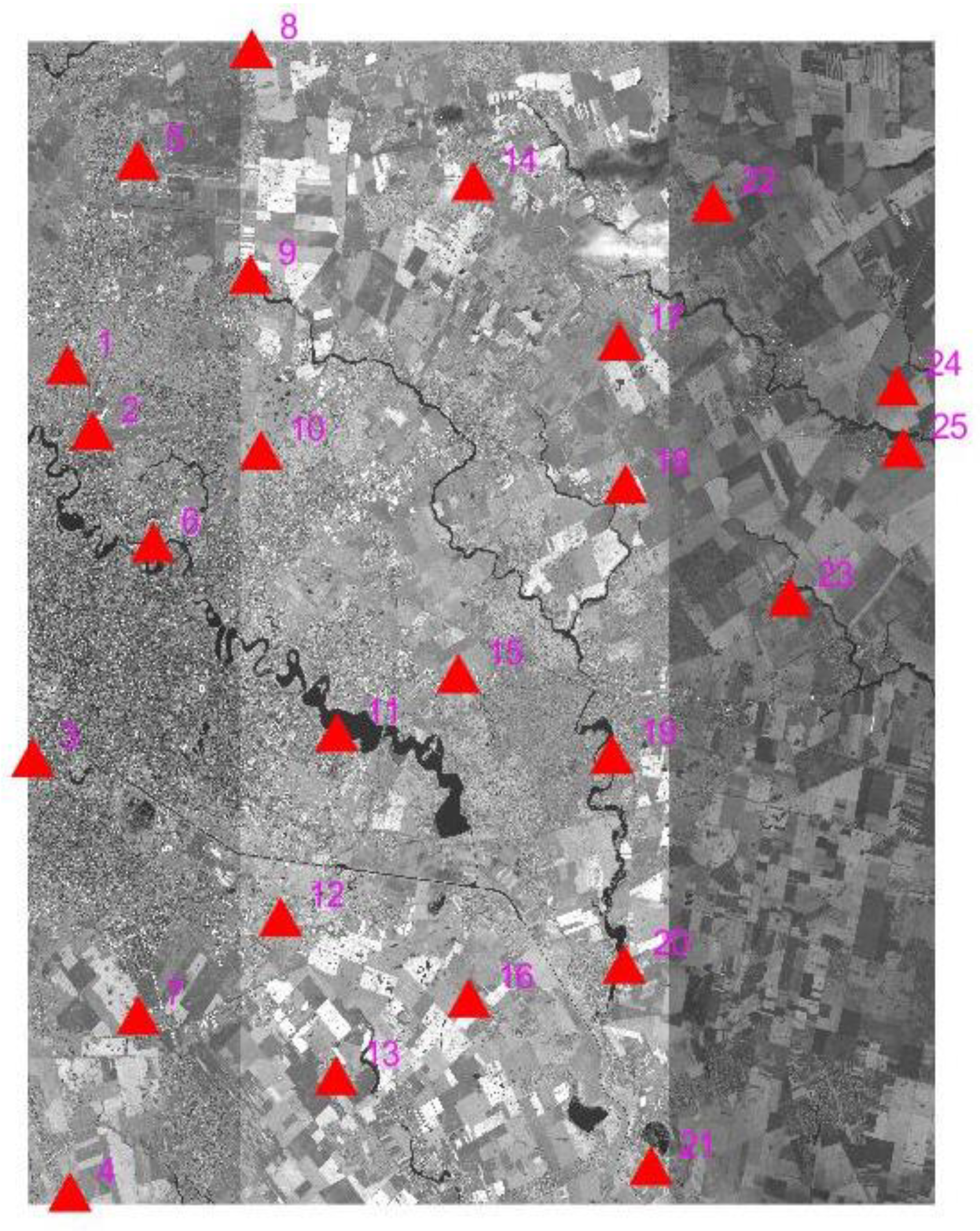
To check the accuracy of the generated RPCs, we collected 25 GCPs over the mosaic strip from Google Earth, as shown in Figure 12. We used Google Earth Pro to extract the horizontal and vertical coordinates. Though the accuracy of Google Earth may differ depending on the areas, a few meters of positional accuracy was reported over near urban areas in Europe [18]. First, using the 25 GCPs as checkpoints, we estimated the accuracy of the aforementioned two RPCs of the center strip and mosaic strip, as shown in Table 3. RPCs of the center strip showed rather low positional accuracy of 4.02 and 40.07 pixels in RMSE for the line and sample directions, respectively. However, the RPCs of the mosaic showed much better results reported as 2.88 and 21.07 pixels in RMSE for line and sample directions. The accuracy improvement ranged from 18% to 47.4%. The geolocation performance of the resulted mosaic RPCs seemed improved due to the averaging effects of all RPCs of input data. The RPCs of the mosaic should be more accurate than the RPCs of each strip if more image strips are used for the mosaic.
Next, the bias compensation of the mosaic RPCs was carried out with the GCPs, and the improved accuracy was presented in Table 4. The bias compensation is a process to improve the input sensor modeling using ground controls. The biases are estimated in image coordinates using the rules and compensated for better accuracy [7]. The errors of the mosaic RPCs were compensated for line and sample directions with constant values estimated from the GCPs. Table 4 shows the RPCs’ accuracy after the compensation process. The compensated RPCs showed adequate accuracies ranging from 1.4 to 3.3 pixels in RMSE compared to the ones shown in Table 3.
4. Discussion
In the study, we used RPCs instead of rigorous sensor modeling. This is for easier and efficient processing as well as compatibility. However, satellite image providers may use the same approach with their physical sensor model. Regarding image matching, the matching window size and search area can be better optimized considering the area of interest and satellite data specification. For example, fewer features would require a larger matching window size, and satellites with precise sensor models would require a smaller search area. In addition, feature-based image matching methods can be used instead [19]. The discrepancy patterns between image strips in line and sample coordinates would be different for satellite data. The data with stable ephemeris would show rather regular discrepancy patterns along the image lines. However, in any case, image compensation should not be carried out for each image line because there are no redundant matching pairs on a single image line. The sensor modeling of the mosaic tends to be more accurate compared to each image strip due to the averaging effects. Therefore, a mosaic of more image strips would produce better positional accuracy [20].
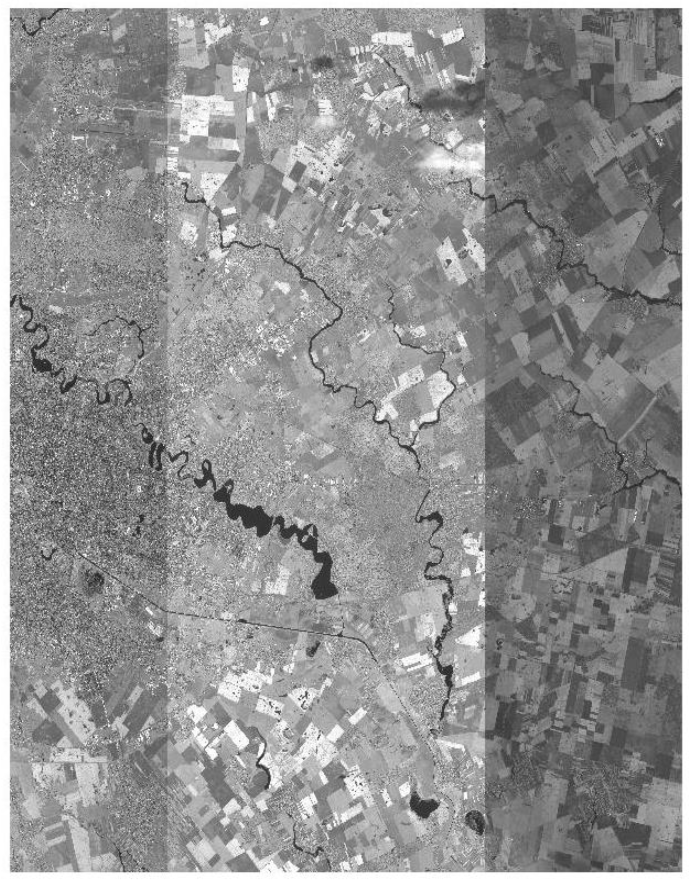
As shown in the resulting mosaic, the three strips’ radiometric differences are observed due to the differences in the acquisition date and angles. The focus of the study is on minimizing the geometric discrepancy and the generation of single sensor model information. Therefore, we have not treated the radiometry in this study, and future research will include the sensor-level radiometric adjustment between the input image strips.
Note that the proposed method is different from the conventional image mosaic carried out with orthorectified images. The proposed sensor-level mosaic is carried out before the photogrammetric processes, including the sensor modeling and orthorectification. Therefore, users can perform their photogrammetric function with the mosaic and the sensor model information.
5. Conclusions
High-resolution satellite images show relatively narrow swath widths such that users often face obstacles to orthorectify and mosaic a bundle of delivered images to create a complete image map. Therefore, the proposed sensor-level mosaicking can generate a seamless image product with improved geometric accuracy. The experimental result with KOMPSAT-3 data showed that the irregular discrepancy between the input images due to the differences in acquisition angles could be minimized for geometrical continuity in the resulted mosaic image. In addition, single sensor modeling information of the mosaic image could be generated for the later photogrammetric processes. The accuracy improvement of the sensor modeling ranged from 18% to 47.4%. Therefore, we believe that the proposed sensor-level mosaic method enables users to take advantage of more efficient and convenient photogrammetric data processing.
Author Contributions
Conceptualization, C.L.; data curation, C.L.; formal analysis, C.L. and J.O.; methodology, C.L. and J.O.; validation, C.L. and J.O.; writing—original draft, J.O.; writing—review and editing, C.L. and J.O. All authors have read and agreed to the published version of the manuscript.
Funding
This study was supported by National Research Foundation of Korea, grant number 2019R1I1A3A01062109.
Institutional Review Board Statement
Not applicable.
Informed Consent Statement
Not applicable.
Data Availability Statement
Not applicable.
Conflicts of Interest
The authors declare no conflict of interest. The funders had no role in the design of the study; in the collection, analyses, or interpretation of data; in the writing of the manuscript, or in the decision to publish the results.
References
- Loghin, A.M.; Otepka-Schremmer, J.; Pfeifer, N. Potential of pléiades and worldview-3 tri-stereo dsms to represent heights of small isolated objects. Sensors 2020, 20, 2695. [Google Scholar] [CrossRef] [PubMed]
- Seo, D.C.; Lee, C.N.; Oh, J.H. Merge of sub-images from two PAN CCD lines of KOMPSAT-3 AEISS. KSCE J. Civ. Eng. 2016, 20, 863–872. [Google Scholar] [CrossRef]
- Pan, H.; Zhang, G.; Tang, X.; Li, D.; Zhu, X.; Zhou, P.; Jiang, Y. Basic products of the ZiYuan-3 satellite and accuracy evaluation. Photogramm. Eng. Remote Sens. 2013, 79, 1131–1145. [Google Scholar] [CrossRef]
- Cheng, Y.; Jin, S.; Wang, M.; Zhu, Y.; Dong, Z. Image mosaicking approach for a double-camera system in the GaoFen2 optical remote sensing satellite based on the big virtual camera. Sensors 2017, 17, 1441. [Google Scholar] [CrossRef] [PubMed] [Green Version]
- Jacobsen, K. Calibration of imaging satellite sensors. In Proceedings of the International Archives of Photogrammetry and Remote Sensing and Spatial Information Sciences, XXXVI-1/W41, Ankara, Turkey, 14–16 February 2006. [Google Scholar]
- Radhadevi, P.V. Pass processing of IRS-1C/1D PAN subscene blocks. ISPRS J. Photogramm. 1999, 54, 289–297. [Google Scholar] [CrossRef]
- Fraser, C.S.; Hanley, H.B. Bias-compensated RPCs for sensor orientation of high-resolution satellite imagery. Photogramm. Eng. Remote Sens. 2005, 71, 909–915. [Google Scholar] [CrossRef]
- Choi, J.; Jung, H.S.; Yun, S.H. An efficient mosaic algorithm considering seasonal variation: Application to KOMPSAT-2 satellite images. Sensors 2015, 15, 5649–5665. [Google Scholar] [CrossRef] [PubMed] [Green Version]
- Zhang, W.; Li, X.; Yu, J. Remote sensing image mosaic technology based on SURF algorithm in agriculture. J. Image Video Proc. 2018, 2018, 85. [Google Scholar] [CrossRef]
- Li, X.; Li, Z.; Feng, R.; Luo, S.; Zhang, C.; Jiang, M.; Shen, H. Generating high-quality and high-resolution seamless satellite imagery for large-scale urban regions. Remote Sens. 2020, 12, 81. [Google Scholar] [CrossRef] [Green Version]
- Chen, H.; He, H.; Xiao, H.; Huang, J. A fast and automatic mosaic method for high-resolution satellite images. In Proceedings of the SPIE 9808, International Conference on Intelligent Earth Observing and Applications, Guilin, China, 9 December 2015. [Google Scholar] [CrossRef]
- Cresson, R.; Saint-Geours, N. Natural color satellite image mosaicking using quadratic programming in decorrelated color space. IEEE J. Sel. Top. Appl. Earth Obs. Remote Sens. 2015, 8, 4151–4162. [Google Scholar] [CrossRef] [Green Version]
- Wegmueller, S.A.; Leach, N.R.; Townsend, P.A. LOESS radiometric correction for contiguous scenes (LORACCS): Improving the consistency of radiometry in high-resolution satellite image mosaics. Int. J. Appl. Earth Obs. Geoinf. 2021, 97, 102290. [Google Scholar] [CrossRef]
- Farr, T.G.; Rosen, P.A.; Caro, E.; Crippen, R.; Duran, R.; Hensley, S.; Kobrick, M.; Paller, M.; Rodriguez, E.; Roth, L.; et al. The shuttle radar topography mission. Rev. Geophys. 2007, 45. [Google Scholar] [CrossRef] [Green Version]
- Dial, G.; Grodecki, J. RPC Replacement Camera Models. In Proceedings of the American Society for Photogrammetry and Remote Sensing 2005 Annual Conference, Baltimore, MD, USA, 7–11 March 2005. [Google Scholar]
- Grodecki, J. IKONOS stereo feature extraction—RPC approach. In Proceedings of the ASPRS 2001, St. Louis, MO, USA, 23–27 April 2001. [Google Scholar]
- Fischler, M.A.; Bolles, R.C. Random sample consensus: A paradigm for model fitting with applications to image analysis and automated cartography. Commun. ACM 1981, 24, 381–395. [Google Scholar] [CrossRef]
- Pulighe, G.; Baiocchi, V.; Lupia, F. Horizontal accuracy assessment of very high resolution Google Earth images in the city of Rome, Italy. Int. J. Digit. Earth. 2016, 9, 342–362. [Google Scholar] [CrossRef]
- Oh, J.; Han, Y. A double epipolar resampling approach to reliable conjugate point extraction for accurate Kompsat-3/3A stereo data processing. Remote Sens. 2020, 12, 2940. [Google Scholar] [CrossRef]
- Rottensteiner, F.; Weser, T.; Lewis, A.; Fraser, C.S. A strip adjustment approach for precise georeferencing of ALOS optical imagery. IEEE Trans. Geosci. Remote Sens. 2009, 47, 4083–4091. [Google Scholar] [CrossRef]
Figure 1.
Sensor-level mosaic vs. ground-level mosaic.

Figure 2.
Flowchart of the proposed method for the sensor-level mosaic.

Figure 3.
Iterative ground elevation search.

Figure 4.
Piecewise discrepancy compensation.

Figure 5.
Test image strip of three scenes: (a) Strip #1, (b) Strip #2, (c) Strip #3.

Figure 6.
Difference between the original and the interpolated roll angles (Strip #1).

Figure 7.
Projected images onto the reference image space.

Figure 8.
Discrepancy between the image coordinates in the matching pair—(a) line difference between Strips #1 and #2; (b) sample difference between Strips #1 and #2; (c) line difference between Strips #2 and #3; (d) sample difference between Strips #2 and #3.
Figure 8.
Discrepancy between the image coordinates in the matching pair—(a) line difference between Strips #1 and #2; (b) sample difference between Strips #1 and #2; (c) line difference between Strips #2 and #3; (d) sample difference between Strips #2 and #3.

Figure 9.
Estimated discrepancy compensation—(a) line compensation for Strip #1; (b) sample compensation for Strip #1; (c) line compensation for Strip #3; (d) compensation for Strip #3.
Figure 9.
Estimated discrepancy compensation—(a) line compensation for Strip #1; (b) sample compensation for Strip #1; (c) line compensation for Strip #3; (d) compensation for Strip #3.

Figure 10.
Final strip mosaic.

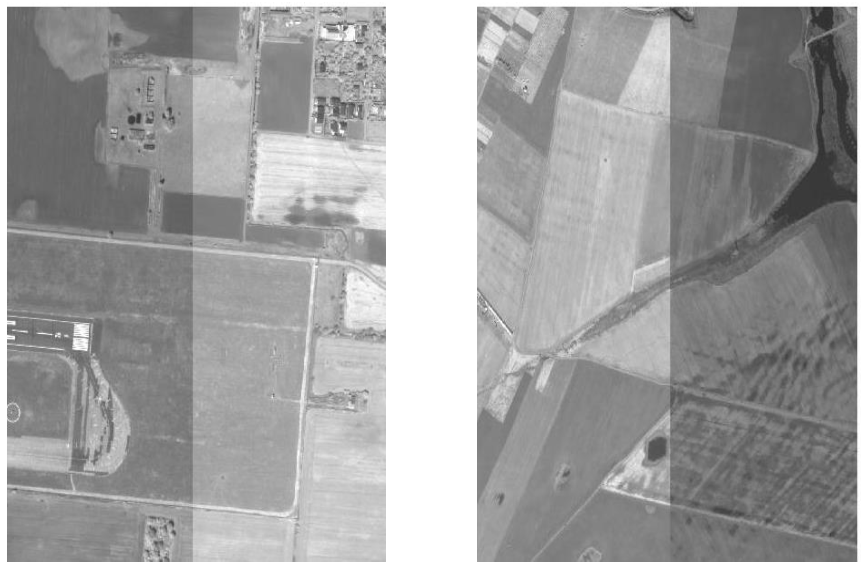
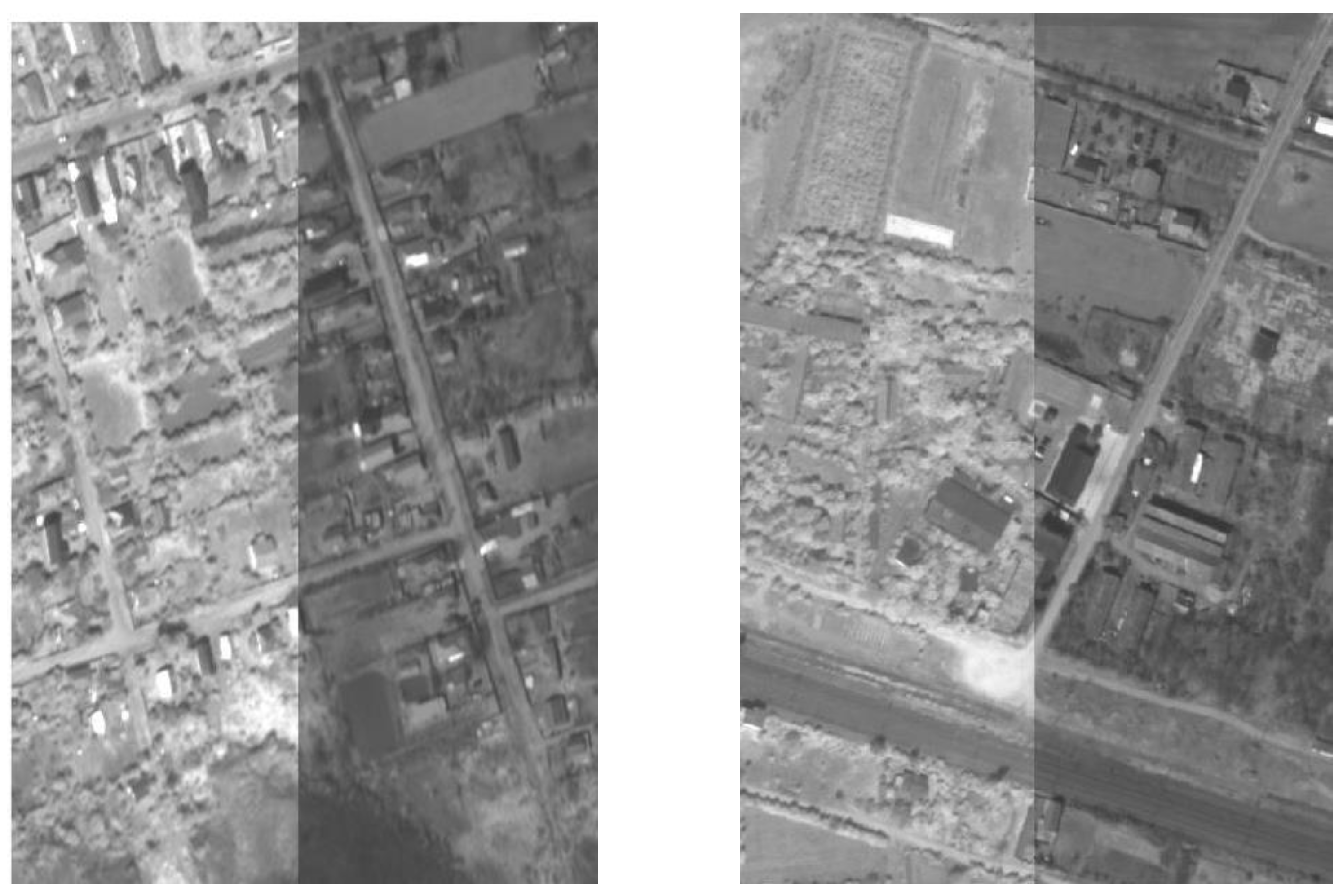
Figure 11.
Sample images showing geometric consistency at a boundary.


Figure 12.
GCP distribution with the number.


Table 1.
Test data specification.
| Product Level | Acquisition Date | Image Size (Pixels) | Incidence/Azimuth | GSD (Col/Row) |
|---|---|---|---|---|
| Strip #1 Level 2R | 4 May 2018 | Sample 24,060 Line 69,946 | 0.75°/79.54° | 0.55/0.55 m |
| Strip #2 Level 2R | 24 April 2018 | Sample 24,060 Line 63,433 | 26.00°/261.58° | 0.67/0.60 m |
| Strip #3 Level 2R | 8 April 2018 | Sample 24,060 Line 71,166 | 11.56°/78.58° | 0.56/0.55 m |
Table 2.
RPCs conversion residual in RMSE (unit: pixels).
| Ephemeris | Strip #1 | Strip #2 | Strip #3 | |||
|---|---|---|---|---|---|---|
| Line | Sample | Line | Sample | Line | Sample | |
| Original | 0.57 | 1.45 | 0.55 | 0.20 | 0.20 | 0.28 |
| Interpolated | 0.11 | 0.10 | 0.10 | 0.07 | 0.20 | 0.10 |
Table 3.
Accuracy of mosaic strip RPCs (unit: pixels).
| RMSE | Max Errors | |||
|---|---|---|---|---|
| Line | Sample | Line | Sample | |
| RPCs of center strip | 4.02 | 40.07 | 6.77 | 45.91 |
| RPCs of Mosaic | 2.88 | 21.07 | 5.51. | 26.78 |
| Accuracy Improvement (%) | 28.4% | 47.4% | 18.6% | 41.7% |
Table 4.
Accuracy of mosaic strip RPCs after the bias compensation (unit: pixels).
| RMSE | Max Errors | |||
|---|---|---|---|---|
| Line | Sample | Line | Sample | |
| Shift | 1.44 | 3.22 | 3.01 | 5.96 |
| Linear | 1.46 | 2.79 | 3.23 | 5.79 |
Publisher’s Note: MDPI stays neutral with regard to jurisdictional claims in published maps and institutional affiliations. |
© 2021 by the authors. Licensee MDPI, Basel, Switzerland. This article is an open access article distributed under the terms and conditions of the Creative Commons Attribution (CC BY) license (https://creativecommons.org/licenses/by/4.0/).
Share and Cite
MDPI and ACS Style
Lee, C.; Oh, J. Sensor-Level Mosaic of Multistrip KOMPSAT-3 Level 1R Products. Appl. Sci. 2021, 11, 6796. https://doi.org/10.3390/app11156796
AMA Style
Lee C, Oh J. Sensor-Level Mosaic of Multistrip KOMPSAT-3 Level 1R Products. Applied Sciences. 2021; 11(15):6796. https://doi.org/10.3390/app11156796
Chicago/Turabian StyleLee, Changno, and Jaehong Oh. 2021. "Sensor-Level Mosaic of Multistrip KOMPSAT-3 Level 1R Products" Applied Sciences 11, no. 15: 6796. https://doi.org/10.3390/app11156796
Note that from the first issue of 2016, this journal uses article numbers instead of page numbers. See further details here.