
A Novel Preprocessing Method for Dynamic Point-Cloud Compression


1
Graduate School of Smart Convergence, Kwangwoon University, Seoul 01897, Korea
2
Department of Electrical Engineering, Kwangwoon University, 20 Kwangwoon-ro, Nowon-gu, Seoul 01897, Korea
3
Ingenium College, Kwangwoon University, Seoul 01897, Korea
*
Author to whom correspondence should be addressed.
Appl. Sci. 2021, 11(13), 5941; https://doi.org/10.3390/app11135941
Submission received: 28 April 2021
/
Revised: 18 June 2021
/
Accepted: 22 June 2021
/
Published: 26 June 2021
(This article belongs to the Special Issue VR/AR/MR with Cloud Computing)
Abstract
:Computer-based data processing capabilities have evolved to handle a lot of information. As such, the complexity of three-dimensional (3D) models (e.g., animations or real-time voxels) containing large volumes of information has increased exponentially. This rapid increase in complexity has led to problems with recording and transmission. In this study, we propose a method of efficiently managing and compressing animation information stored in the 3D point-clouds sequence. A compressed point-cloud is created by reconfiguring the points based on their voxels. Compared with the original point-cloud, noise caused by errors is removed, and a preprocessing procedure that achieves high performance in a redundant processing algorithm is proposed. The results of experiments and rendering demonstrate an average file-size reduction of 40% using the proposed algorithm. Moreover, 13% of the over-lap data are extracted and removed, and the file size is further reduced.
1. Introduction
In recent years, volumetric capture for real-time 3D animation has been focus of research. 3D animation can be represented in the form of dynamic point-clouds or mesh data. Volumetric capture is the creation of dynamic 3D animation data through the capturing of an object with multiple cameras from all directions. Several research groups working on multi-view video-based 3D reconstruction that offer volumetric capture systems worldwide include Mixed Reality Capture Studio [1], 8i [2] and 4D Views [3]. The complete workflow for volume video production based on RGB-D sensors is described in [4]. In [5], the authors proposed a method based on spatial-temporal integration for surface reconstruction using 68 RGB cameras. Their system took 20 min/frame processing time to generate upto three-million faces mesh. Robertini et al. [6] presented an approach focused on improving surface detail by maximizing photo-temporal consistency. Vlasic et al. [7] exploited a complex dynamic lighting system that enabled controllable light and acquisition at a dynamic shape capture pipeline of 240 frames/sec using eight 1024 × 1024 pixel resolution cameras. High quality processing requires processing times of 65 min/frame, however implementations based on a graphic processing unit (GPU) reduced this to achieve 15 min/frame. The use of real-time 3D animation data is widespread in a variety of applications (e.g., game, military, autonomous driving). A large number of resources are used in the process of sending motion data using a raw point-cloud. In general, a dynamic point-cloud has about 10,000 points per frame. In an uncompressed situation, the total bandwidth of 30 fps is 3.6 Gbps [8]. In various research articles, point-cloud simplification is discussed but dynamic point-cloud compression is ignored. There are some volumetric capture studies, such as MS Holopotation, where data acquired in mesh form are studied [9]. In 8i [10], data obtained in the point-cloud form is studied.
In this paper, to reduce the size of continuous point-clouds, we propose a method to convert overlapping vertices between frames into a reusable format, and evaluate the phenomena and results that appear in the conversion process.
2. Background Theory
2.1. Dynamic Point-Cloud
A dynamic point-cloud is 3D animation data composed of point-cloud frames. A point-cloud is one of the 3D data representations that symbolize other captured attributes such as spatial coordinates and colors.
This is a representation of vertex :
It is represented by x, y, z, which indicate spatial coordinates, and c, which indicates color. c is a color composed of the elements r, g, and b.
This is an expression that indicates a point-cloud ():
A point-cloud frame consists of S number of vertices.
This is a representation of a dynamic point-cloud (V):
A dynamic point-cloud consists of T number of point-cloud frames.
Volumetric capture technology digitizes and shoots several real-world objects, including people and backgrounds. These technologies are being studied using multiple rgb and multiple rgb-d cameras. In [11] we see the findings of a multiple rgb camera study. In [12], high-precision research was conducted that minimized the difference from the actual object. In [13,14] we see the findings of a multiple rgb-d camera study. The technology for acquiring real-time 3D models using infrared devices was applied in [15,16,17]. These scanning devices include Zed, LiDAR sensors, etc., other than Kinect. The difference between Kinect and Zed, which scans the front of the device, was studied in [18]. This study made comparisons based on resolution, lighting, accuracy, speed, and memory. The LiDAR (Light Detection and Ranging) sensor, which can scan the area around the device, provides a point-cloud for distance information that measures the travel time of the light emitted to the ToF (time-of-flight) operating principle. This device is often used, especially in applications that measure the surrounding environment [19,20,21]. These scanning technologies can capture real-world movements in multiple frames as digital information.
However, there are problems in measuring full-quality live-action objects in this way. In order to solve these problems, TSDF (truncated surface distance function) technology was applied in [22,23]. A point-cloud is generated for each red-green-blue depth data item acquired through a 3D fusion process that creates a single TSDF volume. To implement points again, the TSDF volumes in multiple scanning devices use a feature point algorithm to quickly digitize a complete real object.
2.2. Point-Cloud Compression
Generally, the acquisition of a large amount of data is necessary, however, the file size then has to be reduced for use in real applications. A single point-cloud is the simplification researched using this method. Simplification is a technology for sampling vertices to reduce the weight of a point-cloud. Currently, commonly used point-cloud simplification methods are the bounding box algorithm [24,25], the uniform grid method [26], the curvature sampling method [27], the clustering method [28], and the triangular grid method [29], etc., [30,31,32,33].
A call for proposals (CfP) was issued in 2017 by the MPEG (Moving Picture Expert Group) for methods for reducing the weight of dynamic point-cloud data [34]. Based on this CfP response, two different compression techniques were selected for point-cloud compression (PCC) standardization activities: geometry-based PCC (G-PCC) [35] and video-based PCC (V-PCC) [36]. G-PCC is a format that expresses a point-cloud in an octree structure. In the octree structure, the point-cloud is assumed to be represented by the range. It means that the vertices are represented by 0 and 1 and divided into 8 voxels of until becomes 1. Advantageously, since the vertices are expressed in 1-byte units instead of being expressed in coordinates, the compression performance is high. Lossy compression and non-lossy compression are determined according to the range of depth bits. V-PCC is a method of compression using an existing video codec. Compression using 2D video compression methods such as the advanced video coding (AVC)/H.264 [37] or high efficiency video coding (HEVC) [38] projects a point-cloud into a 2D space to generate 2D images.
The research undertaken in [39] complements the selected compression technique. In addition, performance evaluation is performed with [40]. However, G-PCC is a compression technology for a single point-cloud, and V-PCC requires a process to generate 2D images in addition to subordinate and complicated process using codec.
3. Proposed Method
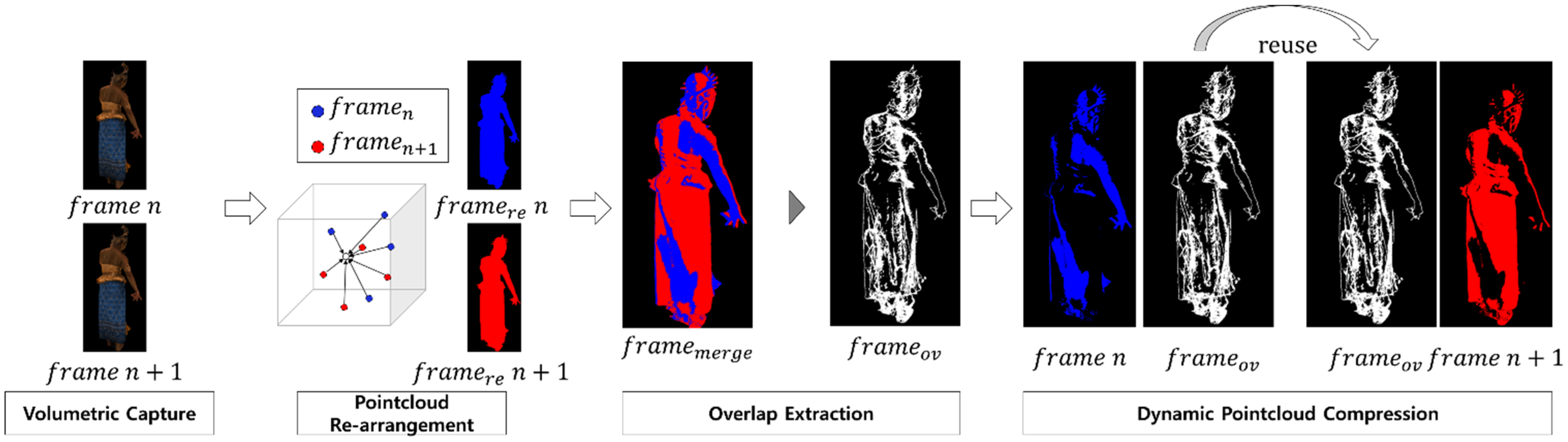
The computing system of this study leverages a pre-processing process to resolve problems appearing in the data, so that redundant information can be efficiently extracted from dynamic point-clouds. Figure 1 shows the entire compression process using the divider algorithm that can remove redundant information, including the proposed pre-processing procedure.
Figure 1 shows the whole system of the proposed method. The suggested pre-processing process have been added prior to the divider process. The pre-processing process converts the existing point-cloud to have a voxel-based data structure.
3.1. Volumetric Capture
In this study, it is assumed that at least two or more point-clouds express and use a series of operations. This procedure refers to the process for acquiring point-cloud raw data. There typically exists both raw data capture and parsing.
General parsing refers to the process of interpreting data defined in a particular format. Among them, point-cloud parsing is commonly used to interpret files. It implies the work of acquiring the recorded point-cloud file with information consisting of raw data such as spatial coordinates and colors. Other methods can be utilized to capture raw data immediately. In the input process provided, the spatial coordinates of the point-cloud are parsed and used. Compression is performed using spatial coordinates, thus work is required to exclude pre-processing colors and other information.
3.2. Point-Cloud Rearrangement
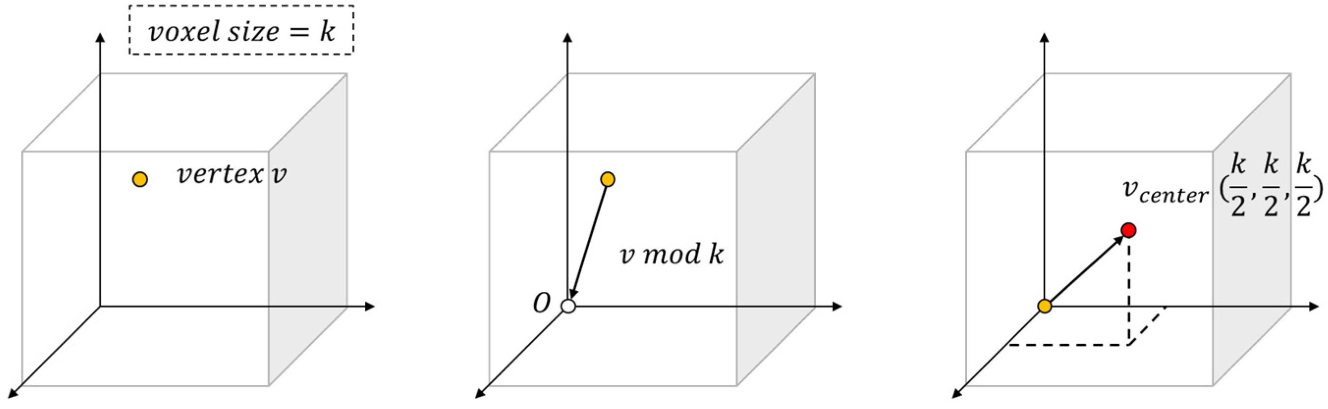
We propose a process to rearrange point-cloud spatial coordinates in voxel units. When using vertex information expressed in real number units, the real number unit has a form in which error values due to devices and algorithms remain. Thus, it is important to rearrange the point-cloud based on the voxel to remove any duplicate vertex. This procedure is shown in the following figure.
Figure 2 demonstrates the point-cloud rearrangement process of the proposed method in order. The box means voxel. The voxel has a size of about , and the voxel is composed of pieces according to the expressed range of the point-cloud. The vertex is represented by the voxel number index and voxel internal coordinates. The range of voxel internal coordinates is from 0 to .
Figure 3a illustrates one of the original point-cloud vertices. Figure 3b shows the result of moving to the point of voxel. The point means the origin of voxel. The relative position of the vertex is obtained by modular operation. Figure 3c indicates the operation of moving the vertex to the center of the voxel. Therefore, the formula for rearrangement of vertex by the proposed method is as follows.
The rearrangement equation proposed in Equation 4 has the result of removing the error by . In other words, if the vertex is data recorded in units of 0.1, it is possible to judge the duplicate vertex even for errors that occur at a value smaller than 0.1 in the = 0.2 and operations.
3.3. Overlap Extraction
This procedure is the process of determining a duplicate vertex by comparing both point-clouds and splitting them into two vertex sets, vertex and . Generally, when comparing two sets where and elements are equal, the method of comparing each set is performed times for data. In this case, it will be repeated times. However, in general, such an operation is not possible in a point-cloud having one million or more elements. Therefore, we use a hash table to compare point-clouds. This hash table consists of an integer-type key and a value in the form of spatial coordinates. Since there is a way to generate spatial coordinates with a key, a point-cloud can be configured with a hash table. When the hash table is used, it is repeated times, so the time used for the comparison operation is greatly reduced.
When performing the overlap extraction for and , which are two point-cloud frames, respectively, it is assumed here that the same vertex does not exist in one point-cloud. First, configure with a hash table. Convert vertex to key format. Perform a duplicate comparison using the hash table of for all key values. The comparison result confirms that each vertex of overlaps with . Divide into when duplicated, and when not.
3.4. Dynamic Point-Cloud Compression
This procedure creates the two acquired sets of vertex, and , in one file. The creation process includes the procedure of combining and to create a compressed point-cloud, . At the stage of generating and recording , an additional value, a difference from the original, is recorded. The value records the mean error of the vertices and indicates the degree of deformation from the source. This information gives a rough indication of the amount of error allowed. The resulting proposed method creates a file so that the overlap between the two point-clouds can be shared.
4. Experimental Environment and Results
4.1. Materials
This section describes the materials used in the proposed method. In this paper, use of the Window10 environment was proposed, and the Unity Game Engine was used to visualize 3D data. Unity Game Engine is a tool that is commonly used for data visualization research. The source for operating the game engine is composed of C # language, within the .Net Framework environment.
The 8iVSLF dataset was used for the experiment. This dataset provides new voxelated high-resolution point-clouds for non-commercial use by the research community as well as test materials for MPEG standardization efforts [41].
Table 1 shows information on data extracted from 8iVSLF data. In this experiment, information from 8iVSLF was extracted and used, excluding 13 types of color and normal data, to obtain accurate results. The extracted point-cloud was written in ASCII format. The number of point-cloud frames used in the experiment is 300.
4.2. Evaluation Method
In the experiment, in addition to the performance evaluation of the proposed method, the amount of change before and after the rearrangement and the simplification performance comparison were additionally analyzed. First, the RMSE value are calculated and the amount of loss depending on voxel size is checked. Additionally, checks are made to verify if the RMSE value has a large image quality difference within the actual rendering environment. The simplification performance confirms the difference in compression ratio and image quality when compared in an environment similar to commercial software. In the simplification comparison experiment, MeshLab’s Simplification function and MatLab’s Sampling function, which are well known as point-cloud editing tools, were used [42]. In this experiment, we obtained 300 point-cloud data, thus there is a limit to how much of the experimental data can be represented. Some evaluation factors were measured from all point-clouds, the maximum value was denoted as Max, the minimum value Min, and the average value of the whole point-cloud Avg. These measurement to calculate the range of error that each point-cloud result can be displayed by the (Max–Min)/Avg calculation. The range of the voxel size used in the experiment records the changes that occur when the voxel size is increased from the minimum distance between the points constituting a point-cloud to twice the maximum distance.
This is the RMSE expression for evaluating the rearrangement performance:
The RMSE value uses a commonly known formula. The source vertex of each vertex of the frame corresponding to the point-cloud frame and the amount of spatial change of the changed vertex are squared and added up. Then, after dividing by the number of vertex, the value of the square root is calculated.
This is the rearrangement cost expression to evaluate the rearrangement performance:
RC (rearrangement cost) is a formula for performance evaluation of the proposed method. It is the value obtained by reconstructing the point-cloud and dividing the total distance traveled by the moving vertex by the number of vertices. This is the average movement of the vertex. In other words, it represents the movement of the point-cloud.
Table 2 shows the rearrangement results by voxel size in terms of the simplification rate. Due to the limitations of representing all experimental data, representative comparison values of 1.26, 1.55, and 2.0 were used, which correspond to levels of 30, 50, and 70% of the text.
4.3. Experimental Results
The experiments are described in the order of the entire compression process. First, the result of experimenting with the original loss during the point-cloud rearrangement process is discussed in Section 4.3.1. After that, simplification performance results are discussed in Section 4.3.2. Finally, the compression result of the proposed method is discussed in Section 4.3.3.
4.3.1. RMSE Results
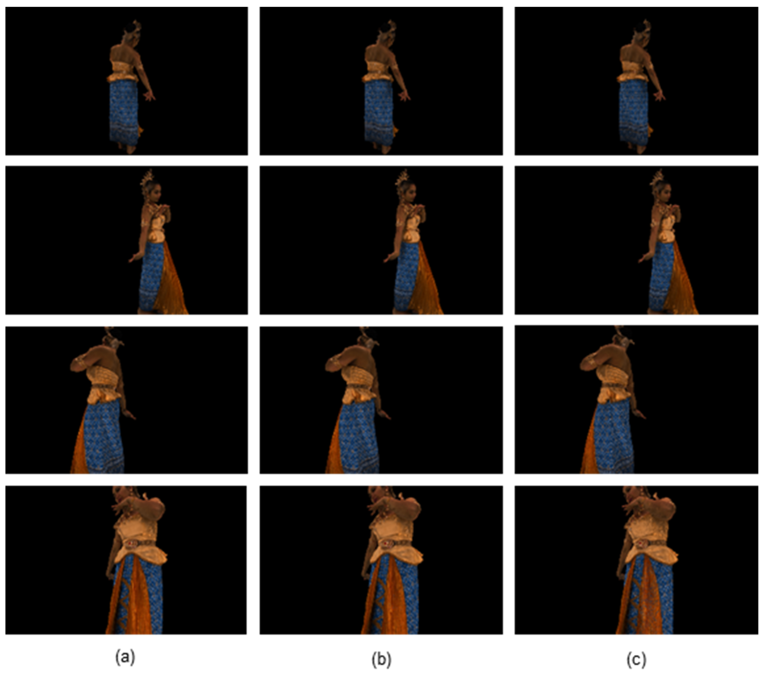
The amount of change in the point-cloud rearrangement result is shown based on the representative voxel size. We measured the RMSE and RC (rearrangement cost) values to show the difference. The following Figure 3 visually displays the rearrangement results.
Since it is difficult to see the difference in visual quality in Figure 3, we will compare the quality in more detail in the next experiment.
Table 3 shows the results of the proposed rearrangement process using the dynamic point-cloud data set, which was measured for both RMSE and RC (rearrangement cost) values.
When the voxel size was 2.0, the experimental result RMSE was measured with an average value of about 1443. This result is equivalent to about 721.8 times the voxel size. The RMSE occurs in the range of about 6.5% (47.45) on average. The average value of RC was about 1.453. This is equivalent to about 72.6% of the voxel size. The RC occurs in the range of about 1.7% (0.01256) on average.
When the voxel size was 1.55, the experimental result RMSE was measured with an average value of about 875. This result is equivalent to about 564.8 times the voxel size. This results is around 21.7% (1–564.8/721.8) less in comparison to the result when the voxel size is 2.0. The RMSE occurs in the range of about 6.0% (26.44) on average. The average value of the RC was about 0.706. This is equivalent to 45.5% of the voxel size. In comparison to the results achieved when the voxel size is 2.0, this is less by about 37.3% (1–45/72). The RC occurs in the range of about 0.4% (0.00145) on average.
When the voxel size was 1.26, the experimental result RMSE was measured with an average value of about 830. This result is equivalent to about 659.0 times the voxel size. This result is higher by about 16.6% (1–564/659) when compared to the results when the voxel size is 1.55. The RMSE occurs in the range of about 6.0% (25.01) on average. The average value of the RC was about 0.564. This is equivalent to about 44% of the voxel size. This result is less by about 1.6% (1–44/45) when compared to the results when the voxel size is 1.55. The RC occurs in the range of about 0.3% (0.00099) on average.
When the voxel size was 2.0, the average point-cloud to RMSE was about 721 times the voxel size, and the RC average was at its highest value, about 72% of the voxel size. When the voxel size was 1.55, the average of the RMSE from point-cloud was measured to be about 564 times the voxel size, and the RC average was measured to be about 45.5% of the voxel size. When the voxel size was 1.26, the average point-cloud to RMSE was measured at about 659 times the voxel size, and the RC average was measured at its lowest value, which was about 44%. Among them, voxel sizes of 1.26 and 1.55 were obtained with a small difference of about 16% in RMSE average and about 1% in RC average.
4.3.2. Simplification Results
An experiment was conducted to compare the original with the modified point-cloud. The values used for the sampling parameters were 30, 50, and 70% of the numbers. The number of vertices in each source point-cloud was used as information to determine the number of data extracted from the source.
Table 4 compares the results of the two traditional methods. The value indicates the file size. The SIM and SAM methods use the number of vertices in the simplification parameter. In the experiment, 30, 50, 70% of the original number of vertices were used. This is the suggested method, where the voxel sizes are respectively 2.0, 1.55, and 1.26.
Measure the Max, Avg, and Min values as described in the experimental method. In addition, the size variation of the simplified file was recorded in the “Dev” item. The results of the smallest size reduction among the SIM, SAM, and PROP methods are displayed in bold.
When the simplification parameter used was 30% (i.e., voxel size = 2.0), the average value showed the best performance in the proposed method. Additionally, the deviation value was 452, which was the lowest result.
When the simplification parameter used was 50% (i.e., voxel size = 1.55), the average value showed the best performance with the MeshLab method. This is about 8% better than the proposed method. The experiment using the MeshLab method showed the highest performance on average, with a deviation of 17,464.
When the simplification parameter used was 70% (i.e., voxel size = 1.26), the mean showed the best performance in the suggested method. In this case, the MeshLab minimum was confirmed, but this method results in higher deviations.
Experiments have shown that the performance of the proposed method is on average high or slightly low. However, the proposed method is less variable than the other methods. This renders it advantageous in handling different shapes. The following figure provides a visual display of the comparison results.
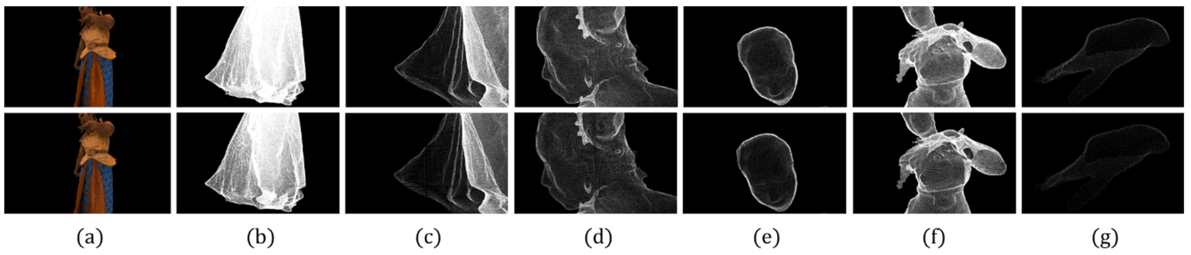
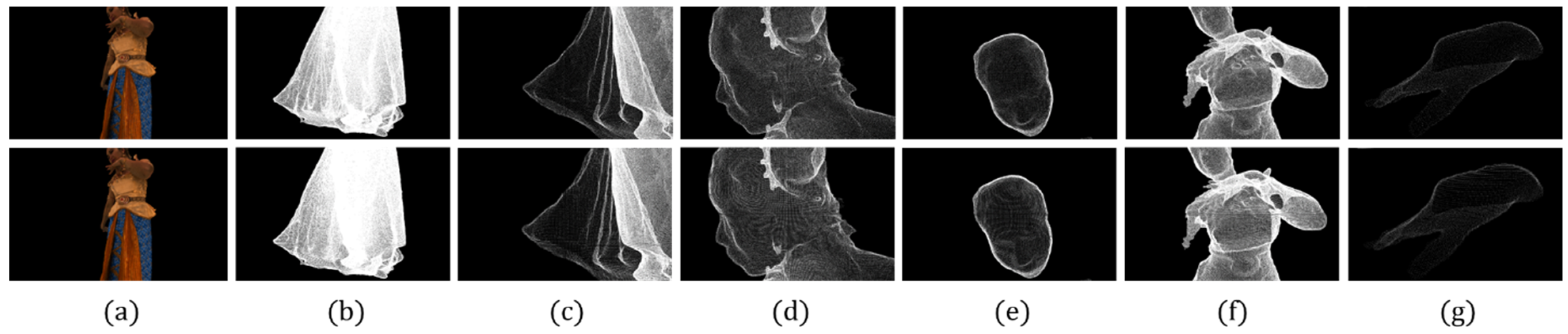
Figure 4 compares the results of experiments with the simplification parameter of a commercially available module at the 30% level. The first line shows the results of the MeshLab simplification. The result of the proposed method is shown on the second line. Figure 3a shows the overall rendering of a point-cloud representing a 2M volume. Figure 3b,c show the thin garment and its detailed results. Figure 3d,e show the body parts that should be represented in detail and their detailed results. Figure 3f,g focus on the areas where the clothing and body are identified together, and the body within which the details must be shown.
This result uses the highest level of simplification parameter. Therefore, many vertices have been removed. However, in Figure 3a, which represents the entire 2M volume, there are no differences in visual quality. In this case, the largest difference appears in Figure 3b. There are clear differences in the part of the human foot in clothes with a spacious and thin volume. Figure 3g also shows the limits of expressing the same narrow, thin volume of the finger.
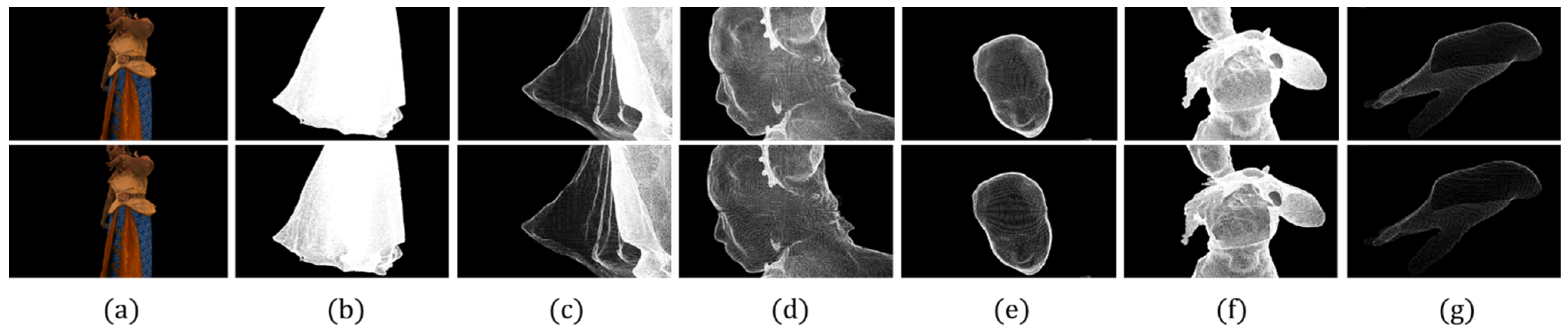
Figure 5 compares the results of experiments with the simplification parameter of a commercially available module at the 50% level. The first line shows the results of the MeshLab simplification. The result of the proposed method is indicated on the second line in Figure 5a. The order of (g) is revealed in Figure 4.
This result demonstrates the differences between Figure 5b,e. As shown in Figure 5b, there is a clear tendency for thick volumes to appear strongly. In Figure 5e, a higher quality image can be observed.
Figure 6 compares the results of experiments with the simplification parameter of a commercially available module at the 70% level. The first line shows the results of the MeshLab simplification. The result of the proposed method is provided on the second line, Figure 6a. The order of (g) is shown in Figure 4.
This result uses the lowest level simplification parameter. Therefore, few vertices have been removed. Most of the vertices are saved in Figure 6b. However, fine leg boundaries are recognizable. Here, instead of the appearance of a thin cloth, as observed with the other simplification parameters, a clear area that is as thick as the body is maintained.
4.3.3. Compression Results
An experiment was conducted to measure the performance of the deduplication algorithm using the point-cloud that was pre-processed using the proposed method (i.e., point transformation). The results of the compression were rendered, checked, and analyzed using the recorded data in this experiment. The results of compression include voxel sizes of 1.26, 1.55, 2.0, which are 30, 50, and 70%, respectively: the same as the parameter values of the conventional method. The result of each voxel size was visualized.
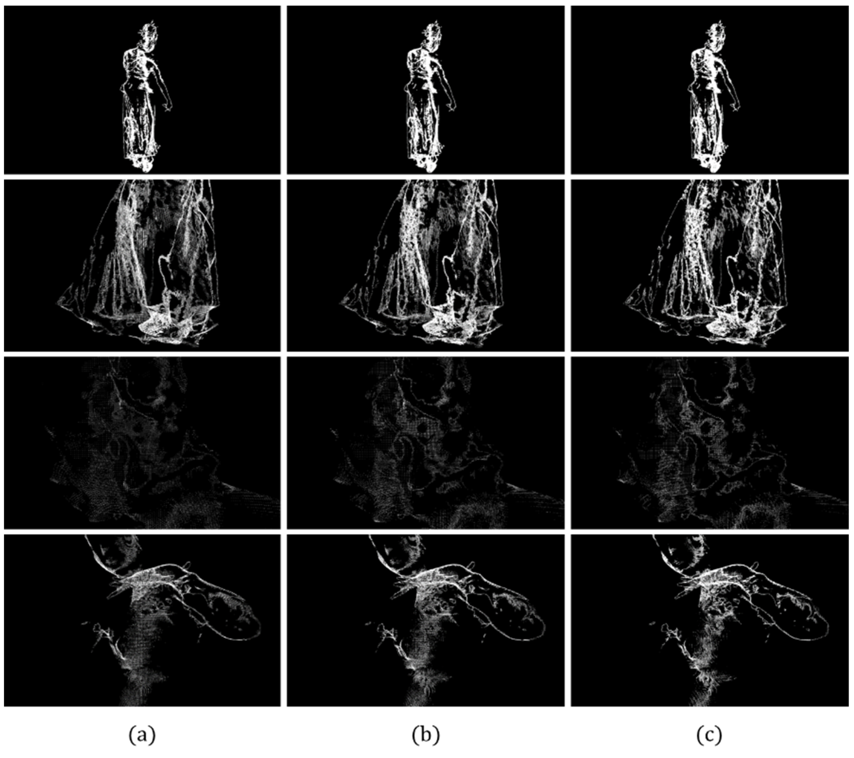
Figure 7 is a visual representation of the duplicate extraction result. The first picture on the left of each row shows the total data for each reference voxel size and the result of comparing more detailed rendering quality in the remaining pictures.
The extracted superposition information was rendered to obtain the results of extracting data similar to the clear outline of the 3D model. The amount of duplicate data extracted gradually increased. However, it proved difficult to determine a distinction with the naked eye. Therefore, the graph in the following figure is the result of an experiment based on voxel size.
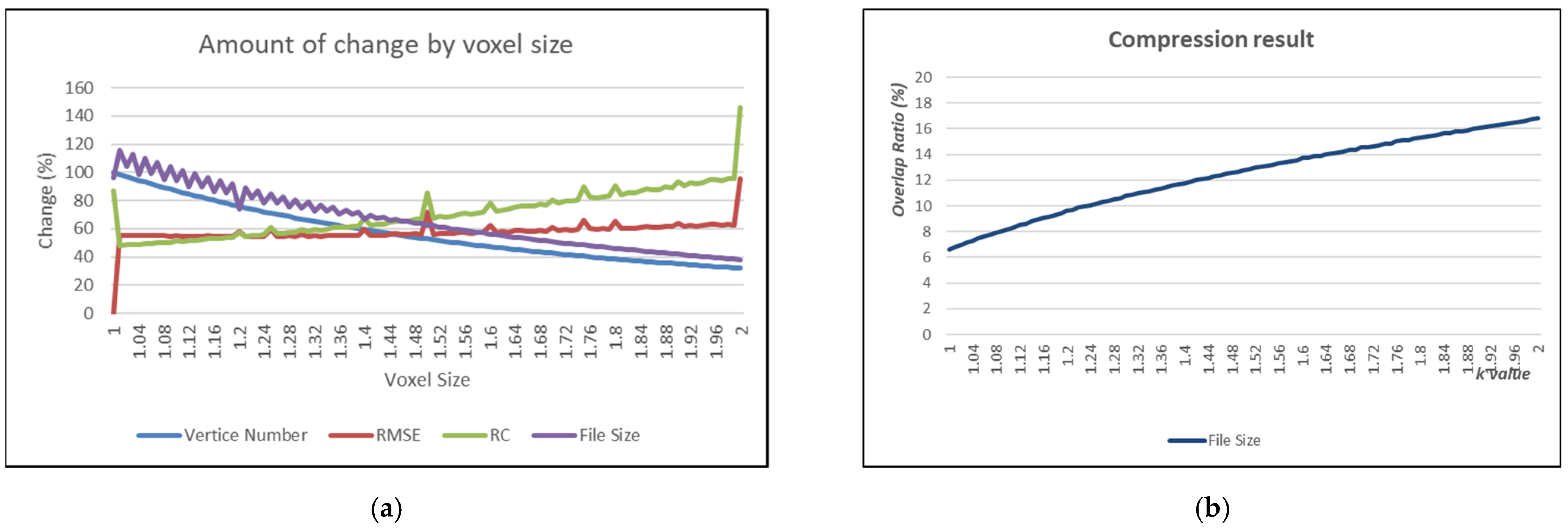
Figure 8 measures the amount of change in the size of the rearranged file according to the voxel size, the number of vertices, RMSE, and RC (rearrangement cost). The vertice number and RMSE correspond to RC and file size, respectively, in Figure 8a. Figure 8b measured the results of the proposed method obtained using the overlapping vertex extraction size between the two point-clouds. Data were recorded in units of 1% of the range of the experiment.
The suggested method uses two point-clouds. Therefore, there is another graph like Figure 8a. In this graph, Figure 8a and the overall data show almost the same level, with a difference of about 0.05%. The vertice number decreases continuously as the voxel size increases, and the RMSE and RC generally increase significantly over a period of time (such as when the voxel size is 1.00, 1.5, or 2.0). File size tends to decrease with repeated slight increases or decreases. This result is reduced to 32% when the voxel size is 2.0.
Figure 8b shows the compression result. The pattern on this graph tends to be linear. The existing 6.63% will increase up to 16.85%.
4.4. Discussion
The rearrangement process is important for the compression process provided. We conducted experiments in two ways to evaluate important algorithms. At first, the amount of loss was measured as the text was deformed. Both RMSE and RC (rearrangement cost) values were measured. We also assessed the simplification results, which measure the additional performance of important algorithms. The best result was achieved using a voxel size of 1.55. We were able to reconstruct the point-cloud efficiently with the least deviation, providing higher or similar file sizes to other methods. Existing simplification algorithms are heavily influenced by the input model and parameters, resulting in high deviations or small deviations and poor performance.
In particular, the RMSE value increased significantly from 0.5, which is the unit that generally constitutes a point-cloud. Measured when the voxel size was 0.5 units (e.g., k = 1.0, 1.5, 2.0) on a dataset with a fixed minimum distance of 1, the proposed algorithm aimed to eliminate chaotic errors. All RMSEs were significantly increased. In general, a certain number of RMSE values are expected to appear in all voxel units in the measured arbitrary dataset.
Finally, we implemented deduplication and conducted an experiment to extract duplicate data using a point-cloud with a preprocessing algorithm. Experimental results were identified by the contours of the 3D model. This is because there was an empty data structure in the point-cloud. It is presumed that the outline shape was generated in the form of a subset of the target frame, because the overlapping vertices of the reference frame of the target contour were extracted. The results extracted using the algorithm were found to increase by 16.85% compared to 6.63% previously when k = 2.0 (i.e., the range of the largest experiment).
5. Conclusions
In this research, we proposed a method to efficiently manage and compress animation information via a 3D point-cloud via experiments using the point conversion method. In particular, a point-cloud preprocessing algorithm for efficiently processing and managing dynamic point-clouds has been proposed. Subtle errors in existing point-clouds are not the right form for duplicate extraction. The proposed method aimed to solve problem by reconfiguring the point-cloud on a voxel basis to eliminate the error. This method repositioned all vertices in the center of the voxel using an expression that converted them to each voxel unit. This result not only eliminated the error, but also removed the unnecessarily high density part from the point-cloud. Checks were undertaken to extract the duplicate vertex of the point-cloud with the error removed in this way. The extracted information was an intersection of both point-clouds. Therefore, this part was shared and used to provide the compression effect. The proposed method showed that the compression ratio increased from 6.63% to 16.85% in proportion to the voxel size when the file was increased to twice the recording unit in which it was created.
In an environment where the 3D model to process is not determined by the real-time system, the maximum and minimum performance are not determined. Therefore, we suggest the use the proposed algorithm instead of the larger algorithm to create a reliable service. As a result of finally compressing the file size twice, we expect that the dynamic point-cloud will be able to be managed efficiently. In addition, 3D model analysis can be implemented using patterns of extracted redundant data that are very close to the outline. The results obtained showed minimal damage to rendering quality and maximum compression when voxel size was 1.55.
The proposed method is expected to be advantageous for compressing point-clouds obtained from different environments and different devices. In particular, as research on acquiring point-clouds on mobile devices with strong device-specific characteristics progresses, it is expected that this method can be applied to easily implement compression. However, more detailed research between compression performance and quality is needed in the future. In this experiment, voxel size was analyzed intensively as a representative. In addition, various voxel sizes need to be studied.
Author Contributions
Conceptualization, M.-y.L. and S.-c.K.; methodology, M.-y.L.; software, M.-y.L.; validation, S.-h.L. (Sang-ha Lee); formal analysis, M.-y.L. and S.-h.L. (Seung-hyun Lee); investigation, S.-h.L. (Sang-ha Lee) and K.-d.J.; resources, S.-h.L. (Sang-ha Lee) and S.-h.L. (Seung-hyun Lee); data curation, M.-y.L.; writing—original draft preparation, M.-y.L. and S.-c.K.; visualization, M.-y.L. and S.-c.K.; supervision, S.-c.K. and K.-d.J.; project administration, S.-c.K. and K.-d.J. All authors have read and agreed to the published version of the manuscript.
Funding
This research received no external funding.
Institutional Review Board Statement
Not applicable.
Informed Consent Statement
Not applicable.
Data Availability Statement
The data presented in this study are available on request from the corresponding author. The data are not publicly available due to privacy reasons.
Acknowledgments
This work was supported by Institute of Information & Communications Technology Planning & Evaluation (IITP) grant funded by the Korean government (MSIT) (No.2020-0-00192, AR Cloud, Anchor, Augmented Reality, Fog Computing, Mixed Reality).
Conflicts of Interest
The authors declare no conflict of interest.
References
- Available online: https://www.microsoft.com/en-us/mixed-reality/capture-studios (accessed on 25 June 2021).
- Available online: https://8i.com/ (accessed on 25 June 2021).
- 4D View Solutions, [Online]. Available online: http://www.4dviews.com (accessed on 25 June 2021).
- Collet, A.; Chuang, M.; Sweeney, P.; Gillett, D.; Evseev, D.; Calabrese, D.; Hoppe, H.; Kirk, A.G.; Sullivan, S. High-quality streamable free-viewpoint video. ACM Trans. Graph. 2015, 34, 1–13. [Google Scholar] [CrossRef]
- Leroy, V.; Franco, J.-S.; Boyer, E. Multi-view Dynamic Shape Refinement Using Local Temporal Integration. In Proceedings of the 2017 IEEE International Conference on Computer Vision (ICCV), Venice, Italy, 22–29 October 2017; pp. 3113–3122. [Google Scholar]
- Robertini, N.; Casas, D.; De Aguiar, E.; Theobalt, C. Multi-view Performance Capture of Surface Details. Int. J. Comput. Vis. 2017, 124, 96–113. [Google Scholar] [CrossRef] [Green Version]
- Vlasic, D.; Peers, P.; Baran, I.; Debevec, P.; Popović, J.; Rusinkiewicz, S.; Matusik, W. Dynamic shape capture using multi-view photometric stereo. ACM Trans. Graph. 2009, 28, 1–11. [Google Scholar] [CrossRef]
- Graziosi, D.; Nakagami, O.; Kuma, S.; Zaghetto, A.; Suzuki, T.; Tabatabai, A. An overview of ongoing point cloud compression standardization activities: Video-based (V-PCC) and geometry-based (G-PCC). APSIPA Trans. Signal Inf. Process. 2020, 9. [Google Scholar] [CrossRef] [Green Version]
- Wang, P.; Bai, X.; Billinghurst, M.; Zhang, S.; Zhang, X.; Wang, S.; He, W.; Yan, Y.; Ji, H. AR/MR Remote Collaboration on Physical Tasks: A Review. Robot. Comput. Manuf. 2021, 72, 102071. [Google Scholar] [CrossRef]
- Cui, Y.; Chen, R.; Chu, W.; Chen, L.; Tian, D.; Li, Y.; Cao, D. Deep Learning for Image and Point Cloud Fusion in Autonomous Driving: A Review. IEEE Trans. Intell. Transp. Syst. 2021. [Google Scholar] [CrossRef]
- Schenk, T. Introduction to Photogrammetry; The Ohio State University: Columbus, OH, USA, 2005. [Google Scholar]
- Shahbazi, M.; Sohn, G.; Théau, J.; Menard, P. Development and Evaluation of a UAV-Photogrammetry System for Precise 3D Environmental Modeling. Sensors 2015, 15, 27493–27524. [Google Scholar] [CrossRef] [Green Version]
- Rusu, R.B.; Cousins, S. 3d is here: Point cloud library (pcl). In Proceedings of the 2011 IEEE International Conference on Robotics and Automation, Shanghai, China, 9–13 May 2011; pp. 1–4. [Google Scholar]
- Khoshelham, K. Accuracy analysis of kinect depth data. ISPRS Int. Arch. Photogramm. Remote. Sens. Spat. Inf. Sci. 2012, XXXVIII-5, 133–138. [Google Scholar] [CrossRef] [Green Version]
- Chan, T.O.; Lichti, D.D.; Jahraus, A.; Esfandiari, H.; Lahamy, H.; Steward, J.; Glanzer, M. An Egg Volume Measurement System Based on the Microsoft Kinect. Sensors 2018, 18, 2454. [Google Scholar] [CrossRef] [Green Version]
- Sun, G.; Wang, X. Three-Dimensional Point Cloud Reconstruction and Morphology Measurement Method for Greenhouse Plants Based on the Kinect Sensor Self-Calibration. Agronomy 2019, 9, 596. [Google Scholar] [CrossRef] [Green Version]
- Robinson, M.; Parkinson, M. Estimating anthropometry with microsoft kinect. In Proceedings of the 2nd International Digital Human Modeling Symposium, Ann Arbor, MI, USA, 11–13 June 2013; Volume 1. [Google Scholar]
- Gupta, T.; Li, H. Indoor mapping for smart cities—An affordable approach: Using Kinect Sensor and ZED stereo camera. In Proceedings of the 2017 International Conference on Indoor Positioning and Indoor Navigation (IPIN), Sapporo, Japan, 18–21 September 2017; pp. 1–8. [Google Scholar]
- Maksymova, I.; Steger, C.; Druml, N. Review of LiDAR Sensor Data Acquisition and Compression for Automotive Applications. Proceedings 2018, 2, 852. [Google Scholar] [CrossRef] [Green Version]
- Jansson, S.; Malmqvist, E.; Mlacha, Y.; Ignell, R.; Okumu, F.; Killeen, G.; Kirkeby, C.; Brydegaard, M. Real-time dispersal of malaria vectors in rural Africa monitored with lidar. PLoS ONE 2021, 16, e0247803. [Google Scholar] [CrossRef]
- Mäyrä, J.; Keski-Saari, S.; Kivinen, S.; Tanhuanpää, T.; Hurskainen, P.; Kullberg, P.; Poikolainen, L.; Viinikka, A.; Tuominen, S.; Kumpula, T.; et al. Tree species classification from airborne hyperspectral and LiDAR data using 3D convolutional neural networks. Remote. Sens. Environ. 2021, 256, 112322. [Google Scholar] [CrossRef]
- Kim, H.; Lee, B. Probabilistic TSDF Fusion Using Bayesian Deep Learning for Dense 3D Reconstruction with a Single RGB Camera. In Proceedings of the 2020 IEEE International Conference on Robotics and Automation (ICRA), Paris, France, 31 May–31 August 2020; pp. 8623–8629. [Google Scholar]
- Boyko, A.I.; Matrosov, M.P.; Oseledets, I.V.; Tsetserukou, D.; Ferrer, G. TT-TSDF: Memory-Efficient TSDF with Low-Rank Tensor Train Decomposition. In Proceedings of the 2020 IEEE/RSJ International Conference on Intelligent Robots and Systems (IROS), Las Vegas, NV, USA, 25–29 October 2020; pp. 10116–10121. [Google Scholar]
- Sun, W.; Bradley, C.; Zhang, Y.; Loh, H. Cloud data modelling employing a unified, non-redundant triangular mesh. Comput. Des. 2001, 33, 183–193. [Google Scholar] [CrossRef]
- Weir, D.J.; Milroy, M.; Bradley, C. Reverse engineering physical models empolying wrap-aroud B-spline surfaces and quadrics. J. Eng. Manuf. 1996, 210, 147–157. [Google Scholar] [CrossRef]
- Martin, R.R.; Stroud, I.A.; Marshall, A.D. Data reduction for reverse engineering. Proc. Inf. Geometers Conf. 1997, 10, 85–100. [Google Scholar]
- Kim, S.-J.; Kim, C.-H.; Levin, D. Surface simplification using a discrete curvature norm. Comput. Graph. 2002, 26, 657–663. [Google Scholar] [CrossRef]
- Zhao, P.; Wang, Y.; Hu, Q. A feature preserving algorithm for point cloud simplification based on hierarchical clustering. In Proceedings of the 2016 IEEE International Geoscience and Remote Sensing Symposium (IGARSS), Beijing, China, 10–15 July 2016; pp. 5581–5584. [Google Scholar]
- Chen, Y.H.; Ng, C.; Wang, Y. Data reduction in integrated reverse engineering and rapid prototyping. Int. J. Comput. Integr. Manuf. 1999, 12, 97–103. [Google Scholar] [CrossRef]
- Han, H.; Han, X.; Sun, F.; Huang, C. Point cloud simplification with preserved edge based on normal vector. Opt. 2015, 126, 2157–2162. [Google Scholar] [CrossRef]
- Tonini, M.; Abellán, A. Rockfall detection from terrestrial LiDAR point clouds: A clustering approach using R. J. Spat. Inf. Sci. 2014, 8, 95–110. [Google Scholar] [CrossRef]
- Chen, Z.; Da, F. 3D point cloud simplification algorithm based on fuzzy entropy iteration. Acta Opt. Sinica 2013, 33, 0815001. [Google Scholar] [CrossRef]
- Turk, G. Texture synthesis on surfaces. In Proceedings of the 28th Annual Conference on Computer Graphics and Interactive Techniques—SIGGRAPH ’01, Los Angeles, CA, USA, 12–17 August 2001; ACM: New York, NY, USA; pp. 347–354. [Google Scholar] [CrossRef]
- MPEG 3DG, Call for Proposals for Point Cloud Compression v2. Available online: https://mpeg.chiariglione.org/standards/mpeg-i/point-cloud-compression/call-proposals-point-cloud-compression (accessed on 20 June 2021).
- Zakharchenko, V. V-PCC Codec Description. Available online: https://mpeg.chiariglione.org/standards/mpeg-i/geometry-based-point-cloud-compression/g-pcc-codec-description-v2 (accessed on 20 June 2021).
- G-PCC Codec Description v2; ISO/IEC JTC1/SC29/WG11 N18189. 2019. Available online: https://committee.iso.org/home/jtc1sc29 (accessed on 20 June 2021).
- Series, H. Audiovisual and Multimedia Systems, Infrastructure of Audiovisual Services—Coding of Moving Video, Advanced Video Coding for Generic Audiovisual Services; International Telecommunication Union: Geneva, Switzerland, 2003; p. 131. [Google Scholar]
- Coding, High Efficiency Video. Version 1, Rec. Available online: https://www.itu.int/rec/T-REC-H.265 (accessed on 20 June 2021).
- Graziosi, D.; Tabatabai, A.; Zakharchenko, V.; Zaghetto, A. V-PCC Component Synchronization for Point Cloud Reconstruction. In Proceedings of the 2020 IEEE 22nd International Workshop on Multimedia Signal Processing (MMSP), Tampere, Finland, 21–24 September 2020; pp. 1–5. [Google Scholar]
- Guede, C.; Andrivon, P.; Marvie, J.-E.; Ricard, J.; Redmann, B.; Chevet, J.-C. V-PCC Performance Evaluation of the First MPEG Point Codec. SMPTE Motion Imaging J. 2021, 130, 36–52. [Google Scholar] [CrossRef]
- MPEG Point Cloud Compression. Available online: https://mpeg-pcc.org/index.php/pcc-content-database/8i-voxelized-surface-light-field-8ivslf-dataset/ (accessed on 27 May 2021).
- Cignoni, P.; Callieri, M.; Corsini, M.; Dellepiane, M.; Ganovelli, F.; Ranzuglia, G. Meshlab: An open-source mesh processing tool. In Proceedings of the Eurographics Italian Chapter Conference, Salerno, Italy, 2–4 July 2008; pp. 129–136. [Google Scholar]
Figure 1.
Visualization of the compression process provided.

Figure 2.
Visualization of rearrangement procedure.

Figure 3.
Data changes according to voxel size (k) and the rendering results for each: (a) k = 1.26, (b) k = 1.55, and (c) k = 2.0.
Figure 3.
Data changes according to voxel size (k) and the rendering results for each: (a) k = 1.26, (b) k = 1.55, and (c) k = 2.0.

Figure 4.
Comparison of the quality of the results of voxel size k = 2.0 of the proposed method: (a) whole body, (b) skirt, (c) detailed skirt, (d) head, (e) face, (f) whole surface and (g) hand.
Figure 4.
Comparison of the quality of the results of voxel size k = 2.0 of the proposed method: (a) whole body, (b) skirt, (c) detailed skirt, (d) head, (e) face, (f) whole surface and (g) hand.

Figure 5.
Comparing the quality of the results of voxel size k = 1.55 of the proposed method: (a) whole body, (b) skirt, (c) detailed skirt, (d) head, (e) face, (f) whole surface and (g) hand.
Figure 5.
Comparing the quality of the results of voxel size k = 1.55 of the proposed method: (a) whole body, (b) skirt, (c) detailed skirt, (d) head, (e) face, (f) whole surface and (g) hand.

Figure 6.
Comparison of the quality of the results of voxel size k = 1.26 of the proposed method: (a) whole body, (b) skirt, (c) detailed skirt, (d) head, (e) face, (f) whole surface and (g) hand.
Figure 6.
Comparison of the quality of the results of voxel size k = 1.26 of the proposed method: (a) whole body, (b) skirt, (c) detailed skirt, (d) head, (e) face, (f) whole surface and (g) hand.

Figure 7.
Rendering overlap extraction data of the divider algorithm according to voxel size change: (a) k = 1.25, (b) k = 1.55, and (c) k = 2.0.
Figure 7.
Rendering overlap extraction data of the divider algorithm according to voxel size change: (a) k = 1.25, (b) k = 1.55, and (c) k = 2.0.

Figure 8.
Data correlation graph according to voxel size change: (a) amount of change by voxel size; (b) compression result.
Figure 8.
Data correlation graph according to voxel size change: (a) amount of change by voxel size; (b) compression result.


Table 1.
Dynamic point-cloud extraction results.
| Categories | 8iVSLF | Extracting Dynamic Point-cloud | ||
|---|---|---|---|---|
| File Size | Vertex | File Size | Vertex | |
| MAX | 546,953 | 3,205,624 | 92,023 | 3,205,624 |
| AVG | 509,690 | 3,203,001 | 85,153 | 3,203,001 |
| MIN | 486,148 | 3,197,804 | 38,491 | 3,197,804 |
Table 2.
Voxel-size approximation values.
| Voxel Size (k) | Compression Ratio (%) |
|---|---|
| 1.25 | 71.23 |
| 1.26 | 70.35 |
| 1.27 | 69.47 |
| 1.54 | 50.56 |
| 1.55 | 49.99 |
| 1.56 | 49.42 |
| 1.99 | 32.36 |
| 2.0 | 32.08 |
Table 3.
RMSE results according to voxel size.
| Categories | ||||||
|---|---|---|---|---|---|---|
| RC | RC | RC | ||||
| MAX | 1506 | 1.468 | 908 | 0.707 | 861 | 0.565 |
| AVG | 1443 | 1.453 | 875 | 0.706 | 830 | 0.564 |
| MIN | 1411 | 1.443 | 855 | 0.704 | 811 | 0.563 |
Table 4.
Simplification result comparison table (unit: Kb).
| Categories | 30% (k = 2.0) | 50% (k = 1.55) | 70% (k = 1.26) | ||||||
|---|---|---|---|---|---|---|---|---|---|
| SIM | SAM | PROP | SIM | SAM | PROP | SIM | SAM | PROP | |
| Max | 42,311 | 36,575 | 22,263 | 88,216 | 60,957 | 54,061 | 90,648 | 85,341 | 69,241 |
| Avg | 36,426 | 38,252 | 20,647 | 46,556 | 63,753 | 50,205 | 83,711 | 89,254 | 64,308 |
| Min | 20,017 | 41,161 | 19,733 | 36,557 | 68,600 | 47,956 | 37,841 | 96,041 | 61,498 |
| Dev | 7014 | 828 | 452 | 17,464 | 1381 | 1099 | 4955 | 1933 | 1413 |
Publisher’s Note: MDPI stays neutral with regard to jurisdictional claims in published maps and institutional affiliations. |
© 2021 by the authors. Licensee MDPI, Basel, Switzerland. This article is an open access article distributed under the terms and conditions of the Creative Commons Attribution (CC BY) license (https://creativecommons.org/licenses/by/4.0/).
Share and Cite
MDPI and ACS Style
Lee, M.-y.; Lee, S.-h.; Jung, K.-d.; Lee, S.-h.; Kwon, S.-c. A Novel Preprocessing Method for Dynamic Point-Cloud Compression. Appl. Sci. 2021, 11, 5941. https://doi.org/10.3390/app11135941
AMA Style
Lee M-y, Lee S-h, Jung K-d, Lee S-h, Kwon S-c. A Novel Preprocessing Method for Dynamic Point-Cloud Compression. Applied Sciences. 2021; 11(13):5941. https://doi.org/10.3390/app11135941
Chicago/Turabian StyleLee, Mun-yong, Sang-ha Lee, Kye-dong Jung, Seung-hyun Lee, and Soon-chul Kwon. 2021. "A Novel Preprocessing Method for Dynamic Point-Cloud Compression" Applied Sciences 11, no. 13: 5941. https://doi.org/10.3390/app11135941
Note that from the first issue of 2016, this journal uses article numbers instead of page numbers. See further details here.