Review

On Finding the Right Sampling Line Height through a Parametric Study of Gas Dispersion in a NVB

1
Department of Engineering for Livestock Management, Leibniz Institute for Agricultural Engineering and Bioeconomy, 14469 Potsdam, Germany
2
Department of Civil and Architectural Engineering-Design and Construction, Aarhus University, 8000 Aarhus C, Denmark
3
Department of Veterinary Medicine, Institut of Animal Hygiene and Environmental Health, Freie Universität, 14163 Berlin, Germany
4
Hermann-Rietschel-Institut, Chair of Building Energy Engineering, Technische Universität, 10587 Berlin, Germany
*
Author to whom correspondence should be addressed.
Appl. Sci. 2021, 11(10), 4560; https://doi.org/10.3390/app11104560
Submission received: 7 March 2021 / Revised: 13 April 2021 / Accepted: 26 April 2021 / Published: 17 May 2021

Abstract

:
The tracer gas method is one of the common ways to evaluate the air exchange rate in a naturally ventilated barn. One crucial condition for the accuracy of the method is that both considered gases (pollutant and tracer) are perfectly mixed at the points where the measurements are done. In the present study, by means of computational fluids dynamics (CFD), the mixing ratio NH 3 /CO 2 is evaluated inside a barn in order to assess under which flow conditions the common height recommendation guidelines for sampling points (sampling line and sampling net) of the tracer gas method are most valuable. Our CFD model considered a barn with a rectangular layout and four animal-occupied zones modeled as a porous medium representing pressure drop and heat entry from lying and standing cows. We studied three inflow angles and six combinations of air inlet wind speed and temperatures gradients covering the three types of convection, i.e., natural, mixed, and forced. Our results showed that few cases corresponded to a nearly perfect gas mixing ratio at the currently common recommendation of at least a 3 m measurement height, while the best height in fact lied between 1.5 m and 2.5 m for most cases.

1. Introduction

Gas emissions from natural ventilated barns (NVBs) are often estimated using the tracer gas method, which relies on the assumption that the tracer and target gas are well mixed at the location of measurement (e.g., for CO 2 balancing where CO 2 is a naturally produced tracer) [1]. Measurement uncertainty is high since gas mixing is not perfect [2]. Line measurements with sample points every 10 m are typically used to reduce the uncertainty, but there is no general recommendation on the measurement points’ height [3]. The VERA test protocol [4], which is a guideline on the measurement strategy for naturally ventilated buildings, recommends a height of at least three meters for the sampling lines. These guidelines were formulated based on expert rating of common flow conditions; however, environmental conditions are not constant in and around real NVBs, and different farms have specific building characteristics. This situation leads to the fact that, under on-farm conditions, systematic investigation of the impact of changing boundary conditions on indoor climate and emissions is rather difficult. In this context, parametric studies with validated computational fluid dynamics (CFD) models can help to fill this gap and gain better understanding of the general gas emission pattern. Drewry et al. [5] found that the flow convection type (natural, mixed, forced) affects the gas concentrations and temperature distribution. Further investigations are needed to deepen the understanding of those kinds of impacts. With Reynolds-averaged Navier–Stokes (RANS) simulations, reasonable computing times can be achieved, but the right choice of the turbulent Schmidt number is essential to derive a meaningful gas emission pattern.
The turbulent Schmidt number (Sct-number), which is the ratio of momentum diffusivity to mass diffusivity, plays an essential role in the numerical RANS modeling of gas dispersion in CFD. As was reminded in Blocken et al. [6] and confirmed in the present work, the influence of the turbulent Schmidt number on gas dispersion simulations is huge. The main reason for this is that, as will be detailed in Section 2.2.4, in the RANS equations, the coefficient influencing the gas dispersion is not interpreted by the solver, but is given by the user. Thus, an appropriate selection of the Sct-number is crucial to derive meaningful recommendations for practical measurements from the CFD model. Research has been done in order to find the ways and methods for a systematic determination of the turbulent Schmidt number. The results of the studies showed that many factors influence the turbulent Schmidt number such as the flow medium (for example, air or water) and the flow conditions (for example, close or open space). The review paper of Gualtieri [7] summarized the recent research done on the topic of environmental flows using the CFD method. The review pictured a range of Sct-number values for dispersion phenomena used in both air and water systems. He also concluded the impossibility of identifying a universal Sct acceptable for all the diverse flow cases. Drewry et al. [5] did the CFD model validation with Sct = 0.6 based on experimental methane and ammonia emissions from one cow. However, the work focused on the effects of buoyancy flow in a closed space, and the effect of the turbulent Schmidt number on the gas dispersion has not been explored. Gromke et al. [8] studied the gas dispersion in a street canyon with trees by means of a wind tunnel and numerical investigations. He varied the value of the Sct-number from 0.2 to one and found that Sct = 0.3 best matched the experiments data. Gorle et al. [9], in order to predict the dispersion in the wake of a rectangular building, found and applied a Sct-number depending on the RANS turbulence model k-epsilon constants, C o and C μ . However, the results were not satisfactory with a high discrepancy between the experiments and the numerical model. Through this literature review, it can be concluded that the safest way to find the appropriate Sct-number for RANS simulations is through empirical methods.
For this reason, we dedicated the first part of this study to finding the suitable Sct-number of the CFD RANS model that reflects the realistic dispersion pattern observed in a wind tunnel pre-study. This part also highlighted the limitations of the RANS model with regard to the transferability of simulated data for the planning and interpretation of real-scale measurements. In the second part, parameter (such as the inlet flow directions, convection scheme) studies on a naturally ventilated dairy barn were conducted with the validated CFD RANS model. The goal here was to investigate the influence of the height of sampling points inside the barn on the evaluation of the gas mixing ratio between the tracer (CO 2 from animals’ respiration) and the target gas (NH 3 from animal manure). We tested the following hypothesis: the buoyancy effects (through the Richardson number) and wind direction have a significant impact on the tracer-target ratio at commonly used sampling positions.
The goal of this paper was consequently to evaluate, with the help of numerical flow analysis, under which flow conditions common height recommendation guidelines for sampling points of the tracer gas method are most valuable. We further investigated whether there was an added value of considering a planar measurement net in comparison with the common measurement lines.

2. Materials and Methods

2.1. Wind Tunnel Measurements

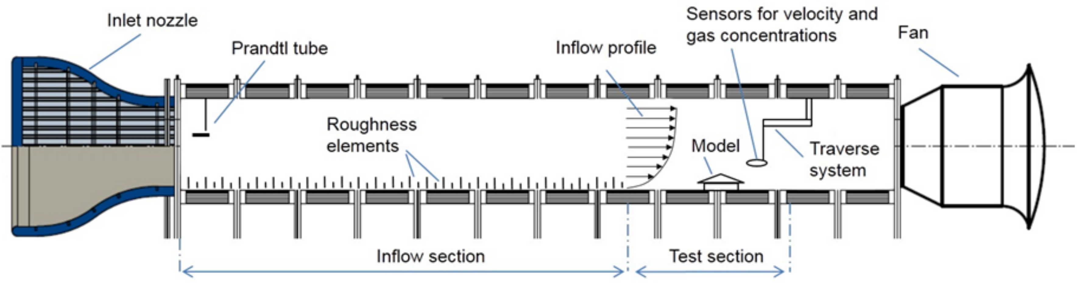
2.1.1. The Wind Tunnel in General

Experimental airflow and gas concentration measurements were obtained on a scale of 1:100 in the atmospheric boundary layer wind tunnel (ABLWT) at ATB (Figure 1) [10]. Within the wind tunnel, a fully developed turbulent flow with a power law vertical velocity profile was generated by the presence of roughness elements at the inflow section. The inflow profile fulfilled the criteria for a boundary layer over a moderately rough terrain according to VDI (2000). The vertical inlet velocity profile was measured using a 2D fiber-optic laser Doppler anemometer (LDA) (Dantec Dynamics, Skovlunde, Denmark) combined with the BSA Flow Software package (Dantec Dynamics, Skovlunde, Denmark). Ethane, i.e., C 2 H 6 , gas dispersion was measured using a fast flame ionization detector (FFID). For more details, we refer to Janke et al. [10].

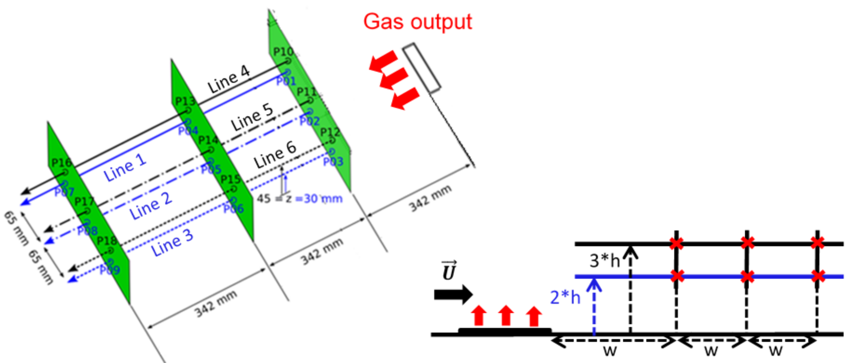
2.1.2. Velocity, Gas Source Characteristics, and Sampling Positions of the Gas

In our case, an undisturbed inlet velocity of 8 m s 1 was used. After preliminary studies, the value of 320 normal liters per hour with the composition of 80% ethane/20% air was injected from a gas diffusor, consisting of a porous stone material (Marina Extendable Airstone, HAGEN GROUP, Germany), which ensured a uniform release of the gas over the surface, mimicking an emission active surface. Ethane was chosen as the tracer gas since its density is close to air’s density, facilitating the transport of ethane by air flow since the effect of gravity is reduced.
The concentrations of ethane were measured at a total of 18 points. The design of the point positions is presented in Figure 2. Three aligned points formed one horizontal line in the flow direction. In Table 1, it is recalled which points correspond to which lines. The points forming Lines 1, 2, and 3 were placed at a height of 2·h (h = 15 mm, with reference to a 1:100 scaled standing cow height). The points forming Lines 4, 5, and 6 were placed at a height of 3·h. While there was no NVB in the wind tunnel setup, the distances of the measurement locations were chosen to correspond to the typical dimensions of the NVB with a ~35 m width.

2.2. CFD Validation for Gas Dispersion

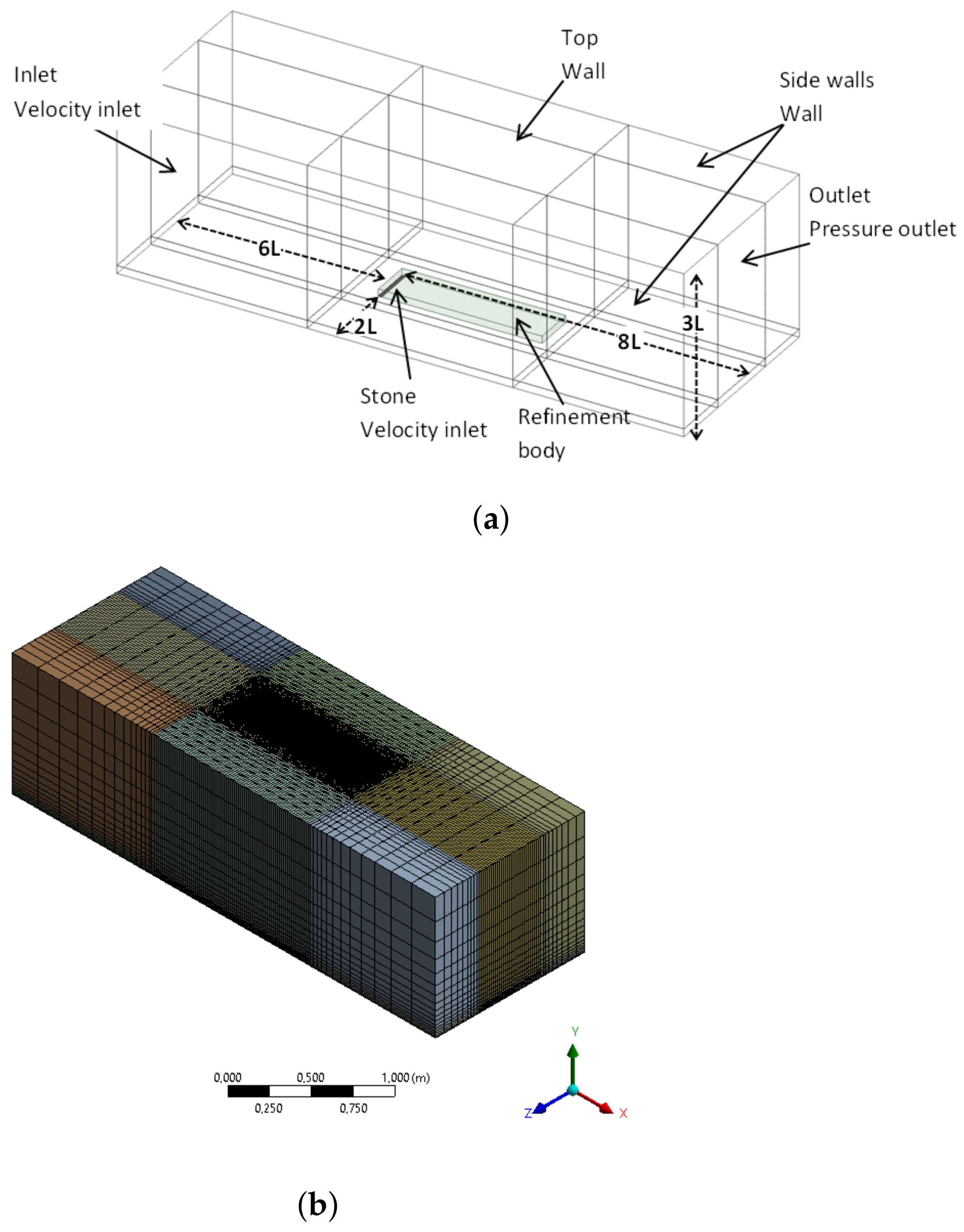
2.2.1. Domain Dimension and Boundary Conditions

The stone was designed as an empty space inside a computational domain. At top of the stone was assigned the boundary condition of the gas output velocity inlet. The dimensions for the domain were chosen according to Marco Lanfrit [11], so that the influences of the side walls and top on the flow could be neglected. The domain dimensions are summarized in Figure 3.

2.2.2. Grid Independence

In order to have control of the mesh, the domain was divided into blocs. The same method was used in Doumbia et al. [12]. The advantage of this method is the economy in the number of cells, allowing thus faster computation. A mesh convergence study was done with three different mesh cell numbers, coarse (1,158,870 cells), mid (2,728,878 cells), and fine mesh (3,319,102 cells). We call C i , c o , C i , m i , and C i , f i (in kg m 3 ) the concentrations at the point i for each coarse, mid, and fine mesh, respectively. The mesh convergence study was done with the k-omega model for a Sct-number of 0.7. The difference of the average concentration of all points in terms of percentage between the coarse and the mid mesh 1 / 18 · i = 01 18 C i , c o C i , m i d / ( C i , c o · 100 ) was equal to 26.6%. The same comparison between the mid and the fine mesh 1 / 18 · i = 01 18 C i , m i d C i , f i / ( C i , m i d · 100 ) was equal to 5.8% (see Table 2). Due to the minimum difference between the mid mesh and the fine mesh, the mid mesh was retained for the rest of the study. Details about the mid mesh are given in the following. The cell size for the block containing the stone was 0.02 m, while the cell size for the refinement body (see Figure 3) was 0.004 m. The inflation layers were set to obtain a Y+ under one for the k-omega model and above thirty for the k-epsilon model. The general growth rate was 1.2.

2.2.3. Turbulence Models and Solver Details

Two turbulence models, the k-epsilon realizable model and the k-omega SST model, were compared in this study. All the simulations were run in the steady state (time independent). The same as Doumbia et al. [13], the pressure velocity coupling scheme was set to coupled, getting better convergence from our experience. The spatial discretization schemes were kept standard (ANSYS, 2019), which means second-order upwind for the momentum and the energy, first-order upwind for the turbulent kinetic energy and the specific dissipation rate, and second-order for the pressure. As suggested by the Fluent user guide, convergence was considered as being achieved when the residuals were below 10 3 overall and below 10 5 for energy.

2.2.4. Turbulent Schmidt Number Definition and Dispersion Rate

The turbulent Schmidt number for the RANS turbulence model was defined following the Fick’s law analogy [14], after applying the RANS decomposition to the gas transport equation (if x is a variable, x = X + x′, X = <x> is the mean part, and x′ is the fluctuation part of x):
Q t , i = D t C x i
Here, Q t , i is the turbulent mass flux in the x i direction (i = 1, 2, 3) of a Cartesian coordinate system (in kg m 2 s 1 ), C is the mean gas concentration (in kg m 3 ), and D t = ν t / Sct is the turbulent diffusivity (in m 2 s 1 ). The turbulent viscosity ν t was computed by the solver from the flow characteristic, and the introduced turbulent Schmidt number had to be given by the user. The standard value of the Sct-number in Ansys Fluent is 0.7. However, as already discussed in the Introduction, numerous previous researchers showed that the right Sct-number value for their specific application can diverge from the standard value.
The method used for finding the Sct-number corresponding to this specific study was the comparison of the dispersion rates obtained from the measurement to the ones from the numerical simulation, for different values of the Sct-number varying from 0.1 to 1. We defined the dispersion rate in our study by dividing the gas concentration at one point by the concentration at the point at the beginning of the line, for example in Line 2:
dispersion rate = concentration at P 05 or P 08 concentration at P 02

2.3. CFD Model of Barn with AOZ

2.3.1. Porous Model

The dimensions of the model are shown in Figure 4. Inside the barn, the four animal-occupied zones (AOZ) had the same sizes and were related to the barn size (L = 68.4 m, W = 34.2 m, H = 11.5 m). The dimensions of each AOZ were H A O Z = 1.6 m, L A O Z = L/4, W A O Z = W/4, and they were disposed as shown in Figure 4b in red. According to the density 2.4 m 2 cow 1 (taken from a barn in Northern Germany; for a detailed barn description, see, e.g., Janke et al. [1]), the number of cows for the AOZ dimensions was 33 cows. Using the method described in Doumbia et al. [13], the AOZ was replaced by a porous medium with the corresponding pressure drop (in the three main directions) and heat transfer functions extracted from the 33 cow 3D geometry numerical simulation; see Figure 5. Based on this method, the porous medium could reproduce a pressure drop and heat transfer with errors less than 6%, but could significantly reduce the computation time by up to 70% in comparison with its corresponding 3D cow model.

2.3.2. Release Gas Position

Two gas sources were set in the numerical model. On the one hand, the CO 2 gas sources (in blue in Figure 4b) were added right above the porous AOZs (in red in Figure 5), to simulate the CO 2 emitted by the animals’ respiratory system. The average CO 2 production of 537.8 g cow 1 h 1 was calculated from formulas extracted in [15] based on an average cow weight of 675 kg from the ATB Dummerstorf barn [2]. On the other hand, the NH 3 gas sources with a release rate of 0.13155 mg m 2 s 1 [1] represented, in green in Figure 5, the NH 3 gas emitted by the cow manure in the walking alleys.

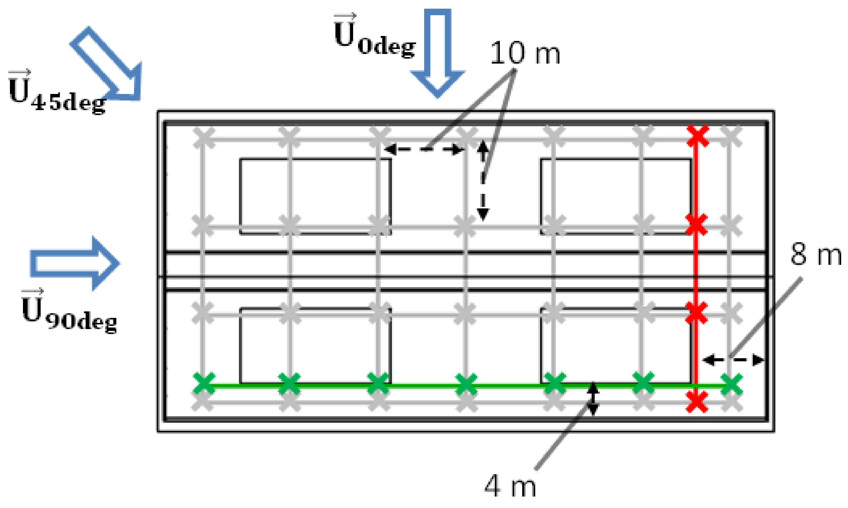
2.3.3. Boundary Conditions: Velocity, RiValues

The inlet velocity describes an atmospheric boundary layer (ABL) profile with the equation [6]:
U ( y ) = U r e f y y r e f α
Here, U ( y ) is the inlet velocity profile (in m s 1 ), U r e f is the chosen velocity (in m s 1 ) at height y r e f (in m), and α is a power coefficient (without dimension). The value of α = 0.16 was extracted from our wind tunnel measurements. y r e f was chosen as half of the AOZ height ( y r e f = H A O Z / 2 = 0.8 m). The roughness of 0.068 m, corresponding to a moderately rough terrain, was set at the ground in order to conserve the form of the ABL profile [12]. The domain boundary conditions were set in relation to the inflow air angle. Table 3 shows the details.
The Richardson number Ri (= Grashof number/Reynolds number 2 ) is the ratio of the buoyancy forces and the kinetic forces and is used to distinguish three types of convection. When Ri > 5, the buoyancy forces represented by the Grashof number Gr prevail over the kinetic forces represented by the Reynolds number Re. When 0.2 < Ri < 5, the buoyancy forces are on par with the kinetic forces. For Ri < 0.2, the kinetic forces are dominant [16]. Six values of the Richardson number were considered to cover the three types of convection and the different seasons of the year, recapitulated in Table 4.

2.3.4. Sampling Strategy for Gas Concentration Evaluation of the Study

For this numerical study, the gas concentration was evaluated at different points as described in Figure 6. Inside the barn, twenty-eight points forming a net (grey crosses) were designed with a distance of 10 m between the points respecting the measurement strategy for NVBs. Since this is a numerical CFD study, we chose the expression “evaluation points” instead of “measurement points” in order to emphasize the virtual character of the study. Evaluation points forming lines at the outcoming flow directions were set as well inside the barn. Those settlements of the points for the evaluation of the gas concentration were extracted from the work of [1].
The mixing gas concentration ratios M n e t = C N H 3 / C C O 2 n e t and M l i n e = C N H 3 / C C O 2 l i n e were evaluated as the mean concentration of NH 3 over the net (grey) points or over the lines (green and red) points divided by the mean concentration of CO 2 over the net or line points. The considered line points depended on the air inflow direction. For the airflow in the 0 deg direction, M l i n e = M g r e e n l i n e , only the mean concentrations over the points of the green line were considered. For the airflow in the 90 deg direction, M l i n e = M r e d l i n e , only the mean concentrations over the points of the red line were considered. For the airflow in the 45 deg direction, M l i n e = M g r e e n r e d l i n e s , we considered the mean concentrations over the points of both the green and red lines. Those ratios were compared with the source gas concentration M s o u r c e = C N H 3 / C C O 2 s o u r c e as a reference. Thus, we looked for the condition q u o t i e n t 1 to be verified.
q u o t i e n t 1 = ( M N H 3 / C O 2 ) n e t o r l i n e / ( M N H 3 / C O 2 ) s o u r c e = 1

3. Results and Discussion

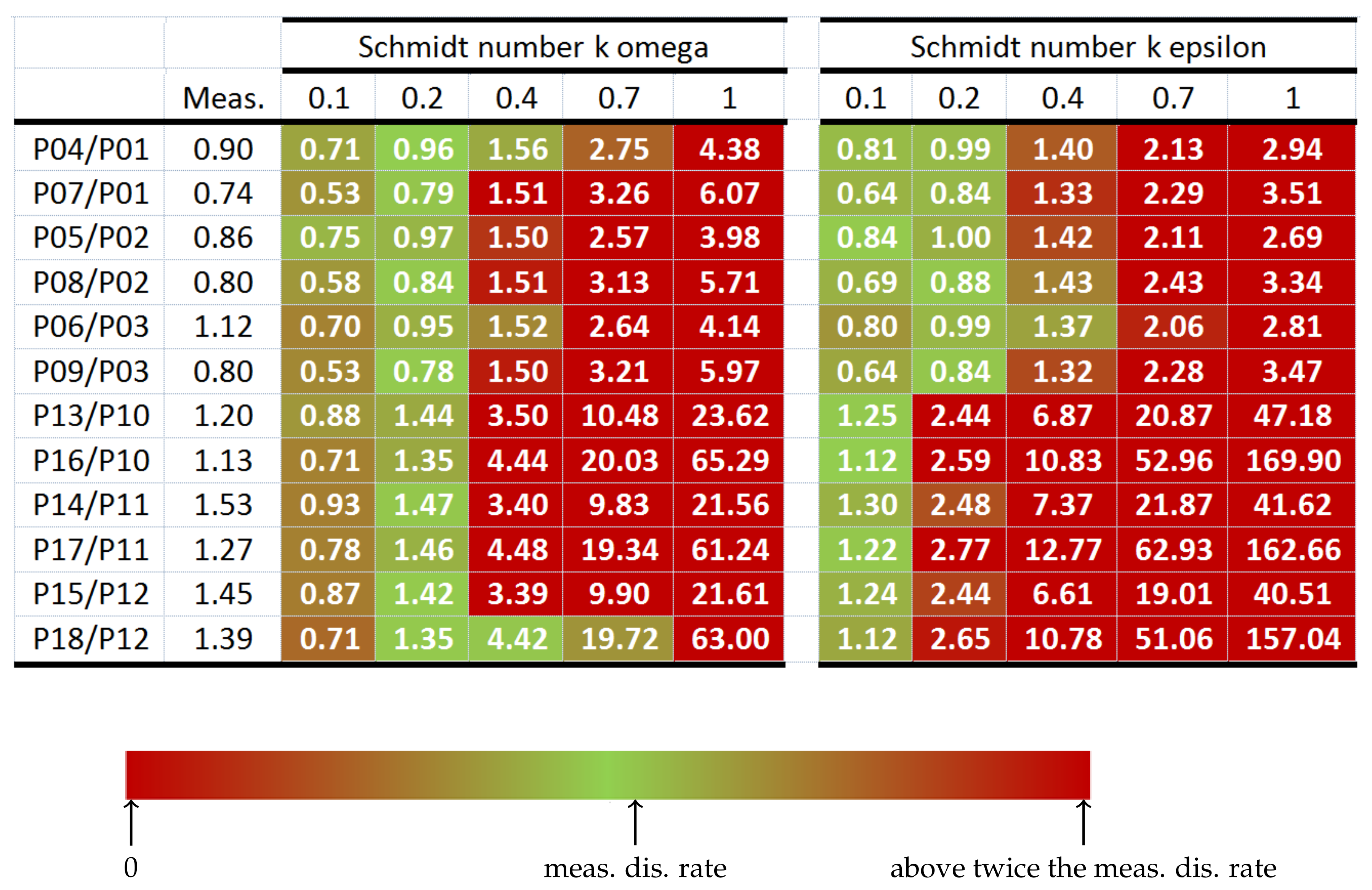
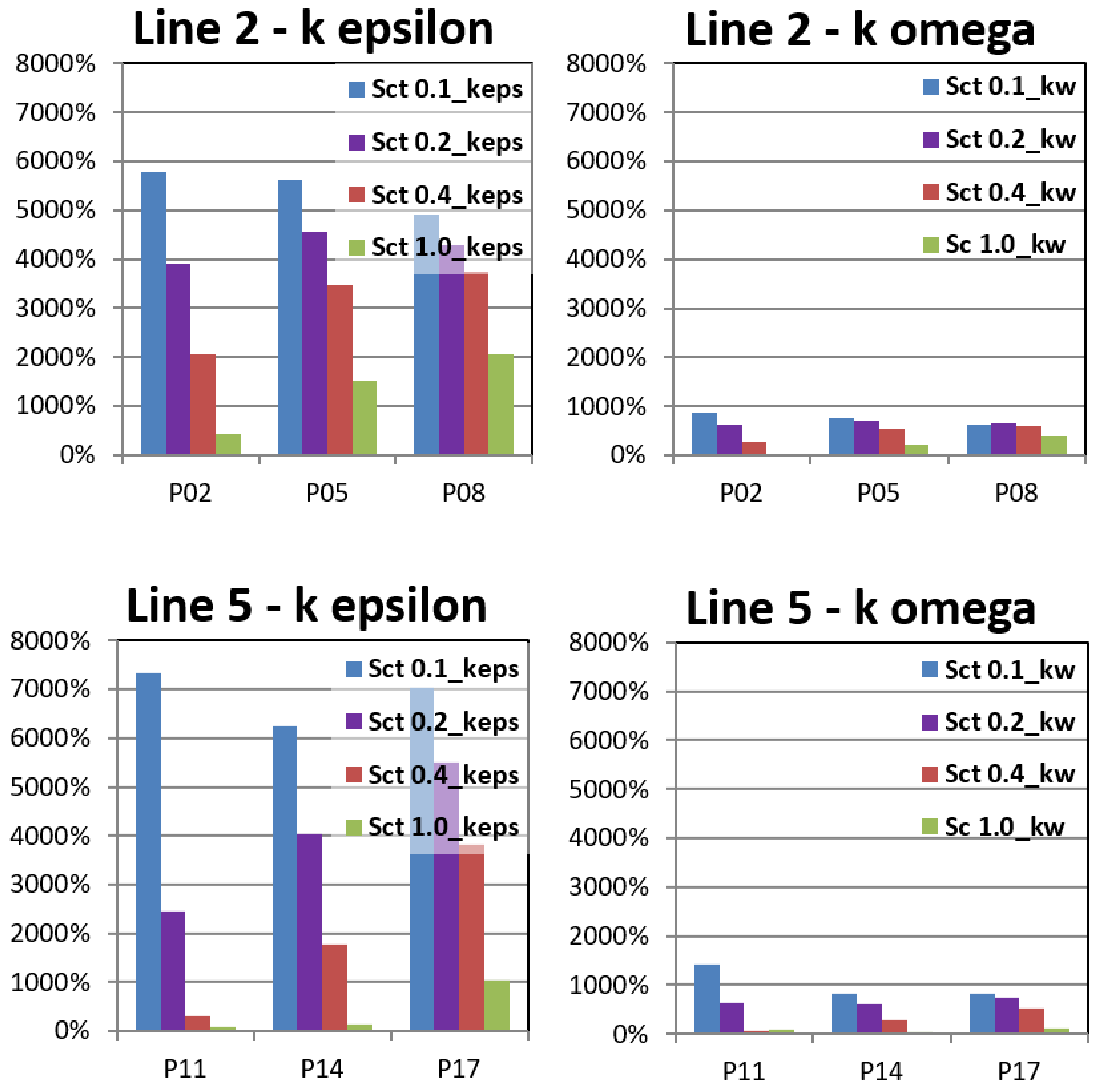
3.1. Influence of the Sct-Number

In Figure 7, the simulated dispersion rates are presented in term of tables filled with colors using the “colors scale” of the Microsoft Excel “conditional formatting” tool. For both tables (k omega and k epsilon), each row corresponds to the simulated dispersion rate for different Sct-numbers with, at the far left, the measured dispersion rate from the wind tunnel experiment (denoted “Meas.” and without color). Within each row, the simulated dispersion rates are compared with the measured dispersion rate, which serves as a reference (denoted “meas. dis. rate” in the color bar). The result of this comparison is color-coded. The greener the cell in the table is, the closer is the simulated value listed there to the associated measurement. The larger the deviation between the simulated dispersion rate and the measured dispersion rate is, the more red the cell becomes. The extreme values (i.e., color red) of the color bar are zero (minimum, as the dispersion rate cannot be negative) and at least twice the measured dispersion rate (for the maximum). The left table corresponds to the k-omega model, and the right table corresponds to the k-epsilon model.
Overall, it can be seen that the higher the Sct-number is, the higher is the dispersion rate, reaching the maximum value of about 65 for the k-omega model and about 170 for the k-epsilon model, both for a Sct-number equal to one. Considering the k-omega model result, the dispersion rates matching the measurement values best are those of the Sct-number equal to 0.2. In the case of the k-epsilon model, it is the Sct-number equal to 0.1 that has the most suitable dispersion rates.
We took another look at the results, but this time at the absolute gas concentration, in terms of percentage, from the numerical simulation relative to the measured concentration at each point i for comparison, see Equation (5). As representative examples, we chose to show, in Figure 8, the values at the points of the middle Lines 2 and 5 (see Figure 2). Overall, we noticed an overprediction of the absolute concentrations for both models, but the k-epsilon concentrations were 10 times higher than the ones from k-omega.
C ( i , s i m u l a t e d ) C ( i , m e a s u r e d ) / C ( i , m e a s u r e d ) · 100
The high sensitivity of the concentration relatively to the Sct-number can be noted, as this was already shown in numerous previous studies recalled in the Introduction of this paper [7]. Our results showed that the lower the Sct-number, the higher was the overestimation of the concentration. A higher Sct-number, which means lower diffusion in order to compensate for the overestimation, led to more accurate concentrations. Chao Lin et al. [17] came to the same conclusion when analyzing high-buoyancy gas dispersion with the RANS model. As another telling example, Tominage et al. [18] also found a high discrepancy (three to five times) between the RANS model and the measurement when modeling pollution dispersion in a street canyon.
On the one side, for the k-omega model, the concentrations for a Sct-number of 0.2 in violet (the value of the Sct-number matching at best the measured dispersion rate) were almost constant around 600–700%. On the other side, for the k-epsilon model, the concentrations for a Sct-number of 0.1 in blue (value matching at best the measured dispersion rate) varied greatly from one point to another from 4900–7300%.
Those results led us to the conclusion that the k-omega model with the Sct-number equal to 0.2 can be retained for the study. This was because with this setup, the dispersion rates had a good match with the measurements. Moreover, the simulated and measured absolute concentrations at all points had almost a constant difference, which permitted extracting a constant factor between the simulation and reality.

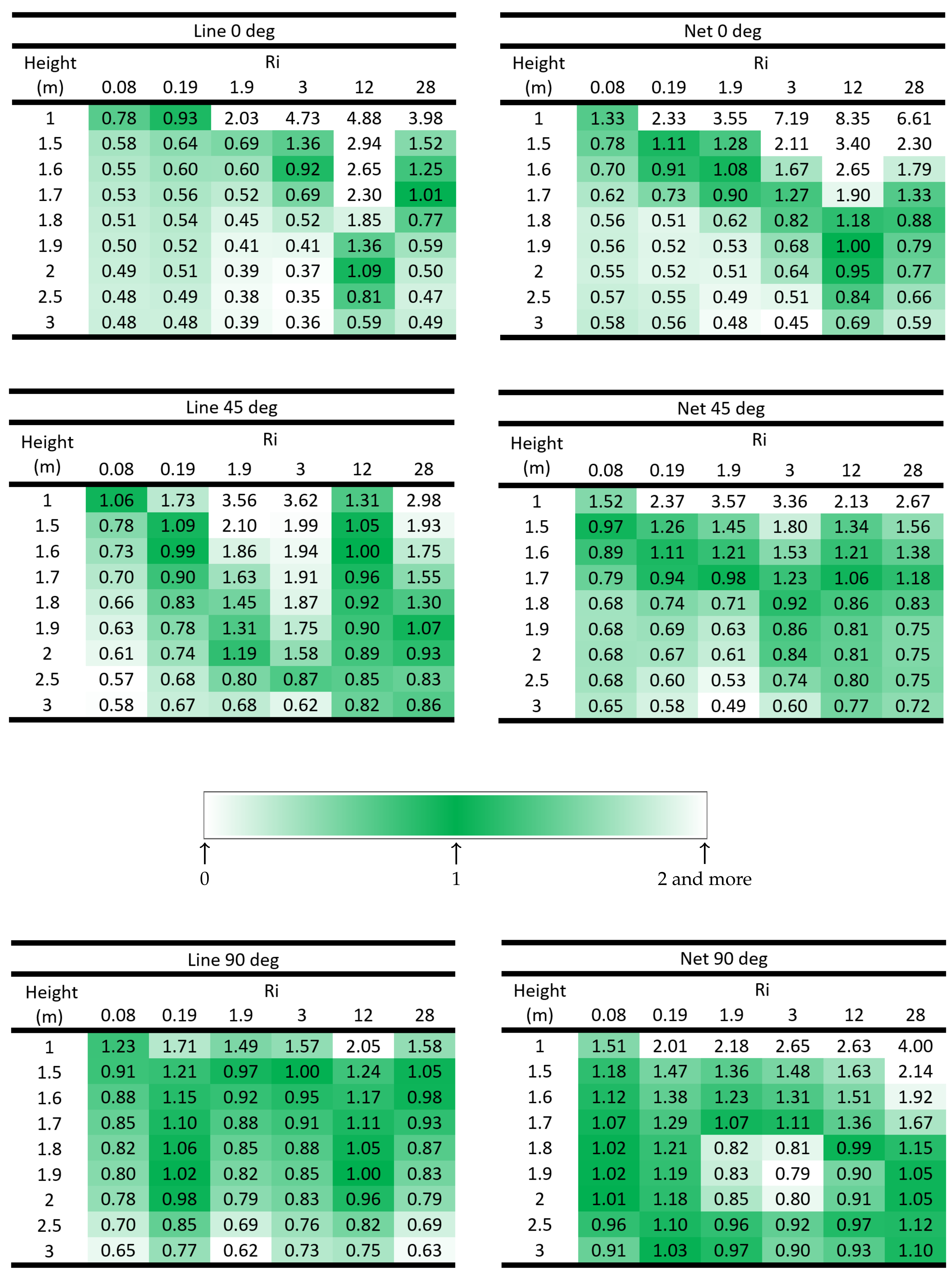
3.2. Mixing Gas Concentration at Different Heights

Figure 9 summarizes the quotient of the gas concentration mixing ratios evaluated at the net and line points described in Section 2.3 and the gas concentration mixing ratio from both the CO 2 and NH 3 sources. The results are presented for the three incoming air flow directions with six Ri values. Usually, the emission rates of the pollutant NH 3 were evaluated through Equation (6):
E N H 3 = c o n s t a n t · C N H 3 / C C O 2 s o u r c e
This supposes that the mean mixing ratio C N H 3 / C C O 2 is measured at the height and through a group of sampling points that represent the ratio C N H 3 / C C O 2 at the sources. Putting this into the equation, we looked for the following equality of Equation (4). Based on this knowledge and with the objective to facilitate the interpretation, we used again the “conditional formatting” tool of Microsoft Excel to color in green the table cells close to one and in white color the extreme values of zero and two and beyond. From the tables, it can be first noticed that for all cases, the height of the evaluation lines and net played an important role.
In general, the quotient of the mixing ratio became smaller with increasing height for all considered inflow directions and convection regimes. For 0 deg and 45 deg under mixed and forced convection conditions (Ri < 5), when the air velocity became more dominant (Ri tends to lower values), the representative height (the height respecting the condition q u o t i e n t 1 ) became lower. In particular, under the conditions of mixed convection, the quotients of the mixing ratios varied considerably over the different heights. Here, we observed differences in the quotients of the concentration ratio between 1 m and 3 m of 7.19 (Ri = 3 and Net 0 deg) as the maximum value and 0.36 as the minimum value (Ri = 3 and Line 0 deg). In contrast, for 0 deg and 45 deg and forced convection (Ri < 0.2), as well as for 90 deg with Ri < 5, the quotient of the mixing ratios between 1 m and 3 m varied by less than one. For all cases (the three inflow directions and all net and line evaluations), under the conditions of natural convection (Ri > 5), the representative height effect was greater than under mixed and forced convection (Ri < 5). Under mixed convection (0.2 < Ri < 5), a suitable height was typically around 1.8 m (but the most representative positions differed depending on the wind direction and the temperature gradient).
An experimental study by Mendes et al. [3] under the conditions of mixed and force convection and cross-flow concluded that gas samples should be taken above a 2 m height as the mixing ratios became rather stable above this height. Our numerical simulation results under similar boundary conditions reproduced this general behavior of the mixing ratios. However, our results highlighted that a constant mixing ratio with height did not necessarily coincide with the best reproduction of the initial gas release ratio. Moreover, our simulation results indicated that the optimum height depended on the convection flow regime. At present, a value of at least a 3 m height for gas measurements is recommended to minimize the effect of animals, cubicles, and other obstacles in the VERA test protocol [4], which gives a guideline on the measurement strategy for naturally ventilated buildings. In our parametric study, however, this height turned out to rarely correspond to a perfect mixing. In our simulations, the initial concentration ratio was in most cases considerably underestimated when measuring at a 3 m height (with quotients of concentration ratios between 0.36 and 0.97). Only two cases (i.e., net measurement with 90 deg inflow and Ri = 0.19, as well as Ri = 28) resulted in quotients of the concentration ratios slightly larger than one when measuring at a 3 m height. It can also be observed that for each case, there was a height corresponding to a value that was close to quotient 1 and that this height was a little higher for the net evaluation in comparison to the line evaluation for the same case (same Ri value and same inlet flow direction). This led to the conclusion that, when knowing the right height, designing the evaluation points as a line at the barn outlet flow was enough to fulfil the condition of mixing flows.

4. Conclusions

In this paper, a reasonable value of the Schmidt number corresponding to the application of gas dispersion in the atmospheric boundary was found as a value of 0.2 for the RANS k-omega turbulence model. This value was obtained by comparing the wind tunnel measurements against different RANS simulations with the Sct-number varying from 0.1 to one. The influence of the Sct-number on the gas dispersion shown in the literature was confirmed. The higher the Sct-number, the higher the dispersion rate was, but at the same time, the lower the gas concentration was.
From our subsequent parameter study, we concluded that for most of the flow conditions considered in our study, the height for the perfect mixing ratio was between 1.5 m and 2.5 m (in our setup, this measurement height corresponded to about 13% to 22% of the building height and 33% to 55% of the opening height). For the most common case of mixed convection, the predicted optimal measurement height was around 1.8 m. This led to two important deductions. First, the influence of the Richardson number and the inlet flow direction was important since even for the range of nearly perfect mixing (1.5–2.5 m), the quotient of the NH 3 /CO 2 mixing ratio could vary from 0.35 to 3.40. Second, very few convection cases corresponded to the current common recommendation of at least a 3 m measurement height for a perfect mixing ratio.
Another important finding is that with the sampling line placed at the outgoing flow direction of the barn, the perfect mixing condition could be fulfilled (at the right height) with comparable accuracy as with a whole net of sampling points. This means that the commonly recommended line measurements are in principle reasonable. Other solutions of on-farm measurement strategies can be tested; for example, a vertical net of sampling points at the outgoing flow direction of the barn with grid points of 0.1 m × 10 m (height × length) might be considered to further increase the measurement accuracy with tracer gas methods. Further investigations will be needed in order to deepen our understanding of the mixing gas in NVBs. In the present study, the considered barn had a fixed width/length ratio and openings without curtains. The influence of the building and opening designs on the gas mixing ratio at different evaluation heights should be considered in future studies.

Author Contributions

Conceptualization, E.M.D., D.J., Q.Y., and Sabrina Hempel; methodology, E.M.D., D.J., Q.Y., and S.H.; software, E.M.D.; validation, E.M.D.; formal analysis, E.M.D., D.J., Q.Y., and S.H.; investigation, E.M.D.; writing—original draft preparation, E.M.D.; writing—review and editing, D.J., Q.Y., G.Z., T.A., M.K., and S.H.; visualization, E.M.D.; supervision, T.A., M.K., and S.H.; project administration, S.H.; funding acquisition, S.H. and D.J. All authors read and agreed to the published version of the manuscript.

Funding

The research was funded by the Deutsche Forschungsgemeinschaft (DFG, German Research Foundation), Grant Number 397548689. We further thank Sai Krishna Danda for his support in typesetting the paper.

Institutional Review Board Statement

Not applicable.

Informed Consent Statement

Not applicable.

Conflicts of Interest

The authors declare no conflict of interest.

Abbreviations

The following abbreviations are used in this manuscript:
CFDComputational fluid dynamics
NVBNaturally ventilated barns
RANSReynolds-averaged Navier–Stokes
ABLWTAtmospheric boundary layer wind tunnel
AOZAnimal-occupied zones

References

  1. Janke, D.; Willink, D.; Ammon, C.; Hempel, S.; Schrade, S.; Demeyer, P.; Hartung, E.; Amon, B.; Ogink, N.; Amon, T. Calculation of ventilation rates and ammonia emissions: Comparison of sampling strategies for a naturally ventilated dairy barn. Biosyst. Eng. 2020, 198, 15–30. [Google Scholar] [CrossRef]
  2. Saha, C.; Fiedler, M.; Ammon, C.; Berg, W.; Loebsin, C.; Amon, B.; Amon, T. Uncertainty in calculating air exchange rate of naturally ventilated dairy building based on point concentrations. Environ. Eng. Manag. J. 2014, 13, 2349–2355. [Google Scholar] [CrossRef]
  3. Mendes, L.B.; Edouard, N.; Ogink, N.W.; van Dooren, H.J.C.; de Fátima, F.; Tinôco, I.; Mosquera, J. Spatial variability of mixing ratios of ammonia and tracer gases in a naturally ventilated dairy cow barn. Biosyst. Eng. 2015, 129, 360–369. [Google Scholar] [CrossRef]
  4. VERA. VERA Test Protocol for Livestock Housing and Management Systems; Technical Report; European Union: Brussels, Belgium, 2018. [Google Scholar]
  5. Drewry, J.L.; Choi, C.Y.; Powell, J.M.; Luck, B.D. Computational model of methane and ammonia emissions from dairy barns: Development and validation. Comput. Electron. Agric. 2018, 149, 80–89. [Google Scholar] [CrossRef]
  6. Blocken, B. LES over RANS in building simulation for outdoor and indoor applications: A foregone conclusion? Build. Simul. 2018, 11, 1–50. [Google Scholar] [CrossRef] [Green Version]
  7. Gualtieri, C.; Angeloudis, A.; Bombardelli, F.; Jha, S.; Stoesser, T. On the Values for the Turbulent Schmidt Number in Environmental Flows. Fluids 2017, 2, 17. [Google Scholar] [CrossRef] [Green Version]
  8. Gromke, C.; Buccolieri, R.; Di Sabatino, S.; Ruck, B. Dispersion study in a street canyon with tree planting by means of wind tunnel and numerical investigations—Evaluation of CFD data with experimental data. Atmos. Environ. 2008, 42, 8640–8650. [Google Scholar] [CrossRef]
  9. Gorlé, C.; Beeck, J.; Rambaud, P. Dispersion in the Wake of a Rectangular Building: Validation of Two Reynolds-Averaged Navier–Stokes Modelling Approaches. Bound. Layer Meteorol. 2010, 137, 115–133. [Google Scholar] [CrossRef]
  10. Janke, D.; Yi, Q.; Thormann, L.; Hempel, S.; Amon, B.; Nosek, Š.; van Overbeke, P.; Amon, T. Direct Measurements of the Volume Flow Rate and Emissions in a Large Naturally Ventilated Building. Sensors 2020, 20, 6223. [Google Scholar] [CrossRef] [PubMed]
  11. Lanfrit, M. Best Practice Guidelines for Handling Automotive External Aerodynamics with FLUENT; Fluent Deutschland GmbH: Darmstadt, Germany, 2005. [Google Scholar]
  12. Doumbia, M.; Hempel, S.; Janke, D.; Amon, T. Prediction of the Local Air Exchange Rate in Animal Occupied Zones of a Naturally Ventilated Barn. In Proceedings of the XXXVIII CIOSTA & CIGR V; XXXVIII CIOSTA & CIGR V International Conference, Rhodes Island, Greece, 24–26 June 2019; pp. 29–34. [Google Scholar]
  13. Doumbia, E.M.; Janke, D.; Yi, Q.; Amon, T.; Kriegel, M.; Hempel, S. CFD modelling of an animal occupied zone using an anisotropic porous medium model with velocity depended resistance parameters. Comput. Electron. Agric. 2021, 181, 105950. [Google Scholar] [CrossRef]
  14. Van Hooff, T.; Blocken, B.; Gousseau, P.; van Heijst, G. Counter-gradient diffusion in a slot-ventilated enclosure assessed by LES and RANS. Comput. Fluids 2014, 96, 63–75. [Google Scholar] [CrossRef]
  15. Pedersen, S.; Sällvik, K. 4th Report of Working Group on Climatization of Animal Houses Heat and Moisture Production at Animal and House Levels; Technical Report; Research Centre Bygholm: Horsens, Denmark, 2002; p. 343. [Google Scholar]
  16. Marek, R.; Nitsche, K. Praxis der Wärmeübertragung Grundlagen—Anwendungen—Übungsaufgaben; 4., Neu Bearbeitete Auflage; Carl Hanser Verlag GmbH & Co. KG: Deggendorf, Germany, 2015. [Google Scholar]
  17. Lin, C.; Ooka, R.; Kikumoto, H.; Sato, T.; Arai, M. CFD simulations on high-buoyancy gas dispersion in the wake of an isolated cubic building using steady RANS model and LES. Build. Environ. 2020, 188, 107478. [Google Scholar] [CrossRef]
  18. Tominaga, Y.; Stathopoulos, T. CFD modeling of pollution dispersion in a street canyon: Comparison between LES and RANS. J. Wind Eng. Ind. Aerodyn. 2011, 99, 340–348. [Google Scholar] [CrossRef] [Green Version]
Figure 1. Wind tunnel description; in our setup, the model is the porous stone material described in Section 2.1.2.
Applsci 11 04560 g001
Figure 2. Measurement setup; the pictures are non-dimensional; here, w = 342 mm and h = 15 mm.
Applsci 11 04560 g002
Figure 3. (a) Domain dimensions and boundary conditions with L (=255 mm) as the length of the porous stone; (b) view of the mesh.
Applsci 11 04560 g003
Figure 4. (a) Description of the domain dimensions and the three inlet flow directions; (b) focus on the barn dimensions and the AOZs (red), CO 2 sources (blue), and NH 3 sources (green).
Applsci 11 04560 g004
Figure 5. Description of the principle of the cows’ (left) replacement by porous medium (right) in terms of the pressure drop and heat transfer. The velocity contour evaluated in the horizontal plane of height H A O Z /2.
Applsci 11 04560 g005
Figure 6. Design of the net and lines of points for the concentration evaluations.
Applsci 11 04560 g006
Figure 7. Comparison between the measured and simulated dispersion rate.
Applsci 11 04560 g007
Figure 8. The influence of the turbulent Schmidt number on the simulated absolute concentration of gas relative to the measured concentration; evaluation at the points of Lines 2 and 5; left, the result of the k-epsilon model, and right, the result of the k-omega model.
Applsci 11 04560 g008
Figure 9. Quotient of mixing ratios of the gas concentrations ( ( M N H 3 / C O 2 ) n e t / l i n e )/( ( M N H 3 / C O 2 ) s o u r c e ) with the lines and net at different heights, for diverse values of the Richardson numbers and for the 3 incoming flow directions.
Applsci 11 04560 g009
Table 1. Gas concentration evaluation points and corresponding lines.
LinesPoints
Line 1P01; P04; P07
Line 2P02; P05; P08
Line 3P03; P06; P09
Line 4P10; P13; P16
Line 5P11; P14; P17
Line 6P12; P15; P18
Table 2. Grid convergence.
Domain Cell NumberAll Points’ Mean Concentration Rel. Diff. in %
1,158,870
2,728,87826.6%
3,319,1025.8%
Table 3. Boundary conditions corresponding to the flow directions.
Inflow DirectionNorth SideSouth SideWest SideEast Side
0 degvelocity inletpressure outletwallwall
45 degvelocity inletpressure outletvelocity inletpressure outlet
90 degWallwallvelocity inletpressure outlet
Table 4. Detailed Ri values and corresponding velocities and temperatures.
Ri Cases
Ri < 0.20.2 < Ri < 5Ri > 5
Ri = 0.078Ri = 0.198Ri = 1.9Ri = 3.0Ri = 12.0Ri = 28.0
T a i r (°C)3022151070
U r e f (m s 1 )2.82.50.970.850.450.33
SeasonSummerFall-SpringWinter
Publisher’s Note: MDPI stays neutral with regard to jurisdictional claims in published maps and institutional affiliations.

