Distortion of Thomson Parabolic-Like Proton Patterns Due to Electromagnetic Interference

Abstract

Intense electromagnetic pulses (EMPs) accompany the production of plasma when a high-intensity laser irradiates a solid target. The EMP occurs both during and long after the end of the laser pulse (up to hundreds of nanoseconds) within and outside the interaction chamber, and interferes with nearby electronics, which may lead to the disruption or malfunction of plasma diagnostic devices. This contribution reports a correlation between the frequency spectrum of the EMP and the distortion of Thomson parabola tracks of protons observed at the kJ-class PALS laser facility in Prague. EMP emission was recorded using a simple flat antenna. Ions accelerated from the front side of the target were simultaneously detected by a Thomson parabola ion spectrometer. The comparison of the two signals suggests that the EMP may be considered to be the source of parabolic track distortion.

1. Introduction

A traditional Thomson parabola ion spectrometer (TP) is a device that can distinguish ions propagating through it according to their charge-to-mass ratio and their kinetic energy [1]. The spectrometer employs parallel magnetic and electric fields that are perpendicularly arranged with respect to the ion propagation direction. Particles entering a pinhole in the front are deflected and they then interact with an image plane where a recording system is installed (e.g., plastic nuclear track detector, photostimulable image plate, or microchannel plate coupled to a phosphor screen and a charge-coupled device camera). Typically, the magnetic field is provided by two parallel magnets, and the electric field is created by applying a voltage to electrical plates through high-voltage cables. Theoretically, perfect parabolic tracks of ions are drawn in the spectrometer detector plane. Nevertheless, the tracks can be perturbed by a high-energy laser pulse under real experimental conditions.

A major source of ion-track distortions is EMP, which is generated during laser–target interaction [2,3,4]. High-voltage cables connected to the TP can pick up EMP noise during a laser shot, which results in the distortion of the spectrometer electric field. Ions with different energies thus experience varying electric-field strength, and their tracks on the detector plane are distorted. The high-pass filter on high-voltage cables can be incorporated in order to reduce this effect [5]. Alternatively, Faraday cage shielding around cables and the spectrometer can be used to mitigate this effect.

Another source of deviation from perfect tracks is attributed to the emission direction of the laser-accelerated proton beam itself at the the target surface (which is usually called “pointing”). A high-spatial-resolution Thomson spectrometer was employed to measure the pointing of proton beams generated from the rear side of plane target foils. Small bumps and deviations from the perfect parabolic tracks of ions were observed and identified as a feature of the emitted proton beam that occurred due to small fluctuations in the acceleration sheath [6].

Track oscillations and distortions complicate the analysis and interpretation of ion numbers, especially when many different kinds of ion species are detected by the spectrometer. The overlapping of proton tracks and fast ion tracks can appear (as demonstrated in Figure 1) and lead to an incorrect number of detected particles. In addition, fitting and extracting the parabolic trajectories becomes difficult, as they do not follow smooth analytically derived curves. Here, we report the observation of distorted parabolic tracks at the PALS laser facility when a 600 J, 350 ps (FWHM) laser pulse was focused on solid targets reaching an intensity of $3\times {10}^{16}$ W/cm${}^2$. Since the EMP affecting plasma diagnostics can be effectively detected by a simple antenna, and the recorded signal can be processed in the frequency domain [7,8], we compared the measured EMP signal with distorted parabolic tracks in order to investigate the effect of the EMP on the spectrometer, and to prove that the cause of track distortions at the PALS laser facility is the strong EMP generated in the target chamber.

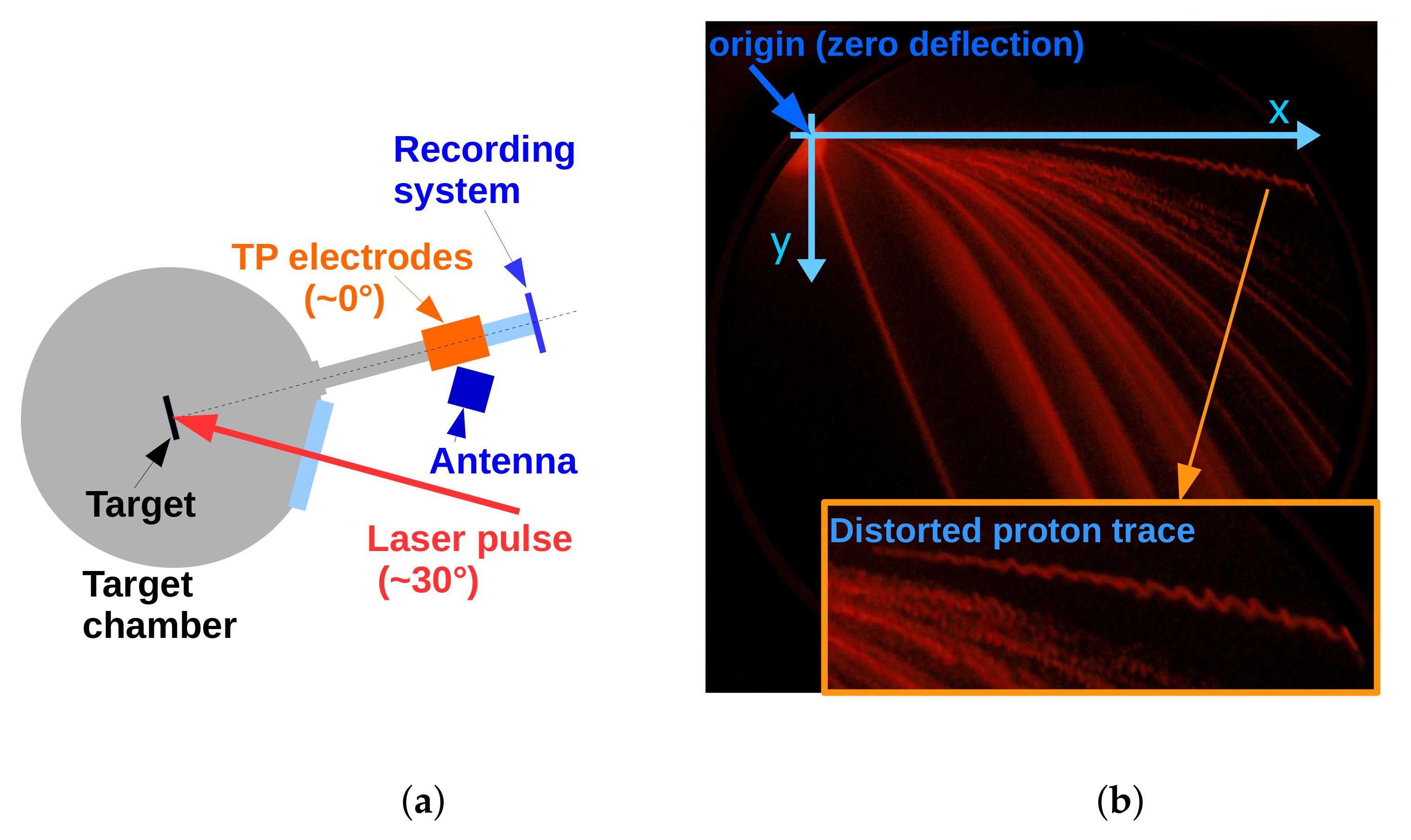
2. Experimental Arrangement and Measurement

A 2 TW iodine laser system with a wavelength of 1315 nm was employed to irradiate targets composed of polymethyl methacrylate or silicon wafers doped with boron. The ions accelerated in the backward direction were detected by the TP placed at a $0^{\circ }$ detection angle with respect to the normal target surface and at a distance of 2.17 m from the target (see Figure 2).

The spectrometer used a microchannel plate coupled to a phosphor screen and to the CCD. The strength of the TP’s magnetic field was increased up to 0.12 T. A potential difference of 2.9 kV was applied across the 21.5 mm wide gap between the spectrometer electrical plates in order to reach a separation of the ion tracks on the spectrometer’s detection system. The parabolic tracks on the image plane (within Cartesian coordinate system $(x,y)$ and under nonrelativistic approximation) are described by the following Equation [9]:

$$y=\frac{q}{m_0}\frac{E{L}_{fE}\left(\frac{L_{fE}}{2}+L_{rE}\right)}{B{L}_{fB}\left(\frac{L_{fB}}{2}+L_{rB}\right)}{x}^2,$$

(1)

where q is the charge of ion, $m_0$ is its invariant mass, E is the strength of the spectrometer’s electric field, B is the strength of its magnetic field, $L_{fE}$ ($L_{fB}$) is the length of the electric (magnetic) field, and $L_{rE}$ ($L_{rB}$) stands for the distance between the end of the electric (magnetic) field and the recording system, respectively. The x axis was oriented in the direction of ions deflection in the magnetic field, and the y axis was oriented in the direction of their deflection in the electric field.

Figure 2 also shows a typical TP snapshot with the Cartesian coordinate system, where the parabolic track corresponding to protons is distorted due to EMP interference. While the protons were detected by the TP, the EMP generated in the target chamber and propagated outside from it was simultaneously recorded by a plane antenna positioned directly on the TP electrodes, as can be seen in Figure 2.

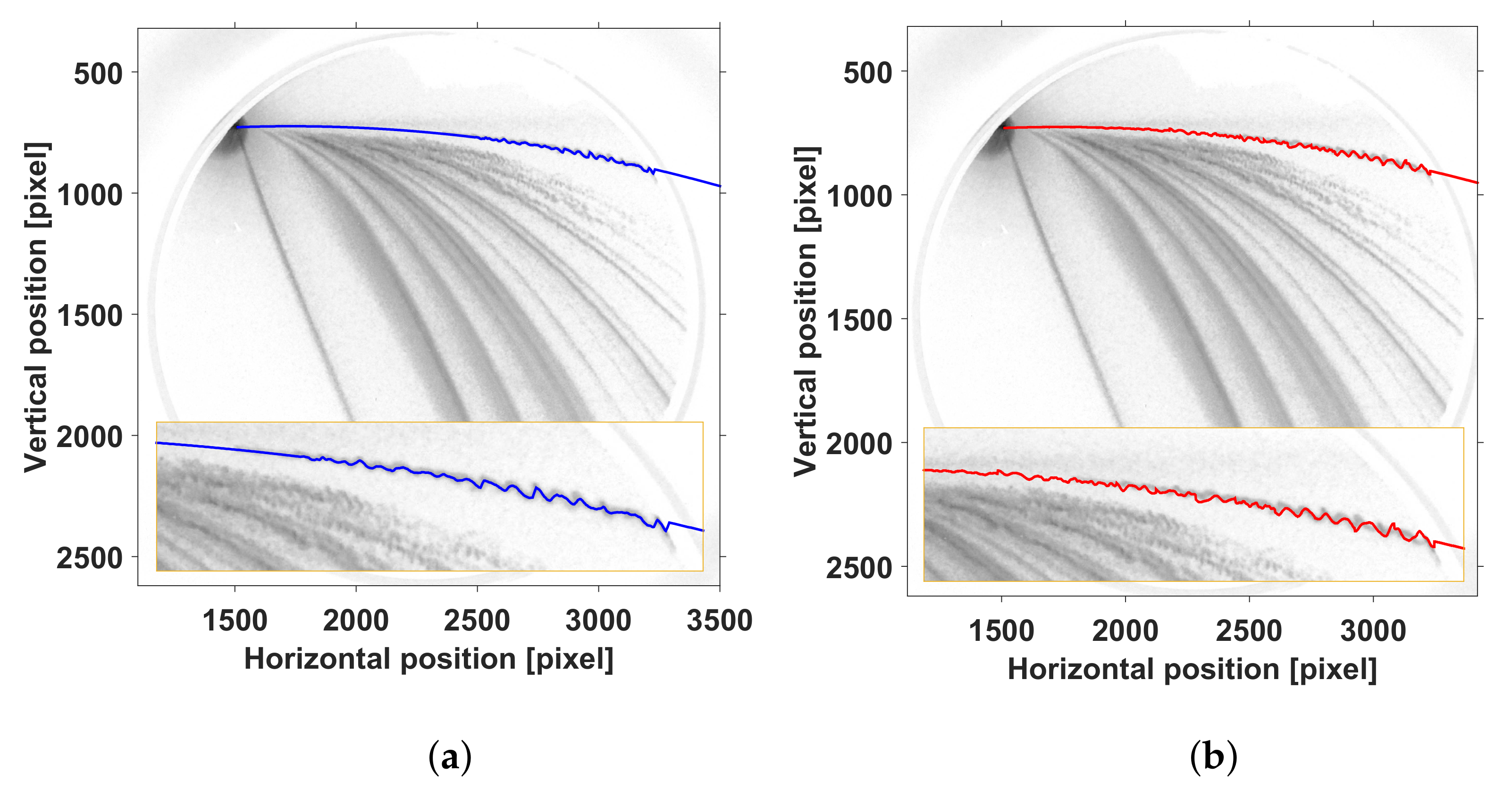
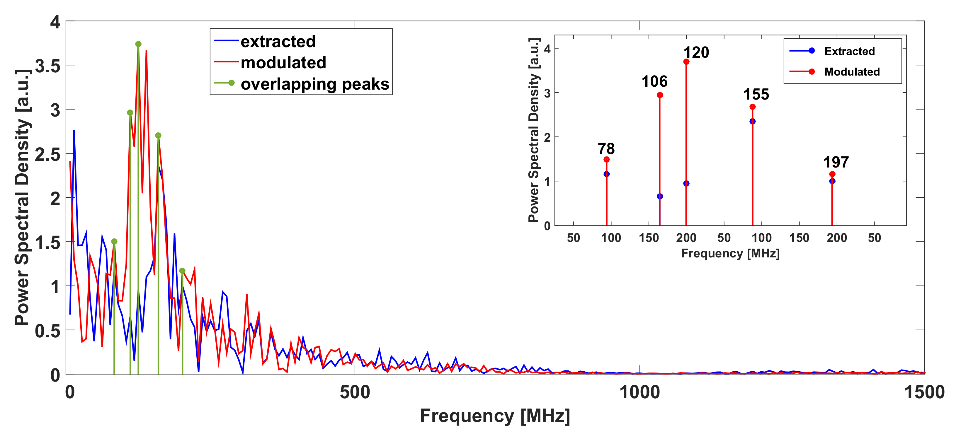
3. Processing Antenna Signals and TP Snapshots

The obtained data by both the TP and the antenna were processed by a MATLAB script specifically written for this purpose. First, the parabolic curve (1) that overlapped the track of protons was plotted in the TP snapshot. In such a way, one can read the intensity of pixels associated with the parabolic curve, and plot this intensity as a function of the horizontal position x with respect to the origin of the parabola (i.e., to the zero-deflection point). Then, the velocity of ions v was derived for every point of the parabola (i.e., for each pixel) from the general equation for magnetic deflection [9]:

$$v=\frac{qB{L}_{fB}}{x{m}_0}\left(\frac{L_{fB}}{2}+L_{rB}\right),$$

(2)

where x stands for the distance between the origin of the parabolic track and the actual position of an ion in the detector plane due to its deflection in the magnetic field. By knowing the distance between target and recording system, the corresponding proton time of flight (TOF) was calculated. Therefore, the dependence of the pixel intensity (along the parabolic curve) on the TOF of protons was derived for each point of the parabolic track as can be seen in Figure 3. This calculation shows which part of the EMP signal influenced the TP, because the antenna (recording the EMP signal) was positioned directly on the TP electrodes. As Figure 3 shows, the signal recorded by the antenna between 0 and 243 ns (the edge of the detector) corresponds to the entire parabolic track of protons from zero-deflection point up to the edge of MCP. Since the proton signal occurred only between 120 and 243 ns in this particular measurement, only the part of the EMP signal between 120 and 243 ns was considered in further processing. This part of the signal is highlighted with red in Figure 4, showing the measured antenna signal. The EMP that affected the TP before the fastest protons (in our case, before 120 ns) can also be included in analysis. This would basically also predict the distortion of the parabolic track in the region where no protons were detected in this experiment. Nevertheless, analysis was mainly focused on the region between 120 and 243 ns because the results could be compared with the measured parabolic track of protons.

The red part of the recorded EMP signal (i.e., the part corresponding to detected protons) in Figure 4 was divided into 9 samples. The length of each sample must be sufficient to retrieve its frequency spectrum using fast Fourier transform (FFT). This condition together with the length of the red part naturally led to the number of samples (in this case, N = 9). After applying the FFT on each time sample, we found 3 highest peaks corresponding to the 3 main frequencies $f_i^1,f_i^2,f_i^3$ included within the i-th time sample. In addition, phases ${\varphi }_i^1,{\varphi }_i^2,{\varphi }_i^3$ and amplitudes $A_i^1,A_i^2,A_i^3$ were obtained. Lastly, this physical quantities (frequencies, phases, and amplitudes) were used to calculate the modulated electric field $E_m$ in the model developed in MATLAB. In addition, frequencies $f_i^1,f_i^2,f_i^3$, which were found in time sample $t_i$, contributed to the modulation of the electric field only within time sample $t_i$, and their contribution was cancelled by setting $t_i=0$ outside this particular time sample. In such a way, the track of protons in time sample $t_i$ was distorted only by the electromagnetic waves that affected the TP while these protons were traversing the electric field. The other bunch of protons (e.g., related to time sample $t_{i+1}$) were influenced by waves that were interacting with the TP within time sample $t_{i+1}$. The modulation of electric field $E_m$ can be thus expressed as a function of time corresponding to the TOF of protons. The modulation itself is considered to be a sum of sine waves because the sources of modulations are electromagnetic waves generated during laser–target interaction. Assuming the linear transfer of modulation from EMP to electric field, sinusoidal modulations with main frequencies (and corresponding phases and amplitudes) were added to the constant term of the electric field. The relation for final electric field $E\left(t\right)$ in the model may be written as

$$E\left(t\right)=E_o+K·E_m(t,f_{i=1,\cdots ,9}^{j=1,\cdots ,3},{\phi }_{i=1,\cdots ,9}^{j=1,\cdots ,3})=E_o+K·\sum _{i=1}^9\sum _{j=1}^3{A}_i^j·sin(2\pi f_i^j{t}_i+{\phi }_i^j),$$

(3)

where $E_0$ is the electric field applied to the electrodes, and K is the constant that may be changed in order to amplify the influence of modulation. This constant was less important, since we only investigated the similarities of the frequency. Resulting electric field $E\left(t\right)$ was no longer constant and led to the distortion of parabolic tracks on the recording system. In particular, the electric field (3) was substituted in Equation (1), which is plotted in the TP snapshot. Additionally, the captured track of protons was extracted from the snapshot by finding the maximum of intensity in a neighborhood of the parabolic track of protons. Eventually, both the extracted parabolic and the modulate track could be plotted. Both curves are shown in Figure 5 with the TP snapshot converted into grayscale in the Cartesian coordinate system.

We now demonstrate that the signal detected by the antenna was the same as the one that influenced the TP electrodes. The generated EMP on the target could propagate through the vacuum pipe connecting the TP spectrometer to the interaction chamber. Therefore, the cutoff frequency of the waveguide with a circular cross-section (radius of 50 mm) was analytically derived in order to understand whether the EMP could affect the TP electrodes from the inside. The cutoff frequency of the TE${}_{11}$ mode (the fundamental transverse electric mode of circular waveguide) was calculated as ≈1.75 GHz, which means that any electromagnetic wave of lower frequency could not propagate through the vacuum pipe towards the spectrometer. Thanks to the EMP characterization already performed at PALS, the main portion of the EMP frequency spectrum could be found below 1.5 GHz [7,10]. Hence, the antenna placed on TP electrodes recorded the EMP causing the distortion of parabolic tracks.

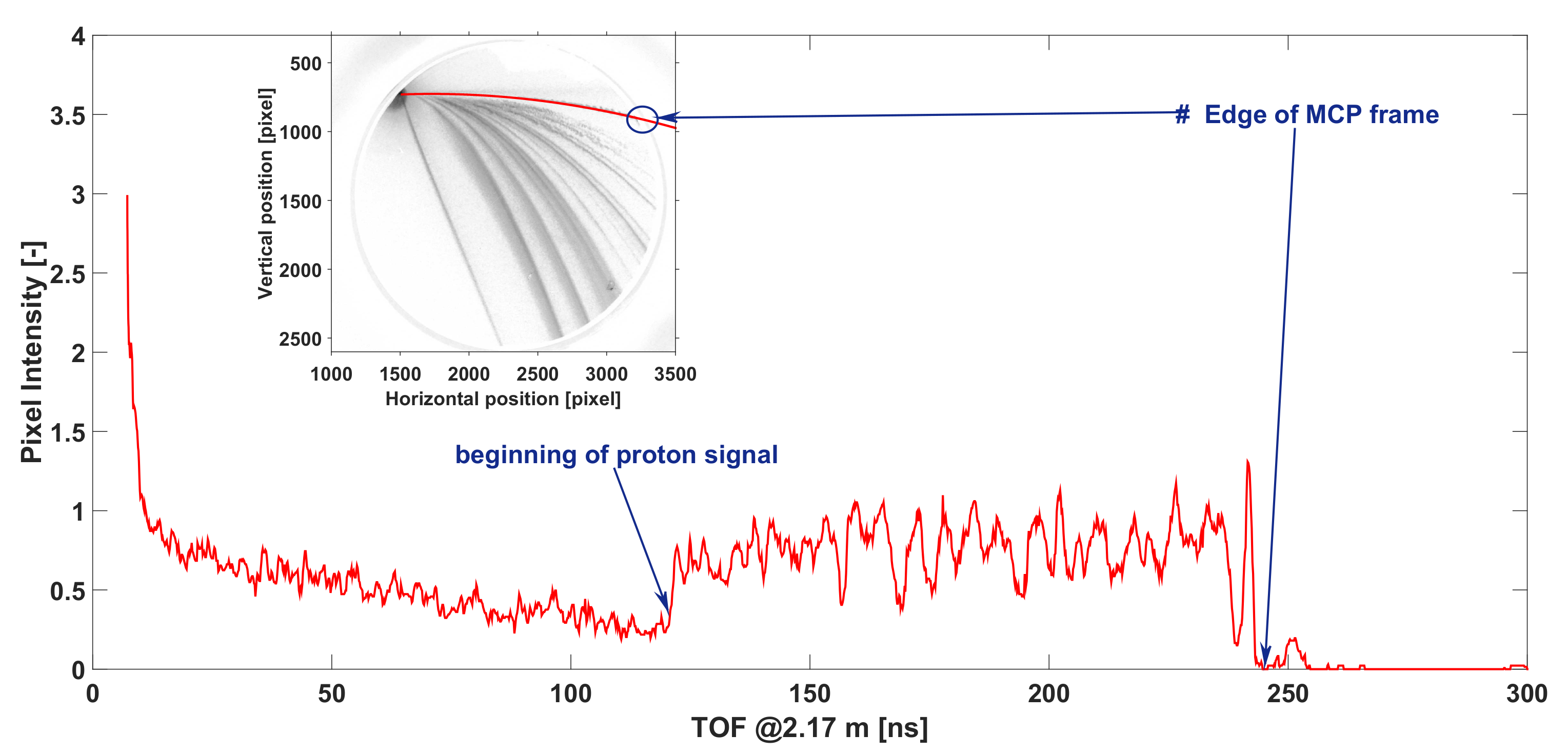
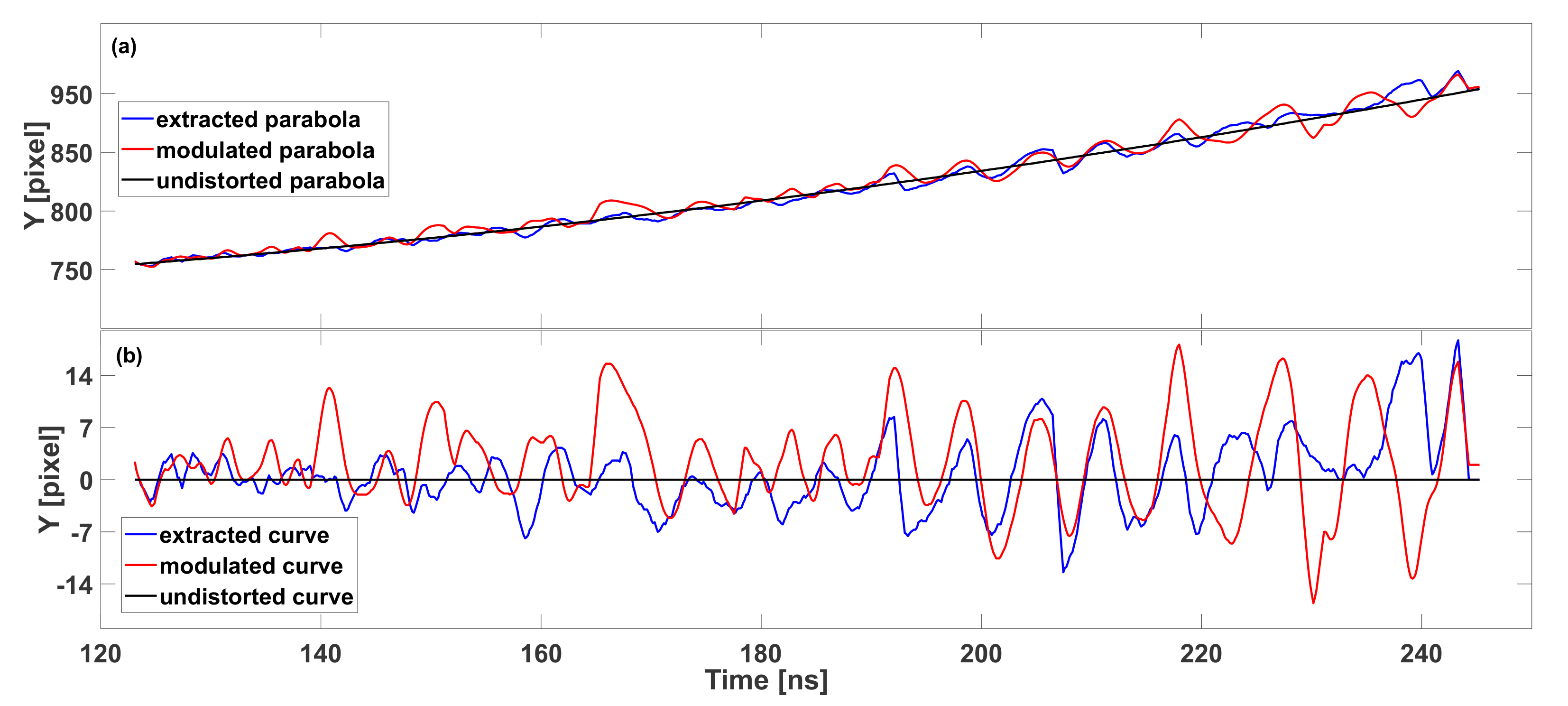
4. Correlation between Measured EMP and Captured Parabolic Track of Protons

In order to compare the extracted curve (blue) with the modulated one (red) in the time domain, we plotted both the extracted and the modulated parabolas as a function of TOF, as Figure 6 shows. In addition, the undistorted parabolic track is shown.

This curve corresponded to the ideal parabolic track that would be plotted in the image plane if the electric field were constant. Moreover, both curves in the frequency domain could be compared. Therefore, the parabolic dependence (1) was subtracted from all curves. Figure 6 shows both curves plotted as a function of TOF. Obviously, the undistorted parabola became a constant function without any variations due to the EMP. The modulation periods of both parabolas presented similarities. In order to quantify the similarity of the two curves in Figure 6, their frequency spectra were calculated and compared to each other. As it can be observed in Figure 7, the frequency ranges are almost identical. Additionally, we found the five highest peaks occurring at the same frequencies in both spectra. The result of this procedure is shown in the inset where the frequencies at which the peaks occur are listed. Since we are interested mainly in the values of frequencies on the x axis, the y axis of both plots were normalized. Consequently, both spectra in Figure 7 were integrated using the trapezoidal rule for approximating the definite integral and the ratio of integrals was calculated to be 1.2.

Similar correlation was observed by also analyzing several additional TP snapshots and the corresponding antenna signals. The ratios between the integrals of the extracted and modulated curves were estimated to vary between 0.7 and 1.3.

5. Conclusions

Distortions of parabolic ion tracks in a TP spectrometer were reported in the literature [5,6]. Unstable ion trajectories resulting into wiggles in the detector plane were assigned to the variation of the spectrometer’s electric field due to the EMP or to the pointing of the laser-accelerated proton beam itself.

On the basis of these observations, we carried out a series of measurements that showed correlation between the frequency spectrum of the EMP and the distortion of the parabolic-like tracks of protons on the recording system of the TP ion spectrometer at the PALS laser facility. In particular, frequencies extracted from the measured EMP signal were used to estimate the modulation of the electric field in our model. The parabolic tracks of protons obtained by Equation (3) and the measured ones presented similarities both in the time and the frequency domain. Frequency analysis of both the modulated and the measured parabolic curves showed that the frequency spectra had similar profiles, with peaks occurring at the same frequencies. Particularly, modulation frequencies between 50 and 200 MHz were found. In addition, the integrals of the frequency spectrum corresponding to both the modulated and the recorded parabola (i.e., the energy carried by the electrical signals) were alike. The ratios of such signal energies showed values in the range of 0.7–1.3. These observations led to the conclusion that the distortion of the spectrometer tracks detected at the PALS laser facility is caused by the EMP generated during and immediately after the high-energy laser–target interaction.

References

1. Olsen, J.N.; Kuswa, G.W.; Jones, E.D. Ion-expansion energy spectra correlated to laser plasma parameters. J. Appl. Phys. 1973, 44, 2275–2283. [Google Scholar] [CrossRef]
2. Brown, C.G.; Ayers, J.; Felker, B.; Ferguson, W.; Holder, J.P.; Nagel, S.R.; Piston, K.W.; Simanovskaia, N.; Throop, A.L.; Chung, M.; et al. Assessment and mitigation of diagnostic-generated electromagnetic interference at the National Ignition Facility. Rev. Sci. Instruments 2012, 83. [Google Scholar] [CrossRef] [PubMed] [Green Version]
3. Dubois, J.L.; Lubrano-Lavaderci, F.; Raffestin, D.; Ribolzi, J.; Gazave, J.; Fontaine, A.C.L.; D’Humières, E.; Hulin, S.; Nicolaï, P.; Poyé, A.; et al. Target charging in short-pulse-laser-plasma experiments. Phys. Rev. E Stat. Nonlinear Soft Matter Phys. 2014, 89. [Google Scholar] [CrossRef] [PubMed] [Green Version]
4. Consoli, F.; Tikhonchuk, V.T.; Bardon, M.; Bradford, P.; Carroll, D.C.; Cikhardt, J.; Cipriani, M.; Clarke, R.J.; Cowan, T.E.; Danson, C.N.; et al. Laser produced electromagnetic pulses: Generation, detection and mitigation. High Power Laser Sci. Eng. 2020, 8, e22. [Google Scholar] [CrossRef]
5. Carroll, D.C.; Jones, K.; Robson, L.; Mckenna, P.; Bandyopadhyay, S.; Brummitt, P.; Neely, D.; Facility, C.L.; Lindau, F.; Lundh, O. The design, development and use of a novel Thomson spectrometer for high resolution ion detection. Cent. Laser Facil. Annu. Rep. 2006, 29, 16–20. [Google Scholar]
6. Schreiber, J.; Ter-Avetisyan, S.; Risse, E.; Kalachnikov, M.; Nickles, P.; Sandner, W.; Schramm, U.; Habs, D.; Witte, J.; Schnürer, M. Pointing of laser-accelerated proton beams. Phys. Plasmas 2006, 13, 033111. [Google Scholar] [CrossRef]
7. De Marco, M.; Pfeifer, M.; Krousky, E.; Krasa, J.; Cikhardt, J.; Klir, D.; Nassisi, V. Basic features of electromagnetic pulse generated in a laser-target chamber at 3-TW laser facility PALS. J. Phys. Conf. Ser. 2014, 508, 1–5. [Google Scholar] [CrossRef] [Green Version]
8. Mead, M.J.; Neely, D.; Gauoin, J.; Heathcote, R.; Patel, P. Electromagnetic pulse generation within a petawatt laser target chamber. Rev. Sci. Instruments 2004, 75, 4225–4227. [Google Scholar] [CrossRef]
9. Alejo, A.; Gwynne, D.; Doria, D.; Ahmed, H.; Carroll, D.; Clarke, R.; Neely, D.; Scott, G.; Borghesi, M.; Kar, S. Recent developments in the Thomson Parabola Spectrometer diagnostic for laser-driven multi-species ion sources. J. Instrum. 2016, 11, C10005. [Google Scholar] [CrossRef] [Green Version]
10. De Marco, M.; Cikhardt, J.; Krása, J.; Velyhan, A.; Pfeifer, M.; Krouský, E.; Klír, D.; Řezáč, K.; Limpouch, J.; Margarone, D.; et al. Electromagnetic pulses produced by expanding laser-produced Au plasma. Nukleonika 2015, 60, 239–243. [Google Scholar] [CrossRef] [Green Version]
Figure 1. Typical Thomson parabola (TP) snapshots showing distorted ion tracks. Parabola parts corresponding to high-energy particles partially overlapped with each other.
Applsci 11 04484 g001
Figure 2. (a) Experimental setup at PALS laser facility showing position of the TP spectrometer and plane antenna. (b) Typical TP snapshot showing the parabolic track of protons distorted due to the electromagnetic pulse (EMP) in the Cartesian coordinate system.
Applsci 11 04484 g002
Figure 3. Intensity of pixels along the parabolic track of protons as a function of time of flight (TOF) derived from the velocity corresponding to each point of the parabolic curve. Subplot shows the TP snapshot in grayscale with the parabolic curve used for reading pixel intensity. The edge of the MCP screen is clearly visible. The TOF corresponding to the edge was taken as a point where the EMP no longer influenced the proton trajectories.
Applsci 11 04484 g003
Figure 4. Detected EMP signal (blue curve). Its part highlighted with red corresponds to the TOF derived from the parabolic track of protons in Figure 3 from 120 to 243 ns; (inset) 9 samples into which the signal corresponding to TOF was divided.
Applsci 11 04484 g004
Figure 5. (a) Extracted parabolic track of protons as measured. (b) Modulated parabola plotted in MATLAB by introducing a varying electric field (3) into Equation (1).
Applsci 11 04484 g005
Figure 6. (a) Extracted (blue), modulated (red), and undistorted (black) parabolic track corresponding to protons. (b) Obtained curves from parabolas by subtracting parabolic dependence (1). X axis was the same in both figures. The direction of the y axis in (a) is the opposite with respect to Figure 2. Y axis in (b) shows the modulation amplitude in pixels.
Applsci 11 04484 g006
Figure 7. Frequency spectrum of extracted and modulated curves in Figure 6. Peaks occurring at the same frequencies are also plotted. Additionally, the subplot shows values of the same frequencies at which peak overlapping occurred.
Applsci 11 04484 g007
Publisher’s Note: MDPI stays neutral with regard to jurisdictional claims in published maps and institutional affiliations.