
A Multi-Channel and Multi-Spatial Attention Convolutional Neural Network for Prostate Cancer ISUP Grading


1
Beijing University of Posts and Telecommunications, Beijing 100876, China
2
School of Engineering, Penn State Erie, The Behrend College, Erie, PA 16563, USA
*
Author to whom correspondence should be addressed.
Appl. Sci. 2021, 11(10), 4321; https://doi.org/10.3390/app11104321
Submission received: 21 April 2021
/
Revised: 7 May 2021
/
Accepted: 7 May 2021
/
Published: 11 May 2021
(This article belongs to the Topic Medical Image Analysis)
Abstract
:Prostate cancer (PCa) is one of the most prevalent cancers worldwide. As the demand for prostate biopsies increases, a worldwide shortage and an uneven geographical distribution of proficient pathologists place a strain on the efficacy of pathological diagnosis. Deep learning (DL) is able to automatically extract features from whole-slide images of prostate biopsies annotated by skilled pathologists and to classify the severity of PCa. A whole-slide image of biopsies has many irrelevant features that weaken the performance of DL models. To enable DL models to focus more on cancerous tissues, we propose a Multi-Channel and Multi-Spatial (MCMS) Attention module that can be easily plugged into any backbone CNN to enhance feature extraction. Specifically, MCMS learns a channel attention vector to assign weights to channels in the feature map by pooling from multiple attention branches with different reduction ratios; similarly, it also learns a spatial attention matrix to focus on more relevant areas of the image, by pooling from multiple convolutional layers with different kernel sizes. The model is verified on the most extensive multi-center PCa dataset that consists of 11,000 H&E-stained histopathology whole-slide images. Experimental results demonstrate that an MCMS-assisted CNN can effectively boost prediction performance in accuracy (ACC) and quadratic weighted kappa (QWK), compared with prior studies. The proposed model and results can serve as a credible benchmark for future research in automated PCa grading.
1. Introduction
Prostate cancer (PCa) is the second most common cancer among men worldwide, with more than 1.4 million new diagnoses reported annually. It is the most common cancer among men in the United States, surpassing lung cancer, which was the second [1]. Although magnetic resonance imaging (MRI) and other techniques can be used to diagnose PCa, the most commonly used and most accurate histopathological evaluation is the Gleason grading, together with prostate-specific antigen (PSA), which has become the gold standard for PCa diagnosis, treatment, and prognosis [2].
Recently, the growing demand for prostate biopsies has brought several challenges to the pathology department. One of the main obstacles is the large number of biopsy samples. According to the standard biopsy procedure, ten to twelve samples need to be collected from each patient. In the United States, more than 10 million tissue samples need to be examined by pathologists each year, which increases labor costs and affects operational efficiency in the pathology department [3]. Additionally, high training costs and uneven geographical distribution of qualified pathologists exist globally. The training cycle of a clinical pathologist is long and laborious; for example, in the United States, one needs a degree of Doctor of Medicine (M.D.) to be qualified to take the United States Medical Licensing Examination (USMLE) for a medical license, and then participates in a five or six-year specialist training program in pathology, and finally passes the American Board of Pediatrics (ABP) certification to be eligible to issue a pathology report [4]. Additionally, the working conditions of pathologists and equipment in grassroots and county-level hospitals are poor, which cannot attract high-level pathologists. The pathology departments in many countries are short-staffed. In some less affluent African countries, there is only one pathologist per million population [5]. The lack of a workforce may cause pathological diagnosis to be performed by under-trained people like clinical laboratory staff, increasing the chance of misdiagnosis and medical disputes.
To improve the efficiency of PCa diagnosis, recent advances have explored various machine learning-based PCa grading techniques [6,7,8,9]. An accurate and robust PCa grading algorithm needs to address several challenges, including the insufficiency of the fine-grained labels, the morphological heterogeneity of slide contents, high resolutions with large area blank, and artifacts caused by stain variations [6]. With the progress made in hardware, datasets, and algorithms, deep learning (DL) has played an increasingly crucial role in PCa detection and classification. Compared to feature-based models [10,11], DL models can automatically extract feature information from histopathology whole-slide images and grade the severity of PCa, without the costly step of feature engineering [7].
Exploiting the rich and original information indicative of cancerous epithelium from a whole-slide image is the core mission of DL-based PCa grading techniques. There has been a recent trend that PCa datasets have evolved from mono-center to extensive multi-center datasets [8,12,13], and annotations have gradually shifted from regions of interest (RoIs) to the whole-slide-level labels. Studies that focus on classifying pre-defined small RoIs hand-picked by pathologists [14,15,16] are limited since the models are not able to gain global knowledge in the slide level. One of the proposed solutions is Multiple Instance Learning, where a slide is represented as a bag and tiles within the bag are treated as instances [17,18]. Additionally, attention mechanisms have been leveraged to enhance the feature representation of deep models. Ilse et al. [9] proposed an attention-based DL model that can achieve comparable performances to bag-level models without losing interpretability. Using only slide-level weak labels, rather than manually drawn ROIs, Li et al. [6] designed an attention-based multi-resolution multiple instance learning model, not only predicting slide-level grading scores, but also providing visualization of relevant regions using inherent attention maps. Zhang et al. [19] employed a Bi-Attention adversarial network for PCa segmentation, combining attention with a generative adversarial network (GAN). By using channel and position attention simultaneously in one network, key features of PCa regions can be highlighted globally and locally, resulting in satisfying segmentation performance. Inspired by these prior efforts, this study integrates a custom attention module into a backbone CNN that learns to selectively focus on critical patterns of cancerous tumors in a whole-slide image.
As the most important prognostic marker for PCa, the Gleason score system was used to guide slide image annotation in most previous work [2,20]. As supplementary guidance, the International Society of Urological Pathology (ISUP) grading system, released in 2014, has played a crucial role in determining how a patient should be treated. The ISUP grading system is based on the prognosis difference of PCa, simplifying the Gleason grading and has a more distinct clinical significance [21]. Meanwhile, the ISUP grading can address the problem of a decreased accuracy caused by unnecessary classification in clinical practice. For example, three difference Gleason scores (4 + 5, 5 + 4, and 5 + 5) can be converted to the same ISUP grade 5, suggesting the same clinical treatment. However, little work has directly used the ISUP grades as labels for DL model training [22]. In light of this, we adopt the ISUP grading in this work to explore its potentials in building a DL-based PCa grading system.
This study proposes a Multi-Channel and Multi-Spatial (MCMS) Attention-based convolutional neural network (CNN) for PCa grading. We customize a novel attention module that incorporates both channel and spatial attention information to enhance feature extraction. The MCMS attention module is independent of any CNN architecture. Once plugged in, an MCMS-assisted CNN is enabled to learn what and where to focus on in an input image such that critical areas and patterns are more attended, and irrelevant features such as excess blank spaces, morphological heterogeneity, and artifacts are neglected. Specifically, the MCMS Attention module boosts feature representation in two aspects: the model learns a channel attention vector to assign weights to channels in the feature map by pooling from multiple attention branches with different reduction ratios; similarly, the model also learns a spatial attention matrix to focus on more relevant areas of the image, by pooling from multiple convolutional layers with different kernel sizes. Compared to other bi-attention-based models [19,23], our model mines feature information in a finer granularity and achieves superior performance.
Two of the main contributions of our proposed method can be summarized as follows:
- We propose an MCMS attention module in a convolutional neural network that allows end-to-end training for PCa detection and classification with the ISUP grading system. An MCMS-assisted CNN is enabled to quickly zoom in and focus on key areas worth studying, so as to enhance feature representation in a whole-slide image.
- The efficacy of the MCMS attention module is verified on a large multi-center PCa dataset and demonstrates superior performance compared to prior studies, providing valuable insights for researchers working on computer-assisted diagnosis. The results offer a credible benchmark for future research in automated PCa grading.
The rest of this paper is structured as follows. Section 2 describes the dataset and the technical details of the proposed method. Section 3 discusses experimental settings and implementation details. Section 4 reports results with analysis and insights. We provide a discussion and summarize this work in Section 5.
2. Material and Methods
2.1. Dataset
The dataset used in this study was originally from a 2020 Kaggle competition, i.e., the Kaggle Prostate Cancer Grade Assessment (PANDA) Challenge (https://www.kaggle.com/c/prostate-cancer-grade-assessment (accessed on 20 March 2021)). The PANDA dataset is regarded as the most extensive multi-center dataset that consists of around 11,000 images (roughly eight times the size of the CAMELYON17 challenge (https://camelyon17.grand-challenge.org/ (accessed on 20 March 2021)) of digitized H&E-stained biopsies collected and labeled by two different centers, i.e., the Karolinska Institute and Radboud University Medical Center. Furthermore, in contrast to the previous challenges, this dataset uses full diagnostic biopsy images (whole-slide images) rather than small tissue micro-arrays, which brings new challenges to the learning task. The statistical information of the dataset is shown in Table 1.
It is worth noting that the labels in the training set were not perfectly annotated (not the gold standard). Only part of images had segmentation masks that marked which parts of the image led to the ISUP grade, and there may have been false positives or false negatives among them. Images were labeled in both the ISUP and Gleason scores, with the ISUP grade being the prediction target. The images in the dataset were quite large, with sizes ranging from 15 to 60 MB per image. Besides, the associated labels were also not 100% correct, because even experts with years of experience do not always agree on how to interpret a slide, which adds difficulty to the training of DL models. However, the noise introduced during the annotation process increased the potential medical value of training a robust model.
2.2. Preprocessing
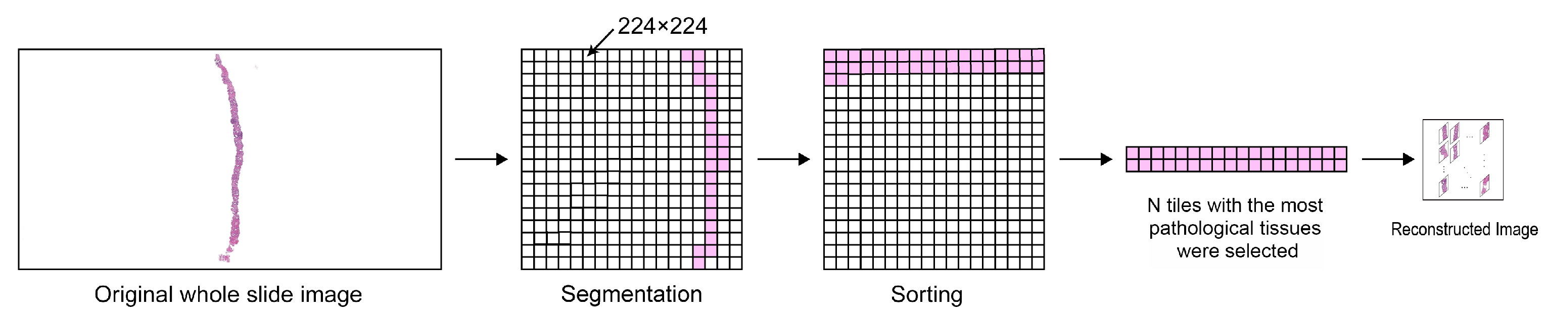
Since the slide images were large and with blank areas that took the majority of space in the image, it was necessary to reduce the image size as well as re-organize the image in a way to zoom in and locate areas of concern. We adopted a strategy similar to the Patch-Based Image Reconstruction (PBIR) method proposed in [8]. Briefly, PBIR works by splitting the original whole-slide image into multiple small patches of different sizes and selecting the patches with more tissues were chosen to reconstruct a new image. Our preprocessing approach consists of two stages. We firstly performed data augmentation on images via 3D rotation, transpose, vertical flip, and horizontal flip; then, for each whole-slide image, we sliced it into patches of 224 × 224 pixels. Out of these tiles, we selected the top 36 most informative ones. The number 36 was empirically chosen to seek a balance between processing speed and model precision. The idea was to keep the tiles with prostate tissues and discard the ones mostly with white background (with a pixel value of 255) that does not have much predictive value to the task. Specifically, we sorted the tiles by the mean pixel value in ascending order, and kept the top 36 tiles that were considered as the most informative ones in the image. The selected tiles were then assembled to form a new image, which served as an input sample used for training. Figure 1 displays the steps of preprocessing that allows the DL model to focus on the areas worth studying.
2.3. Model Framework
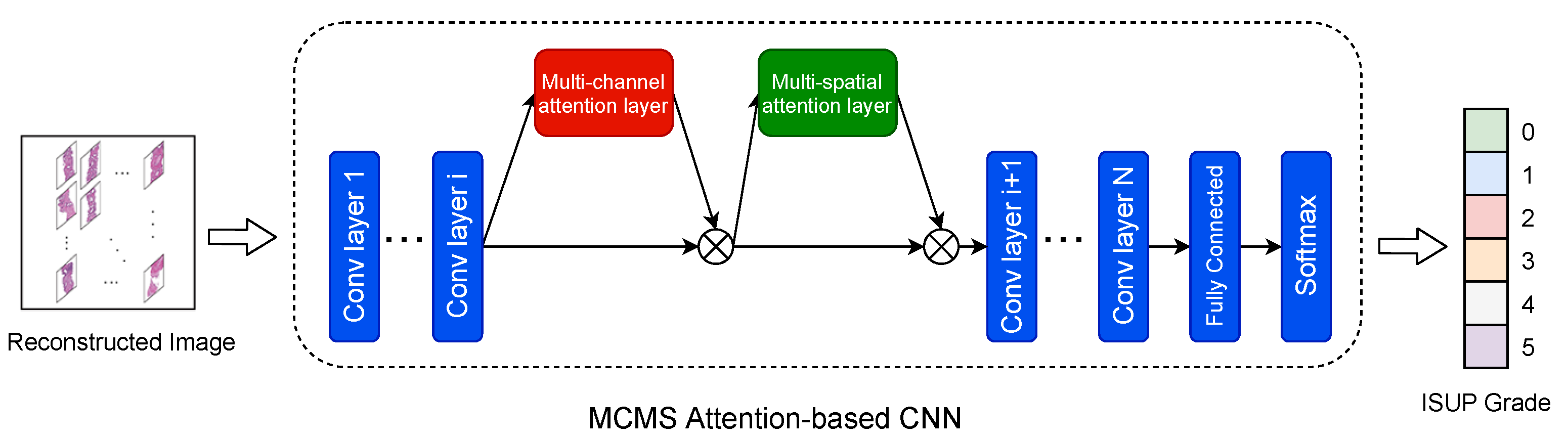
After preprocessing, the restructured images and their labels were trained and validated through our MCMS attention-based CNN model. The proposed MCMS attention module could be plugged into any existing CNN backbone architecture to enhance feature extraction. The multi-channel attention layer allowed the model to learn the most important channel, while the multi-spatial attention layer helped the model learn the most informative areas. Thus, by learning to assign different weights to different channels and spatial areas, the model was trained to identify more distinguishable patterns from the extracted features, eventually making more reasonable predictions and achieving higher accuracy. Figure 2 presents the overall framework of the proposed MCMS attention-based CNN model.
2.4. Multi-Channel and Multi-Spatial Attention Module
This subsection covers the technical details of the MCMS attention module. Given an intermediate CNN feature map , a MCMS attention module sequentially infers a 1D channel attention map and a 2D spatial attention map as shown in Figure 3a,b. The overall process of MCMS attention module can be summarized as:
where ⊗ denotes element-wise multiplication. With different reduction ratios in the multi-channel attention layer and different convolutional kernel sizes in the multi-spatial attention layer, the MCMS attention module enables the backbone network to learn more discriminative features for classifying PCa.
2.4.1. Multi-Channel Attention Layer
The multi-channel attention layer aims to exploit the inter-channel relationship of a feature map. Each channel in a feature map can be considered as a feature detector, and the channel attention determines which feature is more meaningful for the final diagnosis by assigning different weights to different channels.
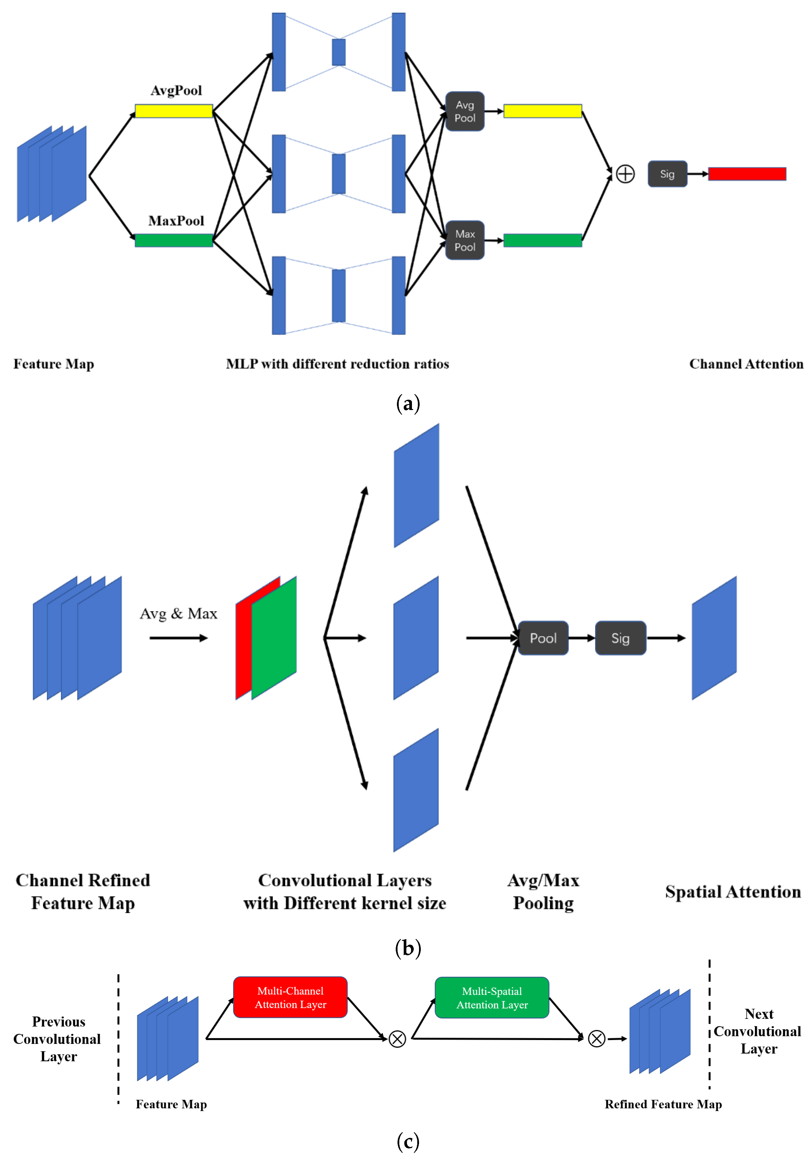
As shown in Figure 3a, spatial information in the given feature map is squeezed by both average and max pooling operations. The results of these two pooling operations can be denoted as and (both in ), which are then fed into several multi-layer perceptrons (MLP), each having one hidden layer. To reduce the parameter overhead, a reduction ratio is set for the ith MLP that produces a hidden activation in . The intuition is that MLPs with different reduction ratios could extract more diversified channel attention vectors. The MLPs in multi-channel attention layer are defined as , , …, , where m is the number of reduction ratios. Outputs of these MLPs are first merged using channel-wise maximization and average operations, and further merged through an element-wise summation, and eventually pass through a sigmoid function to generate a channel attention . Finally, we obtain a refined feature map through a channel-wise multiplication operation between the channel attention and the original feature map , as shown in Equation (1).
2.4.2. Multi-Spatial Attention Layer
The multi-spatial attention layer, following the channel attention layer, aims to mine the inter-spatial relationship of features so as to better identify and focus on the most distinguishable and informative areas of an input image.
As shown in Figure 3b, the refined feature map is firstly applied to produce two one-channel feature maps and that are in . These two feature maps are concatenated along the channel axis as the input to multiple parallel convolutional layers with different kernel sizes. The output feature map of each convolutional layer can encode where to emphasize or suppress, where i is the index of convolutional layer and is the corresponding kernel size. Intuitively, the choice of applying different kernel sizes could potentially produce richer attention information. The output feature maps of these convolutional layers are concatenated along the channel axis to produce a set of feature maps denoted as , where m is the number of parallel convolutional layers. then passes through an average or max pooling layer along the channel axis to produce or in , which is followed by a sigmoid function for generating the spatial attention map . The final output feature map of the MSMS attention module is , which is given in Equation (2).
3. Experimental Validation
This section covers the experimental details, including the choice of performance metrics, the hyper-parameters used in training, and the baseline model.
3.1. Evaluation Metrics
The evaluation metrics that we adopted in this work were accuracy (ACC) and the quadratic weighted kappa (QWK). Briefly, ACC measures the percentage of correct predictions on the test data. As shown in Equation (3), it can be calculated by dividing the number of correct predictions, including true positives (TPs) and true negatives (TNs), by the number of total predictions, namely, the test set size. On the other hand, QWK is used to measure the amount of similarity between predictions and ground truth. The definition of QWK involves the following elements for an N-class classification problem: O is an histogram matrix (i.e., the confusion matrix) where corresponds to the number of ISUP grade i that receives a predicted value j; W is an matrix of weights that represent the differences between actual and predicted values, and is given in Equation (4); E is another histogram matrix of expected outcomes calculated as the outer product between the actual rating’s histogram vector and the predicted rating’s histogram vector. Both E and O are normalized such that each has a sum of 1. Equation (5) shows that how QWK can be calculated. QWK is more informative than ACC when working with imbalanced data. For our task, Table 1 shows that samples with ISUP grades 0 and 1 are more than the rest samples combined, indicating a moderate imbalanced sample distribution. To this end, QWK was chosen as the secondary performance metric.
3.2. Implementation Details
3.2.1. Preprocessing
The original whole-slide images were randomly selected for data augmentation. Each image had a 50% chance to be augmented via a series of operations, including transpose, vertical flip, and horizontal flip. We then sliced each whole-slide image into square tiles that were , out of which 36 most informative ones were selected after sorting all tiles by the mean pixel value. The lower the mean pixel value was, the more prostate tissue information a tile had. The selected 36 tiles were combined to form a new image with the most valuable pixel information kept. These new images, along with the original labels, were used to train our model.
3.2.2. Model Training
Since the proposed MCMS attention module is designed to be plug-and-play, a backbone network is needed for validation. In our experiments, we chose ResNet50 as the backbone CNN, where the MCMS attention module can be plugged into certain convolutional layers. For training an MCMS-assisted ResNet50, we set the batch size to 15 and the start learning rate to 3e-4, with a warmup factor of 10. Three reduction ratios 16, 32, and 64 were used in the multi-channel attention layer, and three kernel sizes, including 3, 5, and 7, were used in the multi-spatial attention layer. The choice of reduction ratios and kernel sizes was based on empirical results.
3.2.3. Baseline
The Convolutional Block Attention Module (CBAM) [23] was set as the baseline in our experiment. CBAM employs both channel and spatial attention layers. It is also a plug-and-play module that can boost the representation power of CNNs. CBAM-assisted CNNs showed consistent improvement on multiple benchmarks, including ImageNet-1K, MS COCO, and VOC 2007. In the experiments, the reduction ratio of CBAM was set to 16 for the channel attention layer, and convolutional kernel size was set to 7 in the spatial attention layer.
4. Results and Analysis
In this section, we report the experimental results by comparing the performance of different models on the PANDA dataset. The models that were evaluated are described as follows:
- ResNet50 and ResNet101 are two popular ResNet [24] variants, with 50 layers and 101 layers deep, respectively.
- To keep a consistent CNN architecture, we chose ResNet50 as the backbone network, and integrated the CBAM or MCMS into the backbone to create various models. For CBAM, two models, including CBAM-Layer4 and CBAM-Layer3 and 4, were evaluated; the CBAM-Layer4 had the CBAM module integrated into the fourth convolutional layer, and CBAM-Layer3 and 4 had the CBAM module integrated into the third and fourth layers.
- For MCMS, four models, including MCMS-Layer4-MAX, MCMS-Layer3 and 4-MAX, MCMS-Layer4-AVG, and MCMS-Layer3 and 4-AVG, were evaluated, in which the MAX/AVG suffix in the model names specify the pooling operation applied to the outputs of the parallel convolutional layers within the multi-spatial attention layer.
Our empirical results showed that adding the attention module to the early layers of the backbone network was more effective, indicating that the low-level features play a more crucial role in building a strong model. Table 2 shows the performance of tested models in ACC and QWK. The observations and insights are highlighted as follows:
- ResNet101 outperformed ResNet50 by 1.2% in ACC, and was on a par with ResNet50 in QWK, meaning that simply adding more layers to the ResNet has limited effect.
- The improvement led by the attention module was significant. With one CBAM block added, CBAM-Layer4 outperformed ResNet101 by 1.7% in ACC and by 1.78% in QWK. Our best model, MCMS-Layer3 and 4-AVG outperformed ResNet101 by 4.18% in ACC and by 7.64% in QWK.
- Adding the attention module to multiple layers of the backbone network brought marginal improvement, and this was the case for both CBAM and MCMS, with an average improvement of 0.52% and 1.29%, in ACC and QWK, respectively. The results were from a comparison of CBAM-Layer3 and 4 vs. CBAM-Layer4, MCMS-Layer3 and 4-MAX vs. MCMS-Layer4-MAX, and MCMS-Layer3 and 4-AVG vs. MCMS-Layer4-AVG.
- We observed that an averaging pooling was more effective than a max pooling when aggregating the outputs of the convolutional layers within the spatial attention layer, with an average improvement of 0.59% and 5.02%, in ACC and QWK, respectively, after a comparison of MCMS-Layer4-MAX vs. MCMS-Layer4-AVG and MCMS-Layer3 and 4-MAX vs. MCMS-Layer3 and 4-AVG. Intuitively, a max pooling is better at extracting sharp, dark, and extreme features, while an average pooling encourages the network to identify all discriminative regions of an object [25]. Our task was benefit from pooling over activations across several pooling neighborhoods, and an average pooling gave a strong signal in middle and soft edges, leaving us with more information on where the edges of the feature were localized, which was lost with max pooling.
- A fair comparison between CBAM and MCMS is CBAM-Layer3 and 4 vs. MCMS-Layer3 and 4-AVG, and results showed that the latter outperformed the former by 1.5% in ACC and by 3.71% in QWK, demonstrating the efficacy of adopting multiple reduction ratios and convolutional kernel sizes.
5. Discussion
DL has been recognized as a revolutionary technology that creates an explosive impact on all industries. Recent advances have explored the potential of DL-based models on cancer diagnosis [26]. As the second most common cancer among men worldwide, PCa diagnosis is not efficiently done due to a worldwide shortage of proficient pathologists. DL has become the mainstream technique behind the latest automated PCa grading systems, which significantly speed up PCa diagnosis and treatment. However, a key challenge of building an accurate grading system is to allow a DL model to learn what and where to extract the most informative features from a whole-slide image, which is usually with background noise, morphological heterogeneity of slide contents, as well as artifacts. For example, the original whole-slide images in the PANDA dataset are large and in high resolutions, while the part with colored tissue information is like a thin and long belt, only taking up a small percent of the coverage. Moreover, many methods overly rely on massive manual labeling and hand-picked RoIs, but the data available are usually incomplete and with imperfect labels. The proposed MCMS attention module is driven by the need to mining distinguishable features and patterns from a whole-slide image to detect the severity of PCa.
The mission of the MCMS attention module is to empower the backbone CNN to learn the areas of concern, i.e., the channels and spatial locations that carry distinguishable information. This mission is accomplished by assigning optimized weights, namely attentions, to channels and spatial locations, so as to refine the original feature map with the learned attentions. Similar ideas have appeared in prior studies [23,27]. The uniqueness of the proposed MCMS attention module lies in the presence of multiple MLPs with different reduction ratios and multiple convolutional layers with different kernel sizes, which offers a view with finer granularity when attending the input feature map. Due to the structural innovation, MCMS demonstrated superior performance compared to its peers. Results showed that adopting different reduction ratios and kernel sizes did help boost feature extraction, leading to performance elevation in both ACC and QWK.
The proposed MCMS-assisted model can serve as a core component for building an automated PCa grading system. Beyond that, since the attention block allows the model to pinpoint areas of concern in a whole-slide image, the system can be used to train practicing pathologists. For example, an interesting use case would be developing a software tool that can generate image exercises that ask trainees to mark and grade areas of concern, which are then compared with the reference answers generated by the tool. Moreover, a software medical robot can be built to learn from a group of experienced pathologists through active and reinforcement learning, and meanwhile, to teach students with novel and more accurate feature patterns. Such a medical robot will make education more effective, productive, and engaging.
This study is subject to some limitations that also point to future directions. First, we only tested the MCMS module on the slide images with one resolution. A potential improvement is to create a pyramid of images with different resolutions, which could allow the model to generate a pyramid of feature maps that the MCMS module can further refine. Second, the number of reduction ratios in the channel attention layer and the number of kernel sizes in the spatial attention layer, along with their values, can be made as hyper-parameters. An empirical guidance on the choice of these hyper-parameters is worth further investigation. Third, our model was trained on a multi-center PCa dataset, and it would be appealing to evaluate how well the MCMS-assisted model performs on datasets created by other centers and how existing domain adaptation techniques and transfer learning can help minimize the fine-tuning effort. Lastly, although validated through our experiments, a deeper interpretation of the MCMS module from the learning theory perspective would benefit the design of new attention mechanisms in the future.
Author Contributions
Conceptualization and methodology, B.Y. and Z.X.; software, validation, and original draft preparation, B.Y.; review and editing, supervision, Z.X. All authors have read and agreed to the published version of the manuscript.
Funding
This research received no external funding.
Institutional Review Board Statement
Not applicable.
Informed Consent Statement
Not applicable.
Data Availability Statement
The prostate cancer grade assessment dataset supporting the conclusions of this article are available at https://www.kaggle.com/c/prostate-cancer-grade-assessment (accessed on 20 March 2021).
Acknowledgments
I must express my sincere appreciation to Rentao Gu, (School of Information and Communication Engineering, Professor of Beijing University of Posts and Telecommunications), my advisor, for his continued support and valuable guidance in the process of planning, experiment and writing. My gratitude also goes to Yan Li, (Department of urological surgical, QiLu Hospital of ShanDong University) for his editorial suggestions.
Conflicts of Interest
The authors declare no conflict of interest.
References
- Bray, F.; Ferlay, J.; Soerjomataram, I.; Siegel, R.; Torre, L.; Jemal, A. Global cancer statistics 2018: GLOBOCAN estimates of incidence and mortality worldwide for 36 cancers in 185 countries (vol 68, pg 394, 2018). CA Cancer J. Clin. 2020, 70, 313. [Google Scholar]
- Samaratunga, H.; Delahunt, B.; Yaxley, J.; Srigley, J.R.; Egevad, L. From Gleason to International Society of Urological Pathology (ISUP) grading of prostate cancer. Scand. J. Urol. 2016, 50, 325–329. [Google Scholar] [CrossRef] [PubMed]
- Ström, P.; Kartasalo, K.; Olsson, H.; Solorzano, L.; Delahunt, B.; Berney, D.M.; Bostwick, D.G.; Evans, A.J.; Grignon, D.J.; Humphrey, P.A.; et al. Artificial intelligence for diagnosis and grading of prostate cancer in biopsies: A population-based, diagnostic study. Lancet Oncol. 2020, 21, 222–232. [Google Scholar] [CrossRef]
- Copeland, A.R.; Kass, M.E.; Crawford, J.M. Adequacy of Pathology Resident Training for Employment: A Survey Report from the Future of Pathology Task Group/In Reply. Arch. Pathol. Lab. Med. 2007, 131, 1767. [Google Scholar] [CrossRef] [PubMed]
- Egevad, L.; Delahunt, B.; Samaratunga, H.; Leite, K.R.; Efremov, G.; Furusato, B.; Han, M.; Jufe, L.; Tsuzuki, T.; Wang, Z.; et al. The International Society of Urological Pathology Education web—A web-based system for training and testing of pathologists. Virchows Arch. 2019, 474, 577–584. [Google Scholar] [CrossRef] [PubMed] [Green Version]
- Li, J.; Li, W.; Gertych, A.; Knudsen, B.S.; Speier, W.; Arnold, C.W. An attention-based multi-resolution model for prostate whole slide imageclassification and localization. arXiv 2019, arXiv:1905.13208. [Google Scholar]
- Xu, H.; Park, S.; Hwang, T.H. Computerized classification of prostate cancer gleason scores from whole slide images. IEEE/ACM Trans. Comput. Biol. Bioinform. 2019, 17, 1871–1882. [Google Scholar] [CrossRef] [PubMed]
- Xie, H.; Zhang, Y.; Wang, J.; Zhang, J.; Ma, Y.; Yang, Z. Automated Prostate Cancer Diagnosis Based on Gleason Grading Using Convolutional Neural Network. arXiv 2020, arXiv:2011.14301. [Google Scholar]
- Ilse, M.; Tomczak, J.; Welling, M. Attention-based deep multiple instance learning. In Proceedings of the International Conference on Machine Learning, PMLR, Stockholm, Sweden, 10–15 July 2018; pp. 2127–2136. [Google Scholar]
- Hussain, L.; Ahmed, A.; Saeed, S.; Rathore, S.; Awan, I.A.; Shah, S.A.; Majid, A.; Idris, A.; Awan, A.A. Prostate cancer detection using machine learning techniques by employing combination of features extracting strategies. Cancer Biomark. 2018, 21, 393–413. [Google Scholar] [CrossRef] [PubMed]
- Regnier-Coudert, O.; McCall, J.; Lothian, R.; Lam, T.; McClinton, S.; N’Dow, J. Machine learning for improved pathological staging of prostate cancer: A performance comparison on a range of classifiers. Artif. Intell. Med. 2012, 55, 25–35. [Google Scholar] [CrossRef] [PubMed] [Green Version]
- Pinckaers, H.; Bulten, W.; van der Laak, J.; Litjens, G. Detection of prostate cancer in whole-slide images through end-to-end training with image-level labels. arXiv 2020, arXiv:2006.03394. [Google Scholar]
- Nirthika, R.; Manivannan, S.; Ramanan, A. Loss functions for optimizing Kappa as the evaluation measure for classifying diabetic retinopathy and prostate cancer images. In Proceedings of the 2020 IEEE 15th International Conference on Industrial and Information Systems (ICIIS), Rupnagar, India, 26–28 November 2020; pp. 144–149. [Google Scholar]
- Farjam, R.; Soltanian-Zadeh, H.; Jafari-Khouzani, K.; Zoroofi, R.A. An image analysis approach for automatic malignancy determination of prostate pathological images. Cytom. Part B Clin. Cytom. J. Int. Soc. Anal. Cytol. 2007, 72, 227–240. [Google Scholar] [CrossRef] [PubMed]
- Gorelick, L.; Veksler, O.; Gaed, M.; Gómez, J.A.; Moussa, M.; Bauman, G.; Fenster, A.; Ward, A.D. Prostate histopathology: Learning tissue component histograms for cancer detection and classification. IEEE Trans. Med Imaging 2013, 32, 1804–1818. [Google Scholar] [CrossRef] [PubMed] [Green Version]
- Nguyen, K.; Jain, A.K.; Sabata, B. Prostate cancer detection: Fusion of cytological and textural features. J. Pathol. Inform. 2011, 2. [Google Scholar] [CrossRef] [PubMed]
- Campanella, G.; Silva, V.W.K.; Fuchs, T.J. Terabyte-scale deep multiple instance learning for classification and localization in pathology. arXiv 2018, arXiv:1805.06983. [Google Scholar]
- Hou, L.; Samaras, D.; Kurc, T.M.; Gao, Y.; Davis, J.E.; Saltz, J.H. Patch-based convolutional neural network for whole slide tissue image classification. In Proceedings of the IEEE Conference on Computer Vision and Pattern Recognition, Las Vegas, NV, USA, 27–30 June 2016; pp. 2424–2433. [Google Scholar]
- Zhang, G.; Wang, W.; Yang, D.; Luo, J.; He, P.; Wang, Y.; Luo, Y.; Zhao, B.; Lu, J. A bi-attention adversarial network for prostate cancer segmentation. IEEE Access 2019, 7, 131448–131458. [Google Scholar] [CrossRef]
- Nagpal, K.; Foote, D.; Liu, Y.; Chen, P.H.C.; Wulczyn, E.; Tan, F.; Olson, N.; Smith, J.L.; Mohtashamian, A.; Wren, J.H.; et al. Development and validation of a deep learning algorithm for improving Gleason scoring of prostate cancer. NPJ Digit. Med. 2019, 2, 1–10. [Google Scholar] [CrossRef] [PubMed] [Green Version]
- Epstein, J.I.; Egevad, L.; Amin, M.B.; Delahunt, B.; Srigley, J.R.; Humphrey, P.A. The 2014 International Society of Urological Pathology (ISUP) consensus conference on Gleason grading of prostatic carcinoma. Am. J. Surg. Pathol. 2016, 40, 244–252. [Google Scholar] [CrossRef] [PubMed]
- Arvaniti, E.; Fricker, K.S.; Moret, M.; Rupp, N.; Hermanns, T.; Fankhauser, C.; Wey, N.; Wild, P.J.; Rueschoff, J.H.; Claassen, M. Automated Gleason grading of prostate cancer tissue microarrays via deep learning. Sci. Rep. 2018, 8, 12054. [Google Scholar] [CrossRef] [PubMed]
- Woo, S.; Park, J.; Lee, J.Y.; Kweon, I.S. Cbam: Convolutional block attention module. In Proceedings of the European Conference on Computer Vision (ECCV), Munich, Germany, 8–14 September 2018; pp. 3–19. [Google Scholar]
- He, K.; Zhang, X.; Ren, S.; Sun, J. Deep residual learning for image recognition. In Proceedings of the IEEE Conference on Computer Vision and Pattern Recognition, Las Vegas, NV, USA, 27–30 June 2016; pp. 770–778. [Google Scholar]
- Zhou, B.; Khosla, A.; Lapedriza, A.; Oliva, A.; Torralba, A. Learning deep features for discriminative localization. In Proceedings of the IEEE Conference on Computer Vision and Pattern Recognition, Las Vegas, NV, USA, 27–30 June 2016; pp. 2921–2929. [Google Scholar]
- Munir, K.; Elahi, H.; Ayub, A.; Frezza, F.; Rizzi, A. Cancer diagnosis using deep learning: A bibliographic review. Cancers 2019, 11, 1235. [Google Scholar] [CrossRef] [PubMed] [Green Version]
- Hu, J.; Shen, L.; Sun, G. Squeeze-and-excitation networks. In Proceedings of the IEEE Conference on Computer Vision and Pattern Recognition, Salt Lake City, UT, USA, 18–22 June 2018; pp. 7132–7141. [Google Scholar]
Figure 1.
An overview of our data preprocessing method. Firstly, we apply image augmentation to the original whole-slide images to enhance the dataset diversity. We further slice each image into smaller tiles in , followed by a sorting of these tiles based on the mean pixel value. The top N (N = 36 in this study) most informative ones are selected to form a new image, which is a -tile square image.

Figure 2.
An overview of the MCMS attention-based CNN for whole-slide image classification. We take the preprocessed images with their labels as input to train a CNN with the MCMS module added after a selected convolutional layer to learn channel and spatial attentions. The feature map is refined with the attention information and passes through the network to enhance feature representation. After training, the model is able to quickly zoom in areas of concern and outputs an ISUP grade.

Figure 3.
The proposed MCMS attention module consists of a multi-channel attention layer and a multi-spatial attention layer and can be easily plugged into any CNN backbone network with minimum change in the code level. (a) Multi-Channel Attention Layer; (b) Multi-Spatial Attention Layer; (c) MCMS attention module integrated with a convolutional layer.


Table 1.
The statistical information of the PANDA dataset.
| ISUP Grade | Train | Test |
|---|---|---|
| 0: background (non tissue) or unknown | 2314 | 578 |
| 1: stroma (connective tissue, non-epithelium tissue) | 2133 | 533 |
| 2: healthy (benign) epithelium | 1074 | 269 |
| 3: cancerous epithelium (Gleason 3) | 996 | 248 |
| 4: cancerous epithelium (Gleason 4) | 1000 | 249 |
| 5: cancerous epithelium (Gleason 5) | 979 | 245 |
Table 2.
Results of model evaluation in ACC and QWK.
| Model | ACC | QWK |
|---|---|---|
| ResNet50 | 0.6638 | 0.7766 |
| ResNet101 | 0.6761 | 0.7739 |
| CBAM-Layer4 | 0.6931 | 0.7917 |
| CBAM-Layer3 and 4 | 0.7029 | 0.8132 |
| MCMS-Layer4-MAX | 0.7093 | 0.7913 |
| MCMS-Layer3 and 4-MAX | 0.7102 | 0.7992 |
| MCMS-Layer4-AVG | 0.7133 | 0.8411 |
| MCMS-Layer3 and 4-AVG | 0.7179 | 0.8503 |
Publisher’s Note: MDPI stays neutral with regard to jurisdictional claims in published maps and institutional affiliations. |
© 2021 by the authors. Licensee MDPI, Basel, Switzerland. This article is an open access article distributed under the terms and conditions of the Creative Commons Attribution (CC BY) license (https://creativecommons.org/licenses/by/4.0/).
Share and Cite
MDPI and ACS Style
Yang, B.; Xiao, Z. A Multi-Channel and Multi-Spatial Attention Convolutional Neural Network for Prostate Cancer ISUP Grading. Appl. Sci. 2021, 11, 4321. https://doi.org/10.3390/app11104321
AMA Style
Yang B, Xiao Z. A Multi-Channel and Multi-Spatial Attention Convolutional Neural Network for Prostate Cancer ISUP Grading. Applied Sciences. 2021; 11(10):4321. https://doi.org/10.3390/app11104321
Chicago/Turabian StyleYang, Bochen, and Zhifeng Xiao. 2021. "A Multi-Channel and Multi-Spatial Attention Convolutional Neural Network for Prostate Cancer ISUP Grading" Applied Sciences 11, no. 10: 4321. https://doi.org/10.3390/app11104321
Note that from the first issue of 2016, this journal uses article numbers instead of page numbers. See further details here.