2.2. Slit Lamp Images
The photos had been taken by two trained clinicians with a digital slit lamp microscope (Topcon SL-D4 slit-lamp biomicroscope). For all the participants, the following protocol was used for photography: 1. We illuminated with a halogen lamp, with a 7.5 KLux illumination input to the slit lamp (both red-free and diffuser filters excluded) and with a wide diffuse illumination of a slit lamp (8 mm circle); 2. We adopted a magnification of 16×; 3. We used a 14 mm diaphragm aperture; 4. We set the sensibility of the digital image to 100 ISO; 5. We set the acquisition time to 1/80 s. All the photographs were acquired under similar room illumination.
For taking images of the nasal and temporal bulbar conjunctiva, each participant was instructed to look horizontally left and right. Gentle pressure was applied to open the lids in order to ensure that they did not obstruct the conjunctiva during the photography. Photographs were taken without flash and quickly to avoid dry eye and irritation.
The images of the GD were collected during clinical practice by the clinicians without standardized parameters of acquisition (such as brightness): each clinician acquired the image according his best judgment, as it is standard clinical procedure.
All of the images were captured in a raw format, i.e., RGB 8-bit, and saved in JPEG format (2576 × 1934, 150 dpi, 24 bit).
2.3. Clinical Scoring of Images
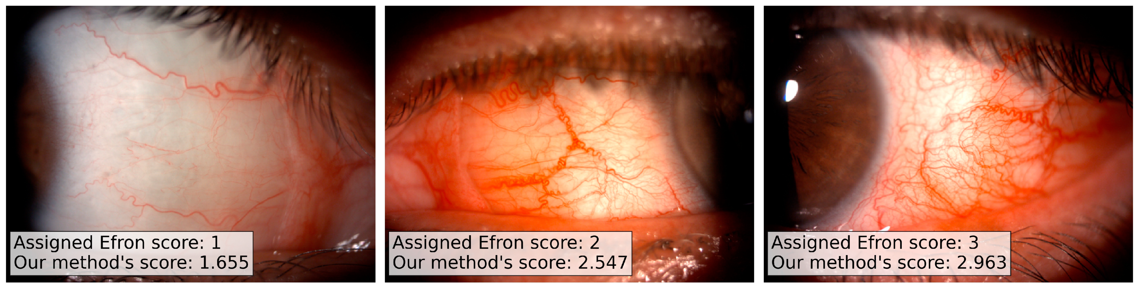
Three trained clinicians performed the evaluation of the full set of 280 images, independently. The clinicians scored each image according to the Efron grading scale: despite the 5 possible values of the Efron scale (from normal, 1, to severe, 5), we allowed the usage of intermediate values in case of doubt. We have chosen the Efron scale as reference since it is a standard reference in ophthalmology and its automation can easily encourage the clinicians community to use our method.
All of the clinicians scored the images in the same physical space, with the same source of illumination and without time limits. Two computer monitors (HP Z27 UHD 4K, 27″, 3840 × 2160 resolution) were used: the first displayed the grading scale images (reference) and in the second one the clinical images were showed. In both of the monitors, the same screen color and brightness were used for all the three clinical evaluations.
We collected the evaluation of the three trained clinicians on the full set of images, and we kept the median value as ground truth score for the analysis.
2.4. Image Processing Pipeline
Our image processing pipeline is composed by a series of independent and fully automated steps (ref.
Figure 1):
conjunctiva segmentation;
vessels network segmentation;
vessels network features extraction and color features extraction;
Efron scale values prediction.
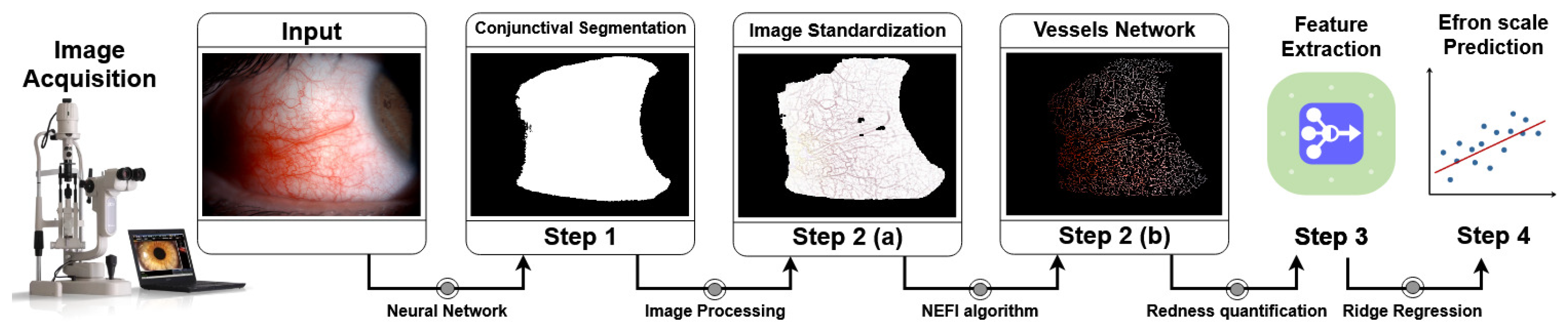
Figure 1.
Schematic representation of the pipeline. (Step 1) The image acquired by the slit lamp is used as input for the Neural Network (Mobile U-Net) model for the segmentation of the conjunctival area. The model was trained using manually annotated images validated by experts. (Step 2(a)) Focusing on the conjunctival area the image is standardized using a brighter-correction algorithm given by a combination of median filters and background subtraction. (Step 2(b)) The image standardization helps us to remove possible artifacts and color issues related to the non-rigid image acquisition procedure. The processed image is used as input for the vessels network segmentation algorithm given by a tuned implementation of the NEFI algorithm. (Step 3,4) Starting from the vessels’ network image, a set of features for the quantification of the conjunctival redness are extracted and used for the development of a predictive model. The full set of steps are performed automatically and thus without any human intervention.
![Applsci 11 02978 g001]()
The first step of processing involves the segmentation of the conjunctiva area from the background, i.e., skin, eyelids, eyelashes, and caruncle. For each image of the datasets, we collected a manual annotation of the conjunctiva area performed and validated by the 3 experts. The manual annotation set includes a binary mask of the original image in which only the conjunctiva area is highlighted. The conjunctiva segmentation allows for reducing the region of interest of our analysis on the most informative area for the redness evaluation.
Several already published automated grading systems for the hyperemia quantification perform this step using semi-supervised methods, leaving to the final user the manual selection of the region of interest (ROI) [
3,
8,
9,
10]. Our method automatizes this task using a semantic segmentation neural network model trained on a set of images manual annotated and validated by experts.
In the second step, the pipeline performs a second segmentation for the vessels’ network identification, starting from the segmented conjunctiva. The vessels network is automatically segmented using a customized version of the NEFI [
19] algorithm. The vessels network segmentation provides a mask to apply to the original image.
In step three, the pipeline extracts features starting from the selected areas based on quantities proposed in the literature and based on different color spaces (RGB and HSV, i.e., Hue, Saturation, and Value). In step four, the extracted set of features was used to feed a penalized regression model for the prediction of the final Efron scale value.
2.4.1. Step 1—Conjunctiva Segmentation
In literature, there are several deep learning models proposed to automate the segmentation of eyes’ images (e.g., optical coherence tomography [
20], sclera segmentation [
21,
22,
23], retinal vessel [
24]); nevertheless, we could not find any model focusing on slit lamp images. These images are theoretically easy to segment since the purpose is to isolate the white-like part of the image (conjunctiva) from the red-like background (skin, eyelids, eyelashes, and caruncle), but in reality the differences between these two regions are not uniform in the different parts of the same image and not as well defined in the color space. An image thresholding [
10] or an image quantization [
9] could solve this task in the simplest cases, but they can not take care of the extremely variability of the samples provided by a clinical acquisition. There is not a rigid standardized procedure in the image acquisition by a slit lamp during the clinical acquisition and the “elaboration” of the images is left to the experience of the clinicians.
In our work, we divide the available image samples into a training (42 patients, 60% of the full set of images, i.e., 168 images) and a validation set (28 patients, 40% of the full set of images, i.e., 112 images). From the training set, we excluded a subset of 18 images, i.e., 9 patients, as test set for the evaluation of the model performances over the training procedure. For each image, we collected a manual annotation of the conjunctiva area performed and validated by 3 experts. The manual annotation set includes a binary mask of the original image in which only the conjunctiva area is highlighted; this set of images-masks was used as ground truth for our deep learning model.
The amount of the available samples does not justify the usage of a complex deep learning architecture with a large amount of parameters to tune. During the research exploration, we tried several CNN architectures commonly used in segmentation tasks, starting from DenseNet CNN to the lighter U-Net variants [
25,
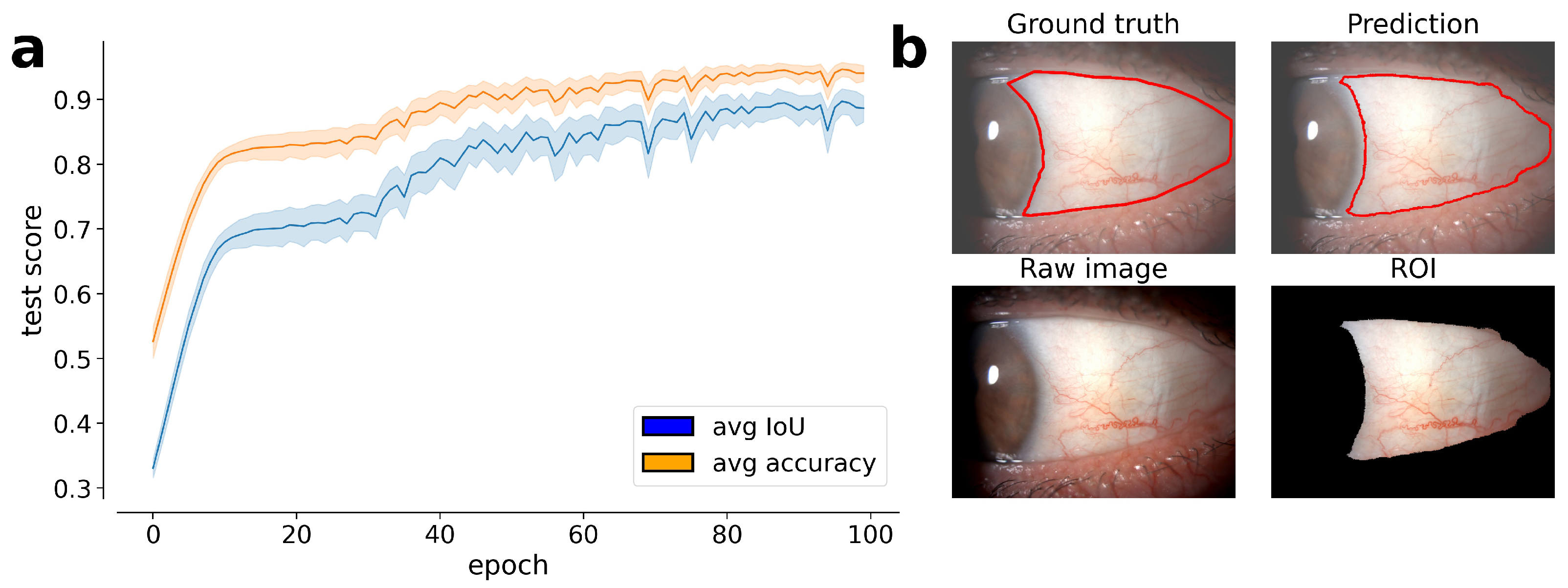
26]. The evaluation of model performances has to balance both a good performance on the validation set and a greater ability of extrapolation on new possible samples. We would like to stress that, despite the above requirements being commonly looked for in any deep learning application, they are essential for any clinical application, in which the variability of the samples is extremely high. We remark that even high accuracy scores could still include distortions and artifacts of clinical significance: the most important result is the clinician’s evaluation, i.e., the visual segmentation accuracy estimated by experts. All of the predicted images were carefully evaluated by the experts of the Ophthalmology research group of the IRCCS S. Orsola University Hospital Ophthalmic Unit, Laboratory for Ocular Surface Analysis of the University of Bologna and their agreement, jointly with the training numerical performances, lead us to choose a Mobile U-Net model with skip connection as the best model able to balance our needs.
We implemented the Mobile U-Net model using the Tensorflow Python library. The model was trained for 100 epochs with an RMSProp optimizer (learning rate of and decay of ). For each epoch, we monitored the accuracy score, i.e., the average agreement between the mask produced by the model and the ground truth at pixel level, and the Intersection-Over-Union (IoU) score, i.e., the area obtained by the union of the mask produced by the model and the ground truth divided by their intersection area, on each image of the test set. Since the portion of the image occupied by the conjunctiva area could be smaller compared to the full image size, the IoU score is a more informative metric for the evaluation of the model performances since it is robust to unbalances in the sample, differently from the accuracy score. Our training set includes both nasal and temporal images for both the patient eyes. This means that we have an intrinsic vertical flip of the training images. We however performed a large data augmentation procedure to build a more robust model and to hypothesize the possible variability of the test set. For each image, we performed a vertical and/or a horizontal flip jointly with a random rotation.
2.4.2. Step 2—Vessels Network Segmentation
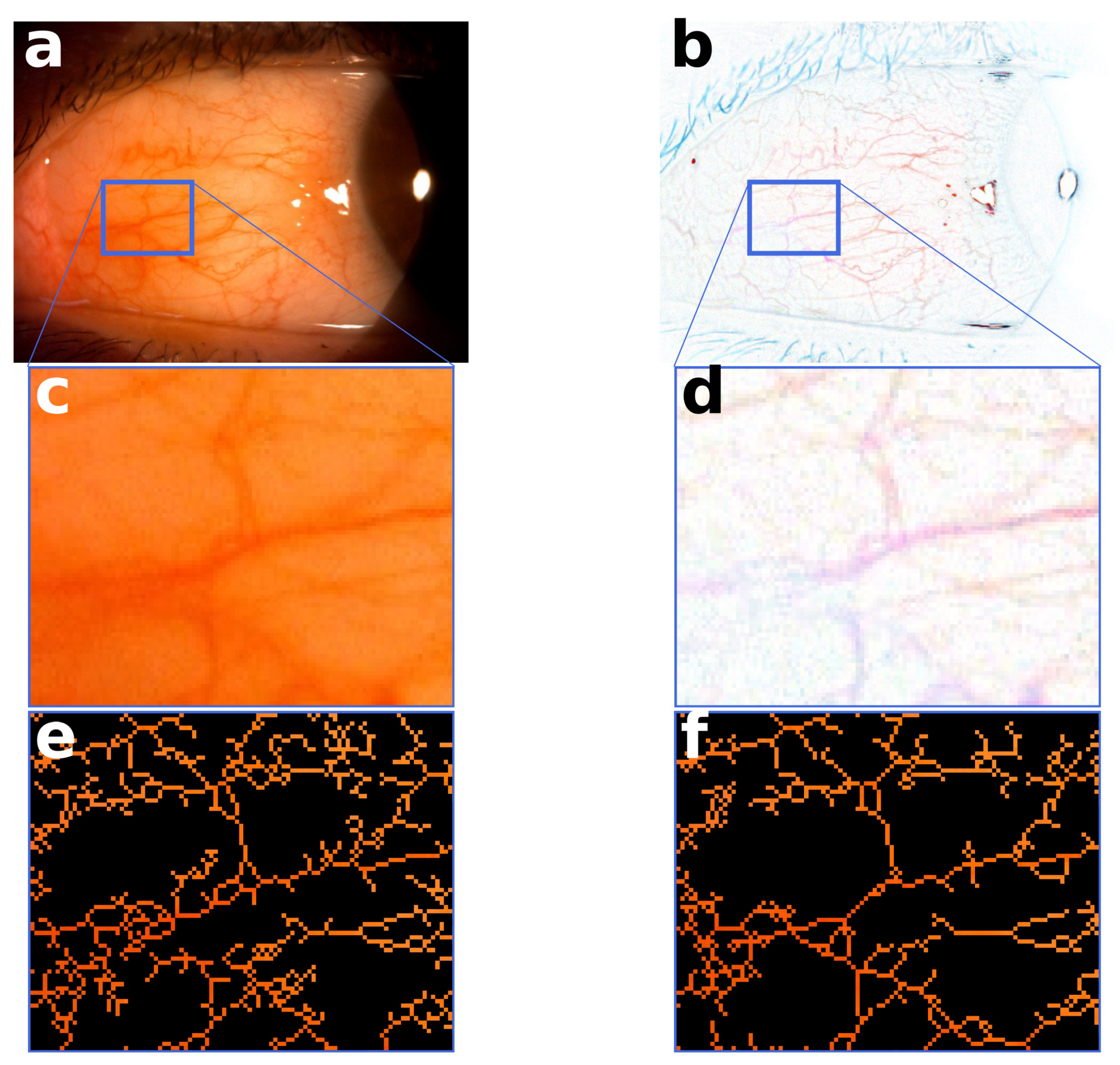
The conjunctiva segmentation allows for reducing the region of interest of our analysis on the most informative area for the redness evaluation. The first step of processing involves a standardization of the images and the correction of the light dependence due to uneven illumination of the conjunctiva. In the same image, different parts of the conjunctiva could have different brightness based on the angle of the incidental light on the conjunctiva and the aperture of the slit lamp diaphragm. This different brightness produces images with a shadow component or with a flash glare. The vessels network in the conjunctiva can thus appear as a brighter or a darker red component, and this can drastically affect the redness evaluation. The images, in fact, tend to appear with a heterogeneous red component when the acquisition is performed in low-light situations. At the same time, the light standardization allows for removing the possible shadows or hyper-intense areas due to the effect of the flash over the patient’s eyes. This standardization is performed independently on each channel of the image (R, G, and B), and it involves a median blurring of the channels followed by a normalization of the difference between the blurred and the original channel. The resulting standardized image is converted into grayscale before the application of the next steps.
Starting from the standardized masks, the pipeline performs the vessel segmentation. The vessels’ network segmentation is a standard task in ophthalmology image processing, and many studies have already published promising results on this topic [
3,
9,
10,
19,
27,
28]. In our work, we decided to use a customized version of the method proposed in [
19], using a watershed adaptive filter to highlight the network vessel component and to segment it from the background. After removing the smaller connected components (up to a predetermined size) to remove noise artifacts, the resulting segmentation is refined using a GuoHall skeletonizer [
29]. In this way, only the backbone (only 1 pixel for each branch) of the vessels network is selected. In the next steps, we use the backbone network as a mask for the extraction of the redness features, focusing our analysis on the smallest but most informative region of the image.
2.4.3. Step 3—Redness Features
The redness measurements are standardly performed on the whole area occupied by the conjunctiva, despite the most informative section being given by the only vessels network component. Therefore, for all the features, only the pixels belonging to the vessels network were included.
RGB Redness
Park et al. propose in [
9] a redness measure given by a combination of the RGB channels. The authors extract this score on the manually segmented conjunctival area without any preprocessing step, obtaining promising results on the prediction of the conjunctival redness. The core assumption behind the relation between this feature and the conjunctival redness is the perception of the red color into the conjunctiva area: the mathematical formula tends to emphasize the R intensity using a weighted combination of the three channels. This starting point is generally true in the major part of slit lamp images, but it can suffer from the image light exposition: the RGB channels do not respond in the same way to the image brightness, and this behavior can affect the robustness of the measure.
In our work, we evaluated the same score using the mask provided by the vessels network segmentation: in this way, we can focus our evaluation of the redness only in the most informative area of the conjunctiva, minimizing possible light exposition artifacts. We also improved this measure applying the preprocessing light standardization. Thus, the first feature extracted is the redness score given by
where we denote with R, G, B the red, green, and blue channels of the standardized image, respectively. The
n value represents the amount of pixels in the mask produced by the conjunctival segmentation step.
HSV Redness
A second interesting feature was proposed by Amparo et al. in [
8]. The authors suggest to move from the RGB color space to the more informative HSV one, i.e., the hue, saturation, and value. This space is more informative than the RGB one since it is capable of being careful about the different light exposure (saturation). The authors also suggested the usage of a preprocessing step for the slit lamp images, including a white-balance correction to overcome possible light exposition issues. Despite their interesting results, they did not show further results on the dependence of their feature to the same image sampled in different light conditions. Their measure uses a combination of saturation and hue for the redness estimation, thus we can preliminarly expect a more robust behavior to image brightness. In addition, in this case, we applied the same computation for the extraction of a second score on our standardized image after the vessels network segmentation:
where
H and
S represent the hue and saturation intensities of the standardized image, respectively.
Fractal Analysis
A third set of measurements were proposed by Schulze et al. in [
10], who performed a fractal analysis from the vessels segmented in the conjunctiva. Our technique for the vessels network segmentation is quite different from theirs, but we can, however, apply fractal analysis for the study of the vessels’ topology. The vessels network can be compared to a fractal structure and thus analyzed using standard measurements of complex systems analysis [
30,
31,
32]. Their evaluation can be very informative from a medical point-of-view, and it fills an opened gap in the clinical practice. The estimation of the fractal dimension of the vessels network could be informative of multiple pathologies, since it quantifies the neo-genesis and the ramification of the vessels in the area of interest. Their relation to the hyperemia is straightforward since the greater the area occupied by the vessels, the greater the conjunctival redness. The core assumption in this case is given by the goodness of the segmentation algorithm used for the vessels network extraction: the algorithm should be able to identify the vessels network in any light exposition or the measures can suffer from false positive or missing detections. In particular, we extracted as putative features the fractal dimension of the vessels network using the box-counting and pixel-counting algorithms. Both algorithms are commonly used methods for the analysis of fractal structures included into images. In our work, we choose a logarithmic set of sizes for the box counting evaluation, and, for each image, the coefficients estimated from the linear interpolation between the box-sizes and the counts were used as features (this line slope is usually referred to as the fractal dimension).
Color Measures
We also computed the averages of the RGB channels and HSV channels of the standardized conjunctival networks, reaching a total of 10 putative features for the redness estimation. There are intrinsic correlations between these features that need to be taken into consideration for the subsequent analyses.
2.4.4. Step 4—Regression Pipeline
The initial step of our regression analysis consists of the standardization of the extracted features. Each feature belongs to a different space/range of values and to combine their values, and we have to rescale all of them into a common range. We rescaled all the features using their median values, normalizing according to the 1st and 3rd quantiles, i.e., a robust scaling algorithm: in this way, we minimize the dependency from possible outliers. Medians and quantiles were estimated on the training set and then applied to the test set to avoid cross contaminations.
The processed set of features is then used in a penalized regression model. We used a penalized ridge regression (or Tikhonov regularization) for the Efron prediction. Ridge regression is a regularized version of the linear regression in which an extra regularization term is added to the cost function, penalizing high values of the coefficients of the regression. In our simulations, we used a penalization coefficient equal to .
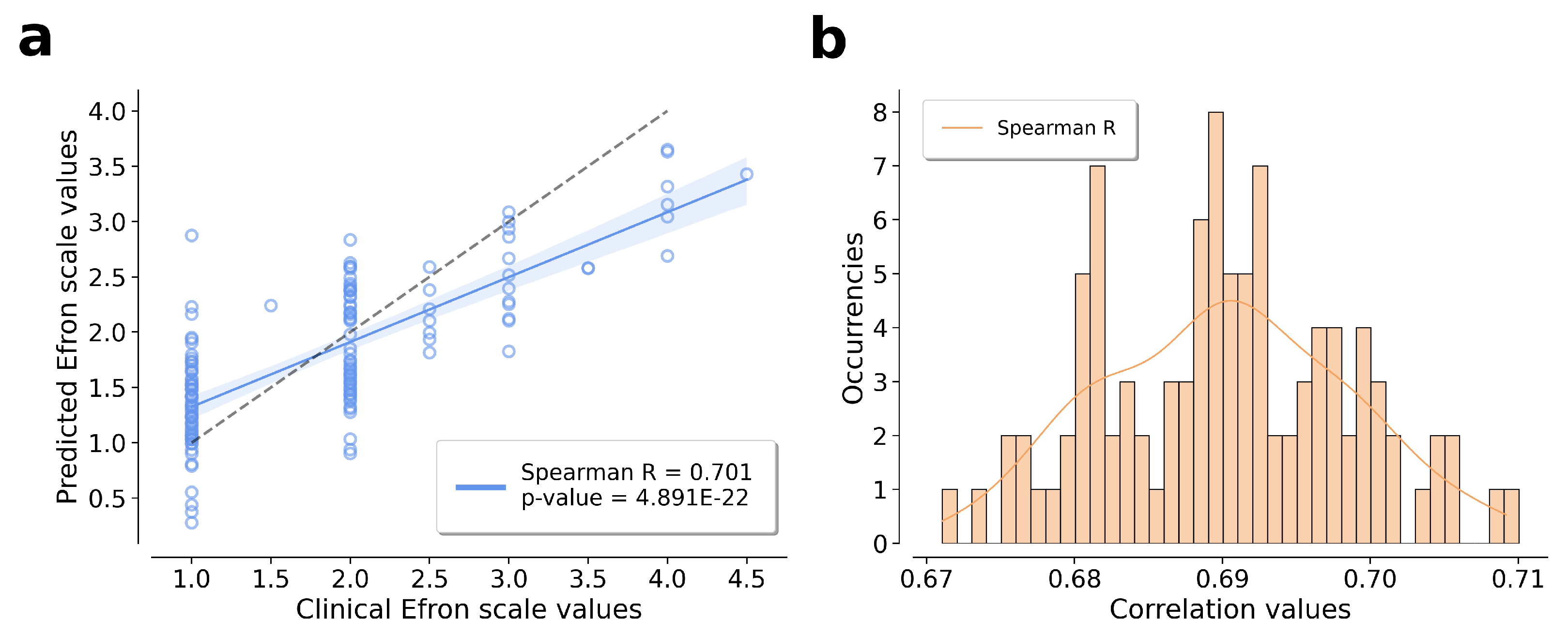
The full set of data was divided into a train/test sets using a shuffled 10-fold cross validation. The model was trained on a subset (90%) of the available samples, and its predictions are compared to the ground truth provided by the corresponding test set (10%).
We want to note that, despite the Efron scale admitting only integer values (from 1 to 5) in our dataset, we have a 8% of floating point values: the experts introduce floating point values when there is no an exact concordance between the patient image and the template image references. We would stress also that the accordance between multiple experts in the Efron scale evaluation is generally low since the measure has an intrinsic subjectivity, and this bounds the best possible predictions of a quantitative model.


 ,
, 


