
Investigating the Dimensional and Geometric Accuracy of Laser-Based Powder Bed Fusion of PA2200 (PA12): Experiment Design and Execution


Department of Manufacturing and Civil Engineering, Faculty of Engineering, NTNU—Norwegian University of Science and Technology, 2815 Gjøvik, Norway
*
Author to whom correspondence should be addressed.
Appl. Sci. 2021, 11(5), 2031; https://doi.org/10.3390/app11052031
Submission received: 29 January 2021
/
Revised: 19 February 2021
/
Accepted: 20 February 2021
/
Published: 25 February 2021
(This article belongs to the Special Issue Mechanical Tolerance Analysis in the Era of Industry 4.0)
Abstract
:Featured Application
The present paper describes the execution of an experiment and the resulting data to facilitate the reuse of experiment results and open research.
Abstract
Variation management in additive manufacturing (AM) is progressively more important as technologies are implemented in industrial manufacturing systems; hence massive research efforts are focused on the modeling and optimization of process parameters and the effect on final part quality. These efforts are, however, hampered by the very problem they are seeking to solve, as conclusions are weakened by poor validity, reliability, and repeatability. This paper details an elaborate experiment design and the subsequent execution with the aim of making the research data available without loss of validity. Test artifacts were designed and allocated to fixed positions and orientations in a grid pattern within the build chamber to facilitate rigid analysis between different builds and positions in the build chamber. A total of 507 specimens were produced over three builds by laser sintering PA12 before inspection with a coordinate measuring machine. This research demonstrates the inherent variations of laser-based powder bed fusion of polymers (LB-PBF/P) that must be considered in experiment designs to account for noise factors. In particular, the results indicate that the position in the xy-plane has a major influence on the geometric accuracy, while the position in the z-direction appears to be less influential.
1. Introduction
As additive manufacturing (AM) is increasingly used for the manufacture of functional components and assemblies, requirements are imposed on the AM processes with regards to dimensional and geometric accuracy [1]. In the manufacturing industry, quality requirements are formalized in standards, such as ISO 1101 [2] for geometric product specifications (GPS) and ASME Y14.5 [3] for geometric dimensioning and tolerancing (GD&T). These standards provide measures of geometric accuracy—commonly referred to as characteristics—that are crucial to secure a good fit of an assembly and the proper functioning of a product. The ability of AM to achieve tolerances comparable to conventional manufacturing technologies is vital for the continued expansion of AM technologies into the commercial manufacturing industry.
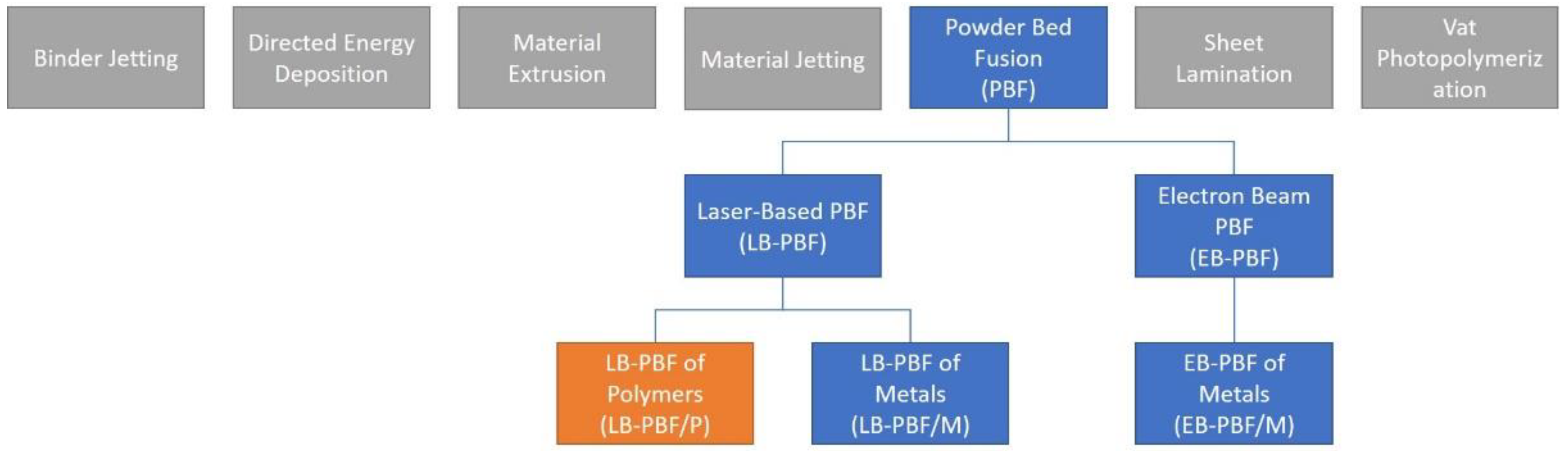
ISO/ASTM 52900:2015 [4] distinguishes seven process categories of AM, all characterized by widely different properties and peculiarities; hence generalization between the technologies is difficult. Due to the inherent differences of the processes, research efforts are often directed towards a single process or a small selection of processes. Although still under rapid development, powder bed fusion (PBF) is one of the more industrialized AM processes and is, therefore, already subjected to the requirements of industry at a larger scale. Further classification of PBF is made by specifying the energy source and material type, i.e., electron beam or laser as the energy source, and metal, polymer, or ceramics as materials, as illustrated in Figure 1 [5]. The current work reports on experiments on laser-based PBF of polymers (LB-PBF/P), popularly known as selective laser sintering (SLS).
Layered manufacturing processes are generally prone to the so-called staircase effect arising from the discretization of a 3D surface into 2.5D layers. This inevitably affects the surface topography and accuracy [6]; hence the phenomena have been modeled in terms of both flatness [7] and cylindricity [8]. Because the severity of the staircase effect depends on the angle of the surface, the surface type plays a major role in how the staircase effect manifests, and therefore, also how the part builds orientation influences the geometric accuracy. In this context, a surface type may be any of the five geometric primitives—plane, cylinder, cone, sphere, and torus—and an occurrence of a surface type on a 3D-model is referred to as a shape feature. Because surface types are influenced differently by part build orientation, the shape features can be used to optimize part build orientation and to predict geometric deviations [9,10].
Previous research has shown that PBF is a complex process with many variables affecting the product in terms of mechanical properties [11,12,13,14,15], surface quality [14,15,16,17,18,19], and geometric and dimensional accuracy [15,20,21,22]. The part build orientation is known to have a significant effect on final quality with regards to all of these areas in addition to its contribution to build time and cost [23]. Consequently, numerous studies include part build orientation as an experimental factor to gauge and model its effect on various measures [24]. While studies on surface roughness in various AM technologies have investigated part build orientations with 10- and 15-degree intervals [19], the effect on dimensional and geometric accuracy is typically not researched with the same level of detail. Baturynska [21] performed a statistical analysis of dimensional accuracy in LB-PBF/P, where four orientations were utilized. Senthilkumaran et al. [25] conducted an experiment in LB-PBF/P with a central composite design where the effect of orientation on flatness and cylindricity was investigated in five levels from 0 to 90 degrees alongside several other factors. Similar studies on other AM technologies are also reported in literature where orientation is typically investigated in 2–5 levels of an experiment design [26,27,28,29].
The driving hypothesis of the present experiment is that the relationship between part build orientation and geometric accuracy is more complex than what can be derived from traditional experiment designs, and more thorough analysis is required. Therefore, the current paper describes an elaborate experiment that is designed and executed to enable a closer analysis of the effects of part build orientation on geometric accuracy.
2. Materials and Methods
The experiment was conducted in five distinct steps as described in the following subsections. First, a test artifact was designed to incorporate the features of interest for the current project. Next, the build layout of three builds was created before the build process started. When the build process was completed, data collection was conducted by employing a coordinate measuring machine (CMM) for accurate and reliable measurements. Finally, the data from the CMM were exported and analyzed.
2.1. Experimental Factors and Strategies
The repeatability of AM experiments is a challenge because the experiments are not only affected by the processing parameters, but studies also indicate that there are major differences between machine types and even between machines of the same make [30,31]. Furthermore, the variations may occur between builds in the same machine and even different positions in the same build [21,32]. It is, therefore, of paramount importance to design rigid experiments by utilizing blocking strategies, or at the very least enable some characterization of such variations. The current experiment applies both blocking and randomizing strategies and replicates all specimens of the main study three times to enable the characterization of variation.
The main purpose of the experiment is to investigate the effect of part build orientation on dimensional and geometric accuracy. In order to obtain data points of adequate density, part build orientations from 0 to 180 degrees are investigated at five-degree intervals around a single axis. To minimize unwanted variations (noise) in the experiment, all variables are kept constant or handled with blocking and randomization strategies, as displayed in Table 1.
In addition to the experimental variable (part build orientation), four variables from Table 1 stand out: (i) placement in build, (ii) build ID, (iii) feature type, and (iv) feature size. It is necessary to produce several specimens simultaneously to complete the experiment within a reasonable time and keep the cost at an acceptable level. A blocking strategy is implemented with regards to the part location in the build to enable linear comparison along the axes of the machine by defining fixed positions in the build space where specimens may be fabricated. The details of the build layout are presented in Section 2.3.
Because the build space is too small to fit three replications of all 37 levels of the experimental variable “part build orientation” in a single build, the experiment must be completed through three separate builds. The variation between builds is handled with a blocking strategy by replicating all part build orientations in every build. Moreover, the three builds were completed in as close succession as possible without interfering with other activities in the laboratory. The environmental conditions were comparable, and the material came from the same batch without any refilling of the powder bins between builds. Details about the build process are presented in Section 2.4, and details on temperature, precipitation and humidity are available in the online repository.
The size of any shape may affect the results of the experiments, especially in AM, where the ratio between the feature size and the layer thickness could significantly affect the deviations of the manufactured surface from the designed surface. It is desired to incorporate shape features of different sizes to investigate how the accuracy varies with feature size; hence several different dimensions are incorporated in the test artifact as described in the following Section 2.2.
2.2. Designing the Test Artifact
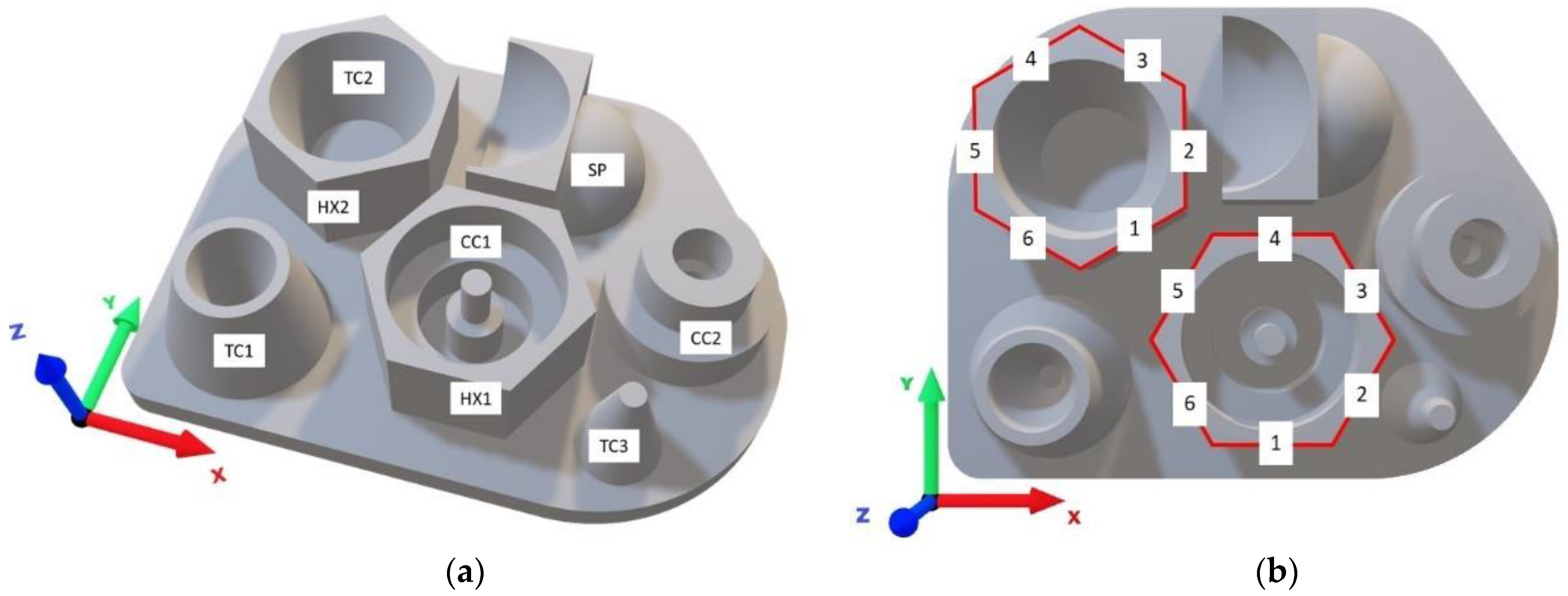
Many benchmark artifacts have been proposed over the years, but few are widely used. For a comprehensive overview of geometric benchmarks for AM, the interested reader is referred to [33]. For the current research, the artifact proposed in [34] was adapted by eliminating redundant features and adding a few elements. The artifact is designed specifically to enable inspection with a CMM and can be manufactured in its original orientation by any current AM technology without the need for support structures. Moreover, the design process was guided by the dimensions of the build space available for the experiment, thus restricting the allowable dimensions of the design. Specifically, it was desired to fit three specimens in their initial build orientation on the same plane in the build space, while maintaining a safe distance between all specimens, as well as between the specimens and the boundaries of the build space (the details on the build layout is presented in Section 2.3.). The feature types selected for the design serve the purpose of gauging the quantitative accuracy of the process rather than the qualitative capabilities. Several dimensions of cylinders and cones are present to enable the analysis of how different feature sizes are affected by the build orientation. The resulting artifact is displayed in Figure 2, where all features are labeled in line with the naming convention of [34], where the elements are assigned a short name based on the surface type and numbered if there are more than one (e.g., CC1 for the first truncated cylinders and SP for the spheres). The artifact was designed in the computer-aided design (CAD) software SolidWorks 2018 and exported as an STL (Stereolithography) file in ASCII-format using deviation tolerances of 0.01 mm and 2°. The artifact was inspected and reoriented to aligned with Cartesian orthogonal axes using Microsoft 3D Builder and converted to binary format. The interested reader is referred to [35] and [36] for details on STL files and the challenges they impose on AM and tolerancing. The artifact is available online, along with all supplementary data.
Following the specifications given in [34], the spherical features (SP) are both 24 mm in diameter, and CC1 and CC2 comprise cylindrical features of the four diameters 4 mm, 8 mm, 16 mm, and 24 mm in both concave and convex form. All cylinders are 8 mm in height to enable inspection with CMM while keeping the dimensions of the artifact at a minimum. The cones in TC1, TC2, and TC3 are all 16 mm tall, with an apex angle of 30 degrees and larger diameters of 12 and 24 mm convex and concave. The HX1 and HX2 are both hexagons extruded 16 mm from the base plate, angled 15 degrees relative to each other, yielding 12 vertical planes in unique orientations evenly distributed from 0 to 275 degrees. All features protrude from a 5 mm thick base plate with rounded corners to minimize the volume of the design. The bounding box of the design is 89.67 mm × 69.24 mm × 21 mm, and the volume of the design is 53,230 mm3. Details on all the elements of the design are available in Table 2.
2.3. Build Layout
The build layout is designed to reduce the required number of builds to conduct the experiment while ensuring acceptable validity. With this in mind, the experiment was designed in three phases as follows:
- Build space segmentation to define fixed positions for specimens in the build space;
- Part location assignment to ensure best validity and repeatability of results; and
- Controlling slice distribution to improve temperature distribution and reduce the risk of failure.
2.3.1. Build Space Segmentation
The build space is first segmented to allow re-orientation of all specimens without violating the required distance between parts. The segmentation serves to define fixed positions in the build space to facilitate comparisons between the different positions and builds in the experiment as this is a known source of variation. This experiment is conducted on an EOSINT P395 with a build volume of 340 × 340 × 620 mm. Due to temperature gradients along the edges of the build envelope, it is recommended to keep a safe distance of 20 mm to the edge, effectively reducing the available build space to a 300 × 300 mm square in the xy-plane. Similarly, it is advisable to keep a certain distance to the bottom of the build space to allow the environment to stabilize (both in terms of temperature and power distribution) before the sintering begins. For this experiment, a safe distance of 6 mm was applied.
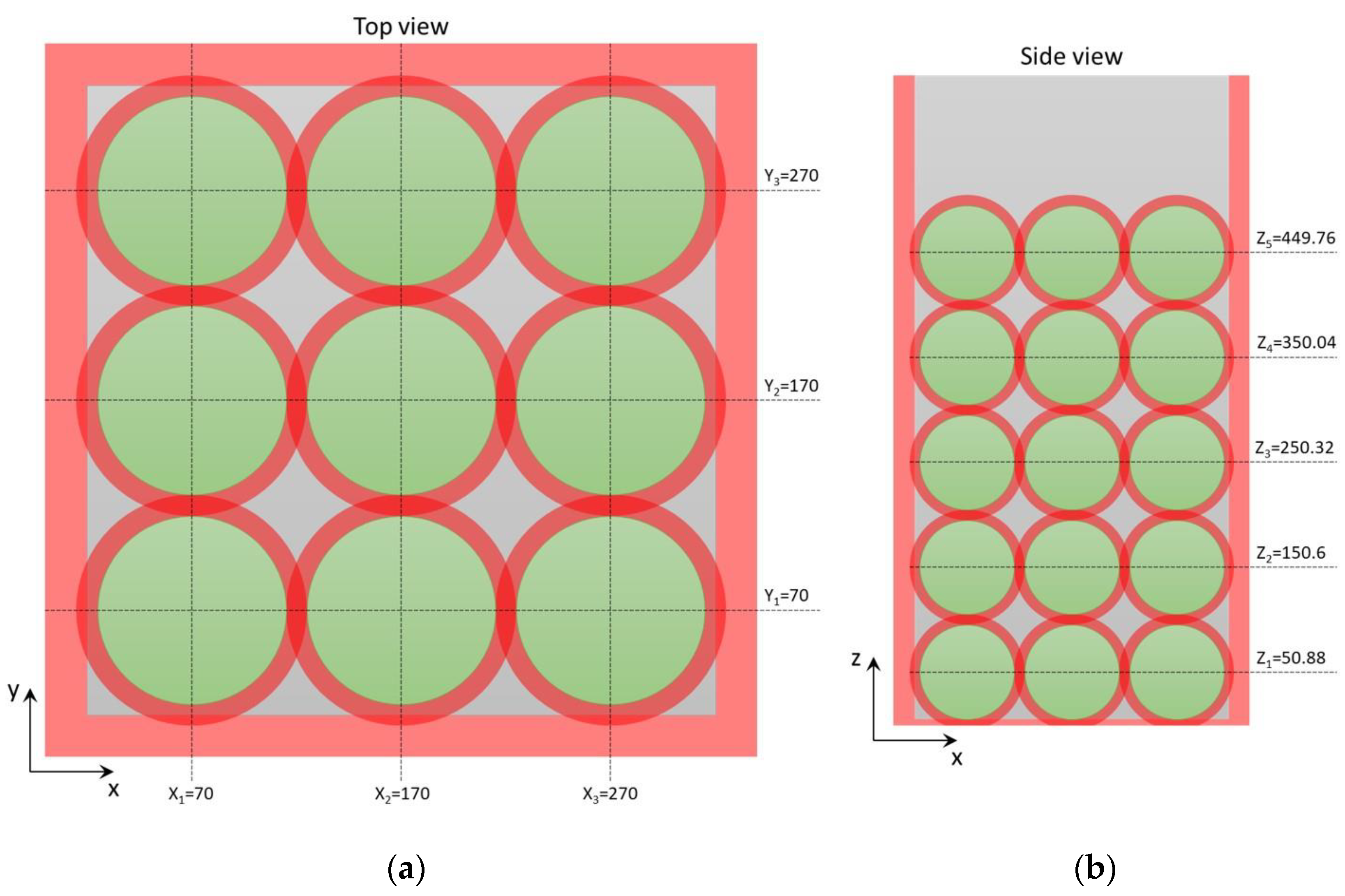
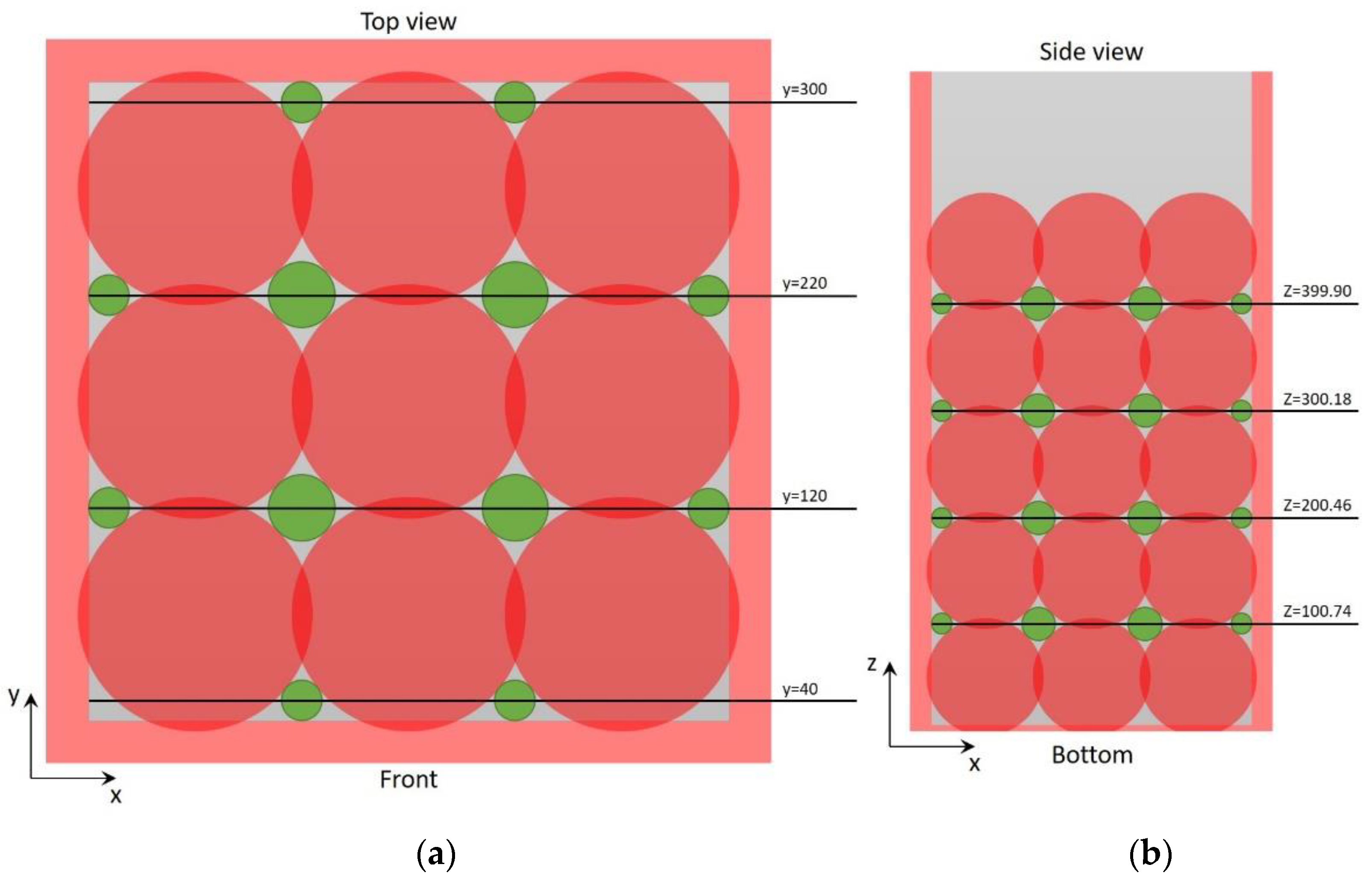
To avoid cross-contamination between specimens in the same build, all specimens should be located at a safe distance from each other. For this experiment, a 10 mm safe zone is considered around all specimens in all directions. The test artifact is designed to fit a grid of three by three specimens in any orientation without violating the safe zone. The first step of build space segmentation is presented as two 2D-projections with a top view in Figure 3a and a front view in Figure 3b. The green discs represent the area potentially occupied by specimens, and red rings encapsulating each disc represent the safe zone. Additionally, the red square frame demarks the safe distance from the edges of the build envelope. The coordinates in the figure are center coordinate components relative to the machine coordinate system [37]. The positions are defined based on the center point at (170, 170), from which the remaining positions are located at the extremes of (170 ± 100, 170 ± 100), i.e., an orthogonal grid with 100 mm distance from center to center. This grid is repeated five times in the z-direction, as illustrated in Figure 3b, yielding a total of 45 defined positions in the build space. These positions may formally be described by three components where , and . The five layers in the z-direction are distributed to account for the required safe distance and adjusted to the closest multiple of the layer thickness (120 µm), resulting in a distance of 99.72 mm from center to center. The lowest center point is determined by finding the lowest viable position that does not violate the 6 mm safe distance from the bottom and then rounding up to the closest multiple of the layer thickness.
2.3.2. Part Location Assignment
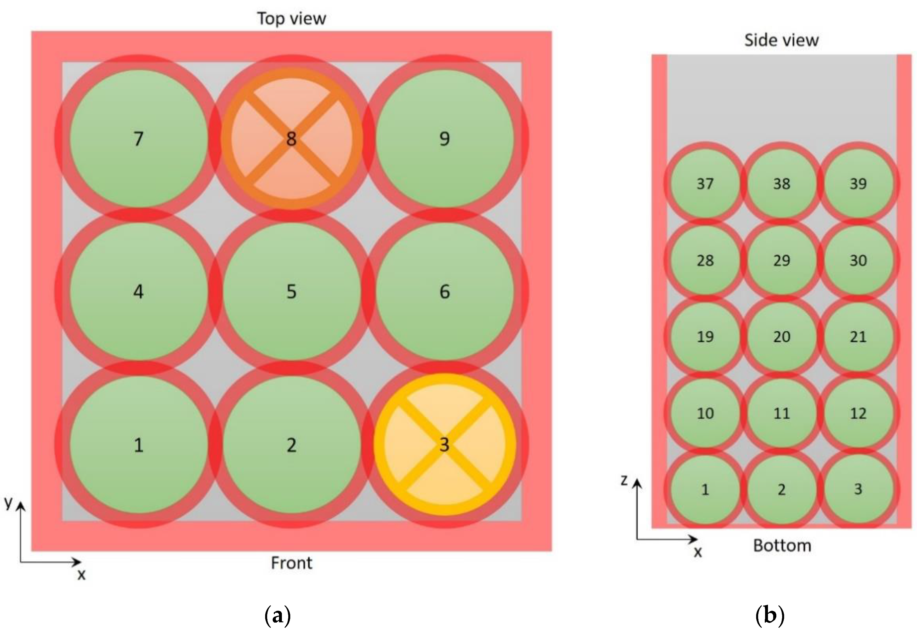
To mitigate systematic errors arising from the position in the build chamber, each specimen is randomly assigned to one of the defined locations in the build space. However, because 45 positions are defined for each build, and only 37 specimens should be produced, a plan must be derived for the remaining eight positions. First, the positions cannot be left open because this could disturb the temperature distribution throughout the build; hence something should be produced in all 45 positions. To ensure that an equal amount of energy is applied to all positions, the same specimen will, therefore, be used to fill this space. Furthermore, these specimens shall not be part of the main study, and they should, therefore, be differentiated from the main group somehow, and it was decided to make the part build orientation 270 degrees about the x-axis—an orientation outside the scope of the main study, while still being somewhat comparable. This allows using these specimen as a control group to further facilitate comparative analyses across builds and positions. In order to keep the variation between the specimens to a minimum, the superfluous positions were restricted to eight defined positions in the build space to be duplicated in all three builds. The rear-center position at (170, 270) for all z-layers was selected because of the assumed similarity to the front-center position (170, 70) and also had the benefit of not being first or last relative to the recoater for any layer. The final three positions excluded from the main study are located in the front-right corner at z-layers 1, 3, and 5. These positions should be similar to the other corners and are evenly distributed along the z-layers to provide evenly distributed data points along this dimension of the build space. The specimens produced at eight extra positions are referred to as “anchor” specimens inspired by their function as fixed data points in the experiment design.
The randomization was conducted in Microsoft Excel by applying the RAND function to assign a floating-point number in the range of [0, 1) to every orientation and then sorting the list with respect to the random number. The list of orientations was then aligned with the list of available positions in the build space, effectively using the list index to determine the position in the build according to the numbering of Figure 4. The assignment of orientations to positions is available in Table A1 in the Appendix A.
The build layout was prepared in the software Materialise Magics 23.01, where the artifact design was imported as a binary STL file, and the mass labeling-function was utilized to create 45 duplicates with the appropriate labeling as displayed in Figure 5. The labeled models were translated to their predetermined position in accordance with the build space segmentation by center coordinates (note that Magics defines the center point of a part as the geometric center of the bounding box). Finally, the models are reoriented into their predetermined part build orientation by counterclockwise rotation about the x-axis.
2.3.3. Controlling Slice Distribution
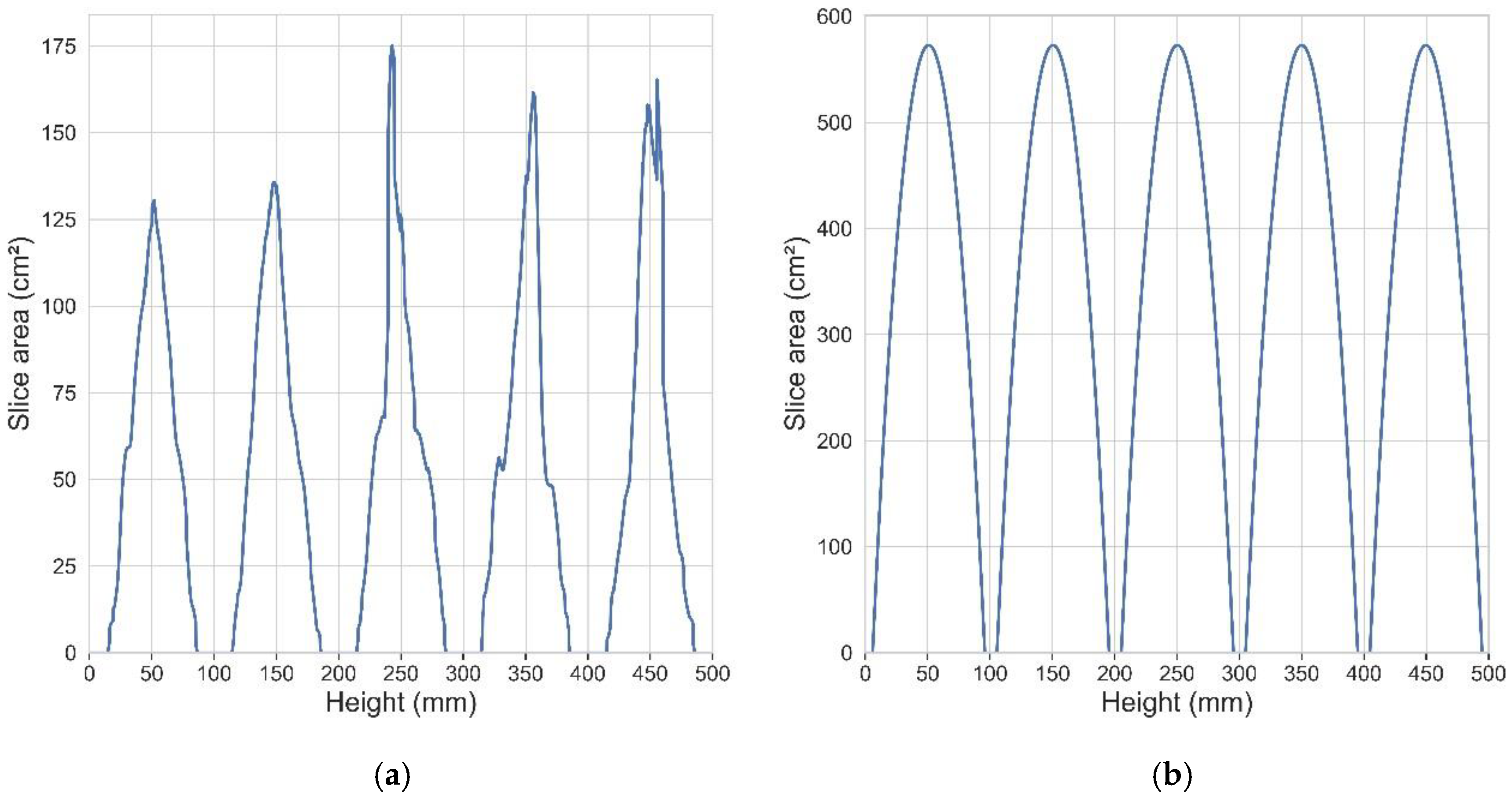
To minimize the risk of machine failure, it is generally recommended to achieve relatively smooth transitions between layers in terms of energy density, i.e., the amount of energy applied to one layer should not deviate too much from the amount of energy applied to the adjacent layers. In practice, this means that parts should preferably be evenly distributed along the build direction or optimally have a uniform intersection area. The cross-sectional area of slices at user-defined intervals can be exported from Magics as an Excel file, effectively yielding the sintered area of each layer. The slice distribution achieved from inserting the specimens of build 1 from Table A1 into the build space yields the graph in Figure 6a, which exhibits large portions without any energy input. These portions without energy input originate from the safe distance between specimens in the z-direction and cannot be eliminated without the introduction of additional specimens. This is demonstrated in Figure 6b, which shows the slice distribution for spheres of 90 mm diameter inserted at the positions of the specimens.
While Figure 6 displays some minor gaps in the slice distribution, the actual layouts of the three builds would be significantly worse because the true geometry of the artifact is much more complex than a perfect sphere, leading to large portions in z-direction without any energy input at all. To counteract the risk associated with the energy fluctuations, one could either change the previously determined positions, or objects could be added to the low-energy volumes to even out the slice distribution. The second option enables additional information to be collected from the experiment by adding useful objects to the unused volumes marked in green in Figure 7.
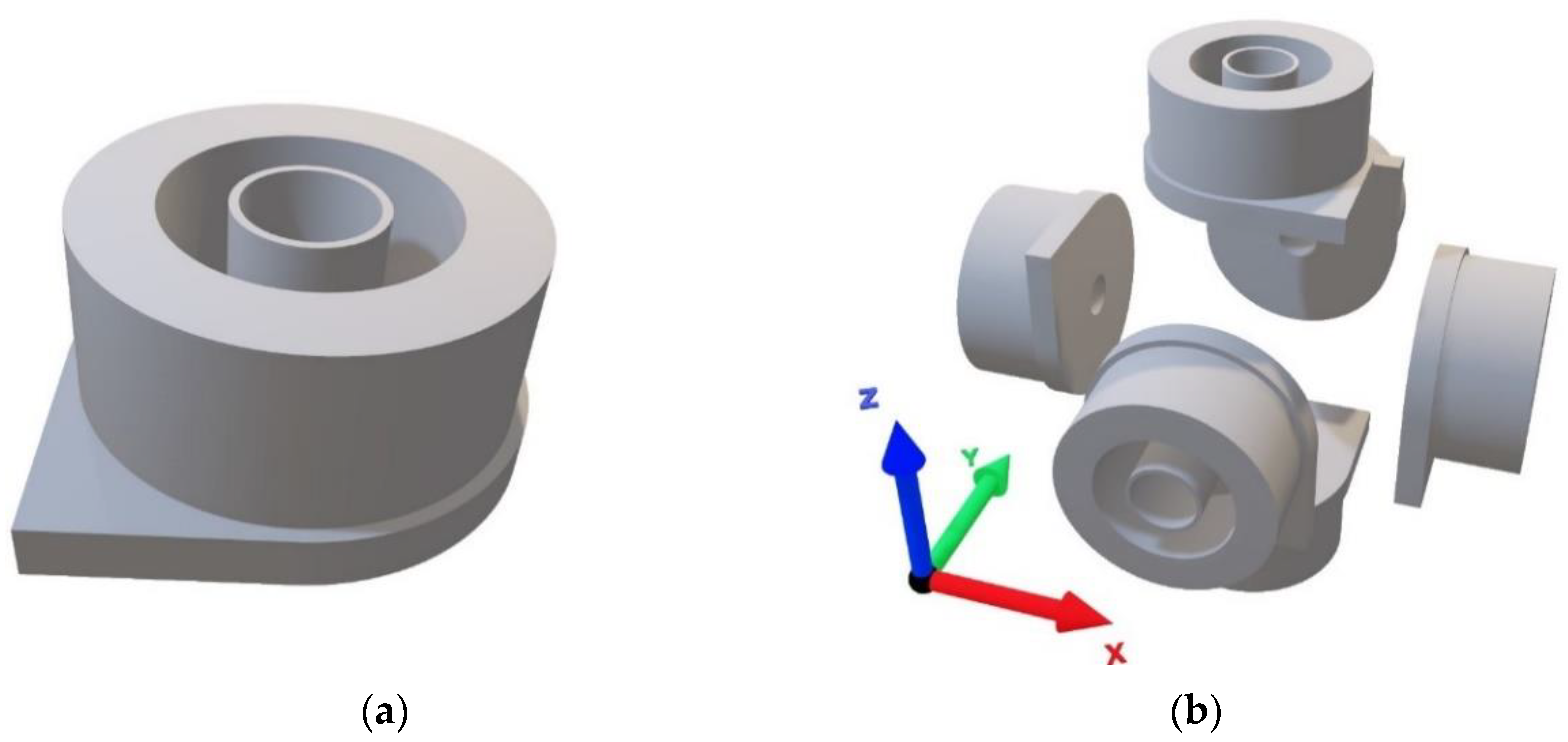
The object inserted in the additional space should be massive enough to significantly contribute to an even slice distribution but also provide additional information that contributes to the validity and reliability of the experiment. The recently developed standard for test artifacts in additive manufacturing ISO/ASTM 52902:2019 [38] provides several candidates in STEP format. The circular artifact CA_F (Figure 8) was selected due to its appropriate size, volume, and feature type. The model was loaded to SolidWorks, exported as a binary STL file, and later duplicated and reoriented in Magics.
With reference to Figure 7, the green areas on the edges of the build volume fit one sample of CA_F each. Therefore, these volumes are used to investigate the effect of the laser angle (as opposed to the build direction), which is shown to be a decisive factor for surface roughness in LB-PBF/M [39]. On each side of the build space, one sample is fabricated with the cylinder orthogonal to the layers, and one sample is adjusted, so the axis of the cylinder points directly towards the laser origin (the last deflection point, i.e., the last mirror before the laser beam enters the build volume). For any point on the powder bed, the laser angle ξ can be expressed as:
where is the vector from the center of the powder bed to the point, is the vector from the laser origin to the point, and and are the magnitudes of the respective vectors. This adjustment assumes that the last mirror is installed 600 mm above the powder bed and precisely in the center, ultimately adjusting the orientation by 13.1 degrees. Table 3 tabulates the positions and re-orientations.
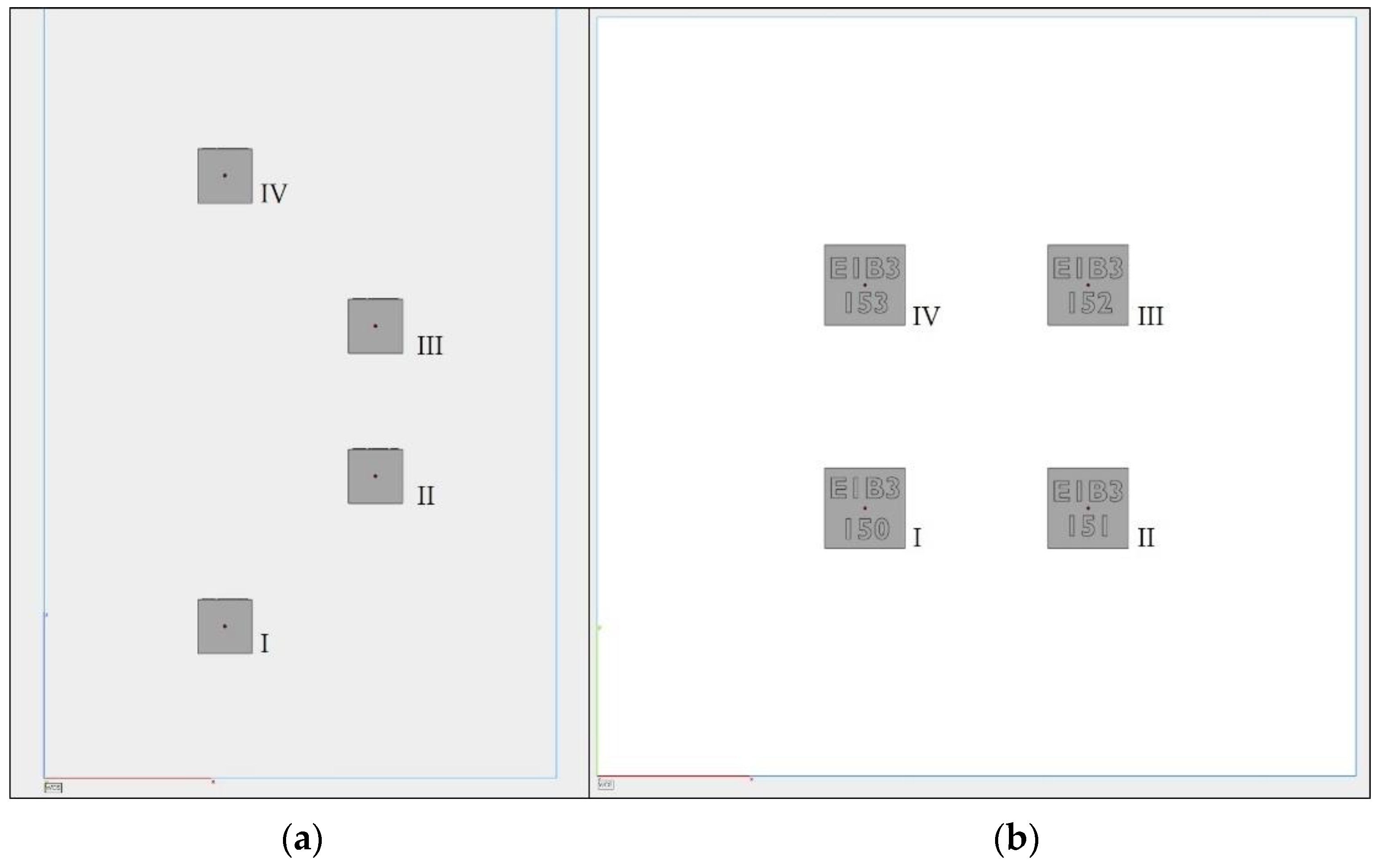
The four empty volumes indicated by green circles in the interior of the build space in Figure 7 are large enough to fit six samples of CA_F pointing in six orthogonal directions each. All specimens of the constellation are located 26.5 mm away from a shared center point to uphold the 10 mm safe zone. This setup is demonstrated in Figure 8b and allows for the investigation of the variations across the build space and between the different builds for a limited number of orientations. This constellation is inserted three of the four volumes, leaving the fourth spot available for a hollow box used to collect powder samples from inside the build. The position of the box is rotated counterclockwise by one-step for each part layer, as displayed in Figure 9.
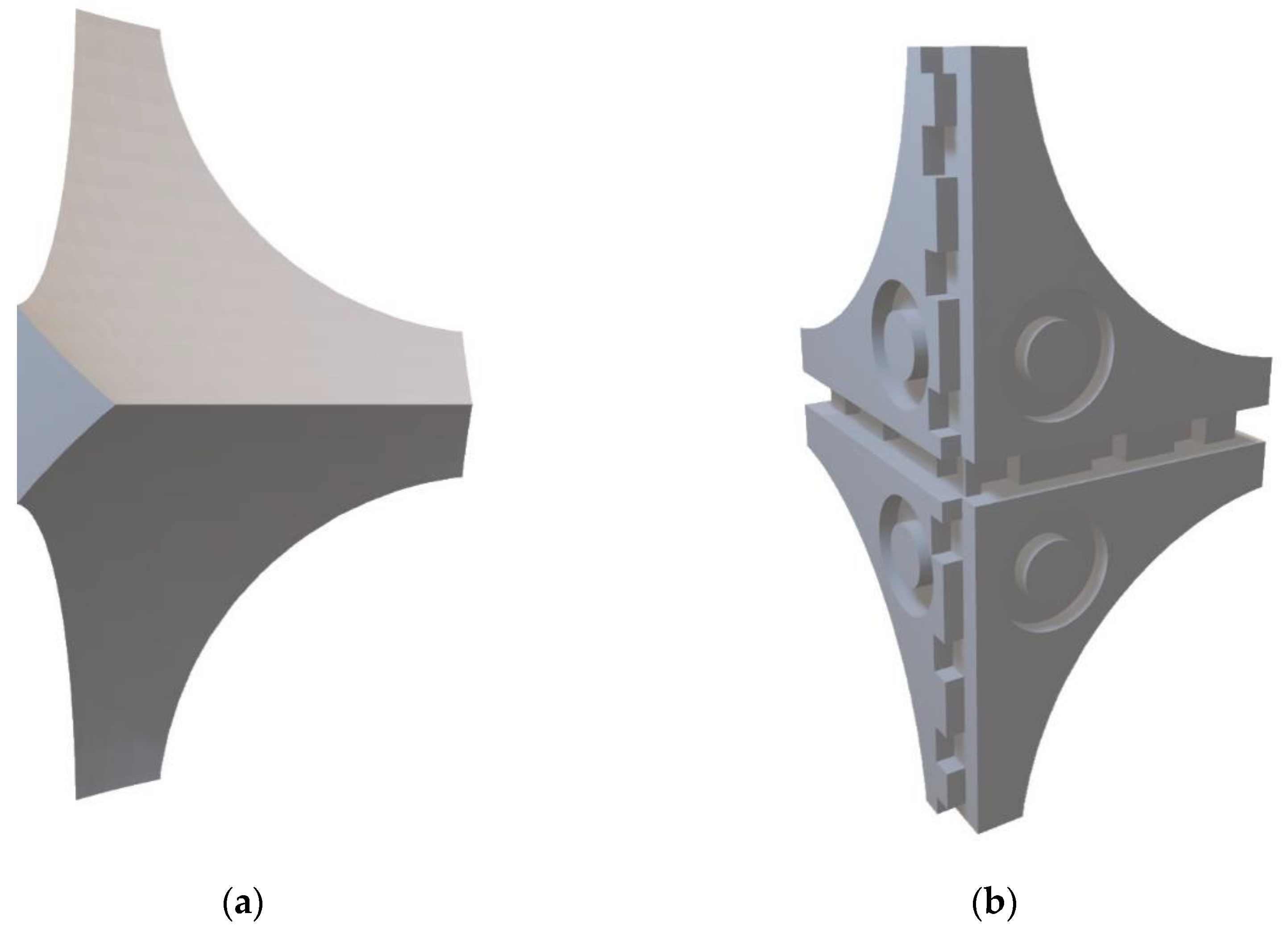
However, the design and constellations are not dense enough to have much of an impact on the slice distribution; hence, yet another artifact was introduced to the layout. At this point, the only viable spaces left in the build volume are the corners of Figure 7, i.e., each of the five layers of main specimens. In order to maximize the utility of the space, an artifact was designed in Microsoft 3D Builder based on the shape of the available volume. This design had the potential to add further value to the experiment, and shapes were, therefore, added to the planar faces of the workpiece. First, the linear artifact LA from ISO/ASTM 52902:2019 [38] is imported and used as a pattern to create imprints in the design. The pattern leaves notches in the back of the specimen of certain intervals along all three axes and allows for measuring the dimensional accuracy on the corners of the build envelope. The remaining area was utilized to add cylinders of 8 and 15 mm in diameter, completing the design in Figure 10. These specimens are inserted at the four z-levels indicated in Figure 7 with four specimens on each level—one in each corner rotated, so the large planar surfaces are parallel with the walls of the build chamber, only leaving the safe distance of 20 mm.
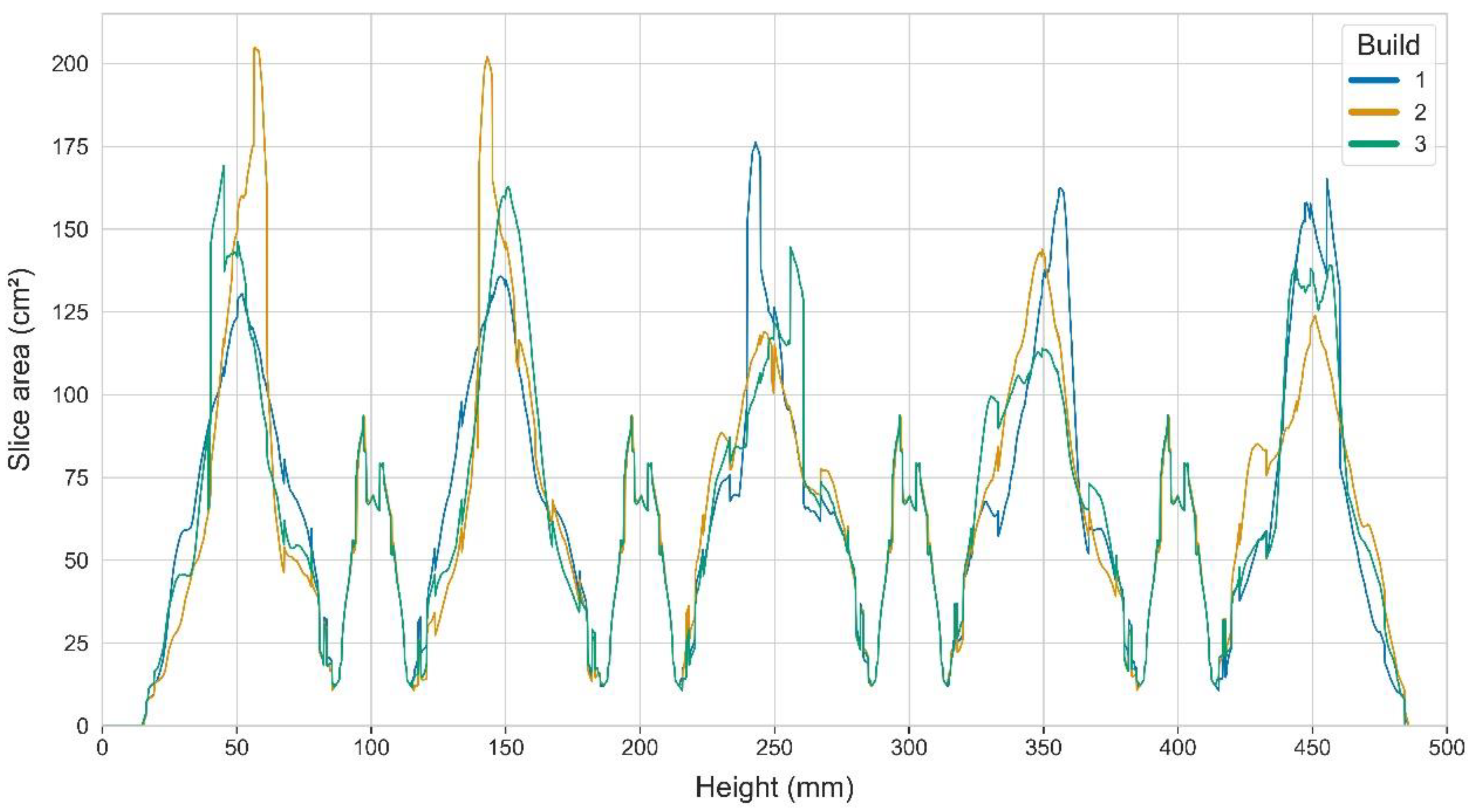
The final layout includes a total of 169 specimens per build: 45 replications of the main specimen, of which 37 replicates are part of the main study and the remaining eight are anchor specimens, 104 replicates of CA_F, of which 72 are part of constellations, and 32 replicates are located along the edges of the build space, 16 duplicates of the corner artifacts and four hollow boxes for powder samples. When the layout design was completed, the Magics “fix” function was utilized to automatically detect and repair STL file errors, such as inverted normals, holes, and intersecting triangles. The slice distributions of all three builds after insertion of the additional parts are shown in Figure 11, the labeling scheme for the additional parts is displayed in Figure 12, and the three builds are displayed in Figure 13.
2.4. Build Process
The specimens were manufactured through three runs with an EOSINT P395 situated at AddLab at NTNU in Gjøvik. The layout described in Section 2.3 was exported to the EOS process software (PSW), where the parameter profile “balanced” was selected with a layer thickness of 120 µm as a typical tradeoff between build time and quality. The powder bins were filled with EOS powder PA2200 (PA12). All virgin powder originated from the same batch, and the machine was fed with a 50/50 blend of virgin and recycled powder. The specifics are summarized in Table 4. The build cycle took roughly 36 h to complete and needed another 36 h to cool before the part cake could be extracted. All specimens were removed from the part cake by hand before pressurized air was used to remove excess powder. After treatment, the specimens are stored in a container in the posttreatment facility to ensure minimum environmental influence.
2.5. Data Collection
This section describes the data collection related to the main study and, therefore, only considers the main specimen while the additional specimens are left for future work. For maximum precision, the specimens were inspected with a Zeiss DuraMax CMM with a measurement accuracy of 2.9 µm + L/200 at 18–30 °C where L is the measurement length in mm. A fixture was designed and 3D-printed to automate the inspection, ensure specimens were measured under the same conditions, and make the changeover from one specimen to the next as simple as possible. The fixture was printed with PLA using a Prusa MK2.5 fused-filament fabrication (FFF) printer with a layer thickness of 0.1 mm. The fixture makes use of a small bolt to secure the specimen against the opposite corner, and the force is carefully exerted on the specimen to avoid deflection, which could influence the results. The fixture was tested with a prototype of the specimen 3D-printed with PLA filament prior to the fabrication of the actual test specimens. This preliminary test displayed negligible deflection when the bolt was tightened by hand and was, therefore, considered appropriate for the current experiment. This decision is further substantiated by the material properties as PLA is significantly more flexible than PA12 and, therefore, more prone to deflection. Figure 14 shows the CAD-design of the fixture (a) and the fixture with the prototype in place (b). The two ears allow the fixture to be bolted to the measurement table with M10 bolts.
2.5.1. Establishing a Base Alignment
Before the measurement can start, an inspection plan must be devised and programmed. This step was completed at the CMM with the accompanying computer running the Zeiss proprietary software Calypso 6.6. The CAD-model is first imported as a STEP file for efficient feature extraction before a base alignment is established to determine the position and rotation of the specimen in space. The base alignment is necessary to teach the CMM where the specimen is located so that it can continue an inspection in automatic mode. In fact, the base alignment lay the foundation for all machine movement in CNC-mode, potentially causing the probe to crash if not correctly defined. The base alignment is typically determined based on the part function and/or the production method using the so-called 3–2–1 principle where a plane (defined by a minimum of three points), a line (minimum two points), and a point is used to define the spatial translation and rotation of a part. However, because the test artifact has no real purpose and the nature of the process inaccuracies are unknown, the following considerations are made regarding which features to utilize: (i) the features should be contained within a single surface/element (i.e., a line stretching across several planes are not recommended); (ii) the features should be located close to the center of the part to counter dimensional accuracies; and (iii) planar features are preferred because they are generally easier to clean and residual powder is more easily detectable. Consequently, the base plate was selected as the plane for base alignment and also defined the origin for the z-axis, a line is drawn on the second plane of HX2, which also defines the origin for the x-axis, and finally, a point is taken on the fourth plane of HX1, which also defines the origin for the y-axis. Figure 15 illustrates the probing points used for the manual alignment conducted at the beginning of every inspection. Because this is a manual task, variation is inevitable, and the red discs of Figure 15 differ in size to reflect the area available for the manual probing. After the manual alignment, the CMM switches to CNC-mode and repeats the alignment before the inspection is automatically completed.
2.5.2. Defining the Inspection Strategy
When the base alignment is established, the features of interest may be extracted from the CAD-model to define tolerance characteristics and determine inspection strategies. The entire inspection is conducted with a single stylus of 3 mm diameter, effectively filtering out surface roughness and other minor surface imperfections. The inspection makes use of scanning strategies where the stylus tip is dragged along the surface while taking points at a high-frequency without compromising the accuracy. This allows a high number of points to be registered, which increases the resolution of the measurements and, therefore, also the reliability of the results. Furthermore, the path of the stylus is designed to cross the build layers of the specimen regardless of part build orientation, which enables detection of defects arising from the layered nature of LB-PBF and is of particular importance for the current experiment. Among all the points collected from a scanned surface, the first points are disregarded to safeguard against inertia and any lingering vibrations. Consequently, it is preferred to inspect each feature with a single undisrupted path covering the largest possible surface area. Naturally, a tradeoff must be made between execution time and the accuracy/resolution of the inspection. For continuity, all features belonging to the same group are treated equally with regards to the stylus path, even though the number of points or the measurement speed must be corrected to make up for the dimensional differences.
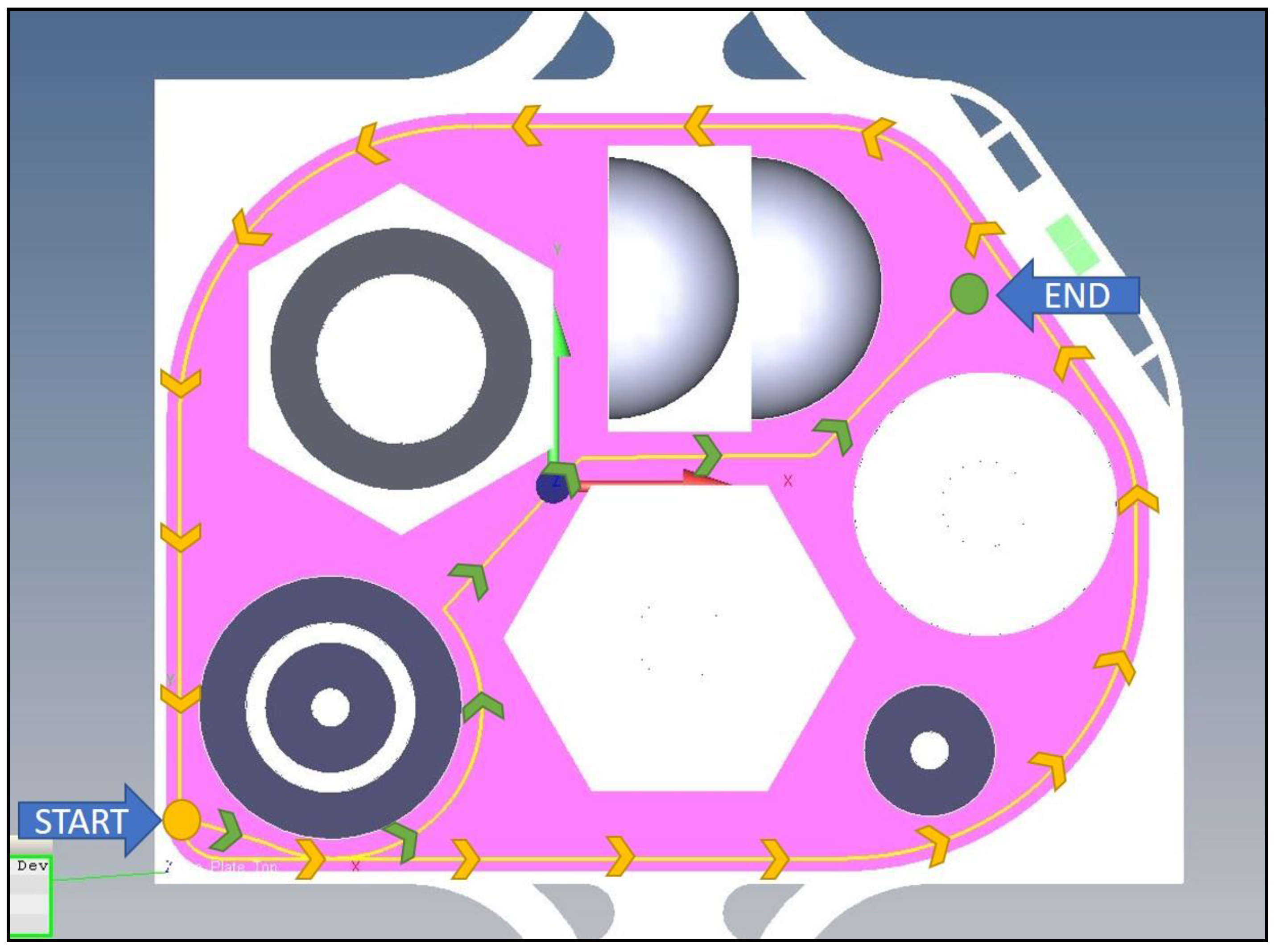
The base plate is inspected by a single path starting in the bottom left corner, moving along the edge in a counterclockwise manner, as displayed in Figure 16. When returning to the start point, the path trails off towards the interior of the specimen to make sure any warping towards the middle is included in the base alignment for, which this feature is crucial. Next, the line on HX2_Plane2 is repeated as a scanned line before the point on HX1_Plane4 concludes the CMM’s confirmation of the base alignment.
The cylinders are inspected with a helical scanning path starting at the base of convex cylinders (top of concave cylinders) at the extreme point in the x-direction, moving counterclockwise in 3 revolutions before reaching the other end, as shown in Figure 17a. The spheres are inspected by three lateral paths at 15, 45, and 75 degrees from the horizontal, as illustrated in Figure 17b, and the cones are inspected by helical paths in the same way as cylinders (Figure 17c). Finally, the planes are inspected by a continuous path, as illustrated in Figure 17d, where three square paths are connected and inspected as one.
2.5.3. Defining Characteristics
When all features are extracted and assigned an inspection strategy, the characteristics must be defined for the software to calculate the results and generate reports. The flatness of all planes in HX1 and HX2 is calculated, and a pairwise comparison is conducted to check parallelism and distance between opposing planes, i.e., plane 1 vs. plane 4, plane 2 vs. plane 5, and plane 3 vs. plane 6. For the cylinders, the cylindricity is calculated along with diameter and position. Additionally, pairwise comparison is done to check coaxiality between stacked cylinders, e.g., the convex 24 mm cylinder is compared with the 16 mm convex cylinder on top, and the convex 4 mm cylinder is compared to the 8 mm convex cylinder below it. The cones are checked for position, apex angle, and diameter at three altitudes. Unfortunately, the measurement strategy was ineffective in measuring apex angle and diameter, and the calculated results appear to be overfitted. The spherical shape features are assigned roundness characteristics along with diameter for each of the inspection paths. Moreover, a position is calculated (based on the estimated center of the sphere), and a profile characteristic is assigned. An overview is tabulated in Table 5, along with the scheme used for naming the characteristics.
2.5.4. Conducting the Inspection
The inspection is initialized from the computer, and a unique name is created for each inspection in accordance with the unique name of the specimen under consideration. All inspections are repeated three times, including the fixing and removal of the specimen from the fixture to enable the analysis of any variations that may occur from any manual operations. Even though the fixture ensures that the CMM is aware of the position of the specimen, a manual alignment is still completed at the beginning of the inspection. This because a manual alignment must be done for each specimen to account for variations between specimens, and therefore, this action should also be repeated to enable the analysis of variation arising from manual operations.
When the manual alignment is completed as described in Section 2.5.1., the CMM switches to CNC-mode and repeats the base alignment before continuing to the inspection. One repetition of the inspection took a minimum of 9 min and 20 s. Variations in elapsed time occur when deviations from nominal geometry cause the measurement to be executed with wrong measurement pressure, causing the CNC to repeat the measurement with adjusted parameters to account for the inaccuracy. This adjustment includes changing the measurement speed and thereby prolonging the inspection considerably, as outlined in Table 6. Moreover, a safety feature requires a restart of the entire inspection if the stylus collides with an obstruction. Due to the small dimensions of the smallest concave cylinder, this blind hole is difficult to properly clean and caused the inspection to fail at this shape feature multiple times. Measures were taken to secure the completion of future inspections by mechanically removing the residual powder from this hole, but this, unfortunately, renders all results from this cylinder invalid. The machine stops are not considered in Table 6 as the timer also was reset in these instances.
Every inspection is finalized by calculations of all defined features and characteristics, and a report is generated for the operator. The results are stored in a database queried by another proprietary software called PiWeb reporting that visualizes the results and offers a simple analysis of the results.
2.6. Data Analysis
This paper briefly reports on a preliminary high-level analysis whose purpose is to investigate the variation between the different blocks of the experiment. It is crucial for the validity of the experiment that the variation between the different blocks can be characterized and attributed to natural variation. This analysis is conducted in Python 3 utilizing SciPy, Numpy, and Pandas and visualized with Matplotlib and Seaborn in a Jupyter Notebook environment. The source code is available in the online repository together with the data and all relevant documentation.
The brief analysis described herein considers the results for diameter, cylindricity, and flatness. When a feature is measured by a series of points, the location of the actual surface is estimated by least-squares approximation. The diameter is hence a measure of this estimated surface, and the cylindricity is the difference between the largest positive and negative deviation from the estimated surface. Similarly, flatness is defined as the difference between the largest positive and negative deviations from the estimated plane.
3. Results
While the database contains the information on every single measurement point, the data extracted from the database are restricted to the aggregate measures defined for each characteristic, such as flatness, cylindricity, etc. All data were exported as a 257 kB comma-separated values (CSV) file for each specimen and is freely available online. The following subsections provide a brief description of the data in terms of what data are available and further perform a brief analysis of the results to characterize variation within and between a selection of variables.
3.1. Contents of CSV Files
All files are exported with the same parameters, yielding a table with the same 52 columns for all specimens, although many of these are not in use. The columns of interest are outlined in Table 7.
3.2. Variation between Repeated Measurements
The entire inspection was repeated three times for each specimen, which enables a characterization of the variation of measurements and, therefore, the reliability of measurements. The three repeated inspections were conducted in sequence and included the mounting and demounting of the specimen in the fixture, hence enabling the analysis of this variation in the study. In addition to the natural random variations of the measurement setup, the experiment is also prone to variations arising from the minuscule deviations from one mounting in the CMM to the next, effectively offsetting the inspection path. Figure 18 plots the three repeated inspections of HX1_Plane1 from specimen #6 from build 3 (Build3_#6_HX1_Plane1). Some minor variations are apparent in the figure, and even though the measured surface topology is close to identical, the minor deviations give rise to the three measured error values 0.062, 0.058, and 0.059 mm, respectively.
The preliminary analysis indicates that there is indeed some variation between repeated measurements as introduced in Figure 18 and further detailed in Table 8. This preliminary analysis considers the measurements of cylindricity, diameter, and flatness of all the relevant features except for the 4mm concave cylinder omitted due to residual powder not removable by pressurized air. With 7 cylindricity-, 7 diameter- and 12 flatness measurements for all 135 specimens, we obtain a total of 3510 data points for each repeated inspection. To analyze the variation between measurements, we compute the mean value of the three repeated measurements and—more importantly—the difference between the highest and the lowest value among the repeated measurements (∆). The characteristics of this data set are described in Table 8, where Rep 1–3 corresponds to the measured error of the first, second and third repeated inspections, respectively, Rep Mean is the mean value of the three repeated measurements and ∆ is the difference between the highest and lowest measured error. The negative values originate from deviations where the measured diameters are smaller than the nominal values. Form errors (i.e., cylindricity and flatness) may only take positive values since this is the distance between the most extreme positive and negative deviations from a perfect geometry.
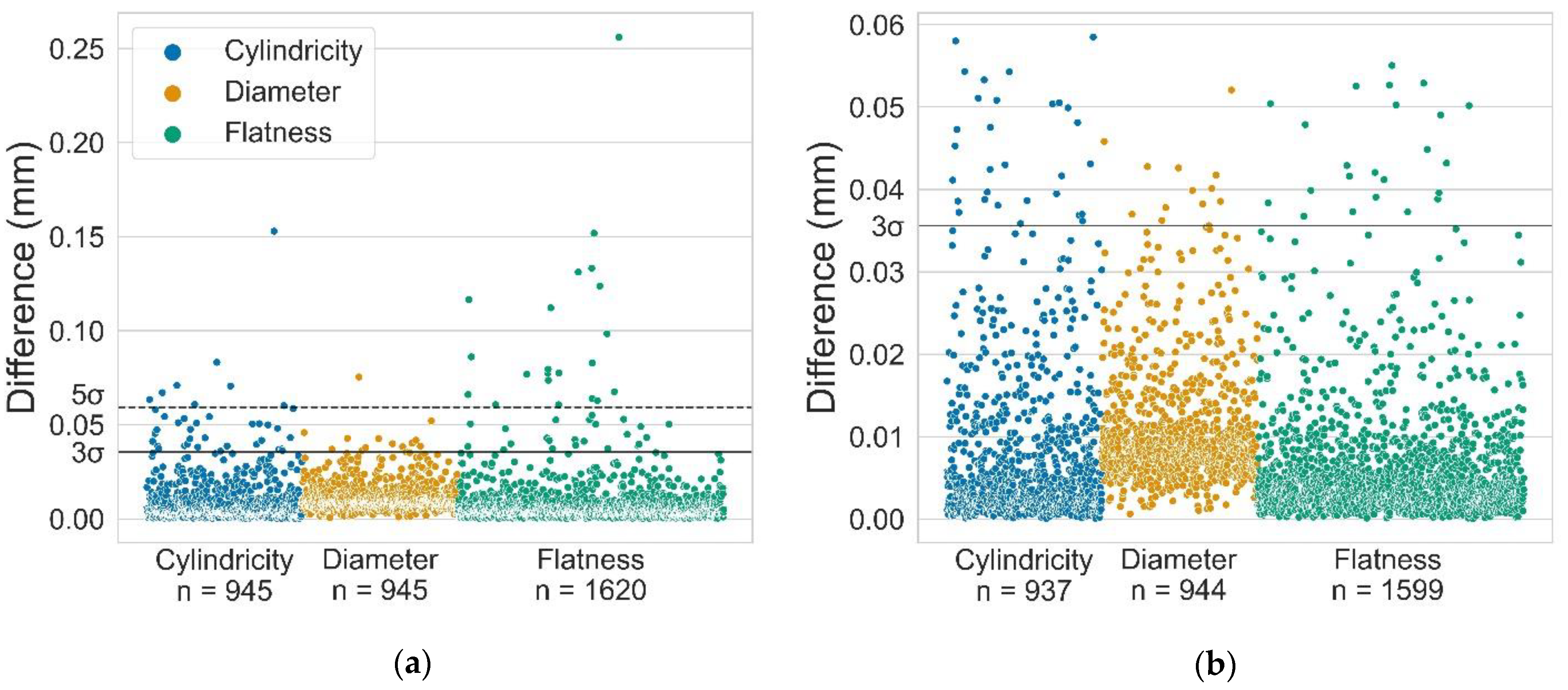
Table 8 reveals a general declining trend in measured error through the repeated inspections, which can be explained by the removal of some residual powder during and between the inspections. This effect may be amplified by the fact that the probe is following the same path and might leave a trail or a slight indentation on the surface. Figure 19 contains a scatterplot where ∆ is plotted for the different characteristics, and outliers are clearly visible. These outliers contribute to a higher variance, which makes unfiltered data difficult to analyze graphically; hence, Figure 19b only includes the data points below five standard deviations (5σ). The width of the groups reflects the number of points.
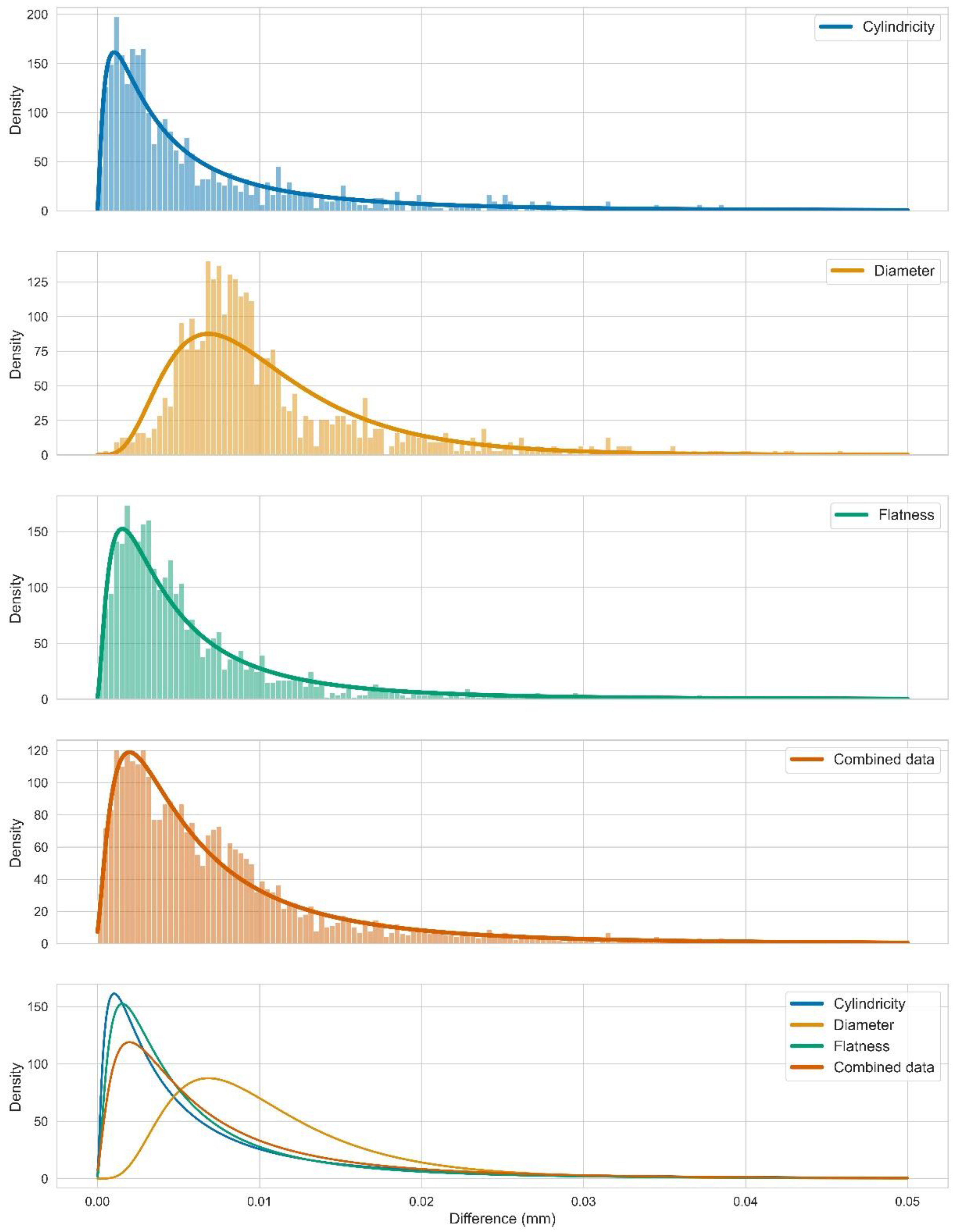
The plots of Figure 19 show a high-density of points close to zero, which indicates that the observed variations do not follow a normal distribution but rather a lognormal distribution where a higher density is observed close to zero. Figure 20 briefly explores this observation by fitting a lognormal distribution to the data and comparing this to normalized histograms of the distributions. These plots do indeed indicate that the distribution roughly follows a lognormal distribution where the measurements of diameter stand out as slightly less repeatable compared to the distributions of flatness and cylindricity. This discrepancy may be explained by the diameter being estimated by the least-squares method and hence consider all the measured values, while the geometric errors of flatness and cylindricity are solely dependent on the extremes of the measured points.
3.3. Variation between Builds
The build layout of the experiment enables the comparison of the different builds by inspecting the anchor specimens, which are in the exact same position and orientation for every build. Furthermore, another possibility to compare the builds is provided by the geometry of the artifact and the fact that all specimens are rotated about a single axis, effectively leaving Planes 2 and 5 of HX2 vertical for all orientations. This means that there are comparable data points available for all positions in the build space for all three builds.
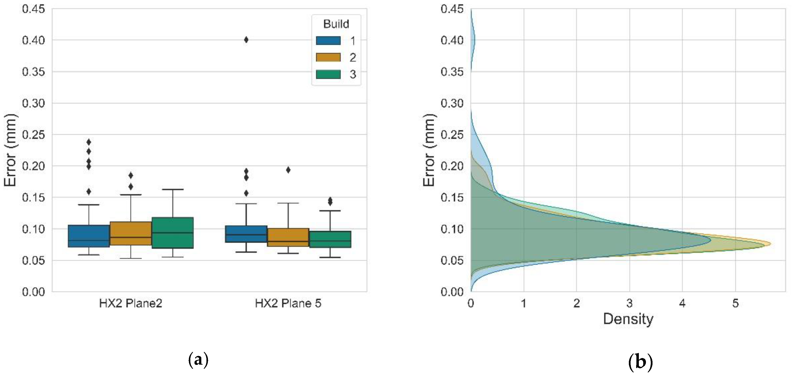
Figure 21 display the variation between the three builds when considering the mean value of the three repeated measurements for the vertical planes in all locations in the build space. While some variations are present, the data appears to be quite consistent between builds, with a few outliers disrupting the homogeneity of the distributions. The kernel density estimation of Figure 21b indicates quite similar distributions between the three builds, again with some influence from outliers. A statistical description is presented in Table 9 for both planes, where the difference is the difference between the minimum and maximum measured flatness error of a plane in the same position in the three builds.
3.4. Variation between Positions in the Build Chamber
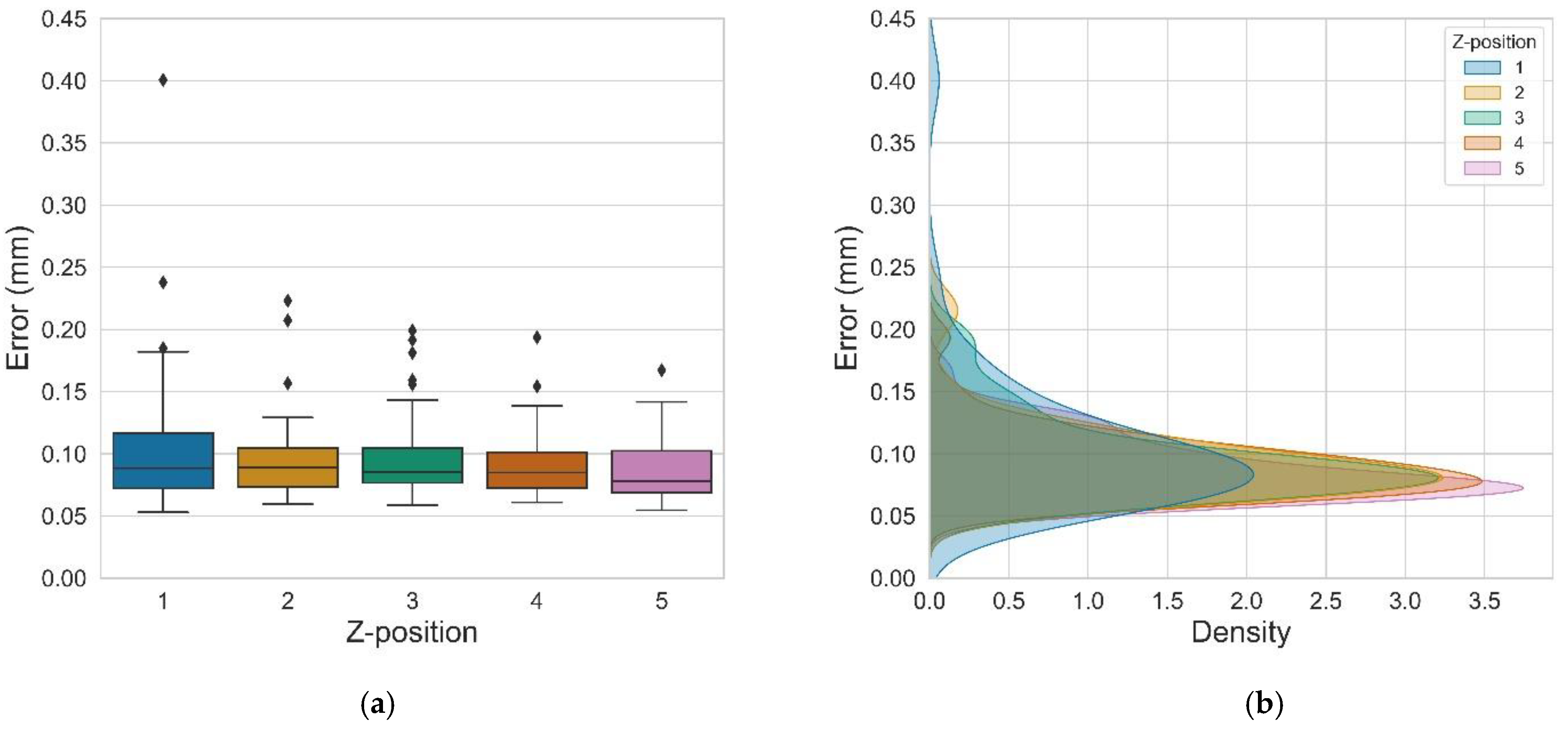
The designed build layout facilitates the comparison of discrete positions in the build chamber in the z-direction as well as in the xy-plane. A slight trend towards tighter tolerances in the higher end of the build may be observed in Figure 22a, but the statistical significance of this trend is inconclusive from the current analysis. Except for one extreme outlier at the lowest level, the distributions among the different z-levels are quite similar, as seen in the kernel density estimation of Figure 22b. The statistical description of the data is tabulated in Table 10, where the columns correspond to the five levels of z-positions, the mean value for all z-levels of a specific position considered across all three builds, and the difference is calculated as the difference between the minimum and the maximum value from the same population.
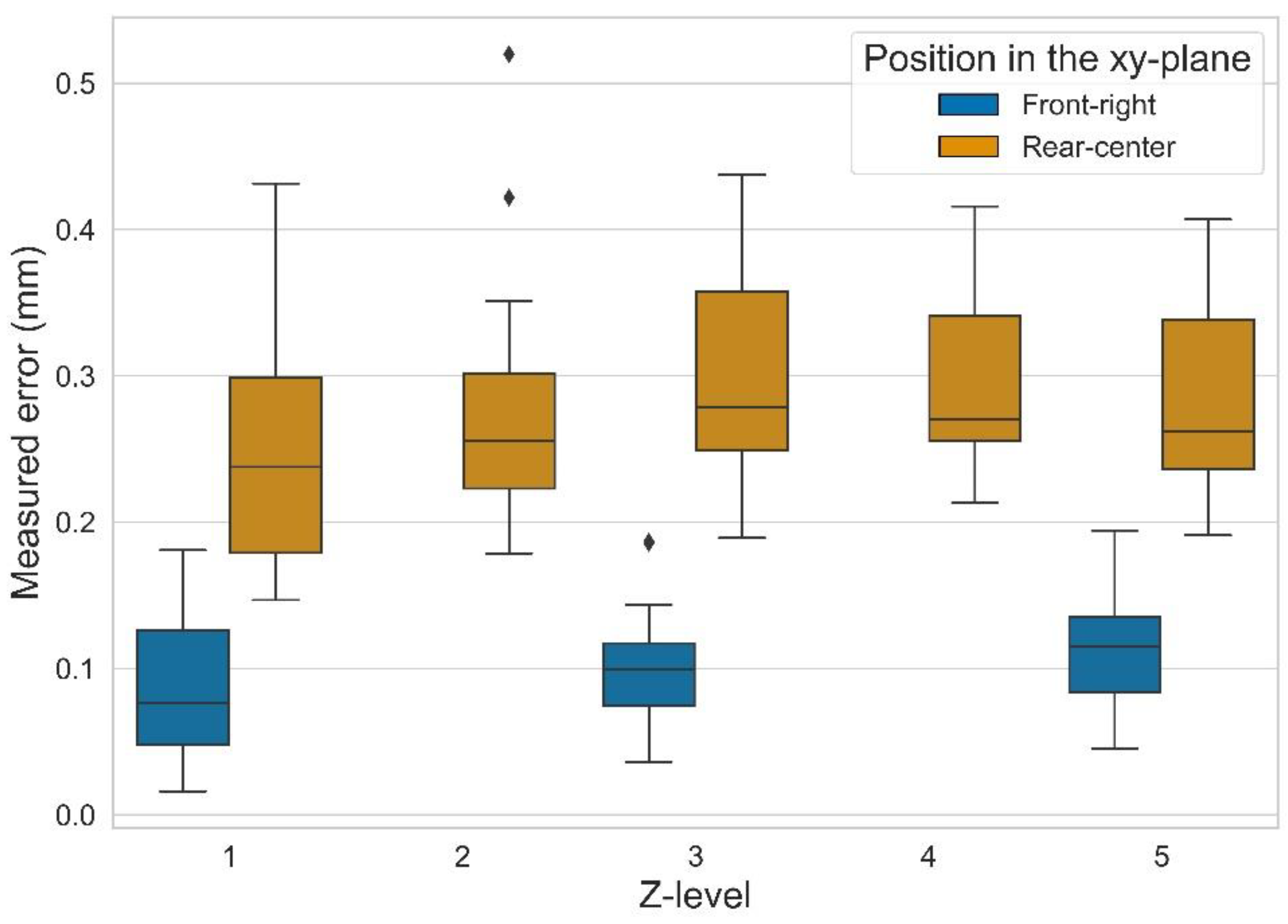
A more distinct variation may be found within each z-level as the position in the xy-plane appears to be of significant influence on the geometric accuracy and the observed variation. This discrepancy is apparent in all the preliminary analyses but exemplified here by diametrical error due to the clear results for this particular characteristic. When comparing the diametrical error of cylinders fabricated in the front-right corner to the ones fabricated at the rear center, it is clear that the position in the front-right is far more accurate than the rear positions, as shown in Figure 23.
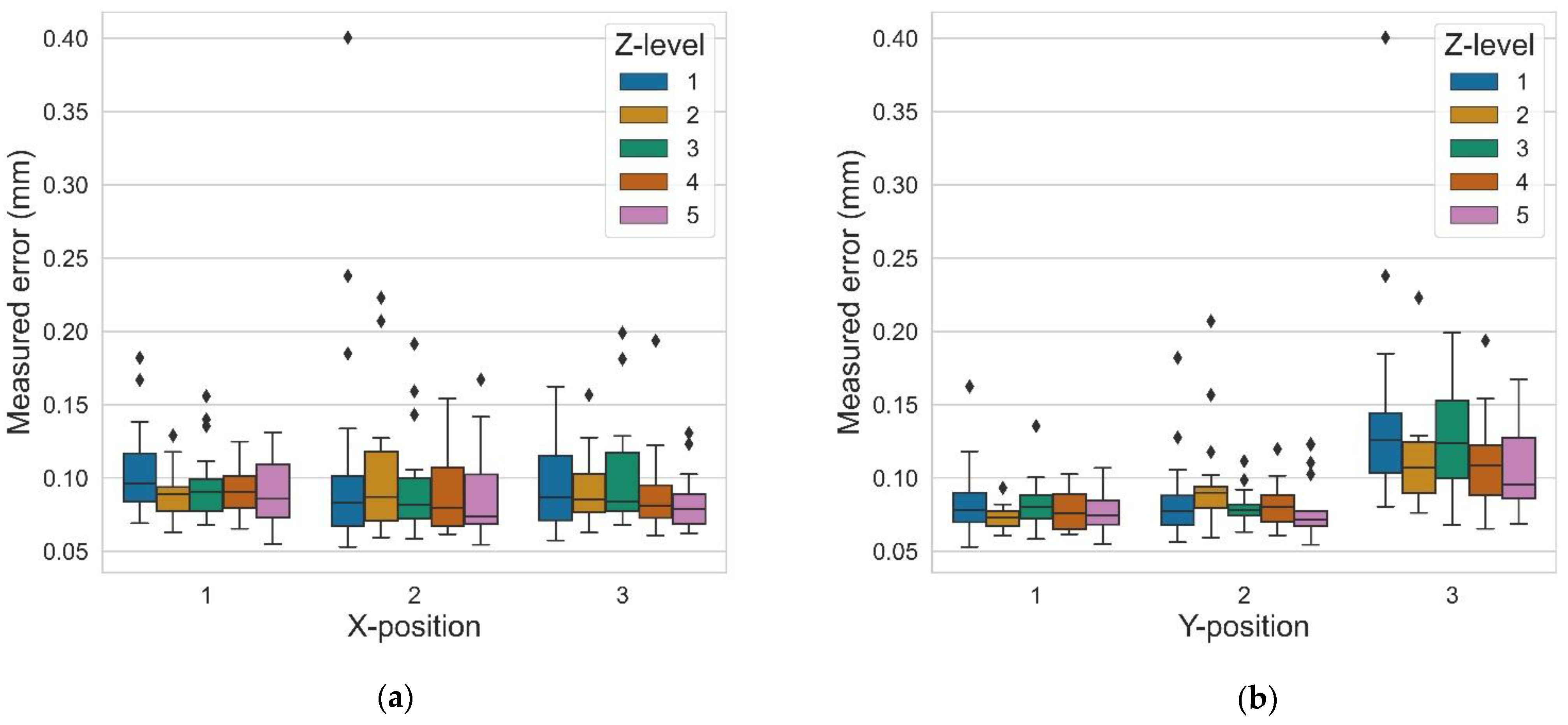
Recall that the anchor specimens are only fabricated in the front-right position at layers 1, 3, and 5, hence the gaps in the above observation. A more holistic analysis may be conducted by comparing the vertical planes, i.e., planes 2 and 5 of HX2, which enables the comparison of all positions in the build space. The boxplot of Figure 24 shows the measured variations considering the specimens’ position along the x- and y-axes. While Figure 24a displays quite uniform distribution between the three rows in the x-direction, Figure 24b exhibits a rather clear discrepancy in the third position, i.e., the rear of the build chamber.
4. Discussion
The described experiment is designed, planned, and executed to produce repeatable and valid results. By developing a rigid methodology and performing automated data acquisition with a CMM, the obtained data should be of high-quality. At present, however, there are many unknown factors and even a couple of minor discrepancies discovered in the analysis. The following subsections contain declarations of the known discrepancies, as well as the known unknowns, accompanied by a short discussion of the possible consequences of these factors. Finally, a discussion is made on the implications of underlying assumptions and the scope of the current study with possible directions for further work.
4.1. Hitherto Discovered Discrepancies
At the time of publication, all discovered discrepancies are considered minor inconveniences with marginal effect on the validity of the current study. The most noteworthy deviation from the original plan is the issues related to the smallest concave cylinder (CC2), where the residual powder was difficult to remove due to the blind hole. Because the CMM inspection was impaired, the scan strategy for this particular feature was altered, and the remaining powder was removed mechanically effectively, rendering all results related to this feature invalid, including the roundness, cylindricity, and position of this feature as well as its relation to other features (i.e., coaxiality). The problem of residual powder is omnipresent in LB-PBF/P partly due to the material being prone to static electricity, which impedes the proper removal of powder. This study aims at investigating the as-build geometry and, therefore, avoided mechanical removal of powder, which could mitigate the problem of adhering particles but could also damage the surface and obscure the results.
Although a full analysis of the collected data has not yet been conducted, potential issues were observed during the inspections related to cones and spheres as the calculated diameter and apex angle were identical to nominal values. This is obviously not the reality and probably a result of inappropriate inspection strategies and evaluation methods for the features in question. Consequently, the use of these measurements should be used with extra care but does not affect the overall inspection in any way.
Additional discrepancies are limited to naming errors where corner specimens of the third build are labeled as build 1, and inspection results for select characteristics are labeled incorrectly. The mislabeling of the corner specimens has a marginal impact as this error was detected during postprocessing, and the specimens from the three builds are kept separate, thus preventing cross-contamination. Naming errors from the inspections of the main specimens are limited to typographical errors, which may cause some issues in automatic data processing but are easily handled in data preparation when they are known in advance. These naming errors are explicitly disclosed in the online repository.
4.2. External Factors
All experiments are subject to external factors that cannot be controlled. One such factor is the weather conditions that influence the experiment, especially in terms of humidity, which may influence the powder during sintering. Moreover, while the AM machine is situated in a room with thorough climate control, the CMM and the areas between are not subject to the same level of control. Hence, the specimens were stored in the areas of climate control and transported to the CMM in batches to minimize exposure to uncontrolled environments. Weather data for the relevant days are available in the online repository.
Due to restricted access to build parameters, the “Balanced” profile was chosen for the machine settings of the EOSINT P395, which is assumed to constitute a reasonable tradeoff between accuracy and speed. Note that finer settings are available, which could yield more accurate results than what is reported in the present study. However, the goal is not to achieve the best possible results but rather to investigate the influence of other factors (e.g., part build orientation); hence keeping the machine settings constant is sufficient to fulfill the purpose of this study without compromising its validity.
4.3. Implications of Assumptions and Boundaries
The current work assumes that the utilized technologies are able to fabricate and detect the targeted deviations with sufficient accuracy to yield valid results. This is especially relevant for the choice of probe size for the CMM, which acts as a filter for the surface roughness [40]. A probe diameter of 3 mm was selected not only for practical reasons but also to facilitate the analysis of geometric deviation without the noise imposed by surface roughness. A smaller probe could enable the analysis of narrow grooves, thus potentially exposing additional surface variations and defects, while the filtering could still be conducted numerically to enable an analysis of larger variations. Such inspections and analyses could be compared to the collected data but are—for now—left for future work.
The present study was limited to external geometric and dimensional accuracy where the CMM was the measuring instrument of choice. Investigations of surface roughness, mechanical properties, and internal structures are outside the scope of this study and are left for future work. While these areas are the subject of many research efforts, the preliminary results of the current study, as well as results of related research, suggest that the variations between positions in the build space are substantial and cannot be neglected in the design of experiments for LB-PBF/P. Closer examination of these effects in other AM technologies constitutes an avenue of future research—first of all for LB-PBF/M, but perhaps also other powder bed systems.
5. Conclusions
This paper described the design and execution of an elaborate experiment to generate valid and reproducible data on dimensional and geometric accuracy in LB-PBF/P. The following conclusions can be drawn from the analysis:
- The experiment design described herein enabled the analysis and characterization of variation between the different builds and between various positions in the build chamber;
- The variation between the builds appears to be negligible, and the three builds can be compared without loss of validity;
- There is a slight trend of higher accuracy towards the higher levels of the builds (higher z-coordinates), but this trend is not found to be statistically significant;
- The variation in the xy-plane is significant, with considerably larger geometric and dimensional errors towards the rear of the machine. No efforts are made to explain this discrepancy.
The current research warrants further investigations into variation management in LB-PBF and especially the control of noise factors to ensure valid and reliable results in future experiments. The analysis presented in the current paper is merely scraping the surface of the data generated from the experiment, and thorough analysis is left for future work. Moreover, the data enables the development of numerical models for the prediction of geometric and dimensional accuracy. The next step of the current project involves further analysis of the data to construct predictive models for geometric and dimensional accuracy. The additional specimens produced through the described experiment have not been inspected and, therefore, constitute a major source of unrevealed data that can be utilized to further improve the understanding of LB-PBF/P.
Author Contributions
Conceptualization, T.L.L., and O.S.; methodology, T.L.L., and O.S.; formal analysis, T.L.L.; investigation, T.L.L.; data curation, T.L.L.; writing—original draft preparation, T.L.L.; writing—review and editing, O.S.; visualization, T.L.L.; supervision, O.S.; project administration, T.L.L. All authors have read and agreed to the published version of the manuscript.
Funding
This research is funded by the Norwegian Ministry of Research and Education through the PhD-scholarship of Torbjørn Langedahl Leirmo.
Institutional Review Board Statement
Not applicable.
Informed Consent Statement
Not applicable.
Data Availability Statement
Data, artifacts, and all code for analysis are available online through a repository at GitHub: https://github.com/TheThorb/Leirmo_Exp1_Publication1.
Acknowledgments
The authors would like to acknowledge the contributions of Ivanna Baturynska in the planning of the experiment and Pål Erik Endrerud for facilitating the experiment execution.
Conflicts of Interest
The authors declare no conflict of interest.
Abbreviations
| 3D | Three dimensional |
| AM | Additive manufacturing |
| ASCII | American Standard Code for Information Interchange |
| CAD | Computer-aided design |
| CMM | Coordinate measuring machine |
| CNC | Computer numerical control |
| CSV | Comma-separated values |
| FFF | Fused-filament fabrication |
| GD&T | Geometric dimensioning and tolerancing |
| GPS | Geometric product specifications |
| LB-PBF | Laser-based powder bed fusion |
| LB-PBF/M | Laser-based powder bed fusion of metals |
| LB-PBF/P | Laser-based powder bed fusion of polymers |
| PA12 | Polyamide 12 |
| PBF | Powder bed fusion |
| PLA | Polylactic acid |
| SLS | Selective laser sintering |
| STEP | Standard for the exchange of product model data |
| STL | Stereolithography (file format) |
Appendix A

Table A1.
Overview of all defined positions in the build space and the orientation fabricated in each position and for each build. The anchor positions are highlighted for clarity.
Table A1.
Overview of all defined positions in the build space and the orientation fabricated in each position and for each build. The anchor positions are highlighted for clarity.
| Position | Rotation about x-Axis (Degrees) | ||||||||
|---|---|---|---|---|---|---|---|---|---|
| Index | Relative | Center Point (mm) | Build 1 | Build 2 | Build 3 | ||||
| x | y | z | x | y | z | ||||
| 1 | 1 | 1 | 1 | 70 | 70 | 50.88 | 70 | 70 | 70 |
| 2 | 2 | 1 | 1 | 170 | 70 | 50.88 | 140 | 140 | 140 |
| 3 | 3 | 1 | 1 | 270 | 70 | 50.88 | −90 | −90 | −90 |
| 4 | 1 | 2 | 1 | 70 | 170 | 50.88 | 145 | 145 | 145 |
| 5 | 2 | 2 | 1 | 170 | 170 | 50.88 | 165 | 165 | 165 |
| 6 | 3 | 2 | 1 | 270 | 170 | 50.88 | 120 | 120 | 120 |
| 7 | 1 | 3 | 1 | 70 | 270 | 50.88 | 110 | 110 | 110 |
| 8 | 2 | 3 | 1 | 170 | 270 | 50.88 | −90 | −90 | −90 |
| 9 | 3 | 3 | 1 | 270 | 270 | 50.88 | 35 | 35 | 35 |
| 10 | 1 | 1 | 2 | 70 | 70 | 150.6 | 70 | 70 | 70 |
| 11 | 2 | 1 | 2 | 170 | 70 | 150.6 | 140 | 140 | 140 |
| 12 | 3 | 1 | 2 | 270 | 70 | 150.6 | −90 | −90 | −90 |
| 13 | 1 | 2 | 2 | 70 | 170 | 150.6 | 145 | 145 | 145 |
| 14 | 2 | 2 | 2 | 170 | 170 | 150.6 | 165 | 165 | 165 |
| 15 | 3 | 2 | 2 | 270 | 170 | 150.6 | 120 | 120 | 120 |
| 16 | 1 | 3 | 2 | 70 | 270 | 150.6 | 110 | 110 | 110 |
| 17 | 2 | 3 | 2 | 170 | 270 | 150.6 | −90 | −90 | −90 |
| 18 | 3 | 3 | 2 | 270 | 270 | 150.6 | 35 | 35 | 35 |
| 19 | 1 | 1 | 3 | 70 | 70 | 250.32 | 70 | 70 | 70 |
| 20 | 2 | 1 | 3 | 170 | 70 | 250.32 | 140 | 140 | 140 |
| 21 | 3 | 1 | 3 | 270 | 70 | 250.32 | −90 | −90 | −90 |
| 22 | 1 | 2 | 3 | 70 | 170 | 250.32 | 145 | 145 | 145 |
| 23 | 2 | 2 | 3 | 170 | 170 | 250.32 | 165 | 165 | 165 |
| 24 | 3 | 2 | 3 | 270 | 170 | 250.32 | 120 | 120 | 120 |
| 25 | 1 | 3 | 3 | 70 | 270 | 250.32 | 110 | 110 | 110 |
| 26 | 2 | 3 | 3 | 170 | 270 | 250.32 | −90 | −90 | −90 |
| 27 | 3 | 3 | 3 | 270 | 270 | 250.32 | 35 | 35 | 35 |
| 28 | 1 | 1 | 4 | 70 | 70 | 350.04 | 70 | 70 | 70 |
| 29 | 2 | 1 | 4 | 170 | 70 | 350.04 | 140 | 140 | 140 |
| 30 | 3 | 1 | 4 | 270 | 70 | 350.04 | −90 | −90 | −90 |
| 31 | 1 | 2 | 4 | 70 | 170 | 350.04 | 145 | 145 | 145 |
| 32 | 2 | 2 | 4 | 170 | 170 | 350.04 | 165 | 165 | 165 |
| 33 | 3 | 2 | 4 | 270 | 170 | 350.04 | 120 | 120 | 120 |
| 34 | 1 | 3 | 4 | 70 | 270 | 350.04 | 110 | 110 | 110 |
| 35 | 2 | 3 | 4 | 170 | 270 | 350.04 | −90 | −90 | −90 |
| 36 | 3 | 3 | 4 | 270 | 270 | 350.04 | 35 | 35 | 35 |
| 37 | 1 | 1 | 5 | 70 | 70 | 449.76 | 70 | 70 | 70 |
| 38 | 2 | 1 | 5 | 170 | 70 | 449.76 | 140 | 140 | 140 |
| 39 | 3 | 1 | 5 | 270 | 70 | 449.76 | −90 | −90 | −90 |
| 40 | 1 | 2 | 5 | 70 | 170 | 449.76 | 145 | 145 | 145 |
| 41 | 2 | 2 | 5 | 170 | 170 | 449.76 | 165 | 165 | 165 |
| 42 | 3 | 2 | 5 | 270 | 170 | 449.76 | 120 | 120 | 120 |
| 43 | 1 | 3 | 5 | 70 | 270 | 449.76 | 110 | 110 | 110 |
| 44 | 2 | 3 | 5 | 170 | 270 | 449.76 | −90 | −90 | −90 |
| 45 | 3 | 3 | 5 | 270 | 270 | 449.76 | 35 | 35 | 35 |
References
- Wohlers Associates Inc. Wohlers Report 2019; Wohlers Associates Inc.: Fort Collins, CO, USA, 2019. [Google Scholar]
- ISO 1101:2017(E). Geometrical Product Specifications (GPS)—Geometrical Tolerancing—Tolerances of Form, Orientation, Location And Run-Out; International Organization for Standardization: Geneva, Switzerland, 2017. [Google Scholar]
- ASME Y14.5M-2018. Dimensioning and Tolerancing; ASME: New York, NY, USA, 2018. [Google Scholar]
- ISO/ASTM 52900:2015(E). Standard Terminology for Additive Manufacturing—General Principles—Terminology; ISO/ASTM: West Conshohocken, PA, USA, 2015. [Google Scholar]
- ISO/ASTM 52911:2019(E). Additive Manufacturing—Design—Part 2: Laser-Based Powder Bed Fusion of Polymers; ISO/ASTM: Geneva, Switzerland, 2019. [Google Scholar]
- Delfs, P.; Tows, M.; Schmid, H.J. Optimized build orientation of additive manufactured parts for improved surface quality and build time. Addit. Manuf. 2016, 12, 314–320. [Google Scholar] [CrossRef]
- Arni, R.; Gupta, S.K. Manufacturability analysis of flatness tolerances in solid freeform fabrication. J. Mech. Des. 2001, 123, 148–156. [Google Scholar] [CrossRef]
- Paul, R.; Anand, S. Optimal part orientation in Rapid Manufacturing process for achieving geometric tolerances. J. Manuf. Syst. 2011, 30, 214–222. [Google Scholar] [CrossRef]
- Zhang, Y.; Bernard, A.; Gupta, R.K.; Harik, R. Feature based building orientation optimization for additive manufacturing. Rapid Prototyp. J. 2016, 22, 358–376. [Google Scholar] [CrossRef]
- Cheng, W.; Fuh, J.Y.H.; Nee, A.Y.C.; Wong, Y.S.; Loh, H.T.; Miyazawa, T. Multi-objective optimization of part-building orientation in stereolithography. Rapid Prototyp. J. 1995, 1, 12–23. [Google Scholar] [CrossRef]
- Salmoria, G.V.; Leite, J.L.; Vieira, L.F.; Pires, A.T.N.; Roesler, C.R.M. Mechanical properties of PA6/PA12 blend specimens prepared by selective laser sintering. Polym. Test. 2012, 31, 411–416. [Google Scholar] [CrossRef] [Green Version]
- Caulfield, B.; McHugh, P.E.; Lohfeld, S. Dependence of mechanical properties of polyamide components on build parameters in the SLS process. J. Mater. Process. Technol. 2007, 182, 477–488. [Google Scholar] [CrossRef]
- Baturynska, I. Application of Machine Learning Techniques to Predict the Mechanical Properties of Polyamide 2200 (PA12) in Additive Manufacturing. Appl. Sci. 2019, 9, 1060. [Google Scholar] [CrossRef] [Green Version]
- Beitz, S.; Uerlich, R.; Bokelmann, T.; Diener, A.; Vietor, T.; Kwade, A. Influence of Powder Deposition on Powder Bed and Specimen Properties. Materials 2019, 12, 297. [Google Scholar] [CrossRef] [PubMed] [Green Version]
- Pavan, M.; Faes, M.; Strobbe, D.; Van Hooreweder, B.; Craeghs, T.; Moens, D.; Dewulf, W. On the influence of inter-layer time and energy density on selected critical-to-quality properties of PA12 parts produced via laser sintering. Polym. Test. 2017, 61, 386–395. [Google Scholar] [CrossRef]
- Kundera, C.; Kozior, T. Evaluation of the influence of selected parameters of Selective Laser Sintering technology on surface topography. J. Phys. Conf. Ser. 2019, 1183, 012002. [Google Scholar] [CrossRef]
- Sachdeva, A.; Singh, S.; Sharma, V.S. Investigating surface roughness of parts produced by SLS process. Int. J. Adv. Manuf. Technol. 2013, 64, 1505–1516. [Google Scholar] [CrossRef]
- Mavoori, N.K.; Vekatesh, S.; M, M.H. Investigation on surface roughness of sintered PA2200 prototypes using Taguchi method. Rapid Prototyp. J. 2018, 25, 454–461. [Google Scholar] [CrossRef]
- Reinhardt, T.; Martha, A.; Witt, G.; Köhler, P. Preprocess-Optimization for Polypropylene Laser Sintered Parts. Comput.-Aided Des. Appl. 2014, 11, 49–61. [Google Scholar] [CrossRef]
- Pavan, M. CT-Based Optimization of Laser Sintering of Polyamide-12; KU Leuven: Brussels, Belgium, 2018. [Google Scholar]
- Baturynska, I. Statistical analysis of dimensional accuracy in additive manufacturing considering STL model properties. Int. J. Adv. Manuf. Technol. 2018, 2835–2849. [Google Scholar] [CrossRef]
- Ha, S.; Ransikarbum, K.; Han, H.; Kwon, D.; Kim, H.; Kim, N. A dimensional compensation algorithm for vertical bending deformation of 3D printed parts in selective laser sintering. Rapid Prototyp. J. 2018, 24, 955–963. [Google Scholar] [CrossRef]
- Di Angelo, L.; Di Stefano, P.; Guardiani, E. Search for the Optimal Build Direction in Additive Manufacturing Technologies: A Review. J. Manuf. Mater. Process. 2020, 4, 71. [Google Scholar] [CrossRef]
- Taufik, M.; Jain, P.K. Role of build orientation in layered manufacturing: A review. Int. J. Manuf. Technol. Manag. 2013, 27, 47–73. [Google Scholar] [CrossRef]
- Senthilkumaran, K.; Pandey, P.M.; Rao, P.V.M. Statistical modeling and minimization of form error in SLS prototyping. Rapid Prototyp. J. 2012, 18, 38–48. [Google Scholar] [CrossRef]
- Sood, A.K.; Ohdar, R.K.; Mahapatra, S.S. Improving dimensional accuracy of Fused Deposition Modelling processed part using grey Taguchi method. Mater. Des. 2009, 30, 4243–4252. [Google Scholar] [CrossRef]
- Rizzuti, S.; De Napoli, L.; Ventra, S. The Influence of Build Orientation on the Flatness Error in Artifact Produced by Direct Metal Laser Sintering (DMLS) Process. In Proceedings of the International Joint Conference on Mechanics, Design Engineering & Advanced Manufacturing, Cham, Switzerland, 14–16 September 2019; pp. 463–472. [Google Scholar]
- Nidagundi, V.B.; Keshavamurthy, R.; Prakash, C.P.S. Studies on Parametric Optimization for Fused Deposition Modelling Process. Mater. Today: Proc. 2015, 2, 1691–1699. [Google Scholar] [CrossRef]
- Ollison, T.; Berisso, K. Three-Dimensional Printing Build Variables That Impact Cylindricity. J. Ind. Technol. 2010, 26, 2–10. [Google Scholar]
- Minetola, P.; Calignano, F.; Galati, M. Comparing geometric tolerance capabilities of additive manufacturing systems for polymers. Addit. Manuf. 2020, 32, 101103. [Google Scholar] [CrossRef]
- Fahad, M.; Hopkinson, N. Evaluation and comparison of geometrical accuracy of parts produced by sintering-based additive manufacturing processes. Int. J. Adv. Manuf. Technol. 2017, 88, 3389–3394. [Google Scholar] [CrossRef]
- Brøtan, V. A new method for determining and improving the accuracy of a powder bed additive manufacturing machine. Int. J. Adv. Manuf. Technol. 2014, 74, 1187–1195. [Google Scholar] [CrossRef]
- Rebaioli, L.; Fassi, I. A review on benchmark artifacts for evaluating the geometrical performance of additive manufacturing processes. Int. J. Adv. Manuf. Technol. 2017, 93, 2571–2598. [Google Scholar] [CrossRef]
- Minetola, P.; Iuliano, L.; Marchiandi, G. Benchmarking of FDM Machines through Part Quality Using IT Grades. Procedia Cirp. 2016, 41, 1027–1032. [Google Scholar] [CrossRef] [Green Version]
- Szilvśi-Nagy, M.; Mátyási, G. Analysis of STL files. Math. Comput. Model. 2003, 38, 945–960. [Google Scholar] [CrossRef]
- Leirmo, T.L.; Semeniuta, O.; Martinsen, K. Tolerancing from STL data: A Legacy Challenge. Procedia Cirp. 2020, 92, 218–223. [Google Scholar] [CrossRef]
- ISO/ASTM 52921:2013(E). Standard Terminology for Additive Manufacturing—Coordinate Systems and Test Methodologies; ISO/ASTM: Geneva, Switzerland, 2013. [Google Scholar]
- ISO/ASTM 52902:2019(E). Additive Manufacturing—Test Artifacts—Geometric Capability Assessment of Additive Manufacturing Systems; ISO/ASTM: Geneva, Switzerland, 2019. [Google Scholar]
- Rott, S.; Ladewig, A.; Friedberger, K.; Casper, J.; Full, M.; Schleifenbaum, J.H. Surface roughness in laser powder bed fusion—Interdependency of surface orientation and laser incidence. Addit. Manuf. 2020, 36, 101437. [Google Scholar] [CrossRef]
- Lou, S.; Brown, S.B.; Sun, W.; Zeng, W.; Jiang, X.; Scott, P.J. An investigation of the mechanical filtering effect of tactile CMM in the measurement of additively manufactured parts. Measurement 2019, 144, 173–182. [Google Scholar] [CrossRef]
Figure 1.
Process categories in additive manufacturing as defined in ISO/ASTM 52900:2015 and 52911:2019.
Figure 1.
Process categories in additive manufacturing as defined in ISO/ASTM 52900:2015 and 52911:2019.

Figure 2.
The test artifact designed for the experiment. (a) The computer-aided design (CAD) model with labeled features in perspective; (b) top view of the CAD model showing the numbering of planes in HX1 and HX2.
Figure 2.
The test artifact designed for the experiment. (a) The computer-aided design (CAD) model with labeled features in perspective; (b) top view of the CAD model showing the numbering of planes in HX1 and HX2.

Figure 3.
The first step of build space segmentation. (a) The build space as seen from the top; (b) the build space as seen from the front of the machine.
Figure 3.
The first step of build space segmentation. (a) The build space as seen from the top; (b) the build space as seen from the front of the machine.

Figure 4.
Numbered positions for the specimens and the positions of the “anchor” specimens. (a) The bottom layer of specimens numbered 1 through 9. Position 3 is reserved anchor specimens for z-layers 1, 3, and 5, while position 8 is reserved anchor specimens for all z-layers; (b) a front view showing the first three numbers of each layer (the front row).

Figure 5.
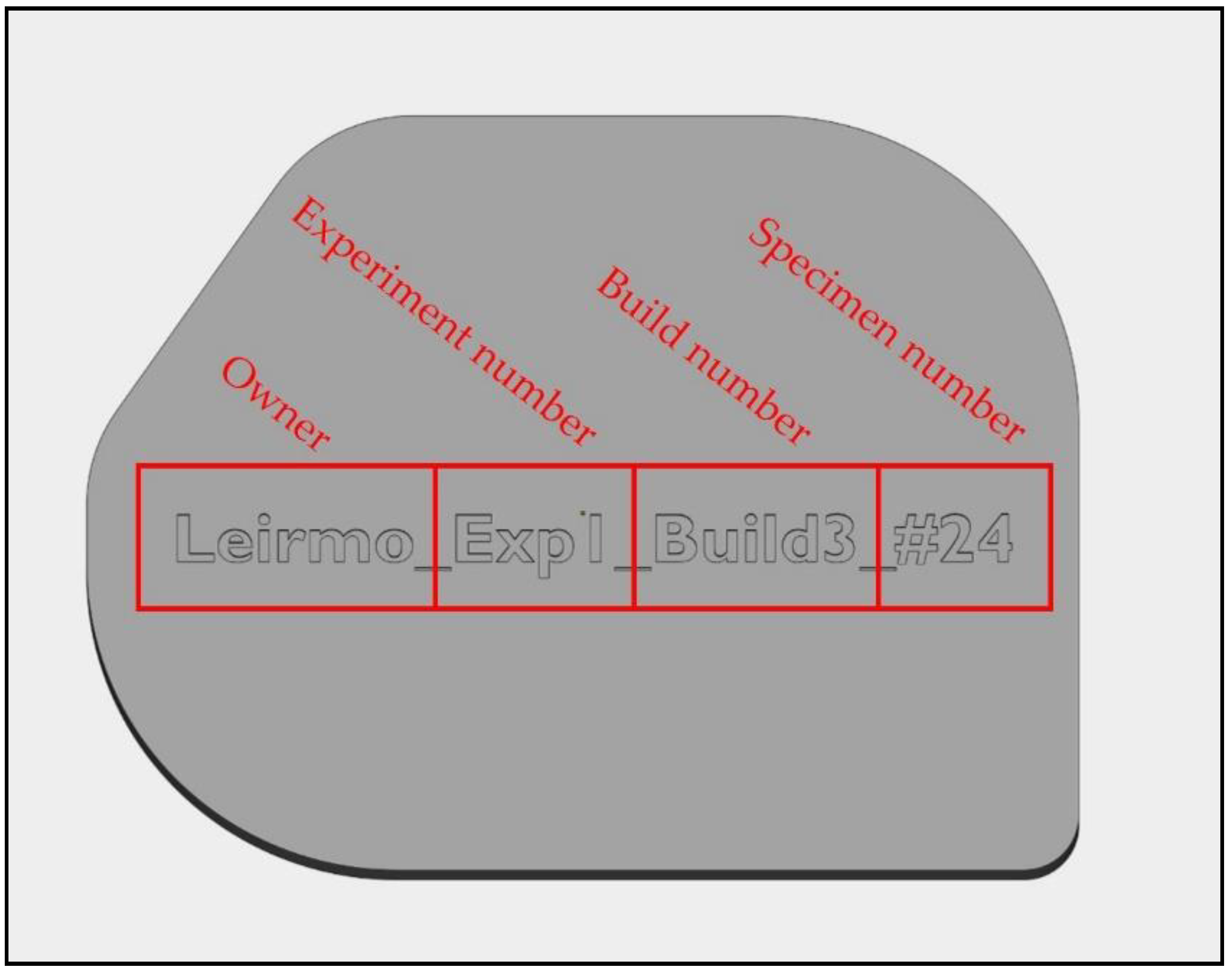
Illustration of the labeling scheme applied in the experiment. The writing is imprinted and embedded in the stereolithography (STL) file during layout preparation in Magics 23.01.
Figure 5.
Illustration of the labeling scheme applied in the experiment. The writing is imprinted and embedded in the stereolithography (STL) file during layout preparation in Magics 23.01.

Figure 6.
Slice distribution graphs showing the sintered area per layer. (a) Slice distribution for build 1 without additional specimens; (b) slice distribution for perfect spheres of 90 mm diameter in all positions.
Figure 6.
Slice distribution graphs showing the sintered area per layer. (a) Slice distribution for build 1 without additional specimens; (b) slice distribution for perfect spheres of 90 mm diameter in all positions.

Figure 7.
Open volumes available to even out the slice distribution. (a) Top view of available spaces in the xy-plane; (b) front view of the available spaces along the z-axis.
Figure 7.
Open volumes available to even out the slice distribution. (a) Top view of available spaces in the xy-plane; (b) front view of the available spaces along the z-axis.

Figure 8.
Cylindrical test artifact CA_F collected from ISO/ASTM 52902:2019(E). (a) 3D-model; (b) constellation of six samples in orthogonal orientations.
Figure 8.
Cylindrical test artifact CA_F collected from ISO/ASTM 52902:2019(E). (a) 3D-model; (b) constellation of six samples in orthogonal orientations.

Figure 9.
Locations for powder sample boxes. Roman numerals (I–IV) indicate the positions of specimens 150–153. (a) Front view; (b) top view showing the labeling of the boxes.
Figure 9.
Locations for powder sample boxes. Roman numerals (I–IV) indicate the positions of specimens 150–153. (a) Front view; (b) top view showing the labeling of the boxes.

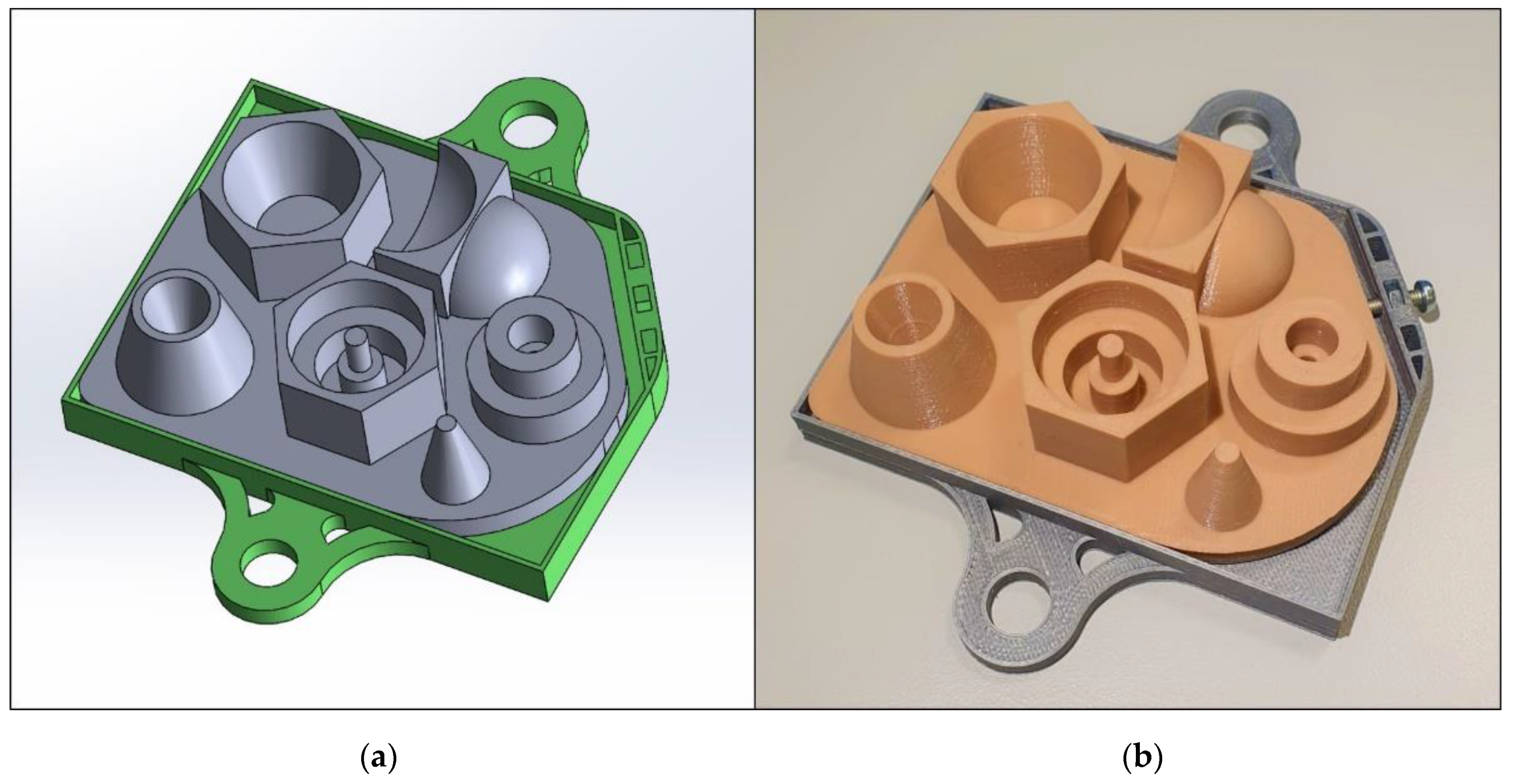
Figure 10.
Artifact designed for the corners of the build space to even out the slice distribution. (a) Spherical surfaces towards the interior of the build space; (b) flat surfaces towards the exterior.
Figure 10.
Artifact designed for the corners of the build space to even out the slice distribution. (a) Spherical surfaces towards the interior of the build space; (b) flat surfaces towards the exterior.

Figure 11.
Slice distribution for all three builds.

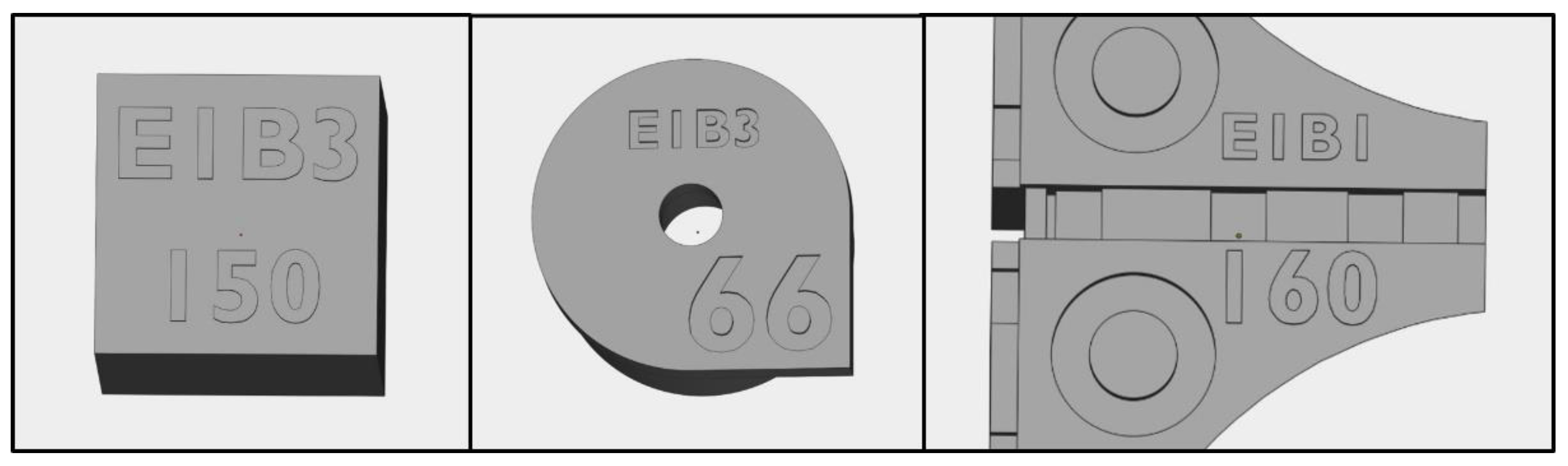
Figure 12.
Labeling of additional models where “E1B3” signifies “experiment 1, build 3” and the final number corresponds to the specimen’s number in the current build.
Figure 12.
Labeling of additional models where “E1B3” signifies “experiment 1, build 3” and the final number corresponds to the specimen’s number in the current build.

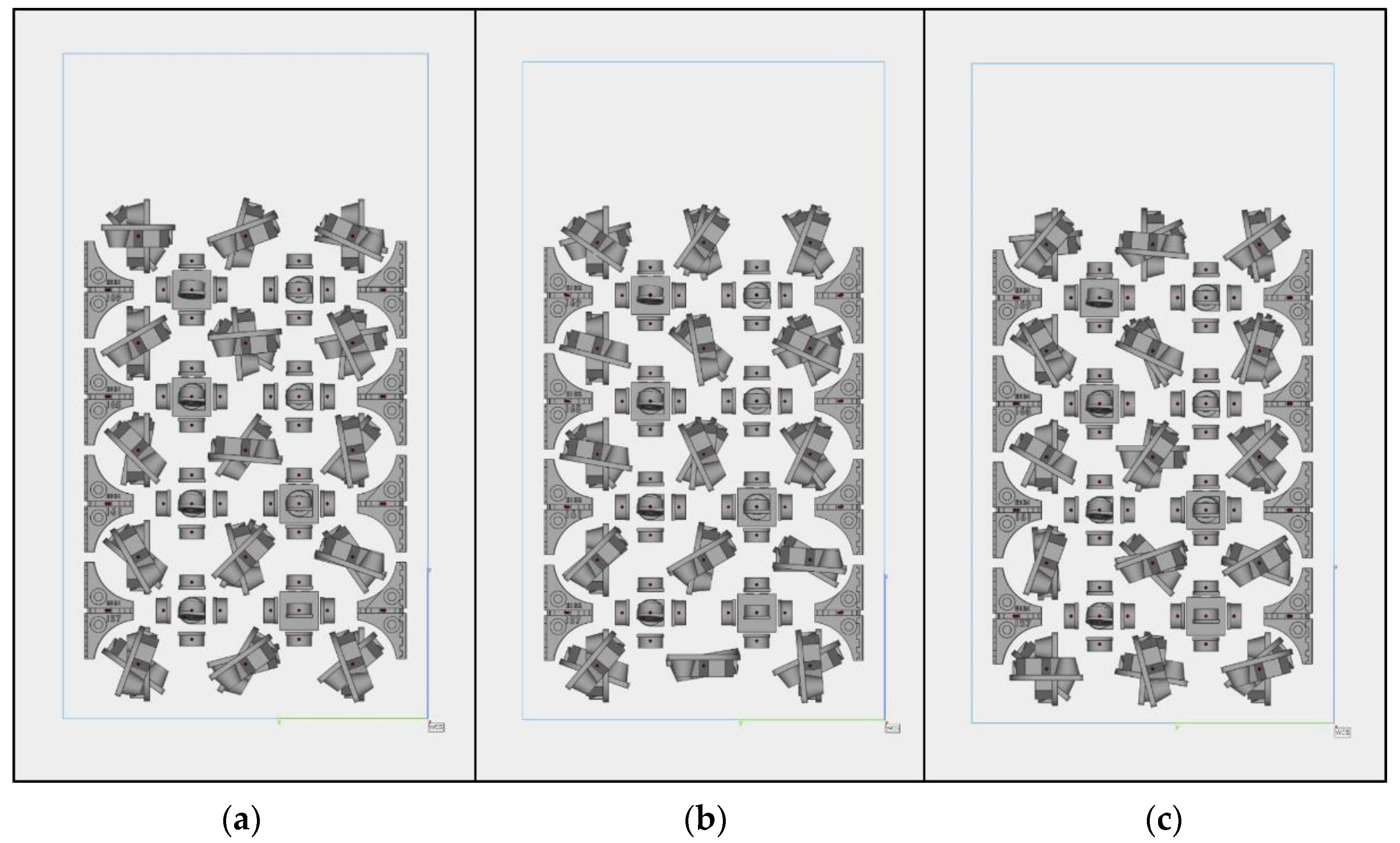
Figure 13.
Build layout in Magics 23.01 for all three builds as seen from the left. (a) Build 1; (b) build 2; (c) build 3.
Figure 13.
Build layout in Magics 23.01 for all three builds as seen from the left. (a) Build 1; (b) build 2; (c) build 3.

Figure 14.
Fixture design for test artifact. (a) Assembled CAD-drawing. (b) The fixture with a prototype of the test artifact in place.
Figure 14.
Fixture design for test artifact. (a) Assembled CAD-drawing. (b) The fixture with a prototype of the test artifact in place.

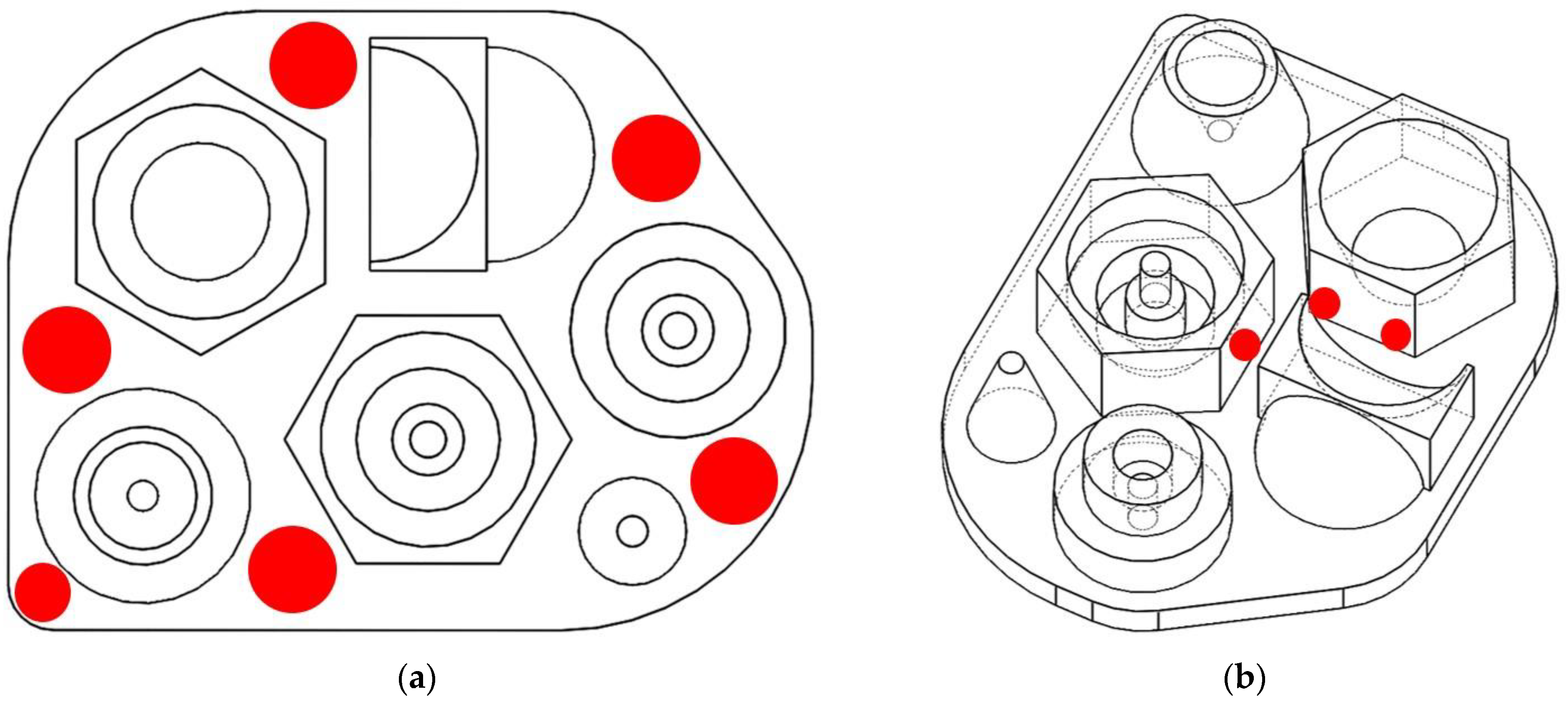
Figure 15.
Manual probing points for base alignment are indicated with red areas. (a) Top view of points on the base plate; (b) a perspective view showing points on HX1 and HX2.
Figure 15.
Manual probing points for base alignment are indicated with red areas. (a) Top view of points on the base plate; (b) a perspective view showing points on HX1 and HX2.

Figure 16.
Inspection strategy for the base plate. A single path follows the edge of the base plate before trailing off towards the interior.
Figure 16.
Inspection strategy for the base plate. A single path follows the edge of the base plate before trailing off towards the interior.

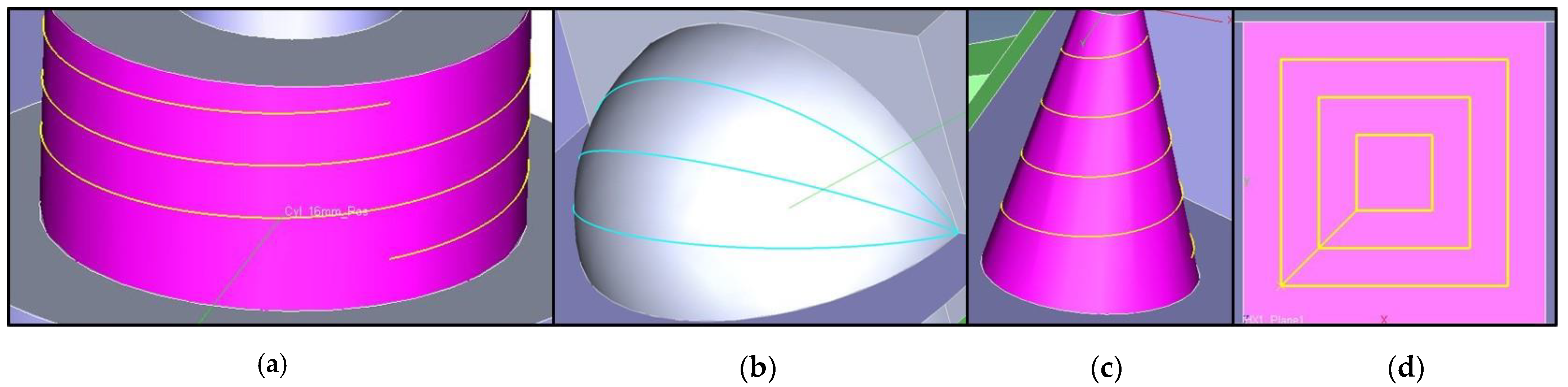
Figure 17.
Illustrations of inspection paths for the different geometries. (a) Helical inspection path for cylinders; (b) three lateral paths for spheres; (c) a helical path for cones; (d) a single continuous path for planes.
Figure 17.
Illustrations of inspection paths for the different geometries. (a) Helical inspection path for cylinders; (b) three lateral paths for spheres; (c) a helical path for cones; (d) a single continuous path for planes.

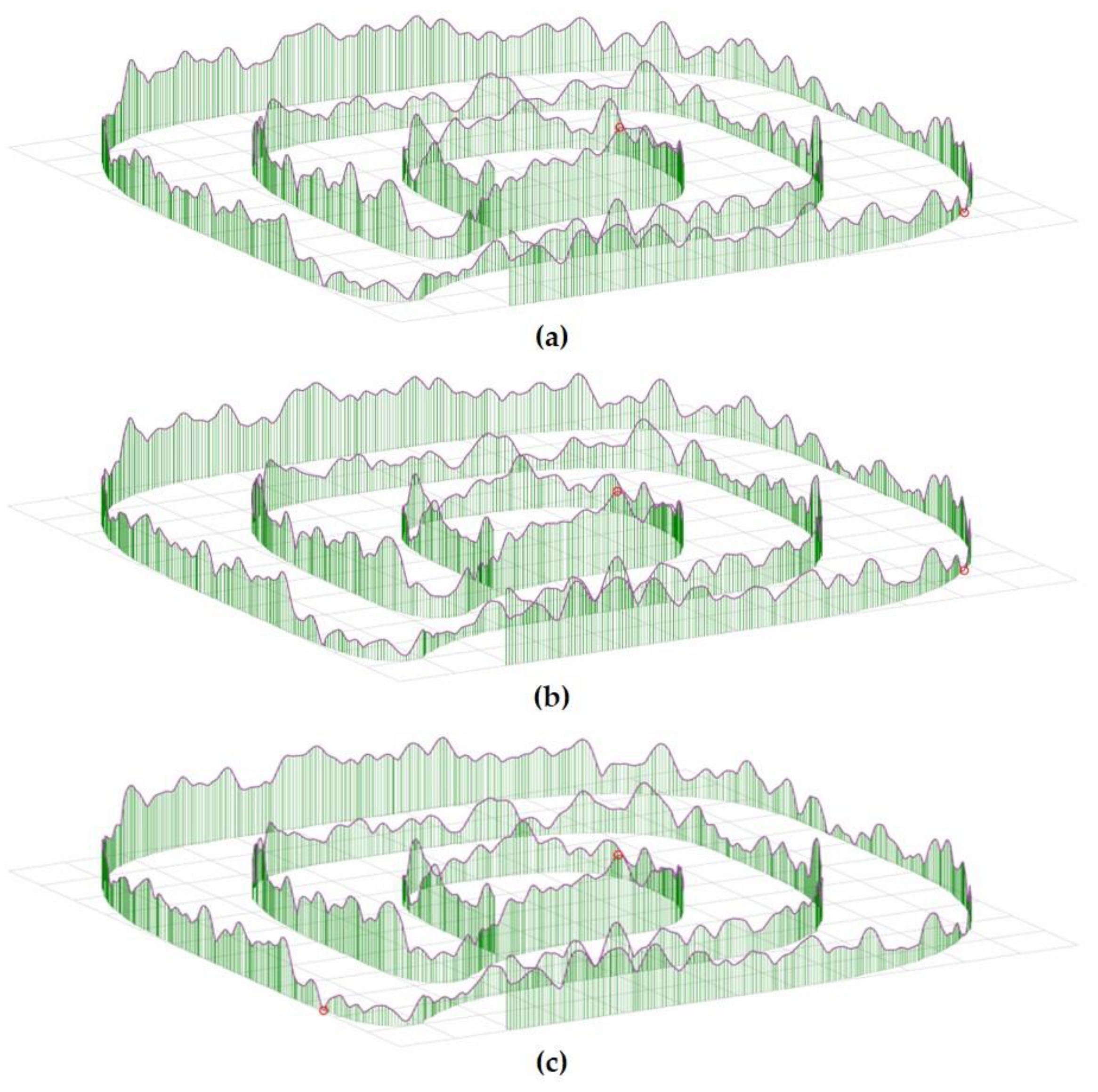
Figure 18.
Plotted results for three repeated inspections for the flatness of Build3_#6_HX1_Plane1 of scale 500:1. Maximum and minimum points for each plot are highlighted with red circles. (a) 1st inspection: 0.062 mm; (b) 2nd inspection: 0.058 mm; (c) 3rd inspection: 0.059 mm.
Figure 18.
Plotted results for three repeated inspections for the flatness of Build3_#6_HX1_Plane1 of scale 500:1. Maximum and minimum points for each plot are highlighted with red circles. (a) 1st inspection: 0.062 mm; (b) 2nd inspection: 0.058 mm; (c) 3rd inspection: 0.059 mm.

Figure 19.
Difference between repeated measurements (∆) of cylindricity, diameter, and flatness. (a) Scatterplot, including all data points; (b) scatterplot only, including data points within five standard deviations (5σ).
Figure 19.
Difference between repeated measurements (∆) of cylindricity, diameter, and flatness. (a) Scatterplot, including all data points; (b) scatterplot only, including data points within five standard deviations (5σ).

Figure 20.
Lognormal probability distributions fitted to the measured data for selected features.

Figure 21.
Comparison of measured error between builds considering vertical planes. (a) A boxplot visualizing the measured flatness error; (b) kernel density estimation of the measured values.
Figure 21.
Comparison of measured error between builds considering vertical planes. (a) A boxplot visualizing the measured flatness error; (b) kernel density estimation of the measured values.

Figure 22.
Comparison of flatness error at different z-positions in the build chamber. (a) Boxplot of all five z-levels; (b) kernel density estimations for the levels of z-positions.
Figure 22.
Comparison of flatness error at different z-positions in the build chamber. (a) Boxplot of all five z-levels; (b) kernel density estimations for the levels of z-positions.

Figure 23.
Boxplot for diametrical error for the anchor specimens across all three builds.

Figure 24.
Boxplot for measured flatness error of vertical planes at different positions. (a) The rows along the x-axis at different z-levels; (b) the rows along the y-axis at different z-levels.
Figure 24.
Boxplot for measured flatness error of vertical planes at different positions. (a) The rows along the x-axis at different z-levels; (b) the rows along the y-axis at different z-levels.

Table 1.
Experiment variables with their designated type/strategy and number of levels.
| Variable | Strategy/Type | Levels | Values |
|---|---|---|---|
| Part build orientation (φ) | Experimental | 37 | |
| Placement in build (P) | Blocking/randomization | 45 | |
| Build ID (B) | Blocking/randomization | 3 | |
| Feature type (F) | Experimental | 4 | |
| Feature size (S) | Experimental | 1–4 | |
| Laser power | Constant | 1 | * |
| Scan speed | Constant | 1 | * |
| Raster pattern | Constant | 1 | * |
| Layer thickness | Constant | 1 | 120 µm * |
| Build chamber temperature | Constant | 1 | 180 °C |
| Room temperature | Regulated | 1 | 20–21 °C † |
| Humidity | Regulated | 1 | 40–50% † |
| Material | Constant | 1 | PA2200 (PA12) |
| Postprocessing | Constant | 1 | Air blasting |
| STL file resolution | Constant | 1 | Tolerances 0.01 mm and 2° |
* given by EOS parameter profile “Balanced”; † approximate range with natural variation. Supplementary data are available in the online repository at GitHub: https://github.com/TheThorb/Leirmo_Exp1_Publication1, accessed on 29 January 2021.
Table 2.
Details on all shape features of the designed artifact.
| Group | Description | Diameter (mm) | Position * (mm) | Normal Vector | ||||
|---|---|---|---|---|---|---|---|---|
| x | y | z | x | y | z | |||
| HX1 | First plane | N/A | 0.00 | −13.86 | 8 | 0 | −1 | 0 |
| Second plane | N/A | 12.00 | −6.93 | 8 | cos(30°) | −0.5 | 0 | |
| Third plane | N/A | 12.00 | 6.93 | 8 | cos(30°) | 0.5 | 0 | |
| Fourth plane | N/A | 0.00 | 13.86 | 8 | 0 | 1 | 0 | |
| Fifth plane | N/A | −12.00 | 6.93 | 8 | −cos(30°) | 0.5 | 0 | |
| Sixth plane | N/A | −12.00 | −6.93 | 8 | −cos(30°) | −0.5 | 0 | |
| HX2 | First plane | N/A | −18.43 | 13.43 | 8 | 0.5 | −cos(30°) | 0 |
| Second plane | N/A | −11.50 | 25.43 | 8 | 1 | 0 | 0 | |
| Third plane | N/A | −18.43 | 37.43 | 8 | 0.5 | cos(30°) | 0 | |
| Fourth plane | N/A | −32.28 | 37.43 | 8 | −0.5 | cos(30°) | 0 | |
| Fifth plane | N/A | −39.21 | 25.43 | 8 | −1 | 0 | 0 | |
| Sixth plane | N/A | −32.28 | 13.43 | 8 | −0.5 | −cos(30°) | 0 | |
| CC1 | Largest cylinder | 24 | 0 | 0 | 8 | 0 | 0 | 1 |
| Second largest cylinder | 16 | 0 | 0 | 0 | 0 | 0 | 1 | |
| Third largest cylinder | 8 | 0 | 0 | 0 | 0 | 0 | 1 | |
| Smallest cylinder | 4 | 0 | 0 | 8 | 0 | 0 | 1 | |
| CC2 | Largest cylinder | 24 | −24.49 | 18 | 0 | 0 | 0 | 1 |
| Second largest cylinder | 16 | −24.49 | 18 | 8 | 0 | 0 | 1 | |
| Third largest cylinder | 8 | −24.49 | 18 | 8 | 0 | 0 | 1 | |
| Smallest cylinder | 4 | −24.49 | 18 | 0 | 0 | 0 | 1 | |
| TC1 | Convex cone | 24 | 21.36 | −24.38 | 0 | 0 | 0 | 1 |
| Concave cone | 12 | 21.36 | −24.38 | 16 | 0 | 0 | −1 | |
| TC2 | Concave cone | 24 | −9.34 | −34.67 | 16 | 0 | 0 | −1 |
| TC3 | Convex cone | 12 | −2.53 | 24.86 | 0 | 0 | 0 | 1 |
| SP | Convex sphere | 24 | −30.84 | −10.3 | 0 | 0 | 0 | 0 |
| Concave sphere | 24 | −24.34 | −21.56 | 13 | 0 | 0 | 0 | |
* the positions of all elements are based on a local origin defined as the center of CC1 for the xy-plane and the top of the base plate in the z-direction. The position of a plane is defined by its center point.
Table 3.
Location and re-orientation of specimen CA_F at edge positions. Rotations A and B signify the counterclockwise rotation about the x- and y-axis, respectively.
Table 3.
Location and re-orientation of specimen CA_F at edge positions. Rotations A and B signify the counterclockwise rotation about the x- and y-axis, respectively.
| Center x | Center y | Rotation A | Rotation B |
|---|---|---|---|
| 120 | 40 | −12.2251 | 4.763642 |
| 220 | 40 | 0 | 0 |
| 300 | 120 | −4.76364 | −12.2251 |
| 300 | 220 | 0 | 0 |
| 220 | 300 | 12.22512 | −4.76364 |
| 120 | 300 | 0 | 0 |
| 40 | 220 | 4.763642 | 12.22512 |
| 40 | 120 | 0 | 0 |
Table 4.
Build process specifications.
| Parameter | Value |
|---|---|
| Machine manufacturer | EOS GmbH—Electro Optical Systems |
| Machine model | EOSINT P395 |
| Parameter profile | Balanced |
| Layer height | 120 µm |
| Hatch distance | 0.3 mm |
| Build chamber temperature | 180 °C |
| Material | PA2200 (PA12) |
| Bulk density | >0.430 * |
| Mean grain size | d50 = 58 * d10 = 40 * d90 = 90 * |
| Material blend | 50% recycled |
* from the material datasheet.
Table 5.
Characteristics with accompanying naming scheme.
| Groups | Characteristic | Characteristic Name |
|---|---|---|
| HX1 HX2 | Flatness | Flatness_<Group>_Plane<#> 1,2 |
| Parallelism | Parallelism_<Group>_<#a>-<#b> 1,2,3 | |
| Distance | Dist_<Group>_<#a>-<#b> 1,2,3 | |
| CC1 CC2 | Cylindricity | Cylindricity_Cyl_<dimension>_<curvature> 4,5 |
| Diameter | Diameter_Cyl_<dimension>_<curvature> 4,5 | |
| Coaxiality | Coaxiality_<Group>_<dim-a>-<dim-a> 1,3,5 | |
| Position | Position_Cyl_<dimension>_<curvature> 4,5 | |
| TC1 TC2 TC3 | Position | Position_Cone_<dimension>_<curvature> 4,5 |
| Apex angle | Cone_Angle_<dimension>_<curvature> 4,5 | |
| Diameter | Diameter_Cone_<dimension>_<curvature>_<altitude> 4,5,6 | |
| SP | Roundness | Roundness_SP_<curvature>_<altitude> 5,6 |
| Position | Position_SP_<curvature> 5 | |
| Profile | Profile_SP_<curvature> 5 | |
| Diameter | Diameter_SP_<curvature>_<altitude> 5,6 |
1 <Group> is the group ID, e.g., “HX1”; 2 <#> is the plane number, e.g., “Plane1”; 3 <a> and <b> refer to the first and last feature in a comparison, respectively; 4 <dimension> and <dim> both refer to the dimension of the feature, e.g., “4 mm” (NB! no space); 5 <curvature> is either “Pos” for convex or “Neg” for concave; 6 <altitude> is “Low”, “Mid” or “Hi”/”Top” where measurements are available at different levels.
Table 6.
A statistical overview of elapsed inspection time for successful inspections.
| Statistic | Elapsed Time (mm:ss) |
|---|---|
| Minimum | 09:20 |
| Median | 10:25 |
| Average | 11:42 |
| Standard deviation | 02:41 |
| Maximum | 18:15 |
Table 7.
Column descriptions for comma-separated values (CSV) files.
| Column Name | Format | Description |
|---|---|---|
| Uuid | 64 hexadecimals + separators | A unique ID for each measurement |
| Characteristic | String | The name of the characteristic |
| K1 measured value | Floating-point number | The measured value |
| K4 time/date | mm/dd/yyyy hh:mm:ss AM/PM | Time and date the inspection was completed |
| K14 part ident | Integer | Repetition number * |
| K53 order number | String | The name of the specimen |
| K2001 characteristic number | Integer | Integer ID for characteristic |
| K2101 nominal value | Floating-point number | The nominal value |
| K2540 direction X | Floating-point number | x-component of the normal vector |
| K2541 direction Y | Floating-point number | y-component of the normal vector |
| K2542 direction Z | Floating-point number | z-component of the normal vector |
| K2543 position X | Floating-point number | x-component of the position |
| K2544 position Y | Floating-point number | y-component of the position |
| K2545 position Z | Floating-point number | z-component of the position |
* measurements are repeated three times. The column “K53 order number” designates, which repetition the measurement represents.
Table 8.
Aggregated data for repeated measurements.
| Rep 1 | Rep 2 | Rep 3 | Rep Mean | ∆ | |
|---|---|---|---|---|---|
| n | 3510 | 3510 | 3510 | – | – |
| 0.088577 | 0.084998 | 0.083011 | 0.085529 | 0.008634 | |
| σ | 0.122123 | 0.118936 | 0.117179 | 0.119282 | 0.011865 |
| Min | −0.544659 | −0.540020 | −0.537463 | −0.540714 | 0.000022 |
| 25% | 0.068541 | 0.066567 | 0.065653 | 0.066977 | 0.002682 |
| 50% | 0.090128 | 0.087218 | 0.086086 | 0.087838 | 0.005521 |
| 75% | 0.132110 | 0.127516 | 0.124374 | 0.127606 | 0.009823 |
| Max | 0.626687 | 0.576267 | 0.542467 | 0.559931 | 0.256032 |
Table 9.
Statistical description of measured flatness error of planes 2 and 5 from HX2 and the difference between the three builds.
Table 9.
Statistical description of measured flatness error of planes 2 and 5 from HX2 and the difference between the three builds.
| Build 1 | Build 2 | Build 3 | Mean | Difference | |
|---|---|---|---|---|---|
| n | 90 | 90 | 90 | – | – |
| 0.100579 | 0.091916 | 0.091149 | 0.094548 | 0.040117 | |
| σ | 0.049281 | 0.028711 | 0.025326 | 0.026291 | 0.040889 |
| Min | 0.058330 | 0.052950 | 0.054538 | 0.065753 | 0.002214 |
| 25% | 0.074281 | 0.072488 | 0.070237 | 0.075634 | 0.019272 |
| 50% | 0.084530 | 0.083260 | 0.085130 | 0.086795 | 0.027337 |
| 75% | 0.105167 | 0.103796 | 0.107094 | 0.103580 | 0.049757 |
| Max | 0.400476 | 0.193571 | 0.162345 | 0.211045 | 0.301388 |
Table 10.
Statistical description of measured flatness error of planes 2 and 5 from HX2 and the difference between the five z-levels.
Table 10.
Statistical description of measured flatness error of planes 2 and 5 from HX2 and the difference between the five z-levels.
| Level 1 | Level 2 | Level 3 | Level 4 | Level 5 | Mean | Difference | |
|---|---|---|---|---|---|---|---|
| n | 54 | 54 | 54 | 54 | 54 | – | – |
| 0.104644 | 0.093710 | 0.096776 | 0.089911 | 0.087698 | 0.094548 | 0.054769 | |
| σ | 0.055572 | 0.031782 | 0.033028 | 0.025317 | 0.024961 | 0.024226 | 0.050230 |
| Min | 0.052950 | 0.059441 | 0.058330 | 0.060803 | 0.054538 | 0.063893 | 0.011309 |
| 25% | 0.071951 | 0.073234 | 0.076536 | 0.072325 | 0.068809 | 0.078640 | 0.025433 |
| 50% | 0.088348 | 0.088711 | 0.084912 | 0.084803 | 0.078242 | 0.087961 | 0.041132 |
| 75% | 0.116436 | 0.104522 | 0.104658 | 0.101218 | 0.102372 | 0.110861 | 0.063584 |
| Max | 0.400476 | 0.222995 | 0.199056 | 0.193571 | 0.167091 | 0.176043 | 0.328619 |
Publisher’s Note: MDPI stays neutral with regard to jurisdictional claims in published maps and institutional affiliations. |
© 2021 by the authors. Licensee MDPI, Basel, Switzerland. This article is an open access article distributed under the terms and conditions of the Creative Commons Attribution (CC BY) license (http://creativecommons.org/licenses/by/4.0/).
Share and Cite
MDPI and ACS Style
Leirmo, T.L.; Semeniuta, O. Investigating the Dimensional and Geometric Accuracy of Laser-Based Powder Bed Fusion of PA2200 (PA12): Experiment Design and Execution. Appl. Sci. 2021, 11, 2031. https://doi.org/10.3390/app11052031
AMA Style
Leirmo TL, Semeniuta O. Investigating the Dimensional and Geometric Accuracy of Laser-Based Powder Bed Fusion of PA2200 (PA12): Experiment Design and Execution. Applied Sciences. 2021; 11(5):2031. https://doi.org/10.3390/app11052031
Chicago/Turabian StyleLeirmo, Torbjørn Langedahl, and Oleksandr Semeniuta. 2021. "Investigating the Dimensional and Geometric Accuracy of Laser-Based Powder Bed Fusion of PA2200 (PA12): Experiment Design and Execution" Applied Sciences 11, no. 5: 2031. https://doi.org/10.3390/app11052031
Note that from the first issue of 2016, this journal uses article numbers instead of page numbers. See further details here.