Nonlinear Control of Multibody Flexible Mechanisms: A Model-Free Approach

Abstract

In this paper a novel nonlinear controller for position and vibration control of flexible-link mechanisms is introduced. The proposed control strategy is model-free and does not require the measurement of the elastic deformation of the mechanism, since the control relies only on the knowledge of the angular position of the actuator and on its time derivative, which can be measured simply with a quadrature encoder. The conditions for the closed-loop stability are evaluated using Lyapunov theory. The performance of the proposed technique is evaluated on a four-bar flexible-link mechanism. Superior vibration damping and more accurate trajectory tracking is obtained in comparison with a PD controller and a fractional order controller, which relies on the same set of measurement as the proposed nonlinear controller.

1. Introduction

Flexible-link robots present several advantages over their rigid counterparts, mainly due to their lightweight construction, which leads to high throughput and low power consumption. On the other hand, they require a clever choice of control strategies [1] and trajectory planning algorithms [2,3] to avoid several vibration-induces issues.

The operation of this kind of mechanisms can be very challenging, due to their inherent lumped actuator dynamics coupled with distributed link dynamics [4]. Exact dynamic models are also required to take into account an infinite-dimensional system. Despite this kind of difficulties, a large number of works on the topic have been published since the 70’s, as testified in the review papers [5,6,7,8]. The majority of the works on the control of flexible-link mechanisms have been conducted on single-link mechanisms or on flexible mechanisms with just one flexible link [9,10,11,12]. In [13,14], the authors deal with flexible multibody mechanisms: in the former, a regulator for controlling a three degree-of-freedom (DOF) planar manipulator with two flexible links is presented, while the latter concerns a three-link planar flexible robot with payload. Therefore, the control of multi-link flexible mechanisms is still an area that requires further investigations.

The reason can be imputed to the fact that the dynamic modeling of flexible multibody mechanisms is a very complex and challenging task. Moreover, if linearized models around a specified operating point are taken into consideration, as done in [15], the dynamics of multi-link flexible mechanisms is described with limited accuracy [16]. As proved experimentally by Milford and Asokanthan in [17], the eigenfrequencies of a two-link flexible robot can vary up to 30% as a function of the manipulator configuration. Several sources, such as [18,19], report that linear models are accurate only for single-link mechanisms. In this sense, model-based control strategies can be very effective, as testified in several papers. In particular, predictive control have proven to be very effective in terms of performance [20,21,22], and have shown sufficient robustness to be a proper choice for flexible multibody mechanisms. It should also be considered that control practitioners often rely on simple models as the basis for model-based controls [1], such as modal systems with a limited number of state variable. In this case, the reduced accuracy in the modeling should be compensated by increasing the robustness properties [23,24] of the controller. This is necessary to avoid the crucial problem of spillover effect, i.e., the neglecting of higher-order modes, which can be a source of instability if combined with linear time-varying parameter perturbations [25,26]. While the research community has proven to be able to cope with these difficulties by including robustness in the control formulation [24,27,28], the solution to the problem is still not within the availability of most industrial applications.

The aim of this paper is to introduce a simple nonlinear control strategy that is shown to be very effective for the simultaneous position control and vibration damping of flexible multibody mechanisms. The proposed approach is of straightforward implementation, has limited computational requirements and, therefore, could be potentially made available to standard industrial control systems. Moreover, the control strategy introduced in this paper has two important characteristics:

• the control is model-free;
• the control relies on one measured variable only.

The first characteristic is fundamental in all industrial applications, where the required knowledge to operate with complex nonlinear models is not often found. The field of application of the proposed solution is further enlarged, since the control strategy relies only on the measurement of the angular position of the mechanism, which can be easily obtained with quadrature encoders.

The paper is outlined as follows: Section 2 briefly recalls the dynamic modeling of planar flexible mechanisms used for the numerical evaluation and the proof of stability of the proposed control strategy. Control design and stability conditions are explained in Section 3, whereas Section 4 reports some numerical evaluation of the closed-loop performance and a comparison with PD control and fractional order PD${}^{\mu }$ controllers. The conclusions are given in Section 5.

2. Dynamic Model of Multibody Flexible-Link Mechanisms

In this section, the analytic model of a generic planar multibody mechanism composed of flexible links is briefly explained. The complete development of the equations of motion can be found in [29] together with an experimental validation of the accuracy of the model. The same dynamic model has been validated and used in several works, such as in [30] for the development of predictive control strategies for position control and vibration damping, and in [31] for the development of state observers for flexible-link mechanisms. Recently, such model has also been extended to 3D mechanisms in [32,33,34]. The dynamic model of flexible-link planar mechanisms is based on an Equivalent Rigid-Link System (ERLS) formulation, and on the use of a discretization based on the finite element method (FEM). First of all, each link of the mechanism must be divided into finite elements. The kinematics of the mechanism, which can have either a closed-loop kinematic chain or an open-loop one, is defined by means of the following vectors, measured in the fixed global reference frame $\{X,Y,Z\}$: ${\mathbf{r}}_i$ and ${\mathbf{u}}_i$ are the vectors of nodal position and nodal displacement in the i-th element of the ERLS and of their elastic displacement, respectively; ${\mathbf{p}}_i$ is the position of a generic point inside the i-th element; $\mathbf{q}$ is the vector of the generalized coordinates of the ERLS. The relationship between these vectors is shown in Figure 1.

The application of the principle of virtual works, which states that the sum of the virtual works of inertial, elastic and external forces is equal to zero, leads to:

$$\sum _i{\int }_{{\mathbf{v}}_i}\delta {\mathbf{p}}_i^T{\ddot{\mathbf{p}}}_i\mathrm{d}\nu +\sum _i{\int }_{{\mathbf{v}}_i}\delta {ϵ}_i^T{\mathbf{D}}_i{ϵ}_i\mathrm{d}\nu =\sum _i{\int }_{{\mathbf{v}}_i}\delta {\mathbf{p}}_i^T\mathbf{g}\rho \mathrm{d}\nu +(\delta {\mathbf{u}}^T+\delta {\mathbf{r}}^T)\mathbf{F}$$

(1)

${ϵ}_i$, ${\mathbf{D}}_i$, ${\rho }_i$ and $\delta {ϵ}_i$ are the strain vector, the stress-strain matrix, the mass density of the i-th link and the virtual strains, respectively. $\mathbf{F}$ is the vector of the external forces, including gravity. Equation (1) shows the virtual works of inertial, elastic an external forces, respectively. From this equation, ${\mathbf{p}}_i$ and ${\ddot{\mathbf{p}}}_i$ can be evaluated, for a generic point of the i-th link from:

$$\delta {\mathbf{p}}_i={\mathbf{R}}_i{\mathbf{N}}_i{\mathbf{T}}_i\delta {\mathbf{r}}_i$$

(2)

$${\ddot{\mathbf{p}}}_i={\mathbf{R}}_i{\mathbf{N}}_i{\mathbf{T}}_i+2({\dot{\mathbf{R}}}_i{\mathbf{N}}_i{\mathbf{T}}_i+{\mathbf{R}}_i{\mathbf{N}}_i{\dot{\mathbf{T}}}_i){\dot{\mathbf{u}}}_i$$

(3)

where ${\mathbf{T}}_i$ is a matrix that describes the transformation from global to local reference frame of the i-th element, ${\mathbf{R}}_i$ is the local-to-global rotation matrix, and ${\mathbf{N}}_i$ is the shape function matrix, which is obtained using a proper FEM description. Taking ${\mathbf{B}}_i(x_i,y_i,z_i)$ as the strain-displacement matrix, the following relations holds:

$${ϵ}_i={\mathbf{B}}_i{\mathbf{T}}_i\delta {\mathbf{u}}_i$$

(4)

$$\delta {ϵ}_i={\mathbf{B}}_i\delta {\mathbf{N}}_i{\mathbf{T}}_i{\mathbf{u}}_i+{\mathbf{B}}_i{\mathbf{N}}_i{\mathbf{T}}_i\delta {\mathbf{u}}_i$$

(5)

Since nodal elastic virtual displacements $\delta \mathbf{u}$ and nodal virtual displacements of the ERLS $\delta \mathbf{r}$ are independent from each other, the equations of motion of the system can be written as:

$$\begin{array}{c}\mathbf{M}\ddot{\mathbf{u}}+\mathbf{MS}\ddot{\mathbf{q}}=\mathbf{f}\left(\mathbf{u},\dot{\mathbf{u}},\mathbf{q},\dot{\mathbf{u}}\right)\\ {\mathbf{S}}^T\mathbf{M}\ddot{\mathbf{u}}+{\mathbf{S}}^T\mathbf{MS}\ddot{\mathbf{q}}={\mathbf{S}}^T\mathbf{f}\left(\mathbf{u},\dot{\mathbf{u}},\mathbf{q},\dot{\mathbf{u}}\right)\end{array}$$

(6)

$\mathbf{M}$ is the mass matrix of the whole system and S is the sensitivity matrix for all the nodes. Vector $\mathbf{f}=\mathbf{f}(\mathbf{u},\dot{\mathbf{u}},\mathbf{q},\dot{\mathbf{q}})$ includes all the forces acting on the system, with the exception of the inertial forces. By adding the Rayleigh damping, the right-hand side of Equation (6) becomes:

$$\begin{array}{c}\left[\begin{array}{c}\mathbf{f}\\ {\mathbf{S}}^T\mathbf{f}\end{array}\right]:=\left[\begin{array}{ccc}-2{\mathbf{M}}_G-\alpha \mathbf{M}-\beta \mathbf{K}& -\mathbf{M}\dot{\mathbf{S}}& -\mathbf{K}\\ {\mathbf{S}}^T(-2{\mathbf{M}}_G-\alpha \mathbf{M})& -{\mathbf{S}}^T\mathbf{MS}& \mathbf{0}\end{array}\right]\left[\begin{array}{c}\dot{\mathbf{u}}\\ \dot{\mathbf{q}}\\ \mathbf{u}\end{array}\right]+\left[\begin{array}{cc}\mathbf{M}& \mathbf{I}\\ {\mathbf{S}}^T\mathbf{M}& {\mathbf{S}}^T\mathbf{MS}\end{array}\right]\left[\begin{array}{c}\mathbf{g}\\ \mathbf{F}\end{array}\right]\hfill \end{array}$$

(7)

Matrix ${\mathbf{M}}_G$ accounts for the Coriolis contribution, while $\mathbf{K}$ is the stiffness matrix of the whole mechanism. $\alpha$ and $\beta$ are the Rayleigh damping coefficients. The system of differential equations in (6) and (7) can be made solvable by forcing to zero as many elastic displacement as the generalized coordinates. In this way, the ERLS position is defined unequivocally. By removing the displacements forced to zero from Equations (6) and (7), an operation indicated by the operator ${ }^{†}$, the following equation is obtained:

$$\left[\begin{array}{cc}{\mathbf{M}}^{†}& {\left(\mathbf{MS}\right)}^{†}\\ {\left({\mathbf{S}}^T\mathbf{MS}\right)}^{†}& {\mathbf{S}}^T\mathbf{MS}\end{array}\right]\left[\begin{array}{c}{\ddot{\mathbf{u}}}^{†}\\ \ddot{\mathbf{q}}\end{array}\right]=\left[\begin{array}{c}{\mathbf{f}}^{†}\\ {\mathbf{S}}^T\mathbf{f}\end{array}\right]$$

(8)

In this way, the values of the accelerations can be computed at each step by solving the system in Equation (8), while the values of velocities and displacements can be obtained by an appropriate integration scheme, provided that the integration step is set to a sufficiently small value.

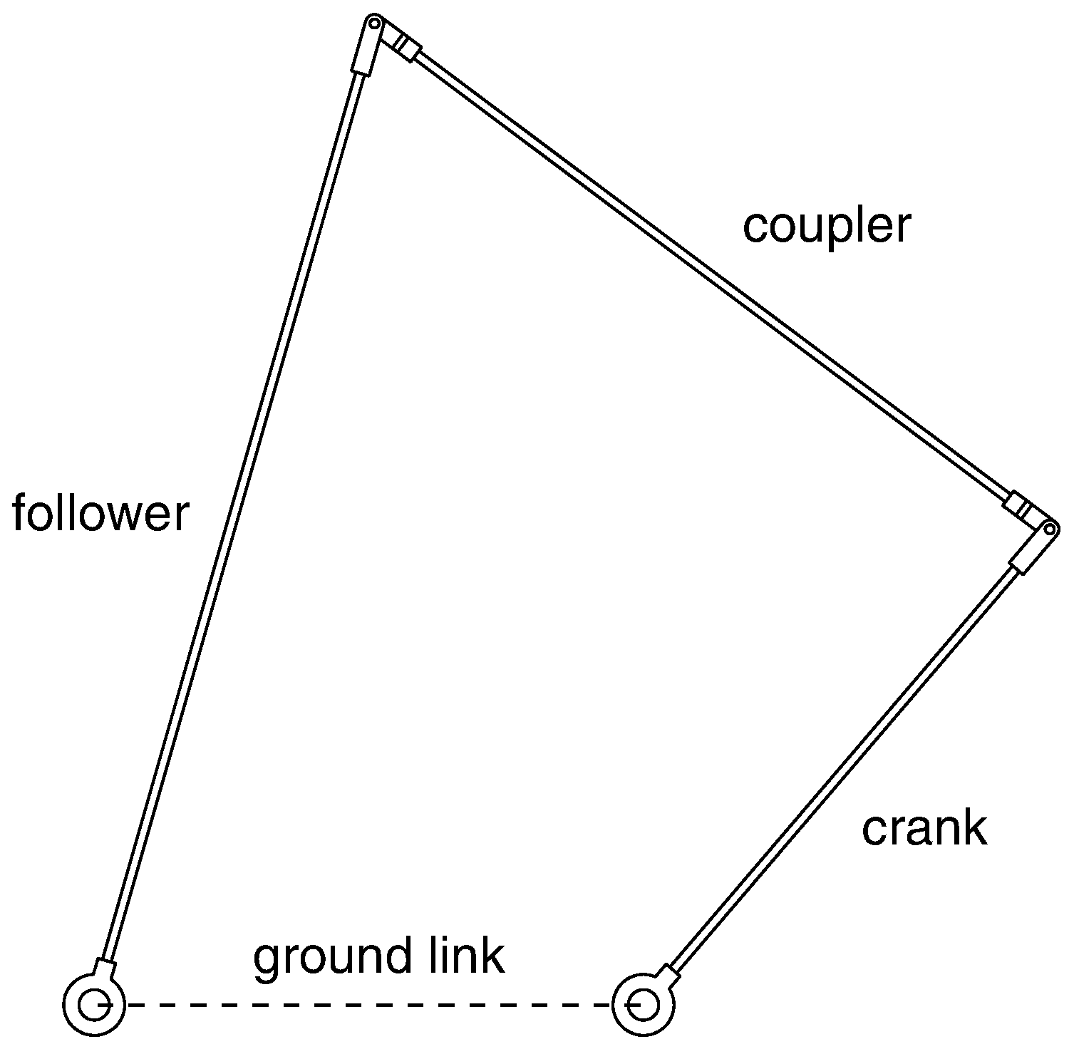
The structure of the mechanism taken into account for the numerical simulations is depicted in Figure 2. The mechanical parameters and the corresponding values are reported in

Table 1. Mechanical parameters of the flexible mechanism.

Parameter	Value
crank length	0.373 m
coupler length	0.525 m
follower length	0.632 m
ground link length	0.36 m
beam width	6 mm
beam thickness	6 mm
Young’s modulus	2 × 10${}^{11}$ N/m${}^2$
flexural inertia moment	11.102 × 10${}^{-2}$ m${}^4$
link mass/length	0.272 kg/m
Rayleigh damping $\alpha$	8.7 × 10${}^{-2}$
Rayleigh damping $\beta$	2.1 × 10${}^{-5}$

. The finite element discretization of the mechanisms uses one finite element for the crank and the coupler links, while the follower, i.e., the longest link, is discretized with two finite elements. The ground link is considered to be perfectly rigid. The total number of elastic displacement for all the links taken as separated would be 21, but after assembling the mechanism and consequently taking into account the coupling between the links, the number of nonzero elastic displacement is reduced to 12. A visual representation of the elastic displacements is provided in Figure 3.

The simulation results reported in Section 4 are provided, as regards the elastic motion, in terms of the link curvature instead of in terms of nodal elastic displacements, the latter being of less direct interpretation.

3. Nonlinear Control Design

The proposed control algorithm is based on the following control action:

$$\tau \left(t\right)=k_p(q^{*}-q\left(t\right))-k_d\dot{q}\left(t\right)-k_n\dot{q}\left(t\right){\left(q^{*}-q\left(t\right)\right)}^2$$

(9)

being $q^{*}$ the reference for the angular position of the mechanism $q\left(t\right)$. $k_p$, $k_d$ and $k_n$ are scalar quantities that represent the tuning parameters of the controller. The control action is nonlinear, given the presence of the term $k_n\dot{q}\left(t\right){\left(q^{*}-q\left(t\right)\right)}^2$. In the following, it will be shown that the nonlinear control action, without which the control acts as a pure PD controller, can be effectively used to improve the damping of high frequency vibration induced on the mechanism during the motion. The PD controller is often used for the control of this class of mechanisms, since the derivative action acts as a damping factor for the elastic displacement. A notable work on the subject [35] also reports that any flexible-link mechanism, even in the presence of gravity, can be asymptotically stabilized by a simple joint PD controller, therefore without the need to measure elastic displacements.

The proposed controller belongs to the wide class of nonlinear PID control, according to the definition of [36], which lists in this class any PID control with time-varying proportional, derivative and integral gains. The use of nonlinear PID controllers is recognized by the capability of improving the performance when used to control nonlinear plants, or to improve damping, tracking accuracy or to reduce rise time for rapid inputs for linear plant. The control law (9) can be written as a PD control with a nonlinear derivative gain described by the equivalent gain $k_d^{\prime }\left(t\right)=k_d+k_n{\left(q^{*}-q\left(t\right)\right)}^2$, and, therefore, as a derivative gain modulation based on the magnitude of the state of the plant, according to [36]. The numerical results provided in this work will show that the modulation of the derivative gain can improve both the position tracking and the vibration damping for fast-changing reference signals.

The conditions for the stability of the closed loop system can be derived by taking into account the following Lyapunov function:

$$V\left(t\right)=E_k\left(t\right)+E_p\left(t\right)+{\displaystyle \frac{k_p}{2}}{(q^{*}-q\left(t\right))}^2$$

(10)

$E_k\left(t\right)$ and $E_p\left(t\right)$ are the kinetic and the potential energy of the mechanism, that cannot assume negative values. If $k_p$ is a positive scalar, also $V\left(t\right)\ge 0$. According to Barbalat’s lemma [37], the asymptotic stability can be proved if $V\left(t\right)$ is lower bounded, $\dot{V}\left(t\right)$ is negative definite, and $\dot{V}\left(t\right)$ is uniformly continuous in time.

Let us verify also the second condition imposed by Barbalat’s lemma. The time derivative of $V\left(t\right)$ is:

$$\dot{V}\left(t\right)={\dot{E}}_k\left(t\right)+\dot{E_p}\left(t\right)-\dot{q}\left(t\right)k_p(q^{*}-q\left(t\right))$$

(11)

If damping is neglected from the dynamic model of the mechanism, under conservative conditions, the variation of the total energy of the system over a time t is only due to the work done by the actuator over the same time interval:

$$\Delta E_k\left(t\right)+\Delta E_p\left(t\right)={\int }_0^t\tau \left(s\right)\dot{q}\left(s\right)\mathrm{d}s$$

(12)

being $\tau$ the torque provided by the actuator. The time derivative of (12) is:

$${\dot{E}}_k\left(t\right)+{\dot{E}}_p\left(t\right)=\tau \left(t\right)\dot{q}\left(t\right)$$

(13)

which, substituted into (11), leads to:

$$\dot{V}\left(t\right)=\tau \left(t\right)\dot{q}\left(t\right)-\dot{q}\left(t\right)k_p(q^{*}-q\left(t\right))$$

(14)

Using the formulation of the control torque $\tau \left(t\right)$ as defined in (9), the last equation leads to:

$$\begin{array}{c}\dot{V}\left(t\right)=\dot{q}\left(t\right)\left(k_p(q^{*}-q\left(t\right))-k_d\dot{q}\left(t\right)-k_n\dot{q}{(q^{*}-q\left(t\right))}^2\right)-\dot{q}\left(t\right)k_p(q^{*}-q\left(t\right))\end{array}$$

(15)

which can also be written as:

$$\dot{V}\left(t\right)=-{\dot{q}}^2\left(t\right)\left(k_n{(q^{*}-q\left(t\right))}^2+k_d\right)$$

(16)

The derivative of the Lyapunov function $\dot{V}\left(t\right)$ is negative as long as the term $k_n{(q^{*}-q\left(t\right))}^2+k_d$ is positive, i.e., if $k_n{(q^{*}-q\left(t\right))}^2>-k_d$. Under this condition, the closed loop system is dissipative and global stability is guaranteed. It should be mentioned that this condition is quite conservative, since it does not take into account the dissipative action of the damping terms neglected in the Lyapunov candidate function in (12).

The third condition imposed by Barbalat’s lemma is met if $\dot{V}\left(t\right)$ is uniformly continuous. According to [23], a sufficient condition for the uniform continuity of $\dot{V}\left(t\right)$ is the boundedness of $\ddot{V}\left(t\right)$. The latter condition will be demonstrated here.

First of all, $V\left(t\right)\le V\left(0\right)$ for every $t\ge 0$, as a consequence of the results presented so far. On the other hand, $V\left(t\right)$ is the sum of nonnegative terms (see Equation (10)). Therefore, the boundedness of $V\left(t\right)$ implies the boundedness of all the three terms on the right-hand side of Equation (10). The boundedness of the kinetic energy $E_k\left(t\right)$ also implies the boundedness of $\dot{q}\left(t\right)$ and of $\dot{u}\left(t\right)$. At the same time, the existence of bounds on the potential energy $E_p\left(t\right)$ implies that $u\left(t\right)$ is bounded [35]. Therefore, also $\tau \left(t\right)$ is bounded, according to the control law in Equation (9). Now, from Equation (16), the second time derivative of the Lyapunov candidate function is:

$$\ddot{V}\left(t\right)=-2\dot{q}\left(t\right)\ddot{q}\left(t\right)\left(k_n{\left(q^{*}-q\left(t\right)\right)}^2+k_d\right)+2k_n{\dot{q}}^3\left(t\right)q\left(t\right)$$

(17)

This equation clearly shows that if also $\ddot{q}\left(t\right)$ is bounded, then $\ddot{V}\left(t\right)$ is bounded as well. On the other hand, the boundedness of $\tau \left(t\right)$ implies the boundedness of the vector of external forces $\mathbf{f}$ that appears in (7), both in the presence and the absence of gravity force. Now, Equation (8) can be rewritten as:

$$\left[\begin{array}{c}\ddot{\mathbf{u}}\\ \ddot{\mathbf{q}}\end{array}\right]={\left[\begin{array}{cc}{\mathbf{M}}^{†}& {\left(\mathbf{MS}\right)}^{†}\\ {\left({\mathbf{S}}^T\mathbf{MS}\right)}^{†}& {\mathbf{S}}^T\mathbf{MS}\end{array}\right]}^{-1}\left[\begin{array}{c}{\mathbf{f}}^T\\ {\mathbf{S}}^T\mathbf{f}\end{array}\right]$$

(18)

Up to now it has been shown that $\mathbf{t}\left(\mathbf{u},\dot{\mathbf{u}},\mathbf{q},\dot{\mathbf{q}}\right)$ is bounded, and as the consequence of the boundedness of $\dot{\mathbf{q}}$ also the sensitivity matrix $\mathbf{S}$ is bounded. Therefore, the left-hand side of Equation (18) is bounded as long as the matrix inversion can be performed. But the matrix inversion can be performed as long as the mechanism does not encounter, during the motion, any singular configuration, and this condition is met provided that a proper choice of the zeroed elastic displacement is made [29]. Now, if the left-hand side of (18) is bounded, also $\ddot{\mathbf{q}}\left(t\right)$ and consequently $\ddot{V}\left(t\right)$ are bounded as well, according to (17). Therefore, all the conditions imposed by Barbalat’s lemma are met and the control is stable, provided that the control tuning parameters are set within the above prescribed limits.

Application to Speed-Controlled Robots

The proposed control action of Equation (9) is designed to work with torque-controlled robots. A more frequent case, in industrial applications, is the use of speed-controlled robots, i.e., the motor drive is set-up in order to follow a joint speed trajectory that is either precomputed or generated in real-time by a suitable closed-loop controller. Therefore, a possible modification to the control action of Equation (9) is the following control law:

$$u^{*}\left(t\right)=k_1\left(q^{*}-q\left(t\right)\right)+k_2{\left(q^{*}-q\left(t\right)\right)}^3+k_3{\int }_0^t\left(q^{*}-q\left(t\right)\right)\mathrm{d}t$$

(19)

The tuning parameters $k_1$, $k_2$ and $k_3$ are fixed scalar quantities, and $u^{*}\left(t\right)$ it the reference signal to be fed to the speed control. A direct comparison between (9) and (19) reveals that the first controller acts as a proportional-derivative controller augmented with a nonlinear derivative action, while the second controller is essentially a proportional-integrative controller augmented with a nonlinear proportional action. In other words, for the first controller the modulation of gain happens on the derivative action, while for the second one it happens on the proportional action. If the inertia J of a single-joint robot can be approximated by a constant value, the acceleration of the joint is proportional to the torque $\tau$, through the obvious relationship $J\ddot{q}\left(t\right)=\tau \left(t\right)$. If the first control is used, the last one can be rewritten using Equation (9) as:

$$J\ddot{q}\left(t\right)=\tau \left(t\right)=k_p(q^{*}-q\left(t\right))-k_d\dot{q}\left(t\right)-k_n\dot{q}\left(t\right){\left(q^{*}-q\left(t\right)\right)}^2$$

(20)

Now, considering a properly tuned robot actuated by a speed-controlled drive, with the additional feedback control of (19), Equation (20) can be written as:

$$J\ddot{q}\left(t\right)=J\frac{d}{dt}{u}^{*}\left(t\right)=-J{k}_1\dot{q}\left(t\right)-3J{k}_2\dot{q}\left(t\right){\left(q^{*}-q\left(t\right)\right)}^2+J{k}_3\left(q^{*}-q\left(t\right)\right)$$

(21)

A direct comparison between (20) and (21) shows that the equivalence between the two controllers happens when $k_p=J{k}_3$, $k_d=J{k}_1$, $k_n=3J{k}_2$. Such equivalence shows that the proposed strategy can be used for both torque-controlled systems and speed-controlled systems, retaining the same level of performance in both cases. The proof of the stability of the controller of Equation (19) is omitted, since the stability bounds can be assessed using the same procedure already developed to prove the stability of the control (9), using the candidate Lyapunov function $V\left(t\right)=T\left(t\right)+U\left(t\right)+J\frac{k_3}{2}{\left(q^{*}-q\left(t\right)\right)}^2$. The resulting stability bound on control gains is:

$$k_1+3k_2{\left(q^{*}-q\left(t\right)\right)}^2\ge 0$$

(22)

The control laws of (9) and (19) both require either a measurement or an estimation of the angular speed of the joint $\dot{q}\left(t\right)$. A rough estimation of the joint speed can be achieved using numerical differentiation. Such method, while being of straightforward application, can lead to high-frequency spurious signals [38,39] that can reduce the effectiveness or even jeopardize the stability of the closed-loop system, especially when using low-resolution encoders or high derivative gains. For this reason, a good practice is to make use of observers [38] or other filtering techniques [39,40].

4. Control Tuning and Closed-Loop Response

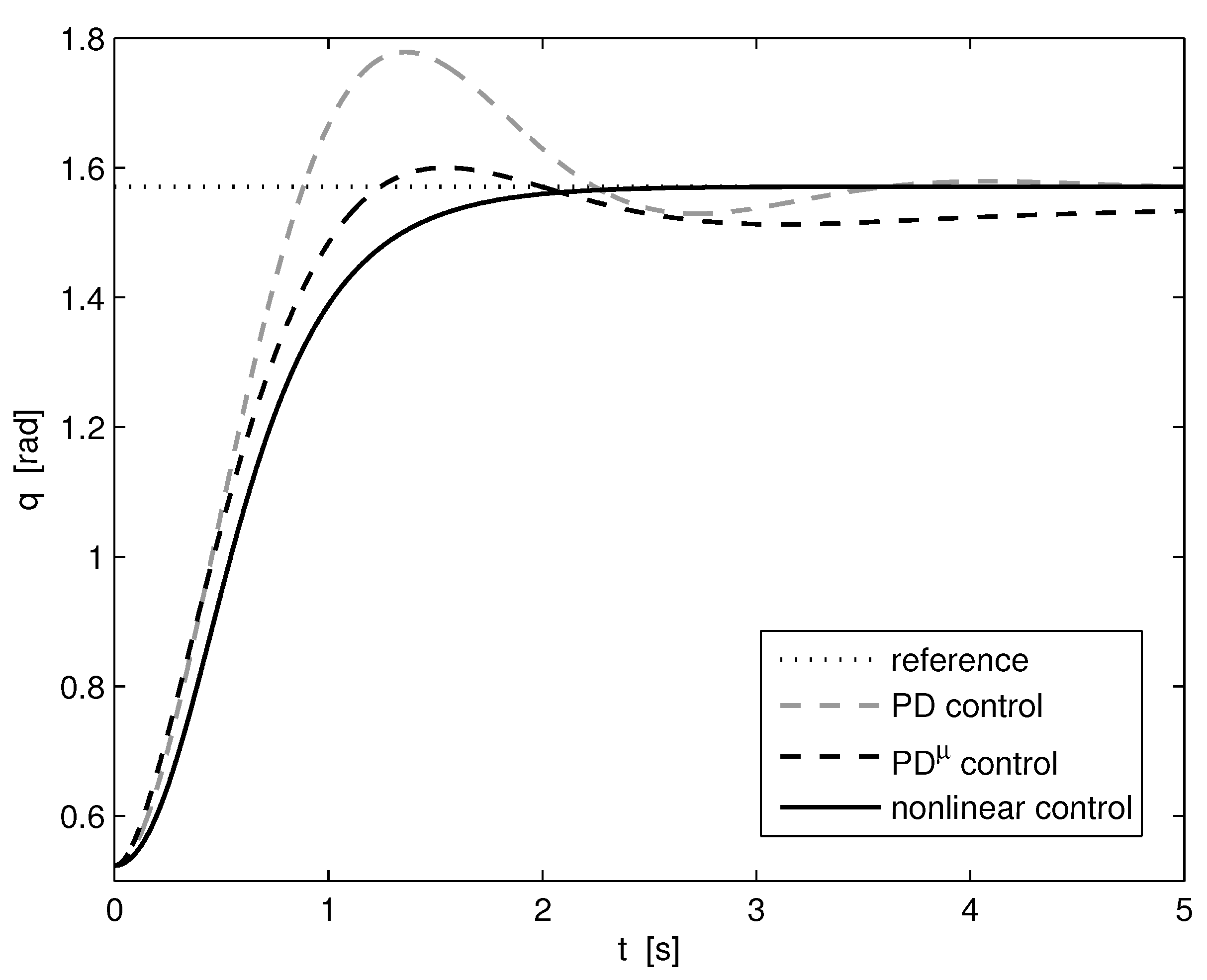
In this section, the effectiveness of the proposed control law is investigated numerically. The plant used as the test bench is the four-bar linkage described in Section 2. All the tests presented here involve the tracking of a step signal for the angular position of the crank q. The target position is $q^{*}=\pi /2$ rad, while the initial position of the mechanism is $q\left(0\right)=\pi /6$ rad. The effectiveness of the control system is evaluated on the basis of the precision and speed of tracking of the reference signal, but also in terms of vibration damping. The latter is accomplished by measuring the curvatures at the midspan of the crank and of the follower links.

The evaluation of the performance is obtained through a comparison with two other control strategies, which share with the proposed controller the use of a single measurement, i.e., the angular position of the crank, and the model-free approach. Moreover, all three controllers are joint controllers, since they rely on measurements made to the actuated joint, and they do not explicitly take into account the elastic behavior of the mechanism.

Fractional order control [41], that in its more general form is referred as PI${}^{\lambda }$D${}^{\mu }$ control, is a control system based on fractional calculus, i.e., a generalization of standard calculus that takes into account integrals and derivatives of non-integer order [42]. In particular, a PI${}^{\lambda }$D${}^{\mu }$ control will have a standard proportional action, an integral action of order $\lambda$, and a derivative action of order $\mu$. For the particular case in which $\lambda =\mu =1$, the fraction order PID control and the standard PID control are perfectly equivalent. The PD${}^{\mu }$ control used for the numerical simulation reported in this work has been developed using FOMCON toolbox [43]. Since the exact computation of a fractional order PID control is not possible, being such controller an infinite dimension linear filter [44], a finite size approximation is needed for a real-time implementation. Several approximation techniques have been proposed in the literature [41], the one used in this work is the Oustaloup’s approximation [45], which is included in the FOMCON toolbox.

Figure 4 shows the behaviour of all three controllers in terms of angular position tracking. From the figure it can be clearly seen that the most accurate tracking, i.e., the one with null overshoot and minimal settling time, is achieved with the nonlinear control. The PD control produces a large overshoot, while PD${}^{\mu }$ leads to smaller overshoot with respect to the PD control, but at the same time requires a longer settling time. The tuning of the three controllers, whose parameters are reported in

Table 2. Control tuning parameters.

Control	Tuning Parameters
PD control	$k_p=$ 0.15; $k_d=$ 0.04
PD${}^{\mu }$ control	$k_p=$ 0.0165; $k_d=$ 0.067; $\mu =$ 0.68
nonlinear control	$k_p=$ 0.08; $k_d=$ 0.09; $k_n=$ −0.08

, has been set to achieve similar rise times.

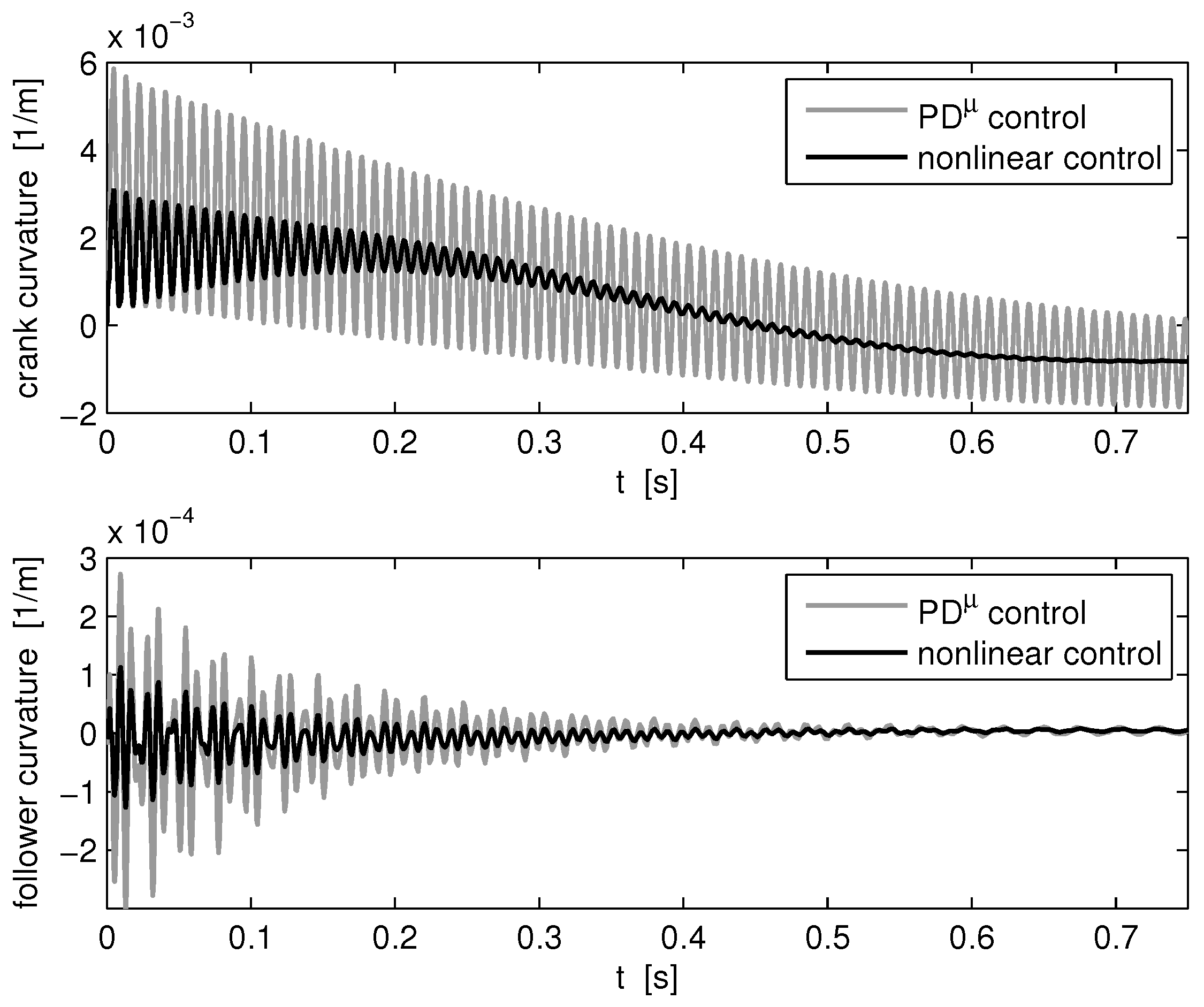
The results of the same three tests are shown in Figure 5 and Figure 6 in term of link curvatures of the crank and follower link, respectively. In both cases, it can be clearly seen that the nonlinear control performs better than both PD and PD${}^{\mu }$ controllers as far as vibration damping is taken into account. The time needed to dampen the elastic motion of both links is remarkably high for the PD controller, whereas the PD${}^{\mu }$ and the nonlinear control have similar damping properties.

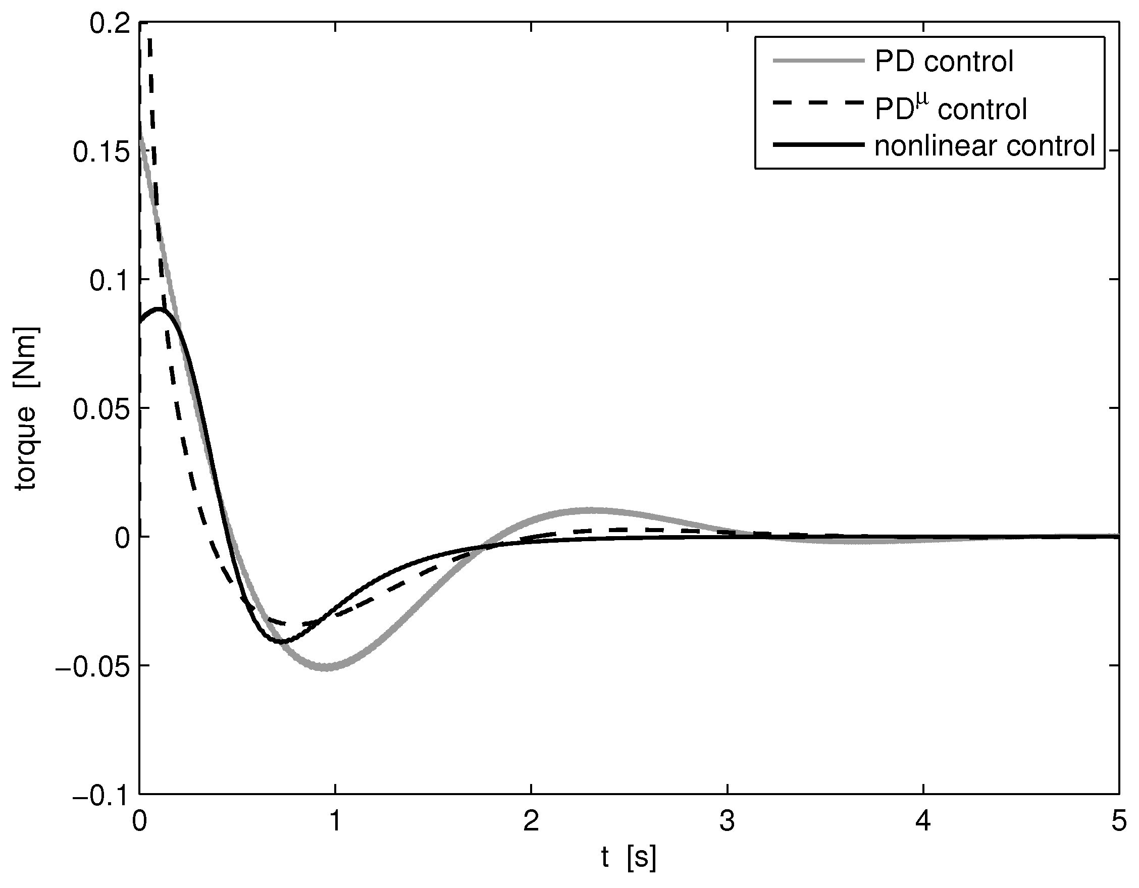
A more accurate comparison of the damping capability of the nonlinear controller can be deduced from the results presented in Figure 7, in which the response is plotted over an interval of 0.75 s. This comparison shows again that the nonlinear control has clearly a more pronounced damping effect, and that also the amplitude of vibration at the very beginning of the motion is less pronounced. This behavior can also be explained by looking at the torque profiles reported in Figure 8. From the figure, it can be clearly seen that the PD${}^{\mu }$ controller produces an intense control action at the beginning of the motion, which induces pronounced vibrations. Furthermore, the PD controller has a very aggressive control effort at the beginning of motion. This is due to the fact that vibration damping in this kind of control requires to set the derivative gain $k_d$ to a quite high value, with the side effect of slowing down also the position tracking. At the same time, the $k_p$ gain of the PD controller needs to be set to an high value to compensate the speed reduction introduced by the derivative term, with the consequence of leading also to a pronounced overshoot (see Figure 4).

The proposed nonlinear control is capable of avoiding this occurrence: the nonlinear action governed by the gain $k_n$, which is set to a negative value, basically reduces the effects of derivative action when the tracking error is high, i.e., during the first part of the transient. This momentary reduction of derivative action does not need to be compensated by an aggressive proportional gain, which would lead to pronounced vibrations at the beginning of the transient. Figure 8 actually shows that the nonlinear control produces a peak torque that is reduced by 47% in comparison with PD control and by 56% in comparison with PD${}^{\mu }$ control. The maximum values of the motor torque developed by the three control systems is reported in

Table 3. Performance measurement and comparison between PD, PD${}^{\mu }$ and nonlinear controller.

Performance Measurement	$\mathbf{PD}$	${\mathbf{PD}}^{\mathit{\mu }}$	Nonlinear Control
Settling time [$\pm 5\%$]	2.022 s	3.685	1.455
Vibration settling time $[\pm 1\times {10}^{-4}$m${}^{-1}]$	0.2775 s	0.1616 s	0.0329 s
Overshoot [%]	19.8%	2.8%	0.006%
Peak torque [Nm]	0.157 Nm	0.2 Nm	0.088 Nm

.

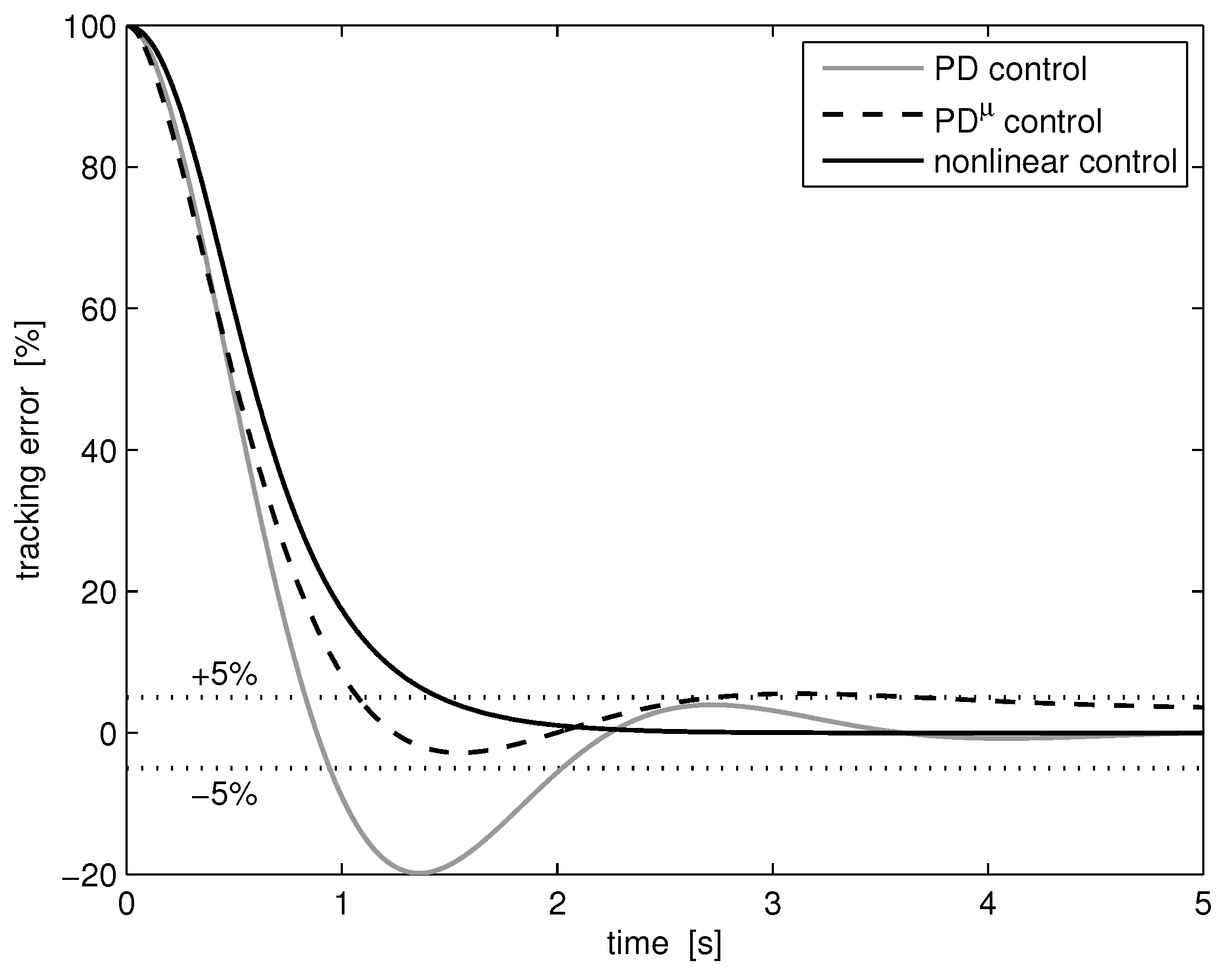
In order to quantify the performance level of the three closed-loop controller tested numerically, some metrics of the response of the closed-loop performance are provided in Table 3. The performance comparison can be made in terms of settling time, which is here measured as the time needed for the tracking error to be stabilized below $\pm 5\%$. As reported in Table 3, the fastest settling time is achieved by the nonlinear controller, while the slowest is the one obtained using the PD controller. Using a relative measurement of the settling time, the PD${}^{\mu }$ controller is 82% slower than the PD controller, while the nonlinear control is 28% faster than the PD controller. The time evolution of the percentage tracking error is shown in Figure 9.

Another measure of the closed-loop performances can be provided by the time needed to reduce the amplitude of the follower elastic vibration. In particular, Table 3 lists the time needed to reduce the amplitude of the elastic vibration below 1 × 10${}^{-4}$ m${}^{-1}$. With regards to this index, the best performance is obtained, again, by the nonlinear controller, which requires an 88% smaller time to reduce the vibration level below the chosen threshold in comparison with the PD controller. The PD${}^{\mu }$ controller allows a reduction of the same time over the PD controller equal to 42%. The best performance is obtained by the nonlinear controller also in terms of overshoot, which is equal to 0.006% for the nonlinear controller, 2.8% for the PD${}^{\mu }$ controller and 19.84% for the PD controller. The limited overshoot obtained by the use of the nonlinear controller can be explained by looking at the torque profile generated during the transient, which has a limited peak value. This feature is the main advantage brought by the derivative action included in the nonlinear formulation of the controller, which allows to set the proportional gain to a limited value. In this way, the overshoot is limited, since the bandwidth of the controller is kept high by a rather pronounced value of the $k_d$ gain, which in turn is compensated during the initial part of the transient by the negative value of the $k_n$ gain.

Table 3 lists also the peak value of the motor torque, obtained with the use of each control system. The measurements performed on the actuator action show that the nonlinear controller has a peak torque requirement that is equal to almost half of the peak torque needed when using the PD control. The peak torque produced by the PD${}^{\mu }$ controller is limited to 0.2 Nm in order to simulate the effects of an actuator with limited torque capabilities.

The choice of the tuning of the the three controls, whose values are shown in Table 2, has been performed using a trial-and-error procedure. Anyway, a possible procedure to establish a suitable tuning for the nonlinear control could be the following: first, the $k_n$ gain is set to zero, so as the nonlinear action is turned off. Then, a tuning procedure can be conducted using some well-known strategy, such as the Ziegler-Nichols formula [46]. Then, the obtained tuning can be refined by lowering the proportional gain $k_p$, increasing the derivative gain $k_d$, and introducing a small negative value for the $k_n$ gain. Before testing a new set of gains, the closed-loop stability should be checked using (16). This procedure has shown to produce good results, at least for second-order systems with lightly damped elastic modes, like the example presented in this work.

5. Conclusions

In this paper a novel nonlinear controller is proposed for the simultaneous position control and vibration damping in mechanisms with pronounced elasticity. The proposed method is model-free, and therefore its application does not require the explicit knowledge of the dynamic model of the plant to be controlled. Consequently, the proposed method is of simple and straightforward application, and is well suited to many industrial applications. An alternative formulation is provided for speed-controlled systems as well.

The conditions for the stability of the proposed nonlinear control are provided by the application Barbalat’s lemma to a suitable Lyapunov function candidate. The superior level of accuracy in terms of position tracking and vibration suppression achieved by the use of the nonlinear controller are shown by comparing it to a proportional-derivative control and a fractional order proportional-derivative control. The controls are applied to a challenging test case, i.e., the position and vibration control of a flexible four-bar linkage. The comparison with other controllers has highlighted a superior performance also in terms of improved settling time and of peak torque reduction.

References

- Benosman, M.; Le Vey, G. Control of flexible manipulators: A survey. Robotica 2004, 22, 533–545. [Google Scholar] [CrossRef]
- Korayem, M.H.; Nikoobin, A.; Azimirad, V. Trajectory optimization of flexible link manipulators in point-to-point motion. Robotica 2009, 27, 825–840. [Google Scholar] [CrossRef]
- Abe, A. An effective trajectory planning method for simultaneously suppressing residual vibration and energy consumption of flexible structures. Case Stud. Mech. Syst. Signal Process. 2016, 4, 19–27. [Google Scholar] [CrossRef] [Green Version]
- Zhang, X.; Xu, W.; Nair, S. Comparison of some modeling and control issues for a flexible two link manipulator. ISA Trans. 2004, 43, 509–525. [Google Scholar] [CrossRef]
- Benosman, M.; Boyer, F.; Le Vey, G.; Primault, D. Flexible links manipulators: From modelling to control. J. Intell. Robot. Syst. 2002, 34, 381–414. [Google Scholar] [CrossRef]
- Dwivedy, S.K.; Eberhard, P. Dynamic analysis of flexible manipulators, a literature review. Mech. Mach. Theory 2006, 41, 749–777. [Google Scholar] [CrossRef]
- Kiang, C.T.; Spowage, A.; Yoong, C.K. Review of Control and Sensor System of Flexible Manipulator. J. Intell. Robot. Syst. 2015, 77, 187–213. [Google Scholar] [CrossRef]
- Rahimi, H.; Nazemizadeh, M. Dynamic analysis and intelligent control techniques for flexible manipulators: A review. Adv. Robot. 2014, 28, 63–76. [Google Scholar] [CrossRef]
- Fung, R.F.; Chen, K.W. Dynamic analysis and vibration control of a flexible slider–crank mechanism using PM synchronous servo motor drive. J. Sound Vib. 1998, 214, 605–637. [Google Scholar] [CrossRef]
- Hill, D.E. Dynamics and control of a rigid and flexible four bar coupler. J. Vib. Control 2014, 20, 131–145. [Google Scholar] [CrossRef]
- Shin, H.; Rhim, S. Modeling and control of lateral vibration of an axially translating flexible link. J. Mech. Sci. Technol. 2015, 29, 191–198. [Google Scholar] [CrossRef]
- Garcia-Perez, O.; Silva-Navarro, G.; Peza-Solis, J. Flexible-link robots with combined trajectory tracking and vibration control. Appl. Math. Model. 2019, 70, 285–298. [Google Scholar] [CrossRef]
- Christoforou, E.G.; Damaren, C.J. The control of flexible-link robots manipulating large payloads: Theory and experiments. J. Robot. Syst. 2000, 17, 255–271. [Google Scholar] [CrossRef]
- Damaren, C.J. On the dynamics and control of flexible multibody systems with closed loops. Int. J. Robot. Res. 2000, 19, 238–253. [Google Scholar] [CrossRef]
- Chen, W. Dynamic modeling of multi-link flexible robotic manipulators. Comput. Struct. 2001, 79, 183–195. [Google Scholar] [CrossRef]
- Qin, H.; Li, Y.; Xiong, X. Workpiece pose optimization for milling with flexible-joint robots to improve quasi-static performance. Appl. Sci. 2019, 9, 1044. [Google Scholar] [CrossRef] [Green Version]
- Milford, R.; Asokanthan, S. Configuration dependent eigenfrequencies for a two-link flexible manipulator: Experimental verification. J. Sound Vib. 1999, 222, 191–207. [Google Scholar] [CrossRef]
- Giovagnoni, M.; Berti, G. A fractional derivative model for single-link mechanism vibration. Meccanica 1992, 27, 131–138. [Google Scholar] [CrossRef]
- Palomba, I.; Vidoni, R. Flexible-link multibody system eigenvalue analysis parameterized with respect to rigid-body motion. Appl. Sci. 2019, 9, 5156. [Google Scholar] [CrossRef] [Green Version]
- Elliott, J.; Dubay, R.; Mohany, A.; Hassan, M. Model Predictive Control of Vibration in a Two Flexible Link Manipulator-Part 1. J. Low Freq. Noise Vib. Act. Control 2014, 33, 455–468. [Google Scholar] [CrossRef]
- Elliott, J.; Dubay, R.; Mohany, A.; Hassan, M. Model Predictive Control of Vibration in a Two Flexible Link Manipulator-Part 2. J. Low Freq. Noise Vib. Act. Control 2014, 33, 469–484. [Google Scholar] [CrossRef] [Green Version]
- Bossi, L.; Rottenbacher, C.; Mimmi, G.; Magni, L. Multivariable predictive control for vibrating structures: An application. Control Eng. Pract. 2011, 19, 1087–1098. [Google Scholar] [CrossRef]
- Ioannou, P.A.; Sun, J. Robust Adaptive Control; Courier Dover Publications: New York, NY, USA, 2012. [Google Scholar]
- Caracciolo, R.; Richiedei, D.; Trevisani, A.; Zanotto, V. Robust mixed-norm position and vibration control of flexible link mechanisms. Mechatronics 2005, 15, 767–791. [Google Scholar] [CrossRef]
- Liao, W.H.; Chou, J.H.; Horng, I.R. Robust vibration control of flexible linkage mechanisms using piezoelectric films. Smart Mater. Struct. 1997, 6, 457. [Google Scholar] [CrossRef]
- Palomba, I.; Richiedei, D.; Trevisani, A. Reduced-order observers for nonlinear state estimation in flexible multibody systems. Shock Vib. 2018. [Google Scholar] [CrossRef]
- Singh, T.; Singhose, W. Input shaping/time delay control of maneuvering flexible structures. In Proceedings of the 2002 American Control Conference, Anchorage, AK, USA, 8–10 May 2002; Volume 3, pp. 1717–1731. [Google Scholar]
- Boscariol, P.; Gasparetto, A. Optimal trajectory planning for nonlinear systems: Robust and constrained solution. Robotica 2016, 34, 1243. [Google Scholar] [CrossRef]
- Giovagnoni, M. A numerical and experimental analysis of a chain of flexible bodies. J. Dyn. Syst. Meas. Control 1994, 116, 73–80. [Google Scholar] [CrossRef]
- Boscariol, P.; Gasparetto, A.; Zanotto, V. Active position and vibration control of a flexible links mechanism using model-based predictive control. J. Dyn. Syst. Meas. Control 2010, 132, 014506. [Google Scholar] [CrossRef]
- Caracciolo, R.; Richiedei, D.; Trevisani, A. Design and experimental validation of piecewise-linear state observers for flexible link mechanisms. Meccanica 2006, 41, 623–637. [Google Scholar] [CrossRef]
- Vidoni, R.; Gasparetto, A.; Giovagnoni, M. Design and implementation of an ERLS-based 3-D dynamic formulation for flexible-link robots. Robot. Comput. Integr. Manuf. 2013, 29, 273–282. [Google Scholar] [CrossRef]
- Vidoni, R.; Gallina, P.; Boscariol, P.; Gasparetto, A.; Giovagnoni, M. Modeling the vibration of spatial flexible mechanisms through an equivalent rigid-link system/component mode synthesis approach. J. Vib. Control 2017, 23, 1890–1907. [Google Scholar] [CrossRef]
- Vidoni, R.; Scalera, L.; Gasparetto, A. 3-D ERLS based dynamic formulation for flexible-link robots: Theoretical and numerical comparison between the finite element method and the component mode synthesis approaches. Int. J. Mech. Control 2018, 19, 39–50. [Google Scholar]
- De Luca, A.; Siciliano, B. An asymptotically stable joint PD controller for robot arms with flexible links under gravity. In Proceedings of the 31st IEEE Conference on Decision and Control, Tucson, AZ, USA, 16–18 December 1992; pp. 325–326. [Google Scholar]
- Armstrong, B.; Neevel, D.; Kusik, T. New results in NPID control: Tracking, integral control, friction compensation and experimental results. IEEE Trans. Control Syst. Technol. 2001, 9, 399–406. [Google Scholar] [CrossRef]
- Isidori, A. Nonlinear Control Systems; Springer Science & Business Media: Berlin/Heidelberg, Germany, 1995; Volume 1. [Google Scholar]
- Belanger, P.R.; Dobrovolny, P.; Helmy, A.; Zhang, X. Estimation of angular velocity and acceleration from shaft-encoder measurements. Int. J. Robot. Res. 1998, 17, 1225–1233. [Google Scholar] [CrossRef] [Green Version]
- Merry, R.; Van de Molengraft, M.; Steinbuch, M. Velocity and acceleration estimation for optical incremental encoders. Mechatronics 2010, 20, 20–26. [Google Scholar] [CrossRef] [Green Version]
- Petrella, R.; Tursini, M. An embedded system for position and speed measurement adopting incremental encoders. IEEE Trans. Ind. Appl. 2008, 44, 1436–1444. [Google Scholar] [CrossRef]
- Podlubny, I. Fractional-order systems and PIλDμ controllers. IEEE Trans. Autom. Control 1999, 44, 208–214. [Google Scholar] [CrossRef]
- Sabatier, J.; Agrawal, O.P.; Machado, J.T. Advances in Fractional Calculus; Springer: Berlin/Heidelberg, Germany, 2007; Volume 4. [Google Scholar]
- Tepljakov, A.; Petlenkov, E.; Belikov, J. FOMCON: A MATLAB toolbox for fractional-order system identification and control. Int. J. Microelectron. Comput. Sci. 2011, 2, 51–62. [Google Scholar]
- Chen, Y.; Petráš, I.; Xue, D. Fractional order control—A tutorial. In Proceedings of the American Control Conference, St. Louis, MO, USA, 10–12 June 2009; pp. 1397–1411. [Google Scholar]
- Oustaloup, A.; Levron, F.; Mathieu, B.; Nanot, F.M. Frequency-band complex noninteger differentiator: Characterization and synthesis. IEEE Trans. Circuits Syst. I Fundam. Theory Appl. 2000, 47, 25–39. [Google Scholar] [CrossRef]
- Hang, C.C.; Åström, K.J.; Ho, W.K. Refinements of the Ziegler–Nichols tuning formula. In IEE Proceedings D (Control Theory and Applications); IET: London, UK, 1991; Volume 138, pp. 111–118. [Google Scholar]
Figure 1.
Kinematic definitions of the ERLS.
Figure 2.
Four-bar linkage mechanism.
Figure 3.
Four-bar linkage: nodal elastic displacement and rigid displacement q.
Figure 4.
Angular position of the crank, comparison with PD and PD controllers.
Figure 5.
Curvature of the crank, comparison with PD and PD controllers.
Figure 6.
Curvature of the follower, comparison with PD and PD controllers.
Figure 7.
Curvature of the crank and follower, detail, comparison with PD controller.
Figure 8.
Motor torque, comparison with PD and PD controllers.
Figure 9.
Tracking error, percentage.