Incremental Canonical Correlation Analysis

Featured Application

This paper presents the solutions for real-time visual tasks such as visual tracking. Some real-life scenarios such as tracking specific targets can apply this method by extending ICCA.

Abstract

Canonical correlation analysis (CCA) is a kind of a simple yet effective multiview feature learning technique. In general, it learns separate subspaces for two views by maximizing their correlations. However, there still exist two restrictions to limit its applicability for large-scale datasets, such as videos: (1) sufficiently large memory requirements and (2) high-computation complexity for matrix inverse. To address these issues, we propose an incremental canonical correlation analysis (ICCA), which maintains in an adaptive manner a constant memory storage for both the mean and covariance matrices. More importantly, to avoid matrix inverse, we save overhead time by using sequential singular value decomposition (SVD), which is still efficient in case when the number of samples is sufficiently few. Driven by visual tracking, which tracks a specific target in a video sequence, we readily apply the proposed ICCA for this task through some essential modifications to evaluate its efficacy. Extensive experiments on several video sequences show the superiority of ICCA when compared to several classical trackers.

1. Introduction

Canonical correlation analysis, as a mathematical statistical tool, was proposed by Hovelling [1] in 1936. It is mainly used to analyze the association between two groups of random variables. In 2003, Hardoon et al. [2] briefly reviewed CCA and provided a generalized framework with optimization and kernel tricks. CCA is relevant to mutual information, thus it was used early in information retrieval. Later on, it was broadly applied to reduce dimension [3,4,5], clustering [6,7], regression [8,9], word embedding [10,11,12], and discriminant learning [13,14,15]. In such studies, plain CCA, which was purely used there, ignored the nonlinearity or geometrical structure within data sets. To this end, many variants of CCA emerged in diverse manners. For instance, sparse CCA [16] accounted for feature sparseness for more intuitive interpretation via $L_1$ regularization. Graph-embedded-based CCA (GCCA) [17,18,19] integrated local manifold structure within data for image classification by graph-embedded subspace learning with auxiliary methods [20,21]. More typically, deep CCA (DCCA) [22] trained the neural network under the guidance of the objective of CCA to model the data nonlinearity. In addition, generalized CCA (GCCA) [23] extended CCA with latent common feature representation. Similar to DCCA, deep GCCA [24] also realized CCA with deep architectures using the objective GCCA. In the above methods, eigenvalue decomposition, matrix inversion, or both are, as usual, involved. This obstructed the applicability of CCA and its variants in large-scale datasets or online learning tasks.

To make CCA efficient, many methods endeavored to explore efficient optimization algorithms, which address the computational inefficiency for the high-dimensional issue of CCA in different settings [25,26,27,28,29,30,31,32,33]. Kettenring et al. [34] showed that CCA was equivalent to the constrained least squares optimization problem. Zha et al. [35] calculated CCA by QR decomposition which denoted that a matrix $A$($A\in R^{m\times n}$) was divided into a product of an orthogonal matrix $Q$ and an upper triangular matrix $R$. However, the large scale of the data would still slow the calculation process. Afterwards, Avron et al. [36] proposed a fast CCA algorithm by employing randomized dimensionality reduction transform [37]. Recently, other methods to solve CCA were based on the methods of gradient descent. Ma et al. [33] introduced the enhanced approximate gradient mechanism and further extended it to stochastic optimization problems. In [38,39], CCA was reformulated into a series of least-square problems, which were solved by fast gradient descent. Such algorithms are still slow in reality. Thus, they are unsuited for online learning tasks.

To address this issue, we develop a simple yet efficient incremental canonical correlation analysis (ICCA) to accelerate plain CCA. Particularly, ICCA maintains constant memory storage for both the mean and covariance matrices, etc., in an adaptive manner. This does not require storage of large amounts of history data, thus a certain space complexity remains. To reduce time complexity, we readily avoid matrix inverse in the learning process by using sequential Karhunen–Loeve (SKL) or singular value decomposition (SVD), which is still efficient in the case that the number of samples is sufficiently few. Driven by visual tracking as an online learning task, which locates a given target in a long video sequence, we apply the proposed ICCA for this task through some essential modifications to ensure its efficacy. Extensive experiments on several video sequences show the superiority of ICCA as compared to several classical trackers. Importantly, the efficiency of ICCA is promising.

There are three aspects to our contribution: (1) we provide a new perspective to solve the efficiency problem of CCA; (2) from the perspective of SVD, we propose an ICCA method to avoid the invert matrix multiplication for saving overhead time; and (3) a tracking algorithm based on ICCA further tries to expand the applicability of CCA for real-life scenarios.

The rest of this paper is outlined as follows. We list the related work about CCA in Section 2. Section 3 details CCA and our method. Section 4 offers the experimental results, and we give our conclusions in Section 5.

2. Related Work

Owing to the problem of CCA described above, a large number of methods were proposed to solve this problem. Most studies were along the specific application of this main line to improve CCA. Based on this consideration, we mainly review in this section those optimization algorithms about CCA that are most related to our method.

To accelerate the efficiency of CCA, a randomized CCA algorithm for a pair of tall and thin matrices was proposed in [36], which first obtained the matrices by randomly reducing the dimensionality of the matrices. The newly generated matrices, as a different dataset, were applied in existing algorithms. As a result, Ma et al. [33] pinpointed that the randomized CCA algorithm still cannot thoroughly solve the original high complexity problems. Lu et al. [31] obtained some suboptimal results by viewing this problem as a sequence of iterative least-squares with imprecise approximation. An iterative algorithm achieved excellent results with a low cost. In [30], an alternating least-squares algorithm was proposed and the performance is better than [33]. Gao et al. [29] found that the objective of CCA is not stochastic convex programming. Ma et al. [33] gave much attention to globally convergent stochastic optimization of CCA. Ge et al. [39] made a breakthrough to this issue. However, the problem of sample complexity still exists. Xu et al. [40] proposed truly alternating least-squares (TALS) for efficient CCA with momentum. The offline algorithm was not suitable for real-time scenes that resulted in high memory storage, so some scholars tried to design fast algorithms to solve the problem of high complexity. Marinov et al. [29] proposed a first-order stochastic approximation algorithm for canonical correlation analysis (CCA), in which the convex relaxation was introduced. Different from these methods, which all approximated the objective of plain CCA, the proposed ICCA directly accelerates original CCA. Note that the sequential Karhunen–Loeve or SVD used in ICCA was originally proposed by Kim [41], which accelerated SVD rather than matrix inversion. Moreover, early on, it was applied in visual tracking [42], which puts forward learning the eigenbasis of PCA. It is obvious that PCA is not CCA and their motivations are very different. More importantly, the proposed ICCA greatly expands the applicability of sequential SVD in multiview tasks.

3. Methodology

3.1. Review of Canonical Correlation Analysis

Canonical correlation analysis (CCA) as a classical multivariate statistical method is widely used to analyze multiview data. In the machine learning community, CCA usually serves as a feature learning method of extracting two separate subspaces to maximize the correlations across views. Consider the samples $X\in R^{d_1\times n}$ and $Y\in R^{d_2\times n}$ from two views, where $d_1$ and $d_2$ are respectively the dimensions of $X$ and $Y$, and $n$ denotes the number of the samples; CCA [43] is to seek two subspaces $a$ and $b$ to maximize their projections, as given below:

$$\underset{a,b}{\max }\frac{a^T{\mathsf{\Sigma }}_{xy}b}{\sqrt{a^T{\mathsf{\Sigma }}_{xx}a}\sqrt{b^T{\mathsf{\Sigma }}_{yy}b}}$$

(1)

where ${\mathsf{\Sigma }}_{xy}=(X-\overline{X}){(Y-\overline{Y})}^T$, ${\mathsf{\Sigma }}_{xx}=(X-\overline{X}){(X-\overline{X})}^T$, ${\mathsf{\Sigma }}_{yy}=(Y-\overline{Y}){(Y-\overline{Y})}^T$.

To ensure the scale invariance of $a$ and $b$ in Equation (1), the objective function can be rewritten:

$$\begin{array}{l}\underset{a,b}{\max }{a}^T{\mathsf{\Sigma }}_{xy}b\\ s.t.a^T{\mathsf{\Sigma }}_{xx}a=1\\ b^T{\mathsf{\Sigma }}_{yy}b=1\end{array}$$

(2)

By constructing a Lagrange equation, Equation (2) is simplified into:

$$\left[\begin{array}{cc}{\mathsf{\Sigma }}_{xx}^{-1}& 0\\ 0& {\mathsf{\Sigma }}_{yy}^{-1}\end{array}\right]\left[\begin{array}{cc}0& {\mathsf{\Sigma }}_{xy}\\ {\mathsf{\Sigma }}_{yx}& 0\end{array}\right]\left[\begin{array}{c}a\\ b\end{array}\right]=\lambda \left[\begin{array}{c}a\\ b\end{array}\right]$$

(3)

It is proved that the Equation (3) has a global optimal solution, in which $a$ and $b$ are called as canonical subspaces. Before computing $a$ and $b$, ${\mathsf{\Sigma }}_{xx}^{-1}$, ${\mathsf{\Sigma }}_{yy}^{-1}$, ${\mathsf{\Sigma }}_{xy}$, and ${\mathsf{\Sigma }}_{yx}$ should be calculated at first. However, the time complexity of the matrix inversion about ${\mathsf{\Sigma }}_{xx}^{-1}$ and ${\mathsf{\Sigma }}_{yy}^{-1}$ is $O(d^3)$ ($d$ is the larger of the two $d_1$ and $d_2$), which leads to slow running speed and large calculation overhead [2,40,41]. In practice, there are many data with high dimensions that burden massive data storage. Obviously, using CCA incremental learning is a promising choice to handle this case.

3.2. Incremental Canonical Correlation Analysis (ICCA)

Mean and Covariance Update. In CCA, calculating the mean and covariance is a necessary step for its solution. For the mean and covariance update, it is relatively easy to keep the storage constant. For completeness, we introduce the concrete strategy, where the implementation details could not be slightly different from other methods. Suppose that there are $n$ old samples and $m$ new incoming samples. Let $\overline{X}$ and $\overline{Y}$ denote the mean of $n$ old samples from $X$ and $Y$, respectively. Correspondingly, the covariance of $n$ old samples and $m$ new incoming samples between $X$ and $Y$ sample are denoted by ${\mathsf{\Sigma }}_{xy}$ and ${\mathsf{\Sigma }}_{xy}^{\prime }$, respectively. ${\mathsf{\Sigma }}_{xy}^{″}$ denotes the covariance of $n^t$ samples.

$${\mathsf{\Sigma }}_{xy}^{″}=\frac{m-1}{n^t}{\mathsf{\Sigma }}_{xy}+\frac{m-1}{n^t-1}{\mathsf{\Sigma }}_{xy}^{\prime }+\frac{m(m+n^t)}{(n^t-1)n^t}(\overline{X^{\prime }}-X){(\overline{Y^{\prime }}-Y)}^T$$

(4)

where

$$\begin{array}{l}{\mathsf{\Sigma }}_{xy}={\displaystyle \sum _{i=1}^n(X_i-\overline{X})}{(Y_i-\overline{Y})}^T,\\ {\mathsf{\Sigma }}_{xy}^{\prime }={\displaystyle \sum _{i=n+1}^{n+m}(X_i-\overline{X})}{(Y_i-\overline{Y})}^T,\\ \overline{X}={\displaystyle \sum _{i=1}^n{X}_i},\overline{Y}={\displaystyle \sum _{i=1}^n{Y}_i},\\ \overline{X^{\prime }}={\displaystyle \sum _{i=n+1}^{n+m}{X}_i},\overline{Y^{\prime }}={\displaystyle \sum _{i=n+1}^{n+m}{Y}_i},\\ n^t=fn+m\end{array}$$

(5)

and $f$ denotes a forgotten factor to eliminate old samples, $f\in [0,1]$. The parameter $f=1$ expresses that more emphasis is put on all the samples, while $f=0$ indicates that a full focus is placed on the new samples.

The $n$ previous history matrices including ${\mathsf{\Sigma }}_{xy}$, $\overline{X}$ and $\overline{Y}$ need to be saved before $m$ new samples arrive. The matrix ${\mathsf{\Sigma }}_{xy}^{\prime }$, $\overline{X^{\prime }}$ and $\overline{Y^{\prime }}$ can be obtained with the new $m$ samples and then the covariance of matrix ${\mathsf{\Sigma }}_{xy}^{″}$ can be calculated, based on these $n$ old samples and $m$ new incoming samples. Thus, all the samples do not take up much memory. Of them, the mean of all the samples at this time can be updated as follows:

$$\begin{array}{l}{\overline{X}}_{n+m}=\frac{n}{n^t}·\overline{X}+\frac{n}{n^t}\overline{X^{\prime }}\\ {\overline{Y}}_{n+m}=\frac{n}{n^t}·\overline{Y}+\frac{n}{n^t}\overline{Y^{\prime }}\end{array}$$

(6)

when the next $m$ samples emerge again, once the matrix ${\mathsf{\Sigma }}_{xy}^{″}$, $\overline{X}$, and $\overline{Y}$ are computed according to Equation (5), the saved value of $n^t$ and the historical matrix ${\mathsf{\Sigma }}_{xy}$ directly take part in the new round of calculation and storage. The complete operation would not increase the storage space with the rapid of the number of samples.

Avoiding Matrix Inversion. To solve CCA, it is necessary to solve the inversion of matrix ${\mathsf{\Sigma }}_{xx}$ and ${\mathsf{\Sigma }}_{yy}$ in Equation (3). To avoid the matrix inversion, we resort to the singular value decomposition (SVD), which efficiently solves the thinner matrix. Given any matrix $A\in R^{d\times n}$, its SVD form is as follows:

$$A\stackrel{SVD}{=}US{V}^T$$

(7)

where $U\in R^{d\times d}$, $S\in R^{d\times n}$, $V\in R^{n\times n}$; then $A{A}^T=US{V}^{T}VS{U}^T$. Owing to the orthogonality $V{V}^T=I$, and thus $A{A}^T=USS{U}^T$. When $X-\overline{X}=U_1{S}_1{V}_1^T$, ${\mathsf{\Sigma }}_{xx}$ is a real symmetric matrix and thus

$${\mathsf{\Sigma }}_{xx}^{-1}={({\mathsf{\Sigma }}_{xx}^T)}^{-1}={(U_1{S}_1^2{U}_1^T)}^{-1}=U_1{S}_1^{-2}{U}_1^T$$

(8)

In Equation (8), there is an inverse operation $S_1^{-2}$. Since $S_1$ is a diagonal matrix whose elements are only located on the diagonal, its inversion can be calculated by the reciprocal of each element. Likewise, ${\mathsf{\Sigma }}_{yy}^{-1}={({\mathsf{\Sigma }}_{yy}^T)}^{-1}={(U_2{S}_2^2{U}_2^T)}^{-1}=U_2{S}_2^{-2}{U}_2^T$. $S_2^{-2}$ can be obtained the same as $S_1^{-2}$. So, the matrix inverse is avoided.

It is obvious that the overhead of vanilla SVD is not ignored as well, if the matrix is still relatively large. Towards this end, a sequential Karhunen–Loeve algorithm (SKL) [44] can be employed here. Without loss of generality, suppose that $n$ centralized samples $X$ and the m new centered incoming samples $X^{\prime }$. Assume that $X=U_1{S}_1{V}_1^T$. Obviously, the SVD of the concatenation $X$ and $X^{\prime }$ is $\left[X{X}^{\prime }\right]=U_1^{\prime }{\mathsf{\Sigma }}_1^{\prime }{V}_1^{\prime }{}^T$. Let $X^{″}$ be the component of $X^{\prime }$ orthogonal to $U_1$, $U^{\prime }=[U_1,X^{″}]$, and $V^{\prime }=\left[\begin{array}{cc}{V}_1^{\prime }& 0\\ 0& I_m\end{array}\right]$, where $I_m$ is the identity matrix with the size of $m$. Then, we derive a small matrix $X_n=U^{\prime }\left[X,X^{\prime }\right]V^{\prime T}$. The SVD of $X_n$ is $X_n=\tilde{U}\tilde{D}{\tilde{V}}^T$, then $\left[X,X^{\prime }\right]=U^{\prime }\tilde{U}\tilde{D}{\tilde{V}}^T{V}^{\prime }{}^T$. Obviously, we need the latest left singular matrix $U_1^{\prime }=U^{\prime }\tilde{U}$ and the corresponding singular value matrix ${\mathsf{\Sigma }}_1^{\prime }=\tilde{D}$. Now we can obtain the inverse of the covariance matrix of $X$.

Adopting the SKL algorithm [44] can ensure its space and time complexity to be constant in $O(n+m)$. Each update only adopts the first top $k-$ truncated singular value and basis vectors in the former step and the $m$ new incoming samples, thus the space complexity is reduced to $O(d(k+m))$ instead of the previous $O(d{(n+m)}^2)$ as in Levy and Lindenbaum [44].

Updating Subspaces. Of course, the SKL algorithm is designed for sequential SVD methods. Thus, we follow the section above to find the SVD of ${\mathsf{\Sigma }}_{xy}$. Since merging the small-sized matrices into the SVD forms of ${\mathsf{\Sigma }}_{xx}^{-1}$, ${\mathsf{\Sigma }}_{yy}^{-1}$, and ${\mathsf{\Sigma }}_{xy}$, we can efficiently obtain the SVD of $P={\mathsf{\Sigma }}_{xx}^{-1/2}{\mathsf{\Sigma }}_{xy}{\mathsf{\Sigma }}_{yy}^{-1/2}$. In fact, we do not need the concrete form. This is because the projection matrix only requires the left and right singular matrices. The update formula is

$$\{\begin{array}{c}a={\mathsf{\Sigma }}_{xx}^{-1/2}u\\ b={\mathsf{\Sigma }}_{yy}^{-1/2}v\end{array}$$

(9)

where $u$ and $v$ are the left and right singular matrices of $P$, respectively. Here, the subspace $a$ and $b$ can be updated.

The specific optimization algorithm is shown in Algorithm 1.

4. Experiments

In this section, we apply ICCA for visual tracking with particle filter to illustrate the applicability of incremental CCA (ICCA).

4.1. Settings

Implementation Details. For completeness, following the experimental settings [41], we divide an image into left and right patches. Since occlusion and illumination affects the tracking results, we at the meantime extend the method of [45] to the case of two views. In detail, we directly extract the projection matrices of two views as the bases, which serve as the templates. To integrate two views of templates into the particle filtering framework, we utilize the reconstruction errors to determine the best candidate as the position inference. Different from [45], the updating reconstructed coefficients rely on the templates from two views rather than independent views. For clarity, we give the concrete details as Equation (10):

Algorithm 1. Incremental Subspace Algorithm

Input:$n$ samples $X$ and $Y$, $m$ new samples $X^{\prime }$ and $Y^{\prime }$.

Output: the updated subspace $New\_U_1$, $New\_U_2$ the updated mean and covariance ${\overline{X}}_{n+m}$,${\overline{Y}}_{n+m}$, ${\tilde{\mathsf{\Sigma }}}_{xy}$;

1. Update the mean $\overline{X}$, $\overline{Y}$ and covariance ${\mathsf{\Sigma }}_{xy}$ and ${\mathsf{\Sigma }}_{yx}$ of $n$ samples, according to Equation (5);

2. Update the mean ${\overline{X}}_{n+m}$, ${\overline{Y}}_{n+m}$ of $n+m$ current samples according to Equation (6);

3. $\overline{X}\leftarrow {\overline{X}}_{n+m},\overline{Y}\leftarrow {\overline{Y}}_{n+m},{\tilde{\mathsf{\Sigma }}}_{xy}\leftarrow {\mathsf{\Sigma }}_{xy}$ according to Equations (4) and (5);

4. Calculate $U_1$, $S_1$, $U_2$, and $S_2$ according to Equation (7);

5. Calculate ${\mathsf{\Sigma }}_{xx}^{-1},{\mathsf{\Sigma }}_{yy}^{-1}$ according to Equation (8);

6. Calculate $a$ and $b$ to yield new subspace $New\_U_1$, $New\_U_2$ according to Equation (9).

$$\underset{\alpha ,e_1,e_2}{\min }\frac{1}{2}{\Vert x-D_1\alpha -e_1\Vert }_F^2+\frac{1}{2}{\Vert y-D_2\alpha -e_2\Vert }_F^2+{\mu }_1{\Vert e_1\Vert }_1+{\mu }_2{\Vert e_2\Vert }_2+\lambda {\Vert \alpha \Vert }_0$$

(10)

where $x$ and $y$ denote the left and right patches, respectively, $D_1$ and $D_2$ denote the projection matrices learned by ICCA, $\alpha$ is the sparse coefficient vector, $e_1$ and $e_2$ denote the noises, and $\lambda$, ${\mu }_1$, and ${\mu }_2$ denote the regularization parameters.

According to [45], we ignore the same solution steps such as the errors $e_1$ and $e_2$, and only describe the reconstructed coefficient update rule. Since the iterative shrinkage technique requires the partial derivative about the coefficient, the first step is to calculate the partial derivative of Equation (10) with respect to $\alpha$. Let $G_a$ is the objective function about $\alpha$ after simplification:

$$G_{\alpha }=\frac{1}{2}{\Vert D_1^T(x-e_1)-D_1^T{D}_1\alpha \Vert }_F^2+\frac{1}{2}{\Vert D_2^T(y-e_2)-D_2^T{D}_2\alpha \Vert }_F^2$$

(11)

Then the gradient about $\alpha$ is:

$$\frac{\partial G_{\alpha }}{\partial \alpha }={(D_1^T{D}_1+D_2^T{D}_2)}^{-1}(D_1^T(x-e_1)-D_2^T(y-e_2))$$

(12)

Similarly, the gradient about $e_1$ and $e_2$ is $e_1-(x-D_1\alpha )$ and $e_2-(y-D_2\alpha )$. With the three gradients, $\alpha$, $e_1$, and $e_2$ can be obtained by combination with APG (accelerated proximal gradient).

In visual tracking with a particle filter, one particle with maximum probability must be chosen as the target location in the next-coming frame. According to Bayesian theory, the maximum probability of particles is expressed as follows:

$$p(X_i,Y_i|S_m)=\exp (-J({\alpha }^{*},e_1^{*},e_2^{*}))$$

(13)

where $J(\alpha ,e_1,e_2)=\frac{1}{2}{\Vert x-D_1\alpha -e_1\Vert }_F^2+\frac{1}{2}{\Vert y-D_2\alpha -e_2\Vert }_F^2+{\mu }_1{\Vert e_1\Vert }_1+{\mu }_2{\Vert e_2\Vert }_1$, ${\alpha }^{*}$, $e_1^{*}$, $e_2^{*}$ are the optimal solution of Equation (10). $S_m$ represents the particle state in the $m$-th frame. These states are composed of six affine parameters and are estimated with the maximum posteriori probability. The maximum probability particle is calculated and treated as the target location in the next frame.

In order to ensure the fairness of comparison and the reliability of the experiment, the running environment of all video frames is performed on the same workstation. In order to fully mine multimode features, the ICCA tracker uses two parts of each particle evenly divided horizontally or vertically as two view features. In the experiment, the regularization parameters of ICCA tracker are set: $\lambda$ is selected from {0.005, 0.05, 0.06, 0.25, 0.1}, ${\mu }_1$ is selected from {0.06, 0.08, 0.09, 0.1, 0.15, 0.25, 0.35, 0.3}, and ${\mu }_2$ is selected from {0.06, 0.08, 0.09, 0.1, 0.15, 0.25, 0.35, 0.3}.

Datasets. This section compares ICCA with several representative trackers, such as robust fragments-based tracking (Frag) [46], visual tracking decomposition (VTD) [47], incremental learning for robust visual tracking (IVT) [42], real time robust L1 tracker using accelerated proximal gradient approach (L1APG) [48], visual tracking with online multiple instance learning (MIL) [49], correlation-based incremental visual tracking (TLD) [41] on a series of video sequences, including basketball, car4, cardark, carscale, deer, Dudek, faceocc1, fish, football, and 18 other video sequences to verify the effectiveness of ICCA. Of the trackers compared, VTD selects multiple image feature models and motion models at the same time, and tracks them respectively. Finally, the optimal feature and motion model are combined as the optimal target area in real time; IVT is a video tracking algorithm based on the incremental update appearance model and maintains a template in the whole tracking process, and dynamically updates the template through incremental PCA, so that it can effectively adapt to changes in appearance. L1APG is based on sparse representation and uses accelerated proximal gradient (APG) to solve the L1 minimization problem. The MIL tracker treats the visual tracking problem as the multi-instance learning problem, in which the bag is composed of many instances instead of a single instance. TLD combines the traditional tracking algorithm and detection algorithm to solve the problems of deformation and occlusion in tracking. Frag is recognized by partial matching. Its target template is described by multiple fragments and blocks of the image. Blocks are arbitrary, not based on the target model. These trackers used here represent different types of trackers and are the most representative shallow learning trackers, which are widely used for comparison purposes in research reports. More importantly, such main tracking algorithms are integrated into a tracking framework [50], which provides the evaluation and figure codes for fair comparison. This paper also implements the ICCA algorithm on the basis of this tracking framework. The video sequences used here, which include different appearance changes of tracking objects in different scenes, can be downloaded from this tracking framework as well.

4.2. Results

In single object tracking, two evaluation criteria are mainly used: qualitative analysis and quantitative analysis. In a video sequence, the tracking effect belongs to the category of qualitative analysis. To track the target, whether the tracking is lost from the first frame to the last frame, and whether the target tracking frame can dynamically follow the change of target size is qualitative analysis. In addition, precision and success rate are used for quantitative analysis. The traditional method to evaluate the tracker is to take the real position of the tracking target in the first frame as the initial tracking target in the test set, and calculate the average accuracy or success rate through the whole test sequence. This is a one-way evaluation (OPE). In addition to these evaluation criteria, we also report the efficiency of each algorithm in terms of the number of frames per second (FPS).

4.2.1. Efficiency Comparison

In

Table 1. The FPS of the compared trackers on eighteen videos.

	ICCA	IVT	L1APG	TLD	VTD	MIL	Frag
Basketball	31.01	22.09	2.36	19.81	13.36	30.6	2.74
Car4	30.8	22.1	1.6747	14.97	8.26	27.73	7.07
Cardark	33.12	32.41	3.27	25.22	18.95	27.16	6.68
Carscale	25.01	22.23	2.59	23.79	12.96	24.66	3.47
David3	32.71	31.65	3.01	19.65	14.10	25.45	3.19
Deer	23.7	21.9	2.1516	16.62	12.15	17.38	2.68
Faceocc1	28.87	27.31	4.56	17.85	13.80	27.78	4.27
Faceocc2	30.95	22.49	3	21.93	13.80	29.01	5.32
Fish	37.05	29.01	2.22	36.11	16.48	25.02	5.39
Football	31.53	22.06	3.44	20.99	13.67	31.56	2.87
Crossing	34.12	27.84	1.48	30.14	12.96	11.6	4.89
Dog1	23.03	22.86	1.66	10.03	8.44	18.67	6.71
Jogging-2	26.81	5.3	0.18	26.71	19.82	30.06	5.36
Jumping	29.76	8.53	1.02	10.78	14.87	29.8	7.41
Mhyang	31.34	7.31	3.17	12.09	7.76	46.3	3.15
Mountain Bike	32.36	31.96	3.02	17.98	14.27	27.93	3.67
Singer1	35.79	22.49	2.29	23.19	14.49	34.56	3.44
Walking	33.08	32.22	4.34	12.45	13.52	28.34	2.19

, we offer the FPS values of the compared trackers on all eighteen videos, which are computed as the ratio of the total number of frames in each video length to the total running time, namely, the number of frames per second based on various tracking methods. The larger the value, the higher the efficiency of the tracking algorithm. As in Table 1, ICCA achieves larger values of FPS on most videos. In some videos, like football, jumping, and mhyang, the changes in appearances make the tracking difficult, which leads to the slower convergence of the tracking algorithm based on our ICCA with the same criterion used on the other videos. Thus, the values of FPS are not always the best.

4.2.2. Qualitative Comparison

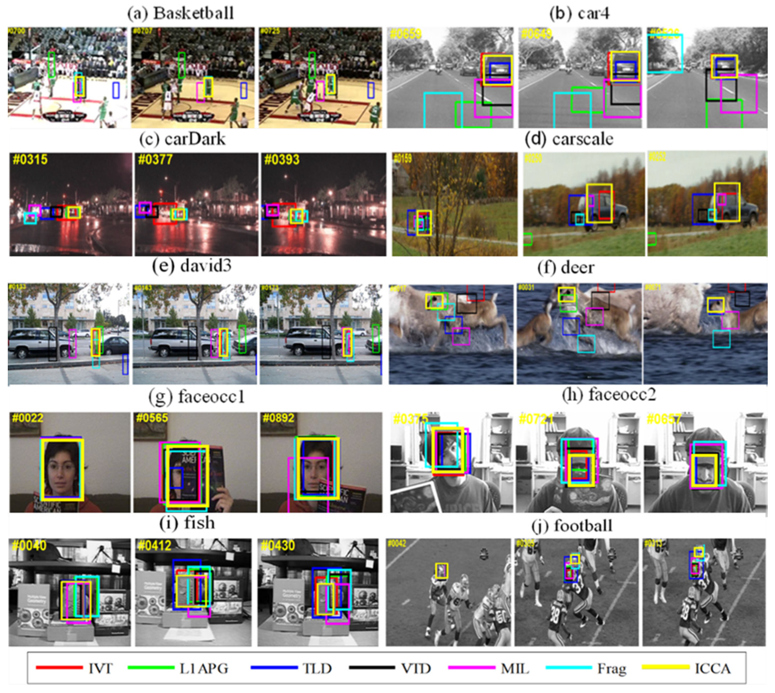
In the basketball and football videos, the target is a fast-moving person. For the basketball video, when more than one player grabs the ball, the tracking player is easily affected by the background information. In the football video, in addition to being easily affected by the background information, the helmet information is similar, when the players occlude each other, and the tracked target is easy to lose.

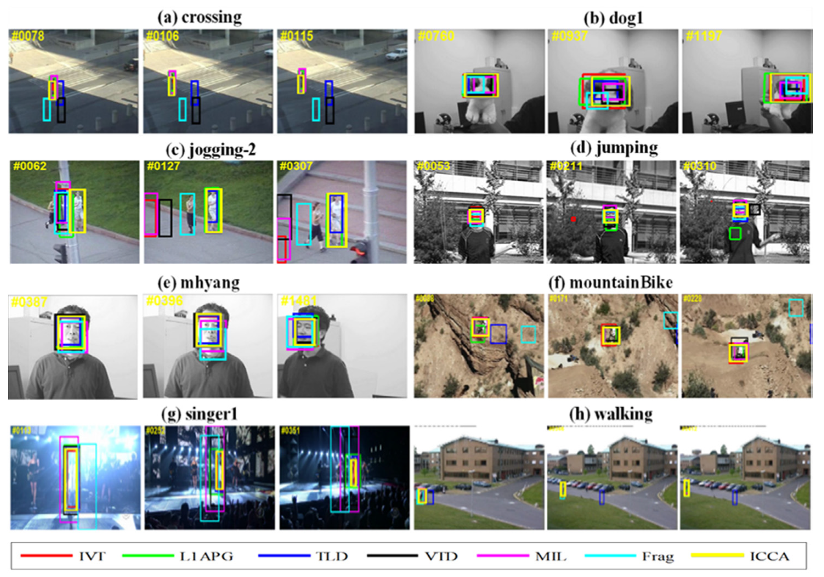
Figure 1a,j show good tracking ability of ICCA, which is better than other trackers in the football video. In the three videos of car4, cardark, and carscale, fast-moving cars drive on the streets during the day and night, as well as on the outdoor roads during the day. For the video car4, when the car passes through the overpass or under the shade of trees, its surface light changes greatly. In the video cardark, cars on the street at night are easily blurred by the brightness of other lights or street lights. The car in the video carscale will drive from far to near, and the scale will change when passing through a cluster of branches. Figure 1b–d shows that ICCA tracking results are attractive. In Figure 1e, namely, the video david3, the tracked person walks outdoors. In the process of walking back and forth, it is occluded twice by the trunk. Most tracking algorithms lose the target, while ICCA still works stably. In the deer video sequences, most algorithms fail because the tracked deer is very similar to the surrounding background and moves rapidly; ICCA effectively performs the tracking. The dog in the video Dog1 moves from near to far but slowly, thus most methods can track the target stably. As in Figure 1, the videos faceocc1, faceocc2, and jogging-2 share the common things: the tracked targets are all sometimes occluded, especially the target in jogging-2 has almost complete occlusion, and the color of the occlusion appearance is very similar to the target. ICCA works well and shows its effectiveness. In the video fish, because the camera is shaking slightly, it is more difficult to track the target. ICCA can track the target accurately. In Figure 2a, since the building in the video crossing blocks the sun, the pedestrian tracking is relatively stable in the building shadow. When walking to the shadow and direct light, illumination variations are quite different. In this case, most trackers miss the target, but ICCA can still track the target even when the tracking bounding box size changes a little. In the singer1 video, the background clutter affects the effective learning of the subspace. Likewise, ICCA can track the target correctly.

4.2.3. Quantitative Comparison

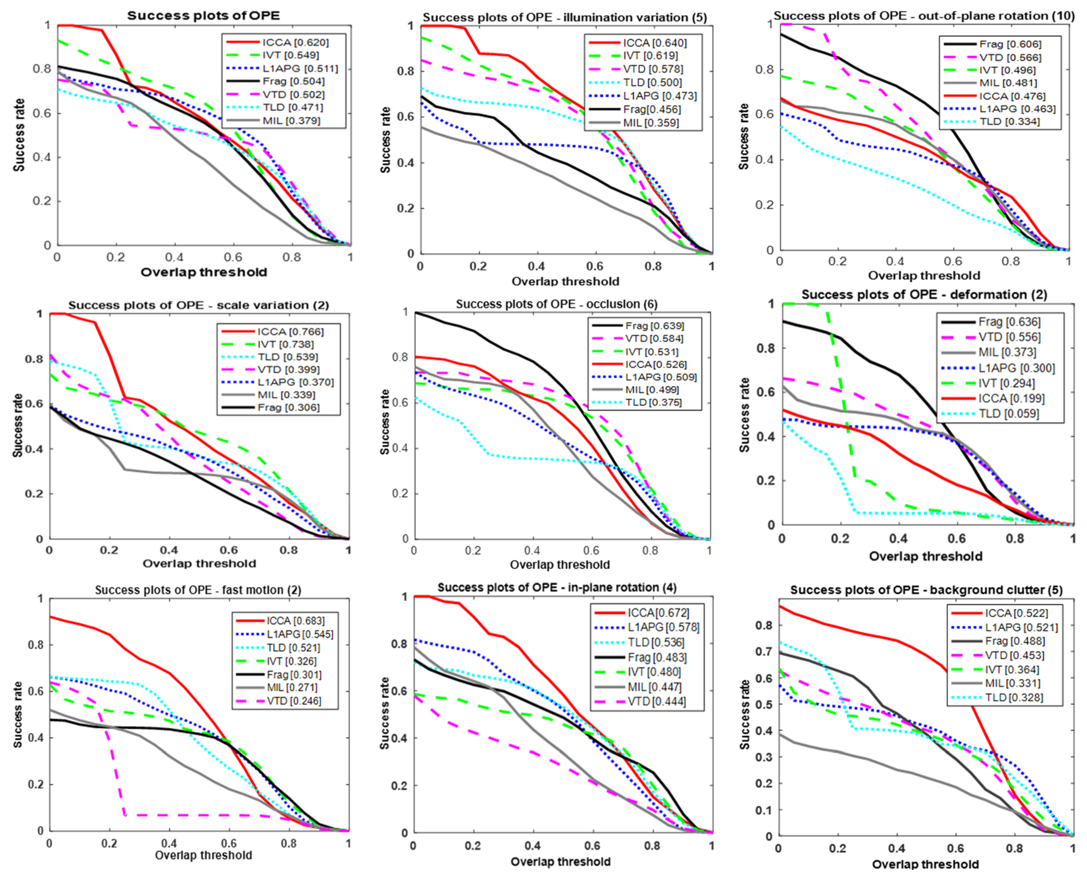
To quantify the visual tracking performance of ICCA, seven trackers were evaluated and compared by success rate and precision. It can be seen from Figure 3 that ICCA has almost the best comprehensive performance, and has a high success rate on different attributes, such as background speckle illumination, scale change, rapid movement, and small rotation of objects, but it achieves slightly worse performance than other trackers on out-of-plane rotation, occlusion, and deformation.

In particular, ICCA merely depends on the subspace learning, which as usual is not very robust. ICCA mainly accelerates CCA in an incremental way, in which the solution to CCA is a closed-form rather than stochastic approximation. In addition, ICCA primarily focuses on the efficiency and applicability in real scenarios.

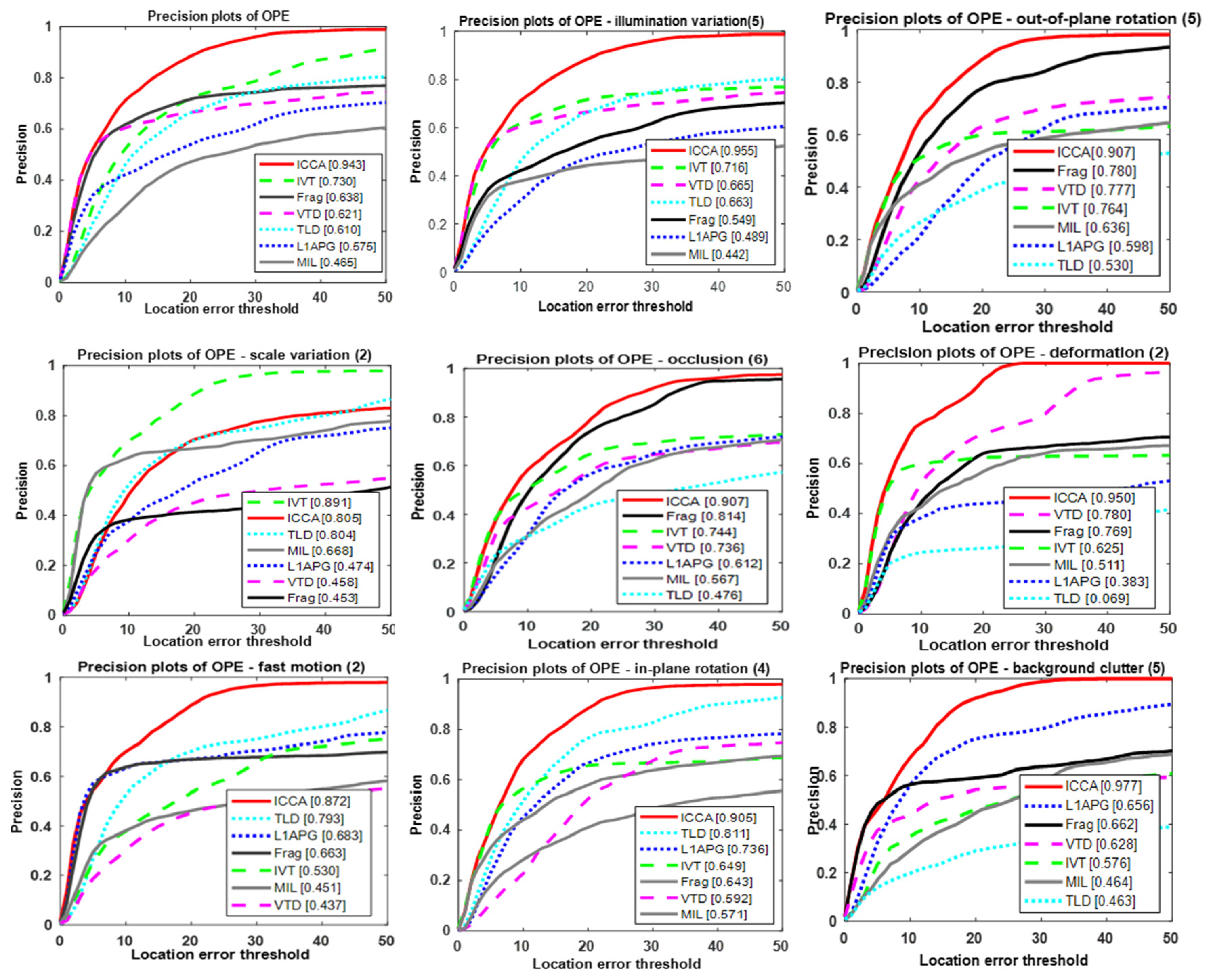
Figure 4 shows the precision comparison of seven trackers over 18 video sequences. ICCA is consistently superior to other trackers for high accuracy on most attributes. Since ICCA just accelerates CCA without improving the robustness of target appearance, the trackers based on ICCA are still sensitive to the occlusion, scale size, and deformation. Thus, on such attributes, the performance based on ICCA is slightly lower than other trackers. We cannot guarantee our tracker to work on all the videos because we only improve the efficiency of CCA rather than its model capacity.

In short, according to the comparison of success rate and accuracy, the ICCA tracker is better than other previous trackers and exhibits better performance on many video sequences.

5. Conclusions

This paper details a simple yet efficient incremental CCA (ICCA), and applies it for visual tracking to verify the effectiveness and promising potential for proposed online learning schemes in reality. Different from existing works, the proposed ICCA directly accelerates the process of CCA, in contrast to some other approximations. The algorithmic efficiency is greatly improved. However, it still needs to develop other applications for further in-depth analysis.

References

- Harold, H. Relations between two Sets of Variables. Biometrika 1936, 28, 3–4. [Google Scholar]
- Hardoon, D.; Szedmak, S.; Shawe-Taylor, J. Canonical Correlation Analysis: An Overview with Application to Learning Methods. Neural Comput. 2004, 16, 2639–2664. [Google Scholar] [CrossRef] [Green Version]
- Sun, L.; Ceran, B.; Ye, J.P. A scalable two-stage approach for a class of dimensionality reduction techniques. In Proceedings of the 16th ACM SIGKDD International Conference on Knowledge Discovery and Data Mining, Washington, DC, USA, 25–28 July 2010. [Google Scholar]
- Yuan, Y.H.; Sun, Q.S.; Ge, H.W. Fractional-order embedding canonical correlation analysis and its applications to multi-view dimensionality reduction and recognition. Pattern Recognit. 2014, 47, 1411–1424. [Google Scholar] [CrossRef]
- Zhang, Y.; Zhang, J.; Pan, Z.; Zhang, D. Multi-view dimensionality reduction via canonical random correlation analysis. Front. Comput. Sci. 2016, 10, 856–869. [Google Scholar] [CrossRef]
- Blaschko, M.B.; Lampert, C.H. Correlational spectral clustering. In Proceedings of the IEEE Conference on Computer Vision and Pattern Recognition, Anchorage, AK, USA, 23–28 July 2008; pp. 1–8. [Google Scholar]
- Chaudhuri, K.; Kakade, S.M.; Livescu, K.; Sridharan, K. Multi-view clustering via canonical correlation analysis. In Proceedings of the 26th Annual International Conference on Machine Learning, Montreal, QC, Canada, 14–18 June 2009. [Google Scholar]
- Kakade, S.M.; Foster, D.P. Multi-view Regression Via Canonical Correlation Analysis. In International Conference on Computational Learning Theory; Bshouty, N.H., Gentile, C., Eds.; Springer: Berlin/Heidelberg, Germany, 2007. [Google Scholar]
- Lambert, Z.V.; Wildt, A.R.; Durand, R.M. Redundancy analysis: An alternative to canonical correlation and multivariate multiple regression in exploring interset associations. Psychol. Bull. 1988, 104, 282–289. [Google Scholar] [CrossRef]
- Dhillon, P.; Rodu, J.; Foster, D.; Ungar, L. Two Step CCA: A new spectral method for estimating vector models of words. Comput. Sci. 2012, 2, 67–74. [Google Scholar]
- Gong, Y.; Ke, Q.; Isard, M.; Lazebnik, S. A Multi-View Embedding Space for Modeling Internet Images, Tags, and Their Semantics. Int. J. Comput. Vis. 2014, 106, 210–233. [Google Scholar] [CrossRef] [Green Version]
- Nam, K.M.; Song, H.J.; Kim, J.D. Find Alternative Biomarker via Word Embedding. In Proceedings of the Green and Smart Technology, Lisbon, Portugal, 19–22 December 2015; pp. 789–792. [Google Scholar]
- Kim, T.K.; Kittler, J.; Cipolla, R. Discriminative Learning and Recognition of Image Set Classes Using Canonical Correlations. IEEE Trans. Pattern Anal. Mach. Intell. 2007, 29, 1005–1018. [Google Scholar] [CrossRef] [PubMed]
- Su, Y.; Fu, Y.; Gao, X.; Tian, Q. Discriminant Learning Through Multiple Principal Angles for Visual Recognition. IEEE Trans. Image Process. 2012, 21, 1381–1390. [Google Scholar] [CrossRef]
- Yi, Z.; Schneider, J.G. Multi-Label Output Codes using Canonical Correlation Analysis. Mach. Learn. Res. 2011, 15, 873–882. [Google Scholar]
- Wang, M.; Shao, W.; Hao, X.; Shen, L.; Zhang, D. Identify Consistent Cross-Modality Imaging Genetic Patterns via Discriminant Sparse Canonical Correlation Analysis. IEEE/ACM Trans. Comput. Biol. Bioinform. 2019, 99, 1. [Google Scholar] [CrossRef] [PubMed]
- Hu, R.; Zhu, X.; Cheng, D.; He, W.; Yan, Y.; Song, J.; Zhang, S. Graph self-representation method for unsupervised feature selection. Neurocomputing 2017, 220, 130–137. [Google Scholar] [CrossRef]
- Li, S.; Zeng, C.; Fu, Y.; Liu, S. Optimizing multi-graph learning based salient object detection. Signal Process. Image Commun. 2017, 55, 93–105. [Google Scholar] [CrossRef] [Green Version]
- Peng, Y.; Wang, S.; Long, X.; Lu, B.L. Discriminative graph regularized extreme learning machine and its application to face recognition. Neurocomputing 2015, 149, 340–353. [Google Scholar] [CrossRef]
- Li, S.; Tang, C.; Liu, X.; Liu, Y.; Chen, J. Dual graph regularized compact feature representation for unsupervised feature selection. Neurocomputing 2019, 331, 77–96. [Google Scholar] [CrossRef]
- Tang, C.; Zhu, X.; Liu, X.; Li, M.; Wang, P.; Zhang, C.; Wang, L. Learning a Joint Affinity Graph for Multiview Subspace Clustering. IEEE Trans. Multimed. 2019, 21, 1724–1736. [Google Scholar] [CrossRef]
- Andrew, G.; Arora, R.; Bilmes, J.; Livescu, K. Deep Canonical Correlation Analysis. In Proceedings of the International Conference on International Conference on Machine Learning, Atlanta, GE, USA, 17–19 June 2013. [Google Scholar]
- Arthur, T.; Cathy, P.; Vincent, G.; Le, K.A.; Jacques, G.; Vincent, F. Variable Selection for Generalized Canonical Correlation Analysis. Biostatistics 2014, 15, 569–583. [Google Scholar]
- Benton, A.; Khayrallah, H.; Gujral, B.; Reisinger, D.; Arora, R. Deep Generalized Canonical Correlation Analysis. In Proceedings of the 4th Workshop on Representation Learning for NLP, Florence, Italy, 2 August 2019; pp. 1–6. [Google Scholar]
- Allen-Zhu, Z.; Li, Y. Doubly Accelerated Methods for Faster CCA and Generalized Eigendecomposition. In Proceedings of the 34th International Conference on Machine Learning, Sydney, NSW, Australia, 6–11 August 2017; pp. 98–106. [Google Scholar]
- Arora, R.; Marinov, T.V.; Mianjy, P.; Srebro, N. Stochastic Approximation for Canonical Correlation Analysis. In Proceedings of the Annual Conference on Neural Information Processing Systems, Long Beach, CA, USA, 4–9 December 2017; pp. 4775–4784. [Google Scholar]
- Bhatia, K.; Pacchiano, A.; Flammarion, N.; Bartlett, P.L.; Jordan, M.I. Gen-Oja: A Simple and Efficient Algorithm for Streaming Generalized Eigenvector Computation. In Proceedings of the Annual Conference on Neural Information Processing Systems, Montréal, QC, Canada, 3–8 December 2018. [Google Scholar]
- Yger, F.; Berar, M.; Gasso, G.; Rakotomamonjy, A. Adaptive canonical correlation analysis based on matrix manifolds. In Proceedings of the 29th International Conference on Machine Learning, Edinburgh, UK, 26 June–1 July 2012. [Google Scholar]
- Gao, C.; Garber, D.; Srebro, N.; Wang, J.; Wang, W. Stochastic Canonical Correlation Analysis. J. Mach. Learn. Res. 2019, 20, 1–46. [Google Scholar]
- Kanatsoulis, C.I.; Fu, X.; Sidiropoulos, N.D.; Hong, M. Structured SUMCOR Multiview Canonical Correlation Analysis for Large-Scale Data. IEEE Trans. Signal Process. 2019, 67, 306–319. [Google Scholar] [CrossRef]
- Lu, Y.; Foster, D.P. Large scale canonical correlation analysis with iterative least squares. In Proceedings of the Annual Conference on Neural Information Processing Systems, Montreal, QC, Canada, 8–13 December 2014; pp. 91–99. [Google Scholar]
- Chen, Z.H.; Li, X.G.; Yang, L.; Haupt, J.; Zhao, T. On constrained nonconvex stochastic optimization: A case study for generalized eigenvalue decomposition. In Proceedings of the 22nd International Conference on Artifificial Intelligence and Statistics, Naha, Okinawa, Japan, 16–18 April 2019; pp. 916–925. [Google Scholar]
- Ma, Z.; Lu, Y.C.; Foster, D.P. Finding linear structure in large datasets with scalable canonical correlation analysis. In Proceedings of the 32nd International Conference on Machine Learning, Lille, France, 6–11 July 2015; pp. 169–178. [Google Scholar]
- Kettenring, J.R. Canonical analysis of several sets of variables. Biometrika 1971, 58, 433–451. [Google Scholar] [CrossRef]
- Golub, G.H.; Zha, H. The Canonical Correlations of Matrix Pairs and their Numerical Computation. In Linear Algebra for Signal Processing; Bojanczyk, A., Cybenko, G., Eds.; Springer: New York, NY, USA, 1995. [Google Scholar]
- Avron, H.; Boutsidis, C.; Toledo, S.; Zouzias, A. Efficient Dimensionality Reduction for Canonical Correlation Analysis. Sci. Comput. 2014, 36, 347–355. [Google Scholar] [CrossRef] [Green Version]
- Tropp, J.A. Improved Analysis of the Subsampled Randomized Hadamard Transform. Adv. Data Sci. Adapt. Anal. 2011, 3, 115–126. [Google Scholar] [CrossRef] [Green Version]
- Wang, W.R.; Wang, J.L.; Srebro, N. Globally convergent stochastic optimization for canonical correlation analysis. Adv. Neural Inf. Proc. Syst. 2016, 1, 766–774. [Google Scholar]
- Ge, R.; Jin, C.; Kakade, S.M.; Netrapalli, P.; Sidford, A. Efficient algorithms for large-scale generalized eigenvector computation and canonical correlation analysis. In Proceedings of the 33rd International Conference on International Conference on Machine Learning, New York, NY, USA, 20–22 June 2016; pp. 2741–2750. [Google Scholar]
- Xu, Z.Q.; Li, P. Towards Practical Alternating Least-Squares for CCA. In Proceedings of the Advances in Neural Information Processing Systems 32: Annual Conference on Neural Information Processing Systems, Vancouver, BC, Canada, 8–14 December 2019. [Google Scholar]
- Kim, M. Correlation-based incremental visual tracking. Pattern Recognit. 2012, 45, 1050–1060. [Google Scholar] [CrossRef]
- Ross, D.A.; Lim, J.; Lin, R.S.; Yang, M.H. Incremental Learning for Robust Visual Tracking. Int. J. Comput. Vis. 2008, 77, 125–141. [Google Scholar] [CrossRef]
- Bhatia, K.; Pacchiano, A.; Flammarion, N.; Bartlett, P.L.; Jordan, M.I. Gen-Oja: A Two-time-scale approach for Streaming CCA. arXiv 2018, arXiv:1811.08393. Available online: https://arxiv.org/abs/1811.08393 (accessed on 4 November 2020).
- Levey, A.; Lindenbaum, M. Sequential Karhunen-Loeve basis extraction and its application to images. IEEE Trans. Image Process. 2000, 9, 1371–1374. [Google Scholar] [CrossRef] [PubMed] [Green Version]
- Pan, J.; Lim, J.; Su, Z.X.; Yang, M.H. L0-Regularized Object Representation for Visual Tracking. In Proceedings of the British Machine Vision Conference, Nottingham, UK, 1–5 September 2014. [Google Scholar]
- Adam, A.; Rivlin, E.; Shimshoni, I. Robust Fragments-based Tracking using the Integral Histogram. In Proceedings of the Computer Society Conference on Computer Vision and Pattern Recognition, New York, NY, USA, 17–22 June 2006. [Google Scholar]
- Kwon, J.; Lee, K.M. Visual tracking decomposition. Computer Vision & Pattern Recognition. In Proceedings of the 23rd IEEE Conference on Computer Vision and Pattern Recognition, San Francisco, CA, USA, 13–18 June 2010; pp. 1269–1276. [Google Scholar]
- Bao, C.L.; Wu, Y.; Li, H.B.; Ji, H. Real time robust L1 tracker using accelerated proximal gradient approach. In Proceedings of the IEEE Conference on Computer Vision and Pattern Recognition, Providence, RI, USA, 16–21 June 2012. [Google Scholar]
- Babenko, B.; Yang, M.H.; Belongie, S.J. Visual tracking with online Multiple Instance Learning. In Proceedings of the IEEE Computer Society Conference on Computer Vision and Pattern Recognition, Miami, FL, USA, 20–25 June 2009; pp. 983–990. [Google Scholar]
- Wu, Y.; Lim, J.; Yang, M.H. Online Object Tracking: A Benchmark. In Proceedings of the IEEE Conference on Computer Vision and Pattern Recognition, Portland, OR, USA, 23–28 June 2013; pp. 2411–2418. [Google Scholar]
Figure 1.
Tracking results of several trackers on ten videos. The bounding boxes of several trackers on three representative frames of (a) Basketball, (b) car4, (c) carDark, (d) carscale, (e) david3, (f) deer, (g) faceocc1, (h) faceocc2, (i) fish, and (j) football, respectively.
Figure 2.
Tracking results of several trackers on eight videos. The bounding boxes of several trackers on three representative frames of (a) crossing, (b) dog1, (c) jogging-2, (d) jumping, (e) mhyang, (f) mountainBike, (g) singer1, and (h) walking, respectively.
Figure 3.
Success rate of seven trackers on different attributes.
Figure 4.
Precision rate of seven trackers on different attributes.