Energy-Efficient Hip Joint Offsets in Humanoid Robot via Taguchi Method and Bio-inspired Analysis


1
School of Mechanical Engineering, Chung-Ang University, Seoul 06974, Korea
2
Korea Institute of Science and Technology, Seoul 02792, Korea
*
Author to whom correspondence should be addressed.
Appl. Sci. 2020, 10(20), 7287; https://doi.org/10.3390/app10207287
Submission received: 26 August 2020
/
Revised: 13 October 2020
/
Accepted: 15 October 2020
/
Published: 18 October 2020
(This article belongs to the Special Issue Advances in Bio-Inspired Robots)
Abstract
:Although previous research has improved the energy efficiency of humanoid robots to increase mobility, no study has considered the offset between hip joints to this end. Here, we optimized the offsets of hip joints in humanoid robots via the Taguchi method to maximize energy efficiency. During optimization, the offsets between hip joints were selected as control factors, and the sum of the root-mean-square power consumption from three actuated hip joints was set as the objective function. We analyzed the power consumption of a humanoid robot model implemented in physics simulation software. As the Taguchi method was originally devised for robust optimization, we selected turning, forward, backward, and sideways walking motions as noise factors. Through two optimization stages, we obtained near-optimal results for the humanoid hip joint offsets. We validated the results by comparing the root-mean-square (RMS) power consumption of the original and optimized humanoid models, finding that the RMS power consumption was reduced by more than 25% in the target motions. We explored the reason for the reduction of power consumption through bio-inspired analysis from human gait mechanics. As the distance between the left and right hip joints in the frontal plane became narrower, the amplitude of the sway motion of the upper body was reduced. We found that the reduced sway motion of the upper body of the optimized joint configuration was effective in improving energy efficiency, similar to the influence of the pathway of the body’s center of gravity (COG) on human walking efficiency.
1. Introduction
As quality of life improves, the demand for humanoid robots to help or replace humans in various activities is increasing. However, the mobility of humanoid robots is limited by their main power source, batteries, which have limited available power. To improve the performance of humanoid robots, energy efficiency must be increased to provide longer operation periods or enable the use of lighter and smaller batteries.
Several studies have aimed to improve energy efficiency by reducing power consumption in the actuators of humanoid robots. Zorjan et al. [1] observed that the rotation of the hip joint from its original orientation improves energy efficiency by reducing and distributing the joint’s mechanical power in the hip joints. Lee et al. [2] proposed a biarticular design for humanoid robot legs using a redundantly actuated parallel mechanism to improve energy efficiency. Negrello et al. [3] designed a four-bar linkage for knee and ankle joints, thus decreasing the mass and moment of inertia of the lower body to enhance energy efficiency. Tsagarakis et al. [4] studied an asymmetric compliant antagonistic joint design to improve performance mobility, which is closely related to energy efficiency.
Although previous research has improved the energy efficiency of humanoid robots, no study has considered the offset between hip joints to this end. This offset is the gap between adjacent joints along a coordinate axis (e.g., a roll–yaw–pitch hip joint, where the offset is represented by each gap between the roll and yaw joint and between the yaw and pitch joint along the X, Y, and Z axes). Mechanically, it is difficult to overlap multiple joints at a single intersection point and, therefore, the effect of joint offset on the humanoid robot should be investigated.
In this study, we optimized the hip joint offset in a humanoid robot to improve energy efficiency by reducing consumption at the actuating joints. Optimization considered bipedal locomotion, which is representative of humanoid robots, by including turning, forward, backward, and sideways walking motions. We analyzed the mechanical power consumption of the actuated hip joints using a humanoid model, implemented in physics simulation software (MuJoCo, Roboti, Seattle, DC, USA) for energy optimization. Specifically, the objective function was the root-mean-square (RMS) mechanical power consumption from the actuated hip joints.
The complex dynamics of multi-joint humanoid robot legs hinder the ability of investigations of the joint offset effect to obtain, for instance, an analytical solution. Therefore, it is more appropriate to use numerical optimization for this study. However, it becomes impractical, given the time-consuming generation of many complex simulation models of humanoid robot legs with different joint offset configurations.
To minimize the time-consuming efforts of numerical optimization, we implemented the Taguchi method, which is an experimental approach for the robust, optimal design of products under various conditions. As the method conducts optimization based on an orthogonal array, it can minimize the number of simulation models required, thus reducing the optimization execution time. For the Taguchi method, we set the joint offsets as control factors and the four abovementioned types of motions as noise factors.
2. Implementation of the Taguchi Method
The Taguchi method is an experimental optimization method, aiming to improve the quality of products in various conditions [5,6,7,8]. In addition, the experimental volume of the Taguchi method is minimized by designing experiments with an orthogonal array, unlike traditional factorial design. In this study, the Taguchi method enabled a robust hip joint offset design that can stabilize the performance of humanoid robots under variable motions, with a lower number of trials than other numerical optimization methods.
The Taguchi method considers two types of variables, namely control and noise factors. Experiments for each factor were designed by applying the corresponding orthogonal array, with the array for control factors being the inner array and that for noise factors being the outer array. The inner and outer array combination constituted the crossed array, which established orthogonality among the individual arrays. Each inner array sample was tested for a full set of experiments from the outer array. Hence, the orthogonal array allowed the exploration of the most influential factors with a small experiment volume. To evaluate optimization, we adopted the signal-to-noise ratio (SNR), whose calculation depends on the objective function value.
2.1. Objective Function
We defined the objective function as the sum of RMS power consumption from the right hip joint:
where Powrms is the sum of the RMS power consumption and Rrms, Yrms, and Prms represent the RMS power consumption at the roll, yaw, and pitch joints, respectively. Ri, Yi, and Pi represent the power consumption of the ith sample at the roll, yaw, and pitch joints, respectively, and nT is the number of samples until time T.
2.2. Control and Noise Factors
In the Taguchi method, control factors are design parameters that can be adjusted during optimization. Noise factors can have several meanings, but they typically refer to the operating conditions of the target system. Hence, both control and noise factors influence the value of the objective function. We defined the joint offsets within the hip as control factors and the humanoid motion types as noise factors. More details about these parameters are provided in Section 3.
2.3. SNR Calculations
The criteria for the Taguchi method are classified as smaller-the-better, larger-the-better, and nominal-the-best, according to their characteristics. We used the smaller-the-better variant, given the objective of minimizing power consumption at the humanoid hip. According to the smaller-the-better definition, we calculated the SNR for the Taguchi method using the objective function value of each trial:
where Powrms_for, Powrms_back, Powrms_side, and Powrms_turn are the calculated Powrms values from the forward, backward, and sideways walking, as well as turning motions. In the smaller-the-better case, the higher SNR represents better results for optimization.
2.4. Orthogonal Array of Experiment Set
We prepared two experimental sets for optimization. The orthogonal array of each set was selected according to the number and level of control factors. The first experimental set consisted of an L18 (21 × 37) orthogonal array for eight control factors. The second experimental set did not need to include the optimized control factors provided by the first experimental set. Thus, six control factors with small SNR variations were omitted from the second experimental set, which consisted of an L9 (33) orthogonal array for the three remaining control factors.
2.5. Detailed Procedure of the Taguchi Method
Since the Taguchi Method is not a commonly implemented optimization method, we summarized the detailed procedure for performing the Taguchi Method for better understanding:
1. Set the objective function and design parameters for optimization;
2. Classify the design parameters into control factors and noise factors;
3. Select the SNR calculation formula based on the characteristics of the objective function;
4. Determine the design levels for the control factors;
5. Select an appropriate orthogonal array for the experiment set;
6. Perform experiments according to the experiment set;
7. Analyze experimental data and derive optimized results using the SNR calculation formula;
8. If the optimized result is not sufficient, design a new experiment set for additional experiments;
9. Eliminate less influential control factors in additional experiments to simplify the experiment sets.
3. Experimental Design
3.1. Humanoid Kinematics
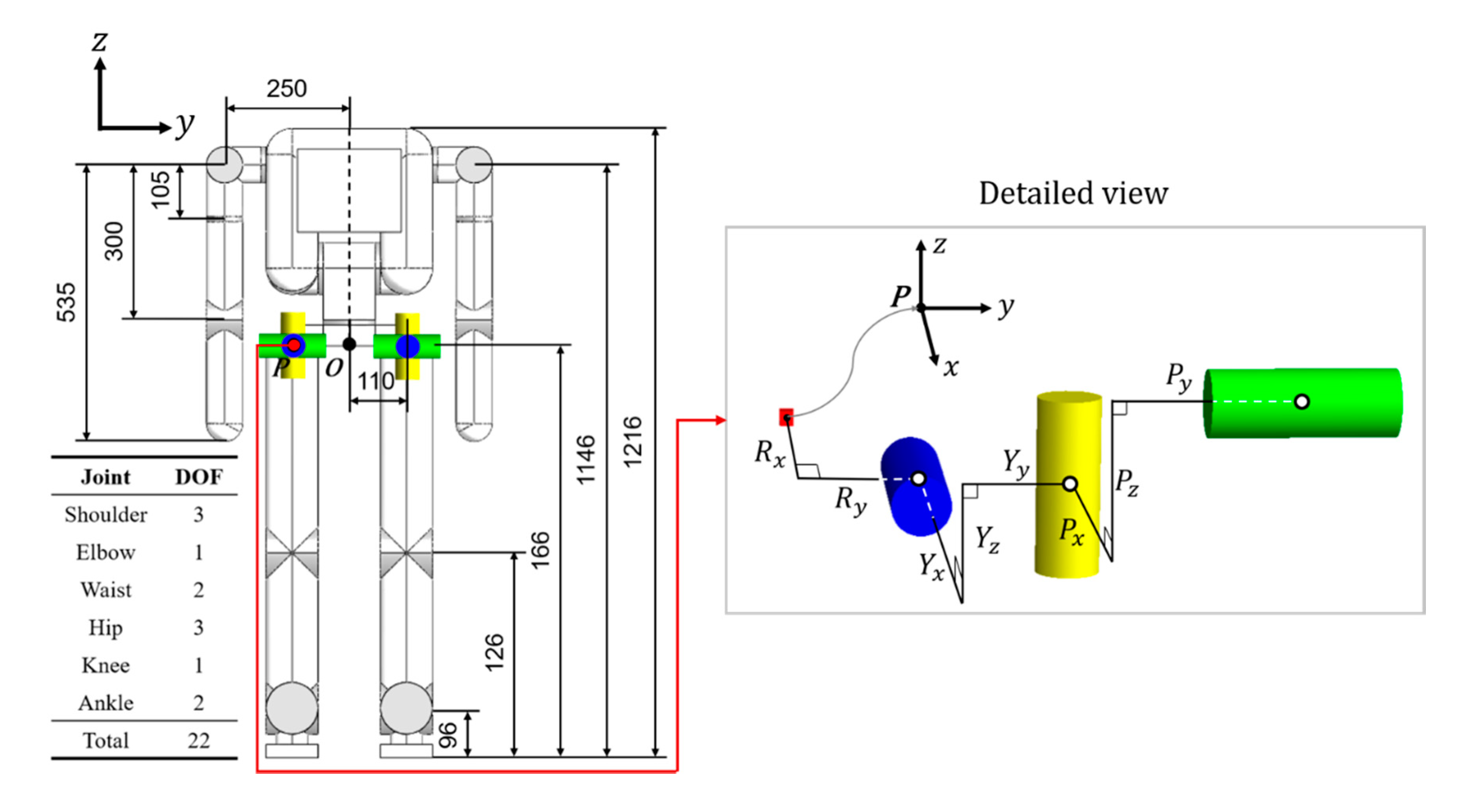
The humanoid robot used for simulation was designed to have a similar size to a young man. We selected the length and mass of each segment and the size of the humanoid robot by referring to the average body size of Koreans aged 16 to 19 [9]. Other kinematic parameters for the detailed design of the humanoid robot were based on the MAHRU humanoid robot, previously developed in our institute [10]. The robot had 22 degrees of freedom, weighed 57 kg, and had a height of 1.216 m and shoulder width of 0.5 m. The humanoid robot structure is detailed in Figure 1. Its thigh length and weight were 0.4 m and 5.5 kg, respectively, whereas its calf length and weight were 0.3 m and 3.5 kg, respectively, and its ankle length and weight were 0.07 m and 0.25 kg, respectively. Each foot was 0.026 m in height, 0.25 m in length, 0.1 m in width, and 0.75 kg in weight.
Although the original width between the left and right foot was 0.22 m, we varied it in each test model, depending on the selected offset in the hip joint along the Y axis. For example, a test model with a 0.03 m offset was designed with a width of 0.28 m between the feet.
3.2. Control Factors: Joint Offsets
We set the offsets among the three joints (roll, yaw, and pitch) in the humanoid robot hip as control factors. The hip joint used for simulation was composed in the sequence of roll, yaw, and pitch joints. The offset between the torso and roll joints along the X and Y axes was selected as a parameter because this joint did not have a preceding offset. The offset between the torso and roll joints along the Z axis was fixed and disregarded as a parameter because it changed the humanoid leg length.
For the roll–yaw joint and yaw–pitch joint, all offsets along the X, Y, and Z axes were selected. The offsets along the Z axis were negative because it was challenging to place a following joint higher than the preceding joint in practical mechanisms. The offsets at the joints that serve as parameters are detailed in Figure 1 (right graph), with each offset being denoted by the letter of the following joint and offset direction. For example, the offset between the torso and roll joints along the Y axis is denoted by Ry, and the offset between the yaw and pitch joints along the Z axis is denoted by Pz.
3.3. Noise Factors: Humanoid Motions
We set turning, forward, backward, and sideways walking motions as noise factors. As forward and backward are the most basic humanoid robot motions, they were selected as target motions. Moreover, turning and sideways walking were selected, given their distinctiveness compared with forward and backward motions, despite their lower occurrence frequencies. The walking patterns were generated by using the zero-moment point (ZMP) controller designed for the MAHRU humanoid robot [10].
For fair comparison during the optimization process, we set the movement pattern of each model’s feet to be the same. We fixed the following parameters related to feet motion generation as constant values:
- Step length: 200 mm for forward and backward walking and 100 mm for sideways walking;
- Maximum foot clearance (maximum lifting height of the feet during gait): 80 mm;
- Single and double support time for a stride: 800 ms and 200 ms;
The amplitude of the center-of-mass for generating the ZMP trajectory was set as a constant value of 650 mm.
3.3.1. Forward and Backward Walking
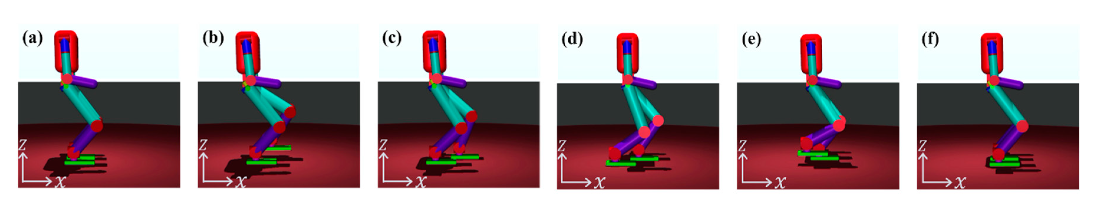
Forward and backward walking were set identically in the experiments because they occurred along the same axis. The humanoid only moved backward and forward while these motions were executed. During walking, the left foot moved first, and each foot completed three steps in the forward or backward direction. Hence, the humanoid robot moved 1 m in either direction, as shown in Figure 2.
3.3.2. Sideways Walking
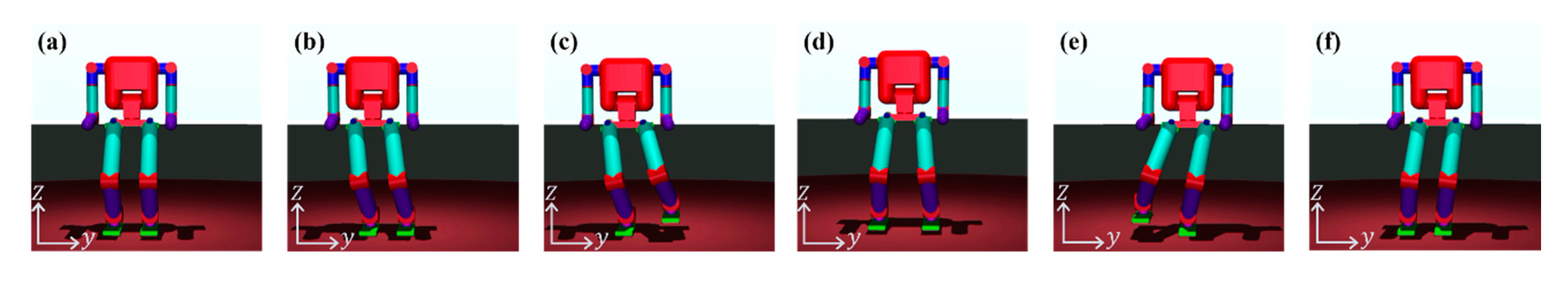
Sideways walking is a perpendicular motion, with respect to forward and backward walking, without rotating the humanoid robot body. Starting with the left foot, each one completed three steps. Thus, the humanoid robot moved 300 mm to the left after sideways walking, which proceeded as shown in Figure 3.
3.3.3. Turning
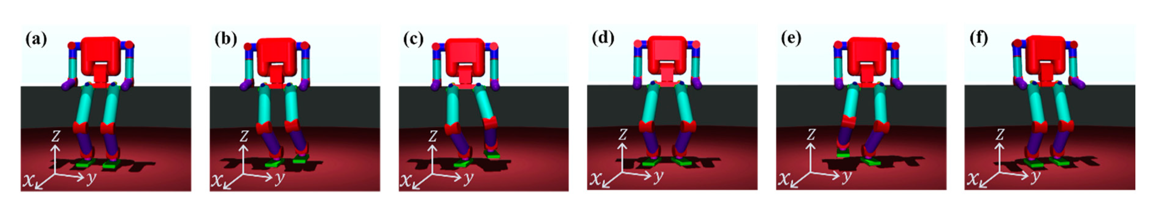
Unlike the previous motions, turning changes only the orientation of the body at a fixed position. The turning angle was set to 20° for the first experimental set and 15° for the second one, being smaller because the corresponding test model for the second stage had a smaller supporting polygon, leading to instability at larger angles. The supporting polygon is further explained in the corresponding discussion in Section 6. Starting with the left foot, the humanoid turned three times per trial, reaching overall turning angles of 60° and 45° for the first and second experimental sets, respectively. Figure 4 illustrates the turning motion.
4. Hip Joint Offset Optimization
4.1. First Experimental Set
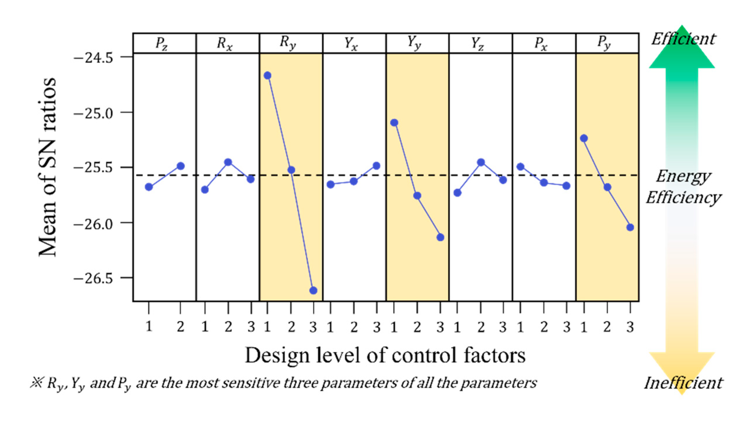
The first experimental set consisted of 18 trials, according to the L18 (21 × 37) orthogonal array. Table 1 and Table 2 list the parameter levels and results per trial according to these levels, respectively. As shown in Table 2, the SNR of the first test model was the highest at –23.923 when all control factor levels were 1. In contrast, the SNR of the third test model was the lowest. A higher SNR indicates that the objective function reached closer to the optimal value. Figure 5 shows the SNR of each factor according to its level. The highest SNR was achieved at the level of Pz = 2, Rx = 2, Ry = 1, Yx = 3, Yy = 1, Yz = 2, Px = 1, and Py = 1, and the factors with high sensitivities were Ry, Yy, and Py, with respective SNR variations of 1.90, 1.05, and 0.74. Factors with SNR variations below 0.3 were considered as insensitive.
4.2. Second Experimental Set
As the optimal points do not appear in the SNR graph of Figure 5, we considered only the three highly sensitive factors (Ry, Yy, and Py) for the second experimental set. The kinematics of the humanoid model for the second experimental set were designed using the optimal result from the first experimental set. Specifically, the value of each factor, including insensitive ones, was set to that retrieving the highest SNR in the first experimental set.
The second experimental set consisted of nine trials, according to the L9 (33) orthogonal array, with three factors. Table 3 and Table 4 list the parameter levels and results per trial according to these levels, respectively. The SNR was calculated as in the first experiment, obtaining the highest SNR at the ninth trial of –22.614 for the level of Ry = 3, Yy = 3, and Py = 2.
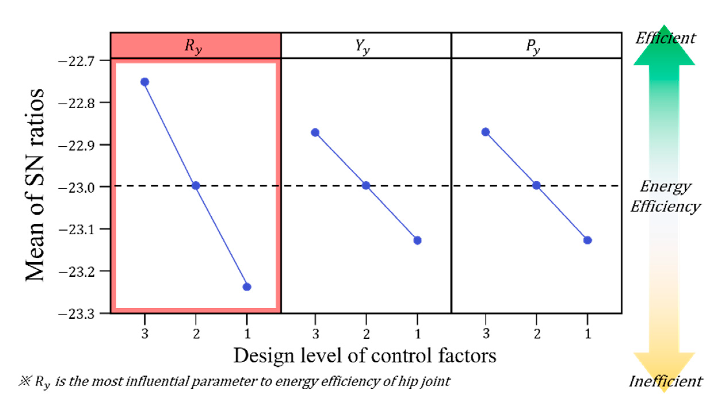
The SNRs, according to the level of each control factor in the second experimental set, are shown in Figure 6. The highest SNR was obtained when the three factors were at level 3, with Ry being the most sensitive factor with an SNR variation of 0.49 across all levels. The SNR variation for both Yy and Py was 0.25, with their sensitivities being lower than that of Ry. Although the results did not reach the optimal solution, we ended the optimization because of the limited range of feasible joint offsets.
5. Validation of Optimal Hip Joint Offsets
The near-optimal offsets of hip joints that minimize power consumption were obtained from the two experimental sets. Using the optimized model, we verified that power consumption was indeed reduced for various humanoid robot motions. The optimal values of the parameters are listed in Table 5, and Figure 7 shows the joint configuration and structure of the model after optimization in the second experimental set.
5.1. Forward and Backward Walking
Table 6 lists the power consumption in the hip, using the original model and the optimized models after the first and second experiments for forward and backward walking. For forward walking, the RMS power at the hip joint reduced by 18.07% and 26.92% for the models after the first and second optimizations, respectively, compared with the original model. For backward walking, the corresponding reductions were 17.26% and 25.68%.
5.2. Sideways Walking
Table 6 lists the power consumption in the hip joint for sideways walking. Compared to the original model, consumption decreased by 29.78% and 37.76% for the models after the first and second optimization, respectively. Like for forward and backward walking, power consumption gradually reduced from the original model to the models after the first and second optimizations.
5.3. Turning
The power consumption for turning using the original and optimized models is listed in Table 6. Note that the rotation angle for turning in the humanoid models was set to 15° equally. Like in the previous motions, consumption reduced in the hip joint, in this case by 21.81% and 30.09% for the models after the first and second optimization, respectively.
6. Discussion
We investigated the optimization for reducing power consumption at the hip of a humanoid robot via the Taguchi method. The two-stage optimization achieved a larger reduction in consumption than that obtained using only one stage. Power consumption at the hip was mainly influenced by the Y axis offset. Therefore, the closer the sides of the hip joint, the lower the energy consumption. The sum of RMS power consumption from the right hip joint (Powrms) over time during the motions is shown in Figure A1 and supplementary materials.
Humanoid robots implement zero-moment point walking to keep the point position inside the supporting polygon and thus stabilize the robot’s walking. The supporting polygon is a convex hull containing the contact points between the feet and ground. If both feet are close due to the hip joints being close, the supporting polygon becomes narrower. During single-leg support, the robot sways its upper body from side to side to place the zero-moment point inside the supporting polygon. Consequently, placing the hip joints closer reduces the area to move the zero-moment point to keep it within the supporting polygon while switching from double- to single-leg support. Then, the moment acting on the roll joint is decreased by the smaller moment arm of the upper body, related to the roll joint. Therefore, joint offsets along the Y axis are advantageous to improving energy efficiency by reducing power consumption in the roll joint, as both hip joints are close.
We explored the reason for the reduction of power consumption through bio-inspired analysis from human gait mechanics. The finding in this study is similar to the influence of the body’s center of gravity (COG) pathway on human walking efficiency. Minimizing the body’s COG, displaced from a level line of progression, is considered to be a major mechanism for reducing the muscular effort of walking and, consequently, for saving energy. The least energy would be used if the weight being carried remained at a constant height and followed a single central path. No additional lifting effort would then be needed to recover from the intermittent falls downward or laterally [11].
As an additional analysis, we compared the maximum required torque at the joint after optimization. The reduction of actuating torque is an important issue for reducing the weight of the actuators. Except for the pitch joint during the turning motion, all maximum torques generated at each joint were reduced by a minimum of 0.95% and a maximum of 44.67%. Before the optimization, the maximum torque of all joints was generated at a value of 70.91 Nm at the roll joint during the sideways walking motion. Through the optimization, this value was reduced to 59.15 Nm, which was also the maximum torque for the optimized model.
Although we obtained valuable insights on offset design, some limitations of this study remain to be addressed. We considered only mechanical power to represent power consumption, because it is impossible to calculate the electrical power dissipated in the actuator before selecting the motor and other electronic components. In addition, although the negative mechanical power can be restored using a regeneration system, we neglected this aspect because humanoid robots typically do not implement a regeneration system.
We expect to use the findings in this study to design an improved humanoid robot. By improving energy efficiency, the operating time of humanoid robots can be extended. As for future work, we plan to verify energy efficiency optimization while a humanoid robot performs various tasks. Moreover, we intend to extend joint offset optimization to include knee and ankle joints.
Supplementary Materials
The following are available online at https://www.mdpi.com/2076-3417/10/20/7287/s1. Video S1: The sum of RMS power consumption from the right hip joint of the original, first, and second optimized humanoid robot at the hip joint during the target motions.
Author Contributions
Conceptualization, J.K., J.Y., S.T.Y., Y.O., and G.L.; methodology, J.K., J.Y., and G.L; software, J.K., J.Y., Y.O., and G.L.; validation, J.K., J.Y., and G.L.; data analysis, J.K., J.Y., and G.L.; writing—original draft preparation, J.K. and G.L.; writing—review and editing, J.K., J.Y., Y.O., and G.L.; visualization, J.K. and G.L.; supervision, Y.O. and G.L.; project administration, Y.O. and G.L.; funding acquisition, Y.O. and G.L. All authors have read and agreed to the published version of the manuscript.
Funding
This research was funded by the Korea Institute of Science and Technology, KIST, Institutional Program (Project No. 2E29460-19-018) and the Chung-Ang University Research Scholarship Grants in 2020.
Acknowledgments
The authors thank Seung Jae Yoo from the Korea Institute of Science and Technology for his contributions to this work.
Conflicts of Interest
The authors declare no conflict of interest.
Appendix A
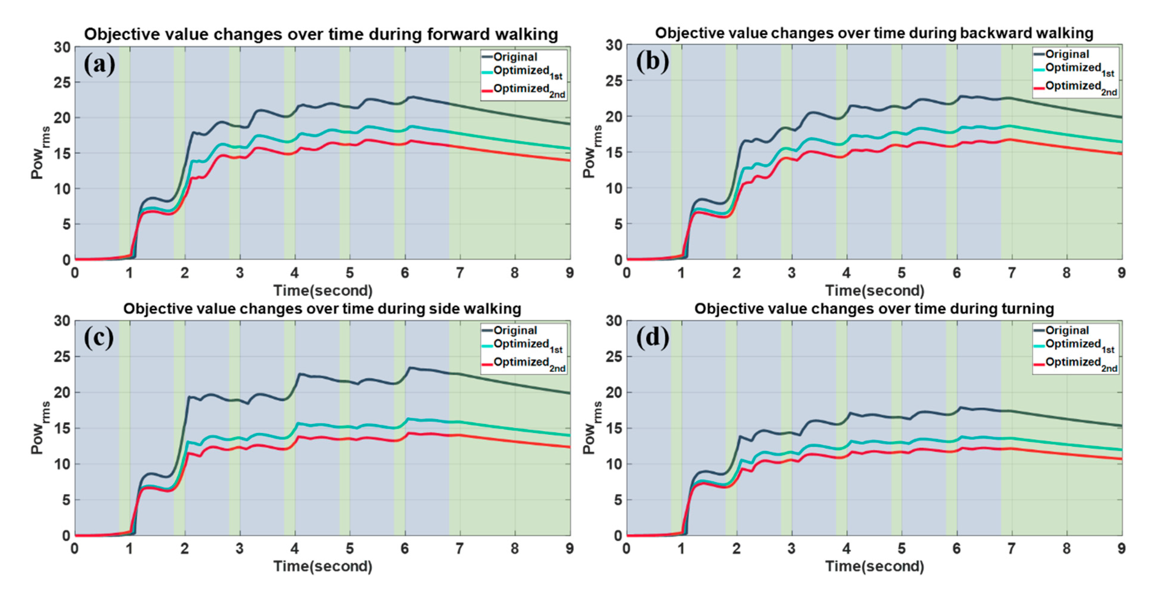
Figure A1 shows the sum of RMS power consumption from the right hip joint (Powrms) over time of the original, first, and second humanoid robot at the hip joint during the target motions.
Figure A1.
Objective value changes over time during (a) forward walking, (b) backward walking, (c) sideways walking, and (d) turning. Optimized 1st and 2nd indicate the models after the first and second optimization, respectively. Blue and green colored backgrounds indicate a single and double support phase during target motion, respectively.

References
- Zorjan, M.; Hugel, V.; Blazevic, P.; Borovac, B. Influence of rotation of humanoid hip joint axes on joint power during locomotion. Adv. Robot. 2015, 29, 707–719. [Google Scholar] [CrossRef]
- Lee, J.; Lee, G.; Oh, Y. Energy-efficient robotic leg design using redundantly actuated parallel mechanism. In Proceedings of the IEEE International Conference on Advanced Intelligent Mechatronics (AIM), Munich, Germany, 3–7 July 2017. [Google Scholar]
- Negrello, F.; Garabini, M.; Catalano, M.G.; Kryczka, P.; Choi, W.; Caldwell, D.G.; Bicchi, A.; Tsagarakis, N.G. Walk-man humanoid lower body design optimization for enhanced physical performance. In Proceedings of the IEEE International Conference on Robotics and Automation (ICRA), Stockholm, Sweden, 16–21 May 2016. [Google Scholar]
- Tsagarakis, N.G.; Morfey, S.; Dallali, H.; Medrano-Cerda, G.A.; Caldwell, D.G. An asymmetric compliant antagonistic joint design for high performance mobility. In Proceedings of the IEEE/RSJ International Conference on Intelligent Robots and Systems (IROS), Tokyo, Japan, 3–7 November 2013. [Google Scholar]
- Tsui, K.L. An overview of Taguchi method and newly developed statistical methods for robust design. IIE Trans. 1992, 24, 44–57. [Google Scholar] [CrossRef]
- Hong, H.S.; Seo, T.; Kim, D.; Kim, S.; Kim, J. Optimal design of hand-carrying rocker-bogie mechanism for stair climbing. J. Mech. Sci. Technol. 2013, 27, 125–132. [Google Scholar] [CrossRef]
- Sung, T.; Oh, D.; Jin, S.; Seo, T.W.; Kim, J. Optimal design of a micro evaporator with lateral gaps. Appl. Therm. Eng. 2009, 29, 2921–2926. [Google Scholar] [CrossRef]
- Jugulum, R.; Taguchi, S. Computer-Based Robust Engineering: Essentials for DFSS, 1st ed.; ASQ Quality Press: Milwaukee, WI, USA, 2004; p. 95. [Google Scholar]
- Size Korea. Available online: https://sizekorea.kr/page/report/1 (accessed on 4 January 2020).
- Kwon, W.; Kim, H.K.; Park, J.K.; Roh, C.H.; Lee, J.; Park, J.; Kim, W.K.; Roh, K. Biped humanoid robot Mahru III. In Proceedings of the IEEE-RAS International Conference on Humanoid Robots, Pittsburgh, PA, USA, 29 November–1 December 2007. [Google Scholar]
- Perry, J.; Burnfield, J.M. Center of Gravity Alignment Modulation. In Gait Analysis: Normal and Pathological Function, 2nd ed.; SLACK Incorporated: Thorofare, NJ, USA, 2010; pp. 40–43. [Google Scholar]
Figure 1.
Humanoid robot simulation model (units in millimeters) for optimization. The parameters in the detailed view correspond to joint offsets. The design parameters were configured based on the front view of the hip joint for the right leg. The roll, yaw, and pitch joints are represented as blue, yellow, and green colors, respectively.

Figure 2.
Forward walking. (a) Initial position, (b) left foot lifting, (c) left foot lowering after swing, (d) center-of-mass forward displacement, (e) right foot lifting, and (f) motion completion.
Figure 2.
Forward walking. (a) Initial position, (b) left foot lifting, (c) left foot lowering after swing, (d) center-of-mass forward displacement, (e) right foot lifting, and (f) motion completion.

Figure 3.
Sideways walking. (a) Initial position, (b) moving zero-moment point above the right foot, (c) left foot lifting, (d) left foot lowering after swing, (e) moving zero-moment point above the left foot and right foot lifting, (f) right foot lowering and motion completion.
Figure 3.
Sideways walking. (a) Initial position, (b) moving zero-moment point above the right foot, (c) left foot lifting, (d) left foot lowering after swing, (e) moving zero-moment point above the left foot and right foot lifting, (f) right foot lowering and motion completion.

Figure 4.
Turning. (a) Initial position, (b) moving zero-moment point above the right foot, (c) left-foot lifting and both left leg and body turning, (d) left foot lowering, (e) right foot lifting and both right leg and body turning, and (f) motion completion.
Figure 4.
Turning. (a) Initial position, (b) moving zero-moment point above the right foot, (c) left-foot lifting and both left leg and body turning, (d) left foot lowering, (e) right foot lifting and both right leg and body turning, and (f) motion completion.

Figure 5.
Signal-to-noise ratios (SNRs) of the eight parameters during the first experiment. The three most influential factors are highlighted in yellow.
Figure 5.
Signal-to-noise ratios (SNRs) of the eight parameters during the first experiment. The three most influential factors are highlighted in yellow.

Figure 6.
SNRs of three sensitive parameters during the second experiment. The most influential factor is Ry, highlighted in red.
Figure 6.
SNRs of three sensitive parameters during the second experiment. The most influential factor is Ry, highlighted in red.

Figure 7.
Hip joint configuration of (a) the original model and (b) the model after the second optimization.
Figure 7.
Hip joint configuration of (a) the original model and (b) the model after the second optimization.


Table 1.
Levels of control factors for the first experimental set.
| Level | Control Factor (mm) | |||||||
|---|---|---|---|---|---|---|---|---|
| Pz | Rx | Ry | Yx | Yy | Yz | Px | Py | |
| 1 | −10 | −10 | −10 | −10 | −10 | −20 | −10 | −10 |
| 2 | 0 | 0 | 0 | 0 | 0 | –10 | 0 | 0 |
| 3 | - | 10 | 10 | 10 | 10 | 0 | 10 | 10 |
Table 2.
Design, results, and SNRs of first experimental set. (The highest SNR is boldfaced.)
| Test | Control Factor | Noise Factor | SNR | ||||||||||
|---|---|---|---|---|---|---|---|---|---|---|---|---|---|
| Pz | Rx | Ry | Yx | Yy | Yz | Px | Py | Forward Walking | Backward Walking | Sideways Walking | Turning | ||
| Objective Function (W) | |||||||||||||
| 1 | 1 | 1 | 1 | 1 | 1 | 1 | 1 | 1 | 17.237 | 19.384 | 13.928 | 10.970 | −23.923 |
| 2 | 1 | 1 | 2 | 2 | 2 | 2 | 2 | 2 | 21.852 | 21.427 | 19.928 | 14.353 | −25.854 |
| 3 | 1 | 1 | 3 | 3 | 3 | 3 | 3 | 3 | 24.439 | 25.420 | 26.282 | 17.854 | −27.507 |
| 4 | 1 | 2 | 1 | 1 | 2 | 2 | 3 | 3 | 19.349 | 20.095 | 18.557 | 13.403 | −25.126 |
| 5 | 1 | 2 | 2 | 2 | 3 | 3 | 1 | 1 | 20.484 | 21.175 | 19.856 | 13.993 | −25.617 |
| 6 | 1 | 2 | 3 | 3 | 1 | 1 | 2 | 2 | 21.263 | 22.027 | 21.309 | 14.951 | −26.061 |
| 7 | 1 | 3 | 1 | 2 | 1 | 3 | 2 | 3 | 18.467 | 19.167 | 17.206 | 12.542 | −24.631 |
| 8 | 1 | 3 | 2 | 3 | 2 | 1 | 3 | 1 | 21.706 | 20.175 | 18.439 | 13.416 | −25.435 |
| 9 | 1 | 3 | 3 | 1 | 3 | 2 | 1 | 2 | 23.512 | 24.215 | 24.664 | 16.653 | −27.043 |
| 10 | 2 | 1 | 1 | 3 | 3 | 2 | 2 | 1 | 18.416 | 19.150 | 16.947 | 12.493 | −24.583 |
| 11 | 2 | 1 | 2 | 1 | 1 | 3 | 3 | 2 | 19.613 | 20.351 | 18.673 | 13.459 | −25.214 |
| 12 | 2 | 1 | 3 | 2 | 2 | 1 | 1 | 3 | 23.605 | 24.906 | 24.626 | 16.663 | −27.121 |
| 13 | 2 | 2 | 1 | 2 | 3 | 1 | 3 | 2 | 19.379 | 20.073 | 18.582 | 13.406 | −25.130 |
| 14 | 2 | 2 | 2 | 3 | 1 | 2 | 1 | 3 | 18.022 | 19.990 | 18.280 | 11.949 | −24.776 |
| 15 | 2 | 2 | 3 | 1 | 2 | 3 | 2 | 1 | 21.555 | 22.367 | 21.442 | 15.045 | −26.157 |
| 16 | 2 | 3 | 1 | 3 | 2 | 3 | 1 | 2 | 18.453 | 19.177 | 17.186 | 12.513 | −24.625 |
| 17 | 2 | 3 | 2 | 1 | 3 | 1 | 2 | 3 | 22.146 | 23.095 | 22.925 | 15.855 | −26.534 |
| 18 | 2 | 3 | 3 | 2 | 1 | 2 | 3 | 1 | 20.096 | 21.019 | 19.397 | 14.175 | −25.511 |
Table 3.
Levels of control factors for the second experimental set.
| Level. | Control Factor (mm) | ||
|---|---|---|---|
| Ry | Yy | Py | |
| 1 | 0 | 0 | 0 |
| 2 | −2.5 | −2.5 | −2.5 |
| 3 | −5 | −5 | −5 |
Table 4.
Design, results, and SNRs of the second experimental set. (The highest SNR is boldfaced.)
| Test | Control Factor | Noise Factors | SNR | |||||
|---|---|---|---|---|---|---|---|---|
| Ry | Yy | Py | Forward Walking | Backward Walking | Sideways Walking | Turning | ||
| Objective function (W) | ||||||||
| 1 | 1 | 1 | 1 | 16.591 | 17.387 | 13.951 | 10.832 | −23.471 |
| 2 | 1 | 2 | 2 | 16.212 | 16.953 | 13.572 | 10.518 | −23.248 |
| 3 | 1 | 3 | 3 | 15.721 | 16.520 | 13.111 | 10.198 | −22.988 |
| 4 | 2 | 1 | 2 | 16.016 | 16.747 | 13.347 | 10.352 | −23.130 |
| 5 | 2 | 2 | 3 | 15.528 | 16.322 | 12.875 | 10.040 | −22.867 |
| 6 | 2 | 3 | 1 | 15.764 | 16.532 | 13.120 | 10.218 | −23.001 |
| 7 | 3 | 1 | 3 | 15.349 | 16.122 | 12.660 | 9.881 | −22.750 |
| 8 | 3 | 2 | 1 | 15.573 | 16.337 | 12.901 | 10.034 | −22.881 |
| 9 | 3 | 3 | 2 | 15.113 | 15.871 | 12.491 | 9.690 | −22.614 |
Table 5.
Parameter values of the model after the second optimization.
| Parameter | Pz | Rx | Ry | Yx | Yy | Yz | Px | Py |
|---|---|---|---|---|---|---|---|---|
| Value (mm) | 0 | 0 | −15 | 10 | −15 | 0 | −10 | −15 |
Table 6.
Root-mean-square (RMS) power reduction using an optimized model in humanoid hip joints during target motions.
Table 6.
Root-mean-square (RMS) power reduction using an optimized model in humanoid hip joints during target motions.
| Model | Forward Walking | Backward Walking | Sideways Walking | Turning | ||||
|---|---|---|---|---|---|---|---|---|
| Powrms (W) | Reduction (%) | Powrms (W) | Reduction (%) | Powrms (W) | Reduction (%) | Powrms (W) | Reduction (%) | |
| Original | 20.250 | – | 21.013 | – | 19.868 | – | 15.325 | – |
| First Optimization | 16.591 | 18.07 | 17.387 | 17.26 | 13.951 | 29.78 | 11.983 | 21.81 |
| Second Optimization | 14.799 | 26.92 | 15.617 | 25.68 | 12.365 | 37.76 | 10.713 | 30.09 |
Publisher’s Note: MDPI stays neutral with regard to jurisdictional claims in published maps and institutional affiliations. |
© 2020 by the authors. Licensee MDPI, Basel, Switzerland. This article is an open access article distributed under the terms and conditions of the Creative Commons Attribution (CC BY) license (http://creativecommons.org/licenses/by/4.0/).
Share and Cite
MDPI and ACS Style
Kim, J.; Yang, J.; Yang, S.T.; Oh, Y.; Lee, G. Energy-Efficient Hip Joint Offsets in Humanoid Robot via Taguchi Method and Bio-inspired Analysis. Appl. Sci. 2020, 10, 7287. https://doi.org/10.3390/app10207287
AMA Style
Kim J, Yang J, Yang ST, Oh Y, Lee G. Energy-Efficient Hip Joint Offsets in Humanoid Robot via Taguchi Method and Bio-inspired Analysis. Applied Sciences. 2020; 10(20):7287. https://doi.org/10.3390/app10207287
Chicago/Turabian StyleKim, Jihun, Jaeha Yang, Seung Tae Yang, Yonghwan Oh, and Giuk Lee. 2020. "Energy-Efficient Hip Joint Offsets in Humanoid Robot via Taguchi Method and Bio-inspired Analysis" Applied Sciences 10, no. 20: 7287. https://doi.org/10.3390/app10207287
Note that from the first issue of 2016, this journal uses article numbers instead of page numbers. See further details here.