T-Spline Surface Toolpath Generation Using Watershed-Based Feature Recognition

1
School of Mechanical Engineering and Automation, Beihang University, Beijing 100191, China
2
MIIT Key Laboratory of Aeronautics Intelligent Manufacturing, Beihang University, Beijing 100191, China
*
Author to whom correspondence should be addressed.
Appl. Sci. 2020, 10(19), 6790; https://doi.org/10.3390/app10196790
Submission received: 3 August 2020
/
Revised: 24 September 2020
/
Accepted: 25 September 2020
/
Published: 28 September 2020
(This article belongs to the Section Mechanical Engineering)
Abstract
:Featured Application
The proposed method can be used for manufacturing of a freeform surface with convex or concave features. Due to the advantages of T-spline and watershed technology, the proposed method can divide a surface into a set of sub-regions with boundaries defined mathematically, and the optimized multi-rectangles toolpath generation has advantages for toolpath length and toolpath reversing number.
Abstract
The freeform surface is treated as a single machining region for most traditional toolpath generation algorithms. However, due to the complexity of a freeform surface, it is impossible to produce a high-quality surface using one unique machining process. Hence, region-based methods are widely investigated for freeform surface machining to achieve an optimized toolpath. The Non-Uniform Rational B-spline Surface (NURBS) represented freeform surface is not suitable for region-based toolpath generation because of the surface gaps caused by NURBS trimming and merging operations. To solve the limitation of the NURBS, T-spline is proposed with the advantages of being gap-free, having less control points, and local refinement, which is an ideal tool for region-based toolpath generation. Thus, T-spline is introduced to represent a freeform surface for its toolpath generation in the paper. A region-based toolpath generation method for the T-spline surface is proposed based on watershed technology. Firstly, watershed-based feature recognition is presented to divide the T-spline surface into a set of sub-regions. Secondly, the concept of a PolyBoundingBox that consists of a set of minimum bounding boxes is proposed to describe the sub-regions, and Manufacturing-Suitable Regions are constructed with the help of T-spline local refinement and the PolyBoundingBox. In the end, an optimized multi-rectangles toolpath generation algorithm is applied for sub-regions. The proposed method is tested using three synthetic T-spline surfaces, and the comparison results show the advantage in toolpath length and toolpath reversing number.
1. Introduction
Freeform surfaces play a critical role in the field of shipbuilding, automotive, and aerospace. Toolpath generation is the fundamental task for freeform surface manufacturing. The ideal toolpath should be generated uniformly across the whole surface, and the scallop height should be maintained below the specified value. From the geometric point of view, the freeform surface is generally designed feature-by-feature to satisfy the modeling functionality, and different features usually have diverse manufacturing properties. Therefore, it is difficult to achieve a consistent scallop using single toolpath generation algorithms for different features, such as the iso-parametric algorithm [1], iso-planner algorithm [2], and iso-scallop algorithm [3]. Hence, a region-based toolpath generation algorithm has been investigated in the last two decades to solve the problem [4].
NURBS (Non-Uniform Rational B-spline Surface) is adopted mostly for region-based toolpath generation algorithms, and the boundaries of the sub-regions are represented using analytical curves or discrete points. Hence, a freeform surface behaves like trimmed NURBS after segmentation, which will introduce gaps near the boundaries of sub-regions, and a lot of time-consuming work is needed for toolpath repair with human–machine interaction. T-spline is the latest technology for shape modeling of a freeform surface, and can represent multiple patches watertightly without introducing gaps, which is an ideal tool for region-based freeform surface toolpath generation. Hence, T-spline is adopted to represent a freeform surface for region-based toolpath generation. In our previous research work, region-based toolpath generation algorithms for T-spline surfaces are proposed [5,6,7] without considering T-spline surface features. However, this feature is important not only for modeling, but also for manufacturing. Hence, feature recognition technology is studied for region-based toolpath generation in this study.
It is imperative to recognize the machining features of the T-spline surface for toolpath generation, specifically to segment the T-spline surface into different sub-regions with feature-preserving in order to achieve the high-quality machining toolpath of T-spline surface. In our previous research work [7], the concept of Manufacturing-Suitable Region (MSR) was proposed that consists of sub-regions of a T-spline surface, and owns similar machining properties. The concept of MSR provides new possibilities for region-based T-spline toolpath generation, and three technical routes were presented for the MSRs construction of the T-spline surface (manual, human–machine interaction, and automatic). In the report, the automatic segmentation method is investigated based on watershed technology, which has been applied successfully in image segmentation and mesh segmentation.
In the paper, watershed-based feature recognition technology is employed to divide the T-spline surface into a set of MSRs, and the toolpath for ball-end finishing milling is generated using the optimized multi-rectangle toolpath generation algorithm for each MSR. The paper is organized as follows. The basic concepts of T-spline and feature recognition technology are reviewed in Section 2. Section 3 presents the proposed method consists of watershed-based feature recognition, MSR generation using T-spline local refinement and PolyBoundingBox construction, and optimized multi-rectangle toolpath generation algorithm. Experiments and discussion are given in Section 4. We end with the conclusion in Section 5.
2. Related Work
2.1. T-Spline and MSR
T-spline is the latest geometric modeling technology for freeform surface that can address the important limitations of NURBS. T-spline is a superset of NURBS, so the advantages and algorithm based on NURBS can be extended to T-spline naturally. In addition to this, T-spline allows control points to terminate at partial row (or column), hence T-spline can model a complicated freeform surface as a single, gap-free geometry without introducing redundant control points. Beyond that, trimming and merging the NURBS can be represented by a single watertight T-spline surface due to the capability of truly local refinement.
As a result of the outstanding characteristics of the T-spline surface, T-spline provides the ability to divide a freeform surface into a set of gap-free sub-regions that can be described using the concept of Manufacturing-Suitable Region (MSR) proposed in our previous research work [7]. MSR is composed of a set of faces that is effective to describe the sub-regions of T-spline surface for manufacturing. MSR has the following significant features:
- Every MSR specifies a set of sub-regions that is convenient for toolpath generation in the region.
- Geometric and manufacturing properties are similar maximally inside each MSR, and minimally between each of MSRs.
- The continuity between each of MSRs is guaranteed by the properties of T-spline.
MSR consists of a set of faces that are the basic elements of T-spline surface. T-spline surface is defined based on a control grid called T-mesh, and defined mathematically using the following equation [8]:
where Pi = (xi, yi, zi, wi) are the control points in homogeneous coordinate system, and Bi(s,t) are the T-spline blending functions given by the following:
Ni(s) and Ni(t) are B-spline basis functions calculated iteratively as follows:
In our research, k is set to 3 in Equation (3) for calculation of the bi-cubic T-spline surface.
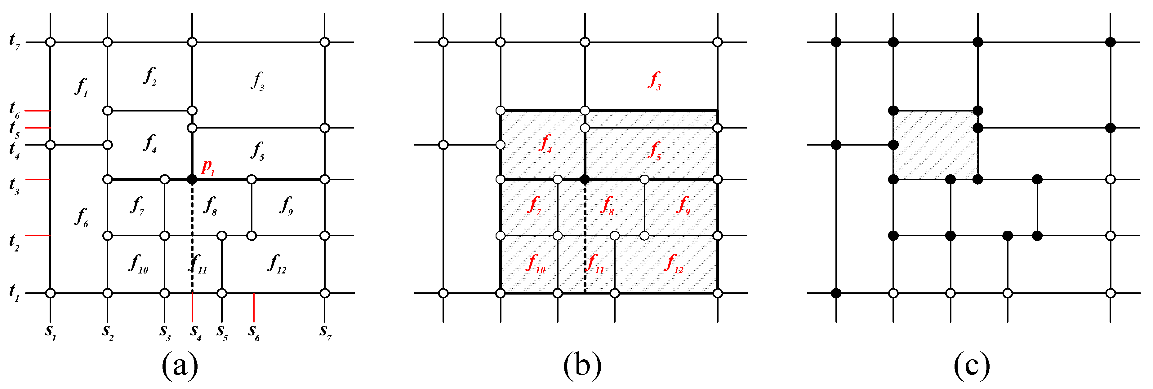
For each control point Pi of T-spline surface, its influence domain is constructed by its two knot vectors determined using ray intersection method [9]. An overlap operation can be executed between the influence domain of the control point and every face of T-spline surface. The influence point has contribution for face calculation when the overlap is existent. A set of influence points for each face are initialized after the overlap operation is accomplished for all control points, and T-spline surface can be evaluated face-by-face. Hence, toolpath can be generated for each MSR independently, which is beneficial for region-based toolpath generation.
Figure 1a presents knot vectors calculation for control point p1 in (s4,t3), five knot vectors are required for cubic T-spline in each parametric direction, and the knot vectors for p1 are [s2,s3,s4,s6,s7] and [t1,t2,t3,t5,t6]. Figure 1b shows the influence domain of control point p1 that is filled with shaded area, and the faces marked by red label have overlap with the influence domain of p1. Figure 1c gives the influence points marked by solid circle that have non negative contribution for the shaded face.
2.2. Feature Recognition
Feature recognition is a process of reinterpreting a design model for manufacturing activities automatically [10], and is widely investigated for the segmentation of B-rep model, mesh, and a freeform surface. A number of feature recognition algorithms have been designed in the past few years, and a critical review of feature recognition was presented [10]. Zhang et al. [11] presented a surface-based approach for geometric feature recognition for the purposed of automating the process planning of freeform surface machining. The freeform surface is represented by trimmed NURBS, and five geometric features are defined and classified according to the surface normal. Sheen and You [12] proposed an efficient method for identifying machining features of B-rep model, and different kinds of 3-axis toolpath can be automatically generated for various machining features. Sunil and Pande [13] proposed a novel approach for automatic feature recognition from freeform surface represented in STL format. The geometric properties of curvature and normal are employed to define the fundamental shapes of the surface, and two-stage segmentation (dense/coarse mesh segmentation) for the freeform surface is applied. Zhang et al. [14] presented an efficient method for feature extraction of the B-rep model based on Gauss and Mean curvature for moldability analysis. Wang et al. [15] described a method of machining feature recognition for a freeform surface based on critical points extracted by Morse theory and the relationship between machining patches. Gupta and Gurumoorthy [16] proposed an algorithm for extracting freeform surface features from the geometry and topology information of a surface automatically. Li et al. [17] defined a new type of manufacturing feature generally used in aircraft structural model called ribs, and feature recognition for the ribs feature was presented that can be easily used for CNC toolpath programming. Liu et al. [18] proposed a concept of multi-perspective dynamic feature, which can divide a freeform surface into a set of sub-features with dynamic information to support adaptive NC machining applications. Various methods or technologies have been proposed to demonstrate the capability and efficiency of feature recognition for freeform surface applications from the existent literature. In this paper, watershed technology is introduced for feature recognition of T-spline surface due to its robust and successful application for image and mesh segmentation [19,20,21,22,23,24,25].
Watershed technology has been first defined for image processing [19], and has been extended for mesh segmentation in the last two decades. Mangan and Whitaker [20] firstly extended watershed technology from image processing to mesh segmentation. The total curvature of the surface is employed in this method to divide the surface into regions that are bounded by higher curvature. The proposed method is sensitive to the user-specified threshold. Pulla et al. [21] improved the quality of mesh segmentation by increasing the accuracy of the curvature estimates by use of mean, root-mean-square, and absolute curvatures. The program is semi-automatic since the result is also dependent on the user input threshold. Page and Koschan [22] introduced the fast marching watersheds algorithm for mesh segmentation based on human vision theory known as the minima rule. Wu et al. [23] outlined an approach based on mesh connectivity relationships that apply to watershed algorithms to detect prong features. Romstad and Etzelmuller [24] described a new method for terrain surface segmentation using the mean-curvature watershed, which can produce two sets of terrain units, depressions, and hills. Comic et al. [25] presented a new approach for discrete Morse gradient construction on mesh surface endowed by a scalar function starting from watershed decomposition.
3. Proposed Method
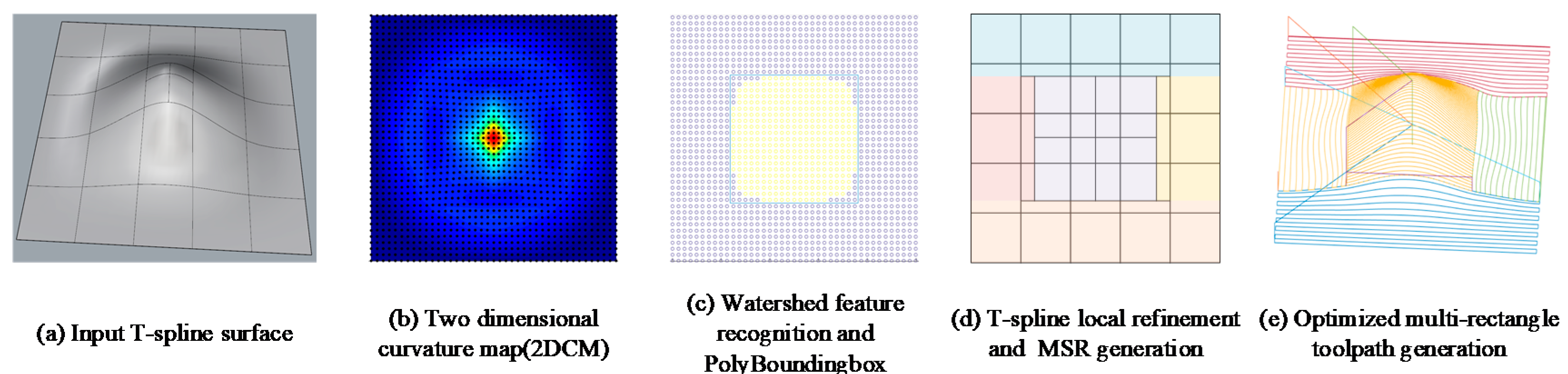
In this section, watershed-based feature recognition is adopted for toolpath generation of T-spline surface. Firstly, a discrete two-dimensional curvature map is constructed based on T-spline surface uniform sampling, and watershed technology is employed to extract the meaningful feature from the curvature map. Secondly, the extracted feature undergoes post-processing using T-spline local refinement and PolyBoundingBox for MSR generation, and the T-spline surface is divided into a set of sub-regions with boundaries defined mathematically. Thirdly, the toolpath is generated for MSRs using an optimized multi-rectangle algorithm [5] to improve efficiency regarding the tool reversing number. Figure 2 shows the proposed method in a flow chart.
3.1. Watershed-Based Feature Recognition
The watershed concept is one of the classic tools for image segmentation, which simulates water rising on the gray level or gradient magnitude of the input image from the local minima or maxima [26]. A continuous height function f should be defined over the entire image domain, then the ‘flooding’ starts from local minima of the image and incrementally fill the basins until it connects to its neighbours. Watershed extracted boundaries are formed where the water spills over between two neighbouring basins. The watershed technology was successfully extended to three-dimensional mesh segmentation by using the discrete curvature at each mesh vertex as height function [20]. In the paper, watershed technology is firstly introduced into the T-spline surface that can be described using two-dimensional parametric space. In the section, a two-dimensional curvature map is constructed for T-spline surface as height function. After that, T-spline surface can be divided into a set of sub-regions using watershed technology.
3.1.1. Two-Dimensional Curvature Map Construction
Curvatures are the fundamental attribute that expose the convexity and concavity of freeform surface, which describe the inherent properties of freeform surface and can be used to guide the distribution of surface feature. Typically, the principal curvatures at surface points denoted kmin and kmax are the minimum curvature and maximum curvature, and the Gaussian curvature kgaussian and mean curvature kmean can be deduced by kmin and kmax, and vice versa. In the study, root-mean-square curvature krmc is adopted for feature recognition that has been demonstrated in previous research work. The curvatures can be calculated by means of first and second fundamental forms of the T-spline surface.
For T-spline surface in Equation (1), the first fundamental form (I) is given by
where
The second fundamental form (II) is given by
where
and n is the surface unit normal given by
Hence, the gaussian curvature (kgaussian), mean curvature (kmean), and two principal curvatures (kmax, kmin) are calculated as follows respectively:
And the root-mean-square curvature (krmc) is defined as below:
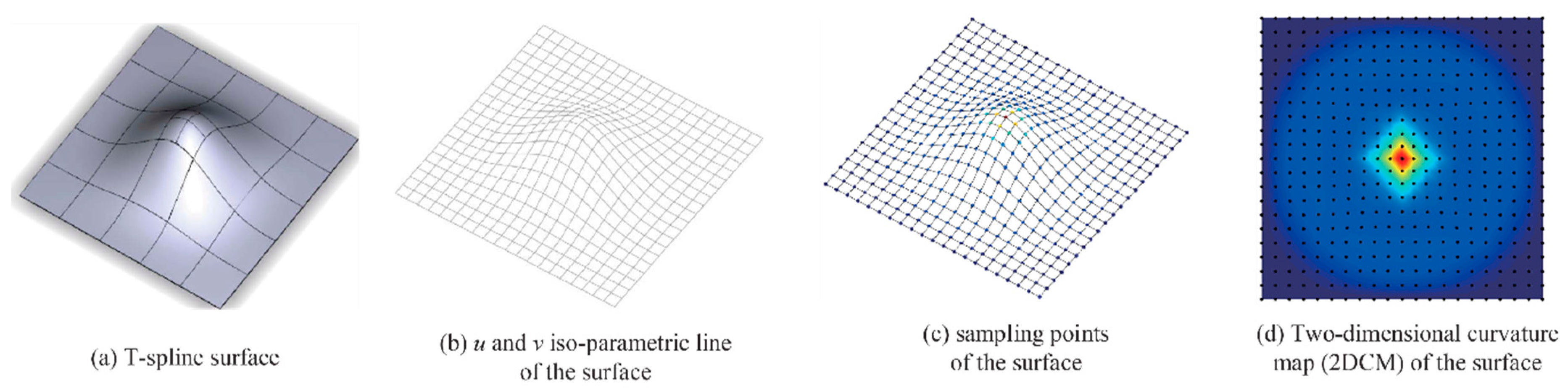
Curvatures are calculated for each point generated on T-spline surface using uniform sampling. Hence, a two-dimensional curvature map (2DCM) is defined in T-spline parametric space, where T-spline parameters (s,t) are employed as the (x,y) coordinates of the 2DCM, and the curvature information is employed as the z value of the 2DCM. The resolution of the 2DCM is decided by the points sampling frequency. High sampling frequency can generate a dense map that will improve the feature recognition accuracy with high computation cost and vice versa.
An example of T-spline surface 2DCM is given as shown in Figure 3: (a) presents the input T-spline surface, (b) gives the u and v iso-parametric lines of T-spline surface, (c) shows the sampling points colored by root mean square curvature, (d) projects the uniform sampling points on parametric space and colored in interpolation mode. It is evident that the concave and convex regions can be successfully delineated from the 2DCM intuitionally, and the feature recognition procedure will be presented in the next section.
3.1.2. Feature Recognition Using Watershed Technology
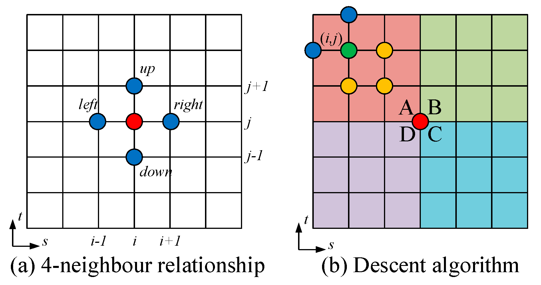
The point on 2DCM is denoted by xi that has a value of height function defined by root mean square curvature, and has a set of connected neighbouring points on 2DCM. Let X be the set of all points on 2DCM. For each xi ⊆ X, 4-neighbour of xi are employed for processing. We traverse each xi on 2DCM, the xi moves around its 4-neighbour depending on the connectivity and curvature descant. The topology of the 2DCM is described by rectilinear grid. Thus, the surface segmentation results affected by the height function is 2DCM. The procedure of watershed segmentation is shown as below:
- (1)
- Find the local maxima of 2DCM, and allocate labels for them as initial markers. Once the 2DCM is defined over T-spline surface, initial labels need to be specified for the whole surface. In order to figure out the problem of over-segmentation, a set of markers is positioned on 2DCM with unique labels. The markers can be used if the main parts of the surface are known, which can obtain the desired segmentation efficiently. Each initial marker has a one-to-one relationship to a specific watershed sub-region, thus the number of initial markers is equal to the final number of watershed sub-regions. The initial marker can be selected automatically or manually, and is generally difficult to obtain automatically without any user interaction. Selecting markers is a crucial and complicated task for watershed technology. For the sake of simplification, local maximum points are considered as markers in the paper.
- (2)
- Adopt descent algorithm for initial markers. The watershed region is extracted from each initial marker by using a root-mean-square curvature descent algorithm on the 2DCM. Each point on the 2DCM tested by the descent algorithm is labeled with the same specified label of the initial marker. The unlabeled points are searched along the 4-neighbour of each point on the 2DCM. As shown in Figure 4a, given a point indexed by (i,j) on the 2DCM, the position of 4-neighbour points can be obtained concisely: the up point is indexed by (i,j+1), down point indexed by (i,j-1), left point indexed by (i-1,j), right point indexed by (i+1,j). The descent algorithm is explained with the help of Figure 4b. For each initial marker (red point in Figure 4b), four areas are generated by 4-neighbour points and are handled using a similar method. Area A is taken as an example for more details. The green point is an arbitrary point pi,j in area A, three candidate points are chosen for test of pi,j that are marked in yellow, and the test is passed for pi,j when equation 11 is true.
3.2. MSR Generation Using T-Spline Local Refinement
After segmenting the T-spline surface into a set of sub-regions using watershed technology, the boundary of each sub-region can be described by means of sampling points, which is inaccurate to describe the boundaries of sub-regions and is troublesome for toolpath generation of sub-regions. The concept of Manufacturing-Suitable Region (MSR) is introduced to construct the boundary for sub-regions, which has been demonstrated for region-based T-spline toolpath generation in our previous work [7]. The MSR is a regular region that is composed of a set of T-spline faces. Toolpath continuity near boundaries of MSR-based sub-regions is guaranteed by the properties of T-spline. The MSR is constructed using T-spline local refinement based on segmented 2DCM, which can insert control points locally without changing the surface. MSR generation is an expanding method starting from one sub-region to another one, convex and concave sub-regions are commonly considerable for freeform surface toolpath generation. Hence, the construction of MSRs extends from convex or concave sub-regions to flat sub-regions in the paper. MSR generation generally includes two stages to execute T-spline local refinement, the topological stage and the geometrical stage.
3.2.1. Topological Stage of MSR Generation
The topological stage of MSR serves the purpose of new control points insertion near the boundaries of sub-regions. In this section, the concept of PolyBoundingBox is proposed to insert control points based on the minimum bounding box of sub-regions. The minimum bounding box for the sub-region is the box with the smallest Euclidean distance measurement for all sampling points in the sub-region. The minimum bounding box of the sub-region can be obtained by means of minimum and maximum coordinate values of sampling points in the sub-region. We denote bsmin, btmin, bsmax, and btmax as the minimum and maximum coordinate values of sampling points in s and t parametric directions, respectively. Then the minimum bounding box of the sub-region is defined by [bsmin, btmin] ⊗ [bsmax, btmax].
The PolyBoundingBox (B) consists of a set of a minimum bounding box (boxi), which is constructed iteratively based on the box-sampling ratio (br) defined using Equation (12). For each of the minimum bounding boxes, ns is the number of sampling points belong to the sub-region, and nt is the total number of sampling points in the current minimum bounding box. A preset value (tor) is provided by user to control the termination of PolyBoundingBox construction. The procedure of PolyBoundingBox construction is shown in Algorithm 1.
| Algorithm 1 PolyBoundingBox construction algorithm for each sub-region. |
| Input: sub-region, tor. Output: A set of minimum bounding box (B). Step 1. Add current sub-region into area list A, Step 2. When A is not empty, travel all elements in A, Step 2.1. Denote ai is an element in A, start to construct minimum bounding box from the middle line of ai by appending lines before and after it repeatedly, calculate br for each iteration, and the minimum bounding box (boxi) is finished until the br is smaller than tor, Step 2.2. Add boxi into B, Step 2.3. Divide current area ai into multi-areas using connected component analysis method, and add them into A. Step 3. Expand operation is performed for each minimum bounding box in B to connect all minimum bounding boxes. |
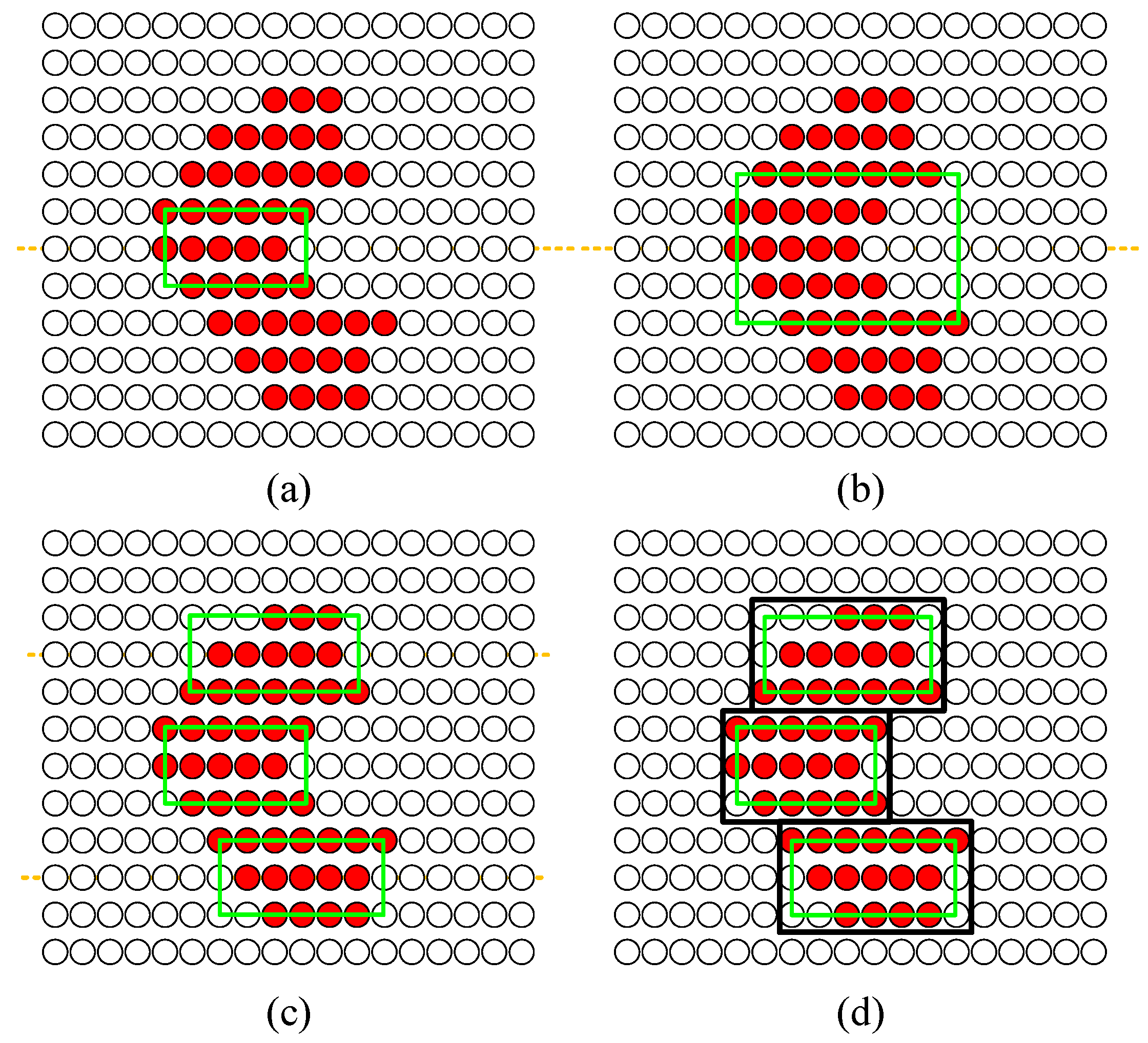
Figure 5 shows the construction of PolyBoundingBox, and tor is set to 70%. Figure 5a presents a watershed result colored in red, the middle line is found and drawn in a dashed orange line, the current minimum bounding box is constructed in a green box, and br = 88.9% that is bigger than tor. Figure 5b gives the next minimum bounding box of Figure 5a, and br = 66.7% that is smaller than tor. Hence, the current construction is finished, and the minimum bounding box in Figure 5a is selected. The other area is divided into two sub-areas, and the similar process is executed as shown in Figure 5c. The br is 71.4%, 88.9%, 76.2% from top to bottom that are both bigger than tor in Figure 5c. The expand result is presented in Figure 5d using the half length of the sampling interval, and colored in black boxes.
The preset value (tor) is critical for PolyBoundingBox construction. When using smaller tor, less poly lines are used to construct PolyBoundingBox roughly, which will introduce fewer control points and improve computational efficiency and vice versa. A proper value should be specified for PolyBoundingBox construction. Geometrical stage is executed since PolyBoundingBox is constructed.
3.2.2. Geometrical Stage of MSR Generation
The geometrical stage of MSR generation aims to calculate the Cartesian coordinate value of inserted control points using blending function refinement [8]. We denote T-spline surface before and after refinement as S and , which should satisfy the condition as follows:
Substituting Equation (1) into Equation (13), we have:
wherein, symbols without tilde represent the T-spline surface before refinement, and symbols with tilde represent the T-spline surface after refinement. Bi can be written as a linear combination of Bj based on blending function refinement as below:
Substituting Equation (15) into Equation (14), Equation (13) can be simplified:
in Equations (15) and (16) is calculated by means of blending function refinement that can be decomposed into the product of two B-spline basis function refinement. Cubic T-spline is considered in our research, and for each blending function in Equation (2), the B-spline basis function Ni(s) and Ni(t) are defined using five knots separately. Hence, there are four cases for B-spline basis function refinement as below.
We denote s = [s0, s1, s2, s3, s4] as knot vector for N(s) = N[s0, s1, s2, s3, s4](s) generally, and k is the knot that will be inserted.
− Insert k between s0 and s1.
− Insert k between s1 and s2.
− Insert k between s2 and s3.
− Insert k between s3 and s4.
If k < s0 or k > s4, N(s) does not change. The calculation of for blending function refinement can be derived by the refinement of Ni(s) and Ni(t). And the insertion of multiple knots can be performed by repeating the insertion of a single knot. Finally, the geometric information for control points that are used for MSRs construction can be obtained by solving Equation (16).
3.3. Optimized Multi-Rectangles Toolpath Generation for MSRs
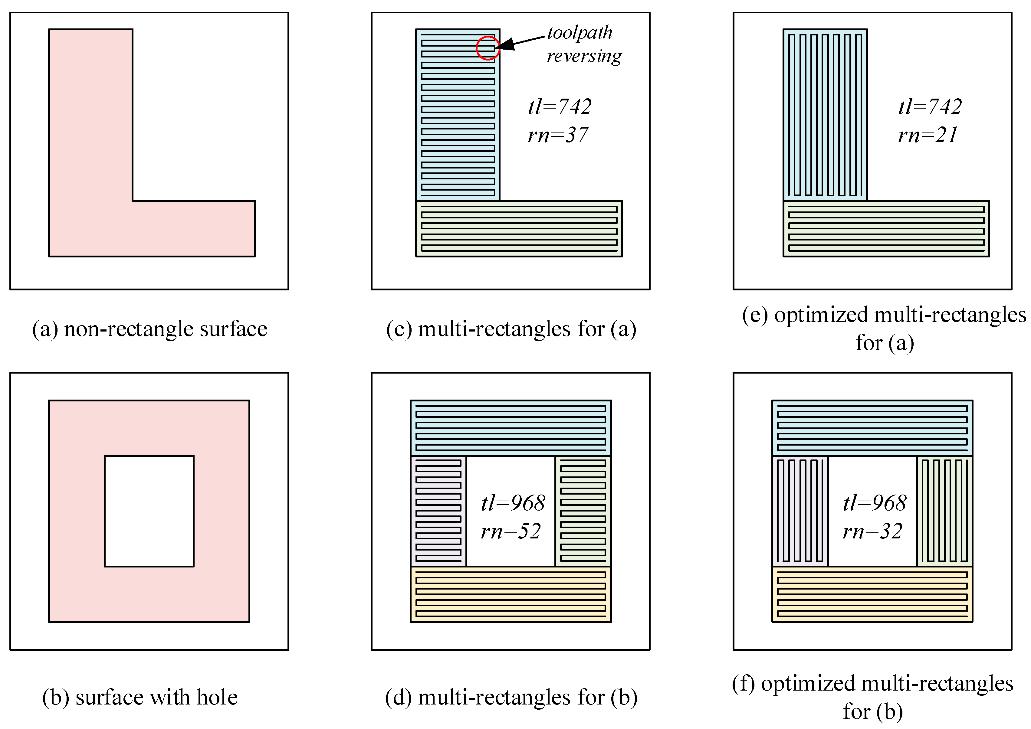
For the task of freeform surface finishing, UV strategy is usually adopted for freeform surface toolpath generation, various algorithms are developed based on UV strategy, such as iso-parametric, iso-scallop, iso-planar, and so on [4]. UV strategy consists of forward cutting and sideward cutting. The calculation of forward steps and sideward steps for a T-spline surface using a ball-end cutting tool can be found in our previous research [5]. UV strategy is convenient to implement for rectangular areas, which is efficient for a NURBS-represented freeform surface due to its rectangle parametric space. However, T-spline has the capability to describe a freeform surface with arbitrary parametric space using a single patch, including a non-rectangle surface and a surface with holes as shown in Figure 6a,b. Hence, it is not straightforward to introduce a UV strategy for the T-spline surface. In our previous research work [5], a multi-rectangles toolpath generation algorithm is presented for T-spline surface based on UV strategy. The T-spline surface can be decomposed into multi rectangles in parametric space, and UV strategies are adopted for each rectangular area intuitively as shown in Figure 6c,d.
Typically, UV strategy can generate two kinds of toolpath for the same area (U-direction and V-direction). The total length is almost the same for these two types of generated toolpath if the same parameters are employed. However, the reversing number of the cutting tool is totally different for these two types of toolpath, which has significant influence for machining time due to the acceleration and deceleration of the cutting tool near the reversing position. As shown in Figure 6, the reversing number is 37 and 52 in Figure 6c,d separately.
In our previous research work [5], the global UV strategy is used for each rectangular area to generate the toolpath, which cannot achieve the minimum reversing number. In the study, the type of UV strategy is considered for each rectangular area by means of the U-V ratio ruv that is defined in Equation (21), where lenu denotes the length of the rectangular area in U direction, and lenv denotes the similar meaning in V direction.
The lenu and lenv are calculated using Euclidean distance of the sampling points along U or V direction, as shown in Equation (22), where m and n are the number of sampling points along U and V direction.
If ruv is bigger than 1, U direction is selected for the forward step calculation of toolpath. If ruv is smaller than 1, V direction is selected for forward step calculation of toolpath. And if ruv is equal to 1, U and V direction can be selected arbitrarily for toolpath generation. After optimization, the total reversing number of cutting tool achieves the minimum for the whole T-spline surface. As shown in Figure 6e,f the reversing number is 21 and 32 separately.
4. Experiment and Discussion
The proposed method is tested using three T-spline surfaces as shown in Figure 7, Figure 8 and Figure 9. The proposed method is developed in the C++ programming language, which consists of watershed-based feature recognition, T-spline local refinement, and an optimized multi-rectangle toolpath generation algorithm. In the case study of the paper, br is set to be 0.5 for fewer control points insertion, and the iso-scallop strategy is employed for toolpath generation of each sub-region, chordal tolerance and scallop height are set to be 0.1 mm respectively.
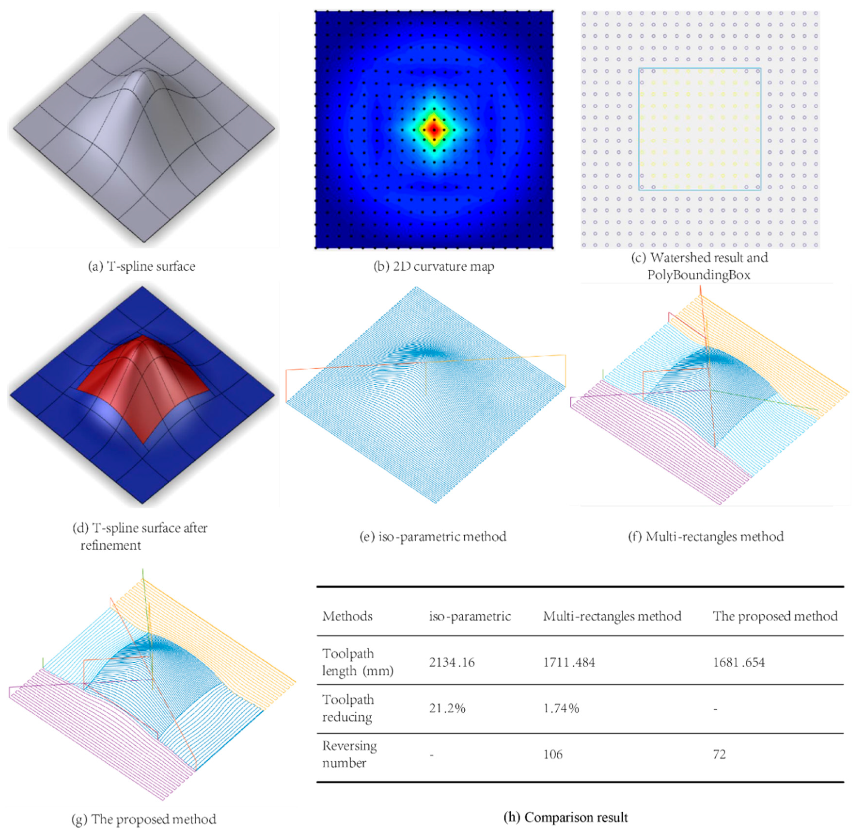
The first test surface demonstrates the basic processing of our proposed method. The surface has one convex feature as shown in Figure 7a, 2DCM is displayed in Figure 7b with 20 by 20 sampling, in Figure 7c, the convex feature is recognized using watershed technology and colored by yellow points, the PolyBoundingBox is also constructed in Figure 7c, Figure 7d presents the T-spline surface after local refinement, and the convex feature is defined by a set of faces colored in red. For comparison, a toolpath is generated by using the iso-parametric method, multi-rectangle method and our proposed method as shown in Figure 7e–g, and the result is given in Figure 7h. The proposed method can reduce the toolpath by about 21.2% in contrast to the iso-parametric method, and is almost the same in comparison with multi-rectangles method. However, our proposed method has a toolpath with a lower reversing number that can reduce the number of accelerations and decelerations for machining.
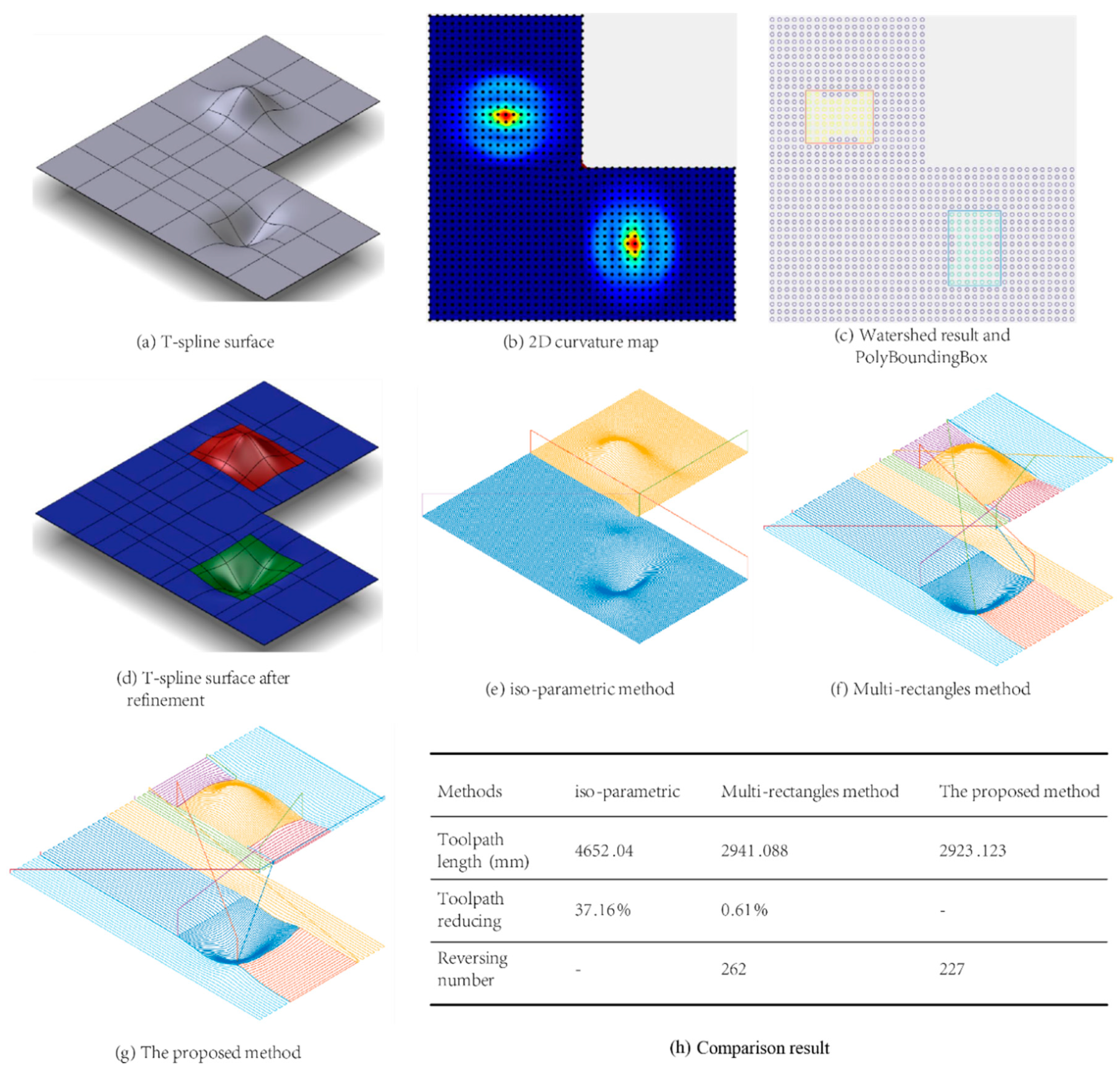
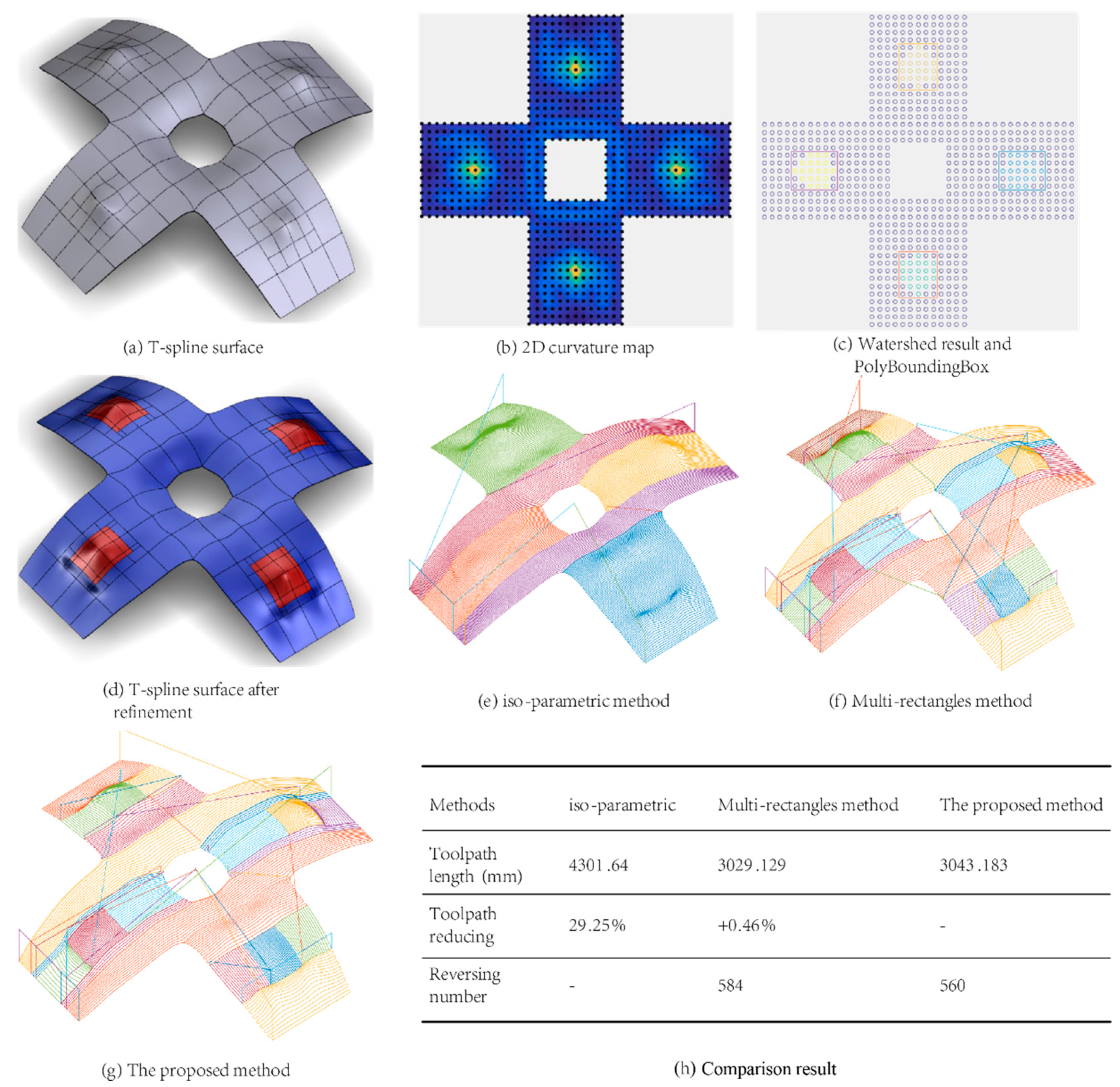
The second and third test surfaces are much more complicated than the first one. The second one is a non-rectangle surface without holes, and has one convex feature and one concave feature. The third one is a non-rectangle surface with one hole, and has four convex features. In Figure 8 and Figure 9 are presented (a) the original T-spline surface; (b) a two-dimensional curvature map of the surface shaded by root mean square curvature; (c) the watershed result of the surface and PolyBoundingBox construction for convex and concave sub-regions; (d) T-spline surface after local refinement, with the convex sub-region shaded in red, the concave sub-region shaded in green, and other sub-regions shaded in blue; (e) toolpath generation for the surface using the iso-parametric method; (f) toolpath generation for the surface using the multi-rectangles method; (g) toolpath generation for the surface using our proposed method; (h) the comparison results of toolpath length and reversing number for three toolpath generation methods.
The proposed method can decrease toolpath length significantly relative to the iso-parametric method, and the toolpath length is almost the same in comparison with the multi-rectangle method. However, the toolpath reversing number of our proposed method is less than the multi-rectangle method, which can save machining costs and improve the stability of machine tool. The boundaries of sub-regions can be defined mathematically based on T-spline local refinement, and the continuity near the sub-regions is guaranteed with the help of T-spline properties.
Machining time is one of the key metrics for freeform surface finishing. Machining simulation is carried out to demonstrate the advantage of our proposed method. NX manufacturing is a powerful software for machine tool simulation, and we have carried out the cutting simulation and listed the machining time in Table 1. The virtual machine is SIM01 Mill 3ax Fanuc (millimeter), the feed speed is 1000 mm/min, the acceleration and deceleration of the cutting tool is controlled by the NCK (Numerical Control Kernel) of Siemens.
There are deviations between simulation and real cutting because of the stock material, cutting tool, machine tool parameters (especially the motor parameters), approach and retract strategy, and so on. However, the simulation results also show that our proposed method has an advantage compared with the other two methods for machining time.
5. Conclusions
A region-based toolpath generation method for a T-spline surface is presented based on watershed technology in this report. The region-based method is one of the most efficient approaches for the toolpath generation of a freeform surface to achieve constant scallop over the whole surface. However, NURBS is not the ideal tool for freeform surface representation due to the gaps involved near the segmented boundaries of sub-regions. Hence, T-spline is introduced to describe freeform surface, with the capability to segment a freeform surface into a set of gap-free sub-regions. In order to divide the freeform surface while preserving features, we extend watershed technology for freeform surface segmentation because of its robustness and efficiency in the field of image processing and mesh segmentation, wherein 2DCM is constructed based on T-spline sampling to carry out watershed-based feature recognition. T-spline local refinement is adopted near segmented boundaries of sub-regions to construct MSRs that are convenient for toolpath generation. For MSR construction of sub-regions, the PolyBoundingBox is proposed to process topological insertion of control points, and blending function refinement is introduced for geometrical calculation of inserted points. Lastly, an optimized multi-rectangle toolpath generation algorithm is presented, which can obtain the minimum reversing number for a cutting tool for a segmented T-spline surface. Compared to traditional methods, the proposed method shows the feasibility and efficiency for toolpath generation of a T-spline surface.
6. Future Work
The contour parallel toolpath has advantages for toolpath reversing, whereas the toolpath on the corner should be processed further, and the smoothing method should be considered for arbitrary T-spline surface. The spiral toolpath method for T-spline surface is considered for our next research, and the comparison between UV strategy and spiral strategy for the T-spline surface will be reported in our future research.
Author Contributions
Y.L. proposes the main idea and realize the system. G.Z. and P.H. provide many suggestions about the innovations and the paper revision. All authors have read and agreed to the published version of the manuscript.
Funding
This research was funded by Natural Science Foundation of China, grant number 61572056.
Acknowledgments
The author would like to express their sincere thanks to the supports of the Natural Science Foundation of China (No. 61572056).
Conflicts of Interest
The authors declare no conflict interest.
References
- Liu, X.-W. Five-axis NC cylindrical milling of sculptured surfaces. Comput. Des. 1995, 27, 887–894. [Google Scholar] [CrossRef]
- Au, C. A path interval generation algorithm in sculptured object machining. Int. J. Adv. Manuf. Technol. 2001, 17, 558–561. [Google Scholar] [CrossRef]
- Tournier, C.; Duc, E. A surface based approach for constant scallop heighttool-path generation. Int. J. Adv. Manuf. Technol. 2002, 19, 318–324. [Google Scholar] [CrossRef] [Green Version]
- Lasemi, A.; Xue, D.; Gu, P. Recent development in CNC machining of freeform surfaces: A state-of-the-art review. Comput. Des. 2010, 42, 641–654. [Google Scholar] [CrossRef]
- Zhao, G.; Liu, Y.; Xiao, W.; Zavalnyi, O.; Zheng, L. STEP-compliant CNC with T-spline enabled toolpath generation capability. Int. J. Adv. Manuf. Technol. 2017, 94, 1799–1810. [Google Scholar] [CrossRef]
- Liu, Y.; Zhao, G.; Zavalnyi, O.; Xiao, W. Toolpath generation for partition machining of T-spline surface based on local refinement. Int. J. Adv. Manuf. Technol. 2019, 102, 3051–3064. [Google Scholar] [CrossRef]
- Liu, Y.; Zhao, G.; Zavalnyi, O.; Xiao, W. STEP-NC compliant data model for freeform surface manufacturing based on T-spline. Int. J. Comput. Integr. Manuf. 2019, 32, 979–995. [Google Scholar] [CrossRef]
- Sederberg, T.W.; Cardon, D.L.; Finnigan, G.T.; North, N.S.; Zheng, J.; Lyche, T. T-spline simplification and local refinement. ACM Trans. Graph. 2004, 23, 276. [Google Scholar] [CrossRef] [Green Version]
- Sederberg, T.W.; Zheng, J.; Bakenov, A.; Nasri, A.H. T-splines and T-NURCCs. ACM Trans. Graph. 2003, 22, 477. [Google Scholar] [CrossRef]
- Verma, A.K.; Rajotia, S. A review of machining feature recognition methodologies. Int. J. Comput. Integr. Manuf. 2010, 23, 353–368. [Google Scholar] [CrossRef]
- Zhang, X.; Wang, J.; Yamazaki, K.; Mori, M. A surface based approach to recognition of geometric features for quality freeform surface machining. Comput. Des. 2004, 36, 735–744. [Google Scholar] [CrossRef]
- Sheen, B.-T.; You, C.-F. Machining feature recognition and tool-path generation for 3-axis CNC milling. Comput. Des. 2006, 38, 553–562. [Google Scholar] [CrossRef]
- Sunil, V.; Pande, S. Automatic recognition of features from freeform surface CAD models. Comput. Des. 2008, 40, 502–517. [Google Scholar] [CrossRef]
- Zhang, C.; Zhou, X.; Li, C. Feature extraction from freeform molded parts for moldability analysis. Int. J. Adv. Manuf. Technol. 2009, 48, 273–282. [Google Scholar] [CrossRef]
- Wang, J.; Wang, Z.; Zhu, W.; Ji, Y. Recognition of freeform surface machining features. J. Comput. Inf. Sci. Eng. 2010, 10, 041006. [Google Scholar] [CrossRef]
- Gupta, R.K.; Gurumoorthy, B. Automatic extraction of free-form surface features (FFSFs). Comput. Des. 2012, 44, 99–112. [Google Scholar] [CrossRef]
- Li, Y.; Wang, W.; Liu, X.; Ma, Y. Definition and recognition of rib features in aircraft structural part. Int. J. Comput. Integr. Manuf. 2013, 27, 1–19. [Google Scholar] [CrossRef]
- Liu, X.; Li, Y.; Gao, J. A multi-perspective dynamic feature concept in adaptive NC machining of complex freeform surfaces. Int. J. Adv. Manuf. Technol. 2015, 82, 1259–1268. [Google Scholar] [CrossRef]
- Meyer, F. Topographic distance and watershed lines. Signal Process. 1994, 38, 113–125. [Google Scholar] [CrossRef]
- Mangan, A.; Whitaker, R. Partitioning 3D surface meshes using watershed segmentation. IEEE Trans. Vis. Comput. Graph. 1999, 5, 308–321. [Google Scholar] [CrossRef] [Green Version]
- Pulla, S.; Razdan, A.; Farin, G. Improved curvature estimation for watershed segmentation of 3-dimensional meshes. IEEE Trans. Vis. Comput. Graph. 2001, 5, 308–321. [Google Scholar]
- Koschan, A. Perception-based 3D triangle mesh segmentation using fast marching watersheds. In Proceedings of the CVPR 2003 Computer Vision and Pattern Recognition Conference, Madison, WI, USA, 18–20 June 2003; Institute of Electrical and Electronics Engineers (IEEE): Madison, WI, USA, 2003. [Google Scholar]
- Wu, F.-C.; Chen, B.-Y.; Liang, R.-H.; Ouhyoung, M. Prong features detection of a 3D model based on the watershed algorithm. In Proceedings of the SIGGRAPH’04, Los Angeles, CA, USA, 8–12 August 2004; Association for Computing Machinery: New York, NY, USA, 2004. [Google Scholar]
- Romstad, B.; Etzelmüller, B. Mean-curvature watersheds: A simple method for segmentation of a digital elevation model into terrain units. Geomorphology 2012, 139, 293–302. [Google Scholar] [CrossRef] [Green Version]
- Čomić, L.; De Floriani, L.; Iuricich, F.; Magillo, P. Computing a discrete Morse gradient from a watershed decomposition. Comput. Graph. 2016, 58, 43–52. [Google Scholar] [CrossRef] [Green Version]
- Delest, S.; Boné, R.; Cardot, H. 3D watershed transformation based on connected faces structure. CompIMAGE 2006, 6, 159–163. [Google Scholar]
Figure 1.
Knot vectors calculation, influence domain, influence points of T-spline surface: (a) Knot vectors calculation of control points using the ray intersection method, (b) the influence domain of a control point filled with shaded area, (c) a set of control points marked by a solid circle for one shaded face.

Figure 2.
Flow chart of watershed-based toolpath generation for the T-spline surface: (a) the input T-spline surface that has one convex feature, (b) two-dimensional curvature map shaded by root-mean-square curvature, (c) watershed results and PolyBoundingBox construction for the convex feature, (d) MSRs generation using T-spline local refinement, and sub-regions are shaded using different color, (e) optimized multi-rectangle toolpath generation for the surface.

Figure 3.
The two-dimensional curvature map (2DCM) of the T-spline surface.

Figure 4.
Feature recognition using watershed technology.

Figure 5.
An example of PolyBoundingBox construction for watershed result. From (a–d) show the construction of PolyBoundingBox.
Figure 5.
An example of PolyBoundingBox construction for watershed result. From (a–d) show the construction of PolyBoundingBox.

Figure 6.
Optimized multi-rectangle algorithm, tl denotes the total length of toolpath, and rn denotes the revering number of toolpath.
Figure 6.
Optimized multi-rectangle algorithm, tl denotes the total length of toolpath, and rn denotes the revering number of toolpath.

Figure 7.
Demonstration and comparison of watershed-based toolpath generation of T-spline surface 1.
Figure 7.
Demonstration and comparison of watershed-based toolpath generation of T-spline surface 1.

Figure 8.
Demonstration and comparison of watershed-based toolpath generation of T-spline surface 2.
Figure 8.
Demonstration and comparison of watershed-based toolpath generation of T-spline surface 2.

Figure 9.
Demonstration and comparison of watershed-based toolpath generation of T-spline surface 3.
Figure 9.
Demonstration and comparison of watershed-based toolpath generation of T-spline surface 3.


Table 1.
Machining time of toolpath simulation.
| Machining Time (min:sec) | iso-Parametric | Multi-Rectangle Method | The Proposed Method |
|---|---|---|---|
| T-spline surface 1 | 3:26 | 10:49 | 11:48 |
| T-spline surface 2 | 2:47 | 6:01 | 6:54 |
| T-spline surface 3 | 2:30 | 5:22 | 6:31 |
© 2020 by the authors. Licensee MDPI, Basel, Switzerland. This article is an open access article distributed under the terms and conditions of the Creative Commons Attribution (CC BY) license (http://creativecommons.org/licenses/by/4.0/).
Share and Cite
MDPI and ACS Style
Liu, Y.; Zhao, G.; Han, P. T-Spline Surface Toolpath Generation Using Watershed-Based Feature Recognition. Appl. Sci. 2020, 10, 6790. https://doi.org/10.3390/app10196790
AMA Style
Liu Y, Zhao G, Han P. T-Spline Surface Toolpath Generation Using Watershed-Based Feature Recognition. Applied Sciences. 2020; 10(19):6790. https://doi.org/10.3390/app10196790
Chicago/Turabian StyleLiu, Yazui, Gang Zhao, and Pengfei Han. 2020. "T-Spline Surface Toolpath Generation Using Watershed-Based Feature Recognition" Applied Sciences 10, no. 19: 6790. https://doi.org/10.3390/app10196790
Note that from the first issue of 2016, this journal uses article numbers instead of page numbers. See further details here.