Safety Issues Referred to Induced Sheath Voltages in High-Voltage Power Cables—Case Study


Faculty of Electrical and Control Engineering, Gdańsk University of Technology, Narutowicza 11/12, PL-80-233 Gdańsk, Poland
*
Author to whom correspondence should be addressed.
Appl. Sci. 2020, 10(19), 6706; https://doi.org/10.3390/app10196706
Submission received: 20 August 2020
/
Revised: 7 September 2020
/
Accepted: 23 September 2020
/
Published: 25 September 2020
(This article belongs to the Special Issue Electrical Safety Engineering of Complex Systems)
Abstract
:Load currents and short-circuit currents in high-voltage power cable lines are sources of the induced voltages in the power cables’ concentric metallic sheaths. When power cables operate with single-point bonding, which is the simplest bonding arrangement, these induced voltages may introduce an electric shock hazard or may lead to damage of the cables’ outer non-metallic sheaths at the unearthed end of the power cable line. To avoid these aforementioned hazards, both-ends bonding of metallic sheaths is implemented but, unfortunately, it leads to increased power losses in the power cable line, due to the currents circulating through the sheaths. A remedy for the circulating currents is cross bonding—the most advanced bonding solution. Each solution has advantages and disadvantages. In practice, the decision referred to its selection should be preceded by a wide analysis. This paper presents a case study of the induced sheath voltages in a specific 110 kV power cable line. This power cable line is a specific one, due to the relatively low level of transferred power, much lower than the one resulting from the current-carrying capacity of the cables. In such a line, the induced voltages in normal operating conditions are on a very low level. Thus, no electric shock hazard exists and for this reason, the simplest arrangement—single-point bonding—was initially recommended at the project stage. However, a more advanced computer-based investigation has shown that in the case of the short-circuit conditions, induced voltages for this arrangement are at an unacceptably high level and risk of the outer non-metallic sheaths damage occurs. Moreover, the induced voltages during short circuits are unacceptable in some sections of the cable line even for both-ends bonding and cross bonding. The computer simulations enable to propose a simple practical solution for limiting these voltages. Recommended configurations of this power cable line—from the point of view of the induced sheath voltages and power losses—are indicated.
1. Introduction
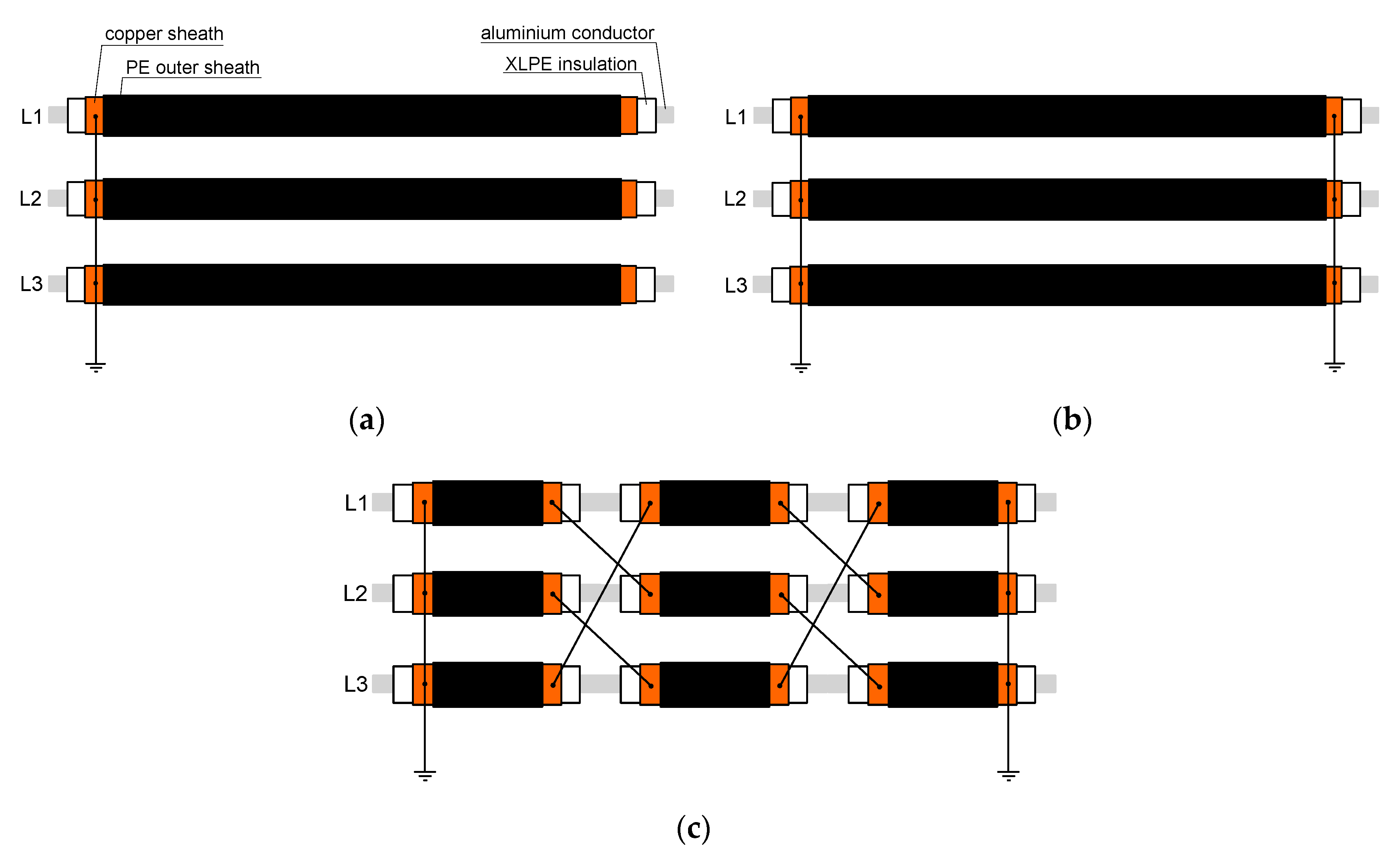
High-voltage transmission and distribution power lines are usually used overhead with bare conductors. The main reason for the widespread use of overhead power lines, instead of cable lines, is their lower investment cost. However, there are cases in which the application of overhead lines is precluded. These refer mainly to urban areas but also to rural areas when an increased risk of electric shock hazard or exposure to electromagnetic fields exists [1]. With many undoubtable advantages, the utilization of high-voltage cable lines is associated with some problems. One of the main problems is the induced voltage generated in the power cable’s metallic concentric sheath. With reference to this voltage, power cables may operate as single-point bonded, both-ends bonded or cross-bonded. Recommendations for the performance of power cables bonding and earthing are mainly included in the standards [2,3] as well as the report [4]. Figure 1 presents the three aforementioned cable bonding arrangements.
The simplest cable sheath bonding arrangement is single-point bonding. In such a solution (Figure 1a) the load current in the cable conductor (core) induces a voltage in the sheath, which value is the highest at the unearthed end of the power cable line. The induced sheath voltages for any cables’ formation in a single-circuit system can be calculated (in simplified form) as follows [2]:
where: VL1-sh, VL2-sh, VL3-sh are the induced sheath voltages (V/m) in phases L1, L2 and L3, respectively; IL1, IL2, IL3, are the load currents in the cable conductor (core) of phases L1, L2 and L3, respectively; Dcu is the geometric mean sheath diameter; DL1-L2 is the axial spacing of phases L1 and L2; DL2-L3 is the axial spacing of phases L2 and L3; DL1-L3 is the axial spacing of phases L1 and L3.
For more accurate calculation of the voltages, especially taking into account the electromagnetic couplings, computer-based tools should be employed. The computer-aided modelling of the induced sheath voltages with the use of the PSCAD/EMTDC software is presented in [5], whereas [6] presented the calculation by the Pearson Correlation. Multiple-circuit systems require the application of advanced computer-based tools to calculate these voltages, as presented by the authors in [7] or other researchers in [8,9].
To avoid electric shock, the induced voltage-to-earth at the unearthed end should not exceed permissible values determined by the standard [10]. For a long-time of touch voltage duration, the permissible value is equal to 80 V. When the load current is relatively low or a cable line is not long, values of the induced voltages are usually below the permissible limit. A more serious problem occurs in the case of a line-to-earth fault at the unearthed end. If the value of the short-circuit current is high, this current produces a high-value induced voltage, which may damage the cables’ non-metallic polyethylene (PE) outer sheath. It is assumed in the engineering practice that during the short-circuit conditions the induced voltage should not exceed 5 kV. To limit values of the induced voltage, an earth continuity conductor (ECC) is buried in the ground, parallel to the cables, what was widely studied in [11]. The extensive analysis conducted in [12] shows that in special cases the ECC may reduce the induced voltages by even over 60% compared to a system without the ECC. Despite this, the induced voltages may still exceed the acceptable level. Moreover, the study results presented in [13] indicate that in the case of the uninsulated ECC, dangerous touch voltages may appear around this parallel cable. For these reasons or when the voltages are too high in normal operating conditions, both-ends bonding of cables is used as an alternative (Figure 1b).
When both-ends bonding is used, metallic sheaths are bonded and earthed in the accessible points in substations and no risk of electric shock occurs in normal operating conditions. Moreover, in the case of a line-to-earth short circuit, the current distribution through the earthing system is more favourable [14], especially when a global earthing system exists in the analyzed area [15]. The most unfavourable effect of the both-ends bonding is the presence of sheath circulating currents. These currents produce additional power losses in the cables and hence decrease the current-carrying capacity. Such power losses, due to the induced voltages, may occur even in HVDC power cable systems, as underlined in [16]. Therefore, it is important to evaluate sheath circulating currents with relatively high accuracy [17], taking into account different geometries of the cables [18], sheath resistance, phase rotation and cable armouring [19] as well as varied load conditions [20]. High circulating currents and high power losses resulting from them are required to be reduced [21,22,23,24]. The most effective method of sheath currents suppression, but relatively complicated, is the implementation of the cross-bonded cable system (Figure 1c). Broad studies of this method are included in [25,26,27,28,29,30]. Transposition of the cables’ sheaths in particular phases compensates induced voltages and theoretically, no production of the sheath circulation currents occurs.
The literature study leads to the conclusion that methods of the induced sheath voltages and sheath circulating currents reduction should be applied very carefully. Any given cable system, especially a complicated one, should always be analyzed individually. Unfortunately, the selection of the type of bonding in the particular case of the cable system is not an easy task. In practice, a compromise between technical and economic aspects should be reached.
This paper presents a comprehensive study of the induced voltages in the 110 kV power cable line. The power cable line is relatively long (12 km) but the power transferred via this line is very low (approx. 12% with reference to max permissible power transfer via the cables) due to a specific type of the industrial consumer at the end of the line. Such a low transferred power suggests the application of the single-point bonding in the analyzed power cable line because the induced sheath voltages at the unearthed end are clearly below the permissible limit equal to 80 V, hence no electric shock hazard exists. However, the short-circuit analysis has shown that the single-point bonding is excluded—very high values of the induced voltages are dangerous for the non-metallic PE outer sheath. The results of the calculations suggest to apply both-ends bonding or cross bonding, but detailed analysis for these arrangements has shown that the risk of outer sheath damage still exists in some sections of the power cable line. A solution for the elimination of too high induced voltages during a short circuit is indicated.
As an extension of the analysis related to induced voltages, power losses in the cable system, including in cables’ sheaths, have been calculated for all types of bonding. In some cases, values of the power losses may be a decisive factor in selecting the type of the bonding system.
The presented results of the analysis of the induced voltages and power losses in the example high-voltage power cable line can be useful for practical applications, especially for the designers of the cable lines. The analysis has indicated the possible critical/weak points in such lines, which could be overlooked at the design stage.
2. Description of the Analyzed 110 kV Cable Line
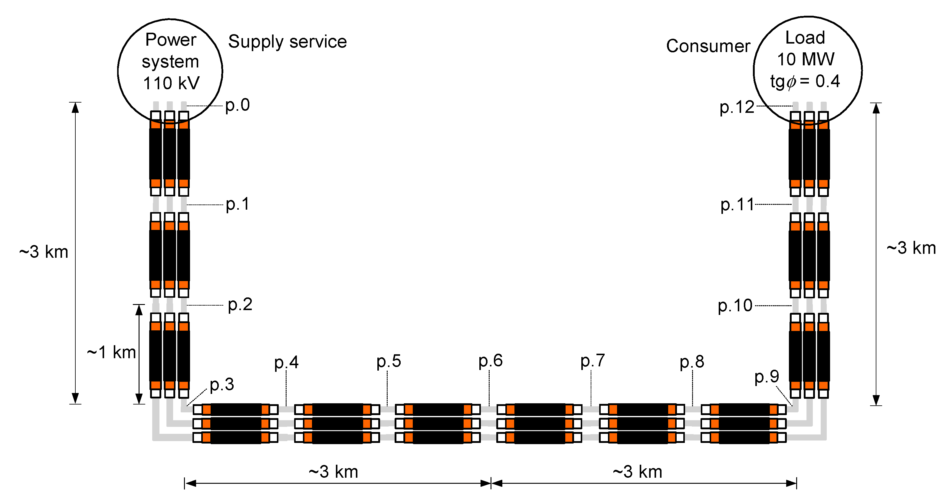
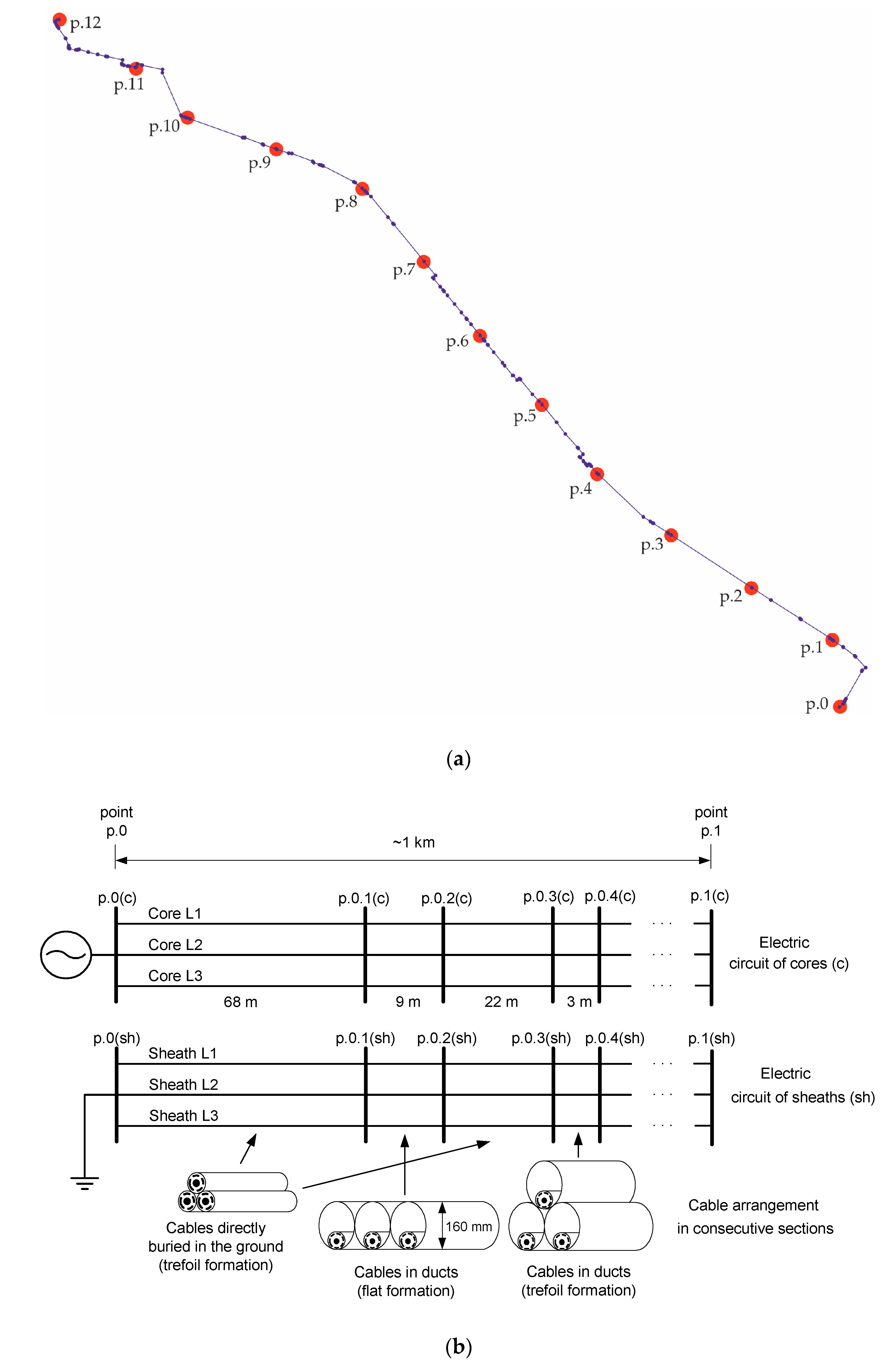
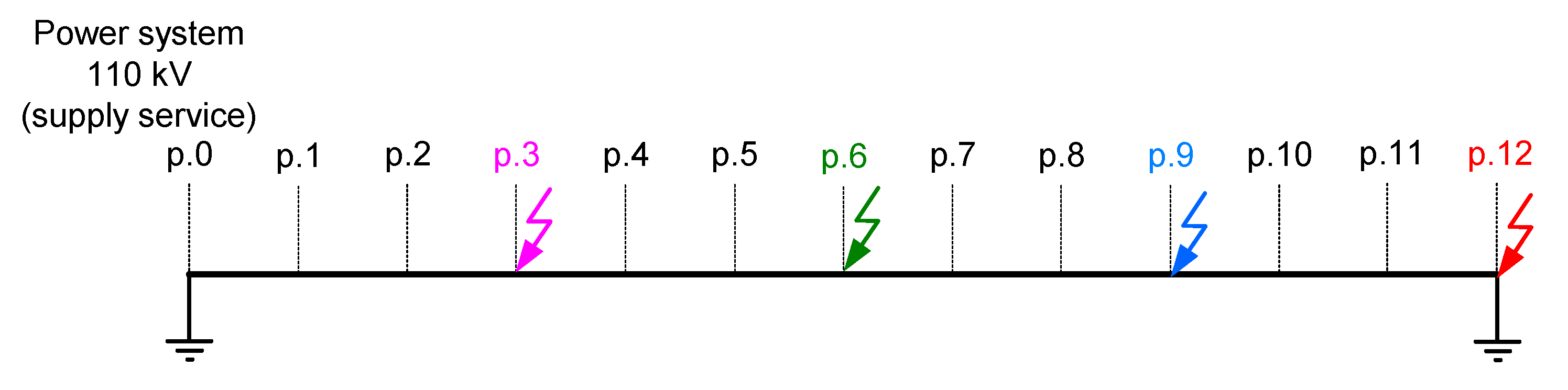
The power cable system under analysis connects a 110 kV power substation (supply service) and a dedicated consumer/load (Figure 2). The total length of the single-circuit three-phase cable line is approx. 12 km. The manufacturer’s length of the cable (minor section) is equal to approx. 1 km and the points with connections of the consecutive sections are marked p.0–p.12 in Figure 2. In some of these points, earthing and bonding (including cross bonding) of the cables’ sheaths are possible. Generally, cables are laid in trefoil formation without spacing. Some spacing, as well as short sections with flat formation, are applied in the cable ducts, what is included in the computer model.
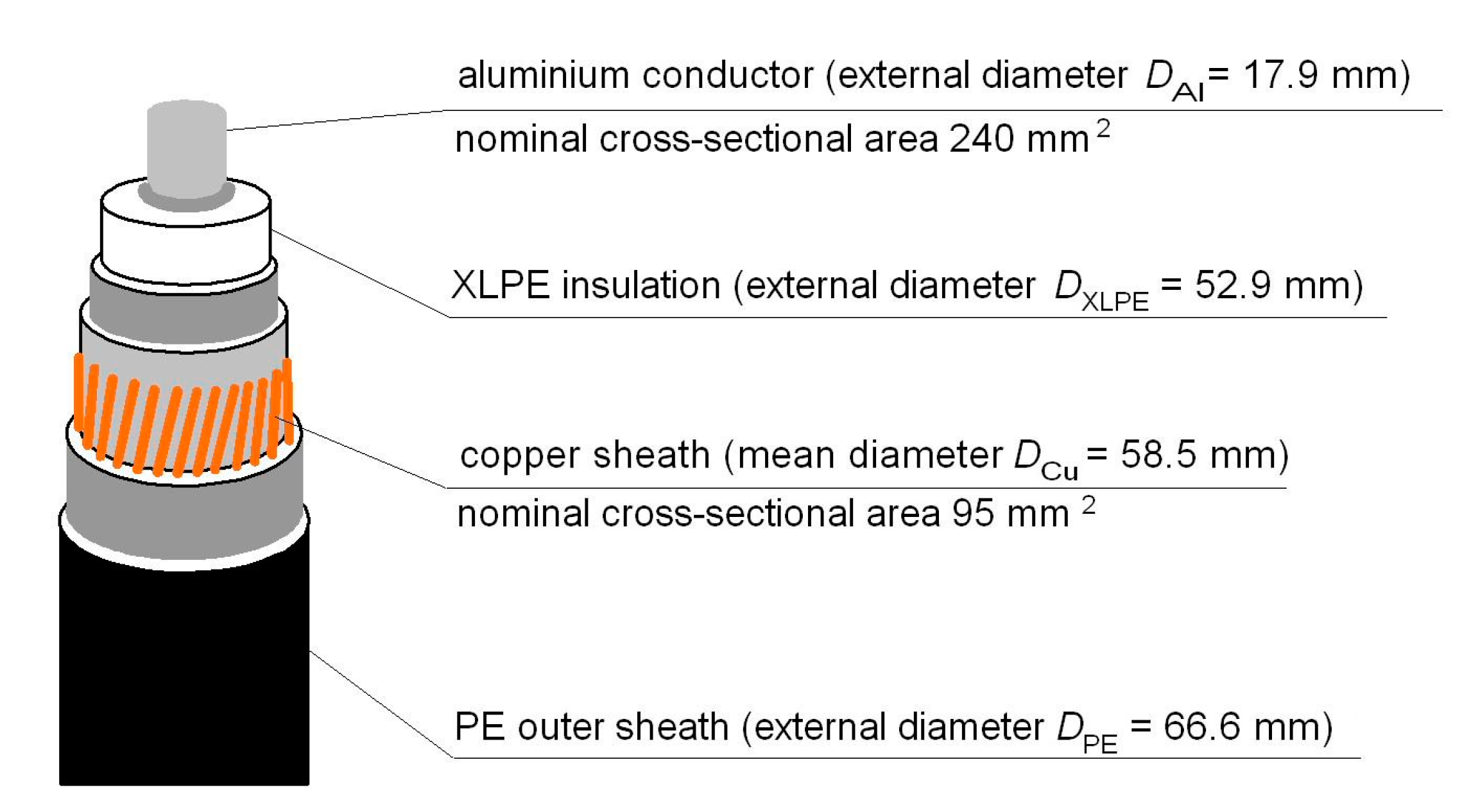
The type of cable used in this line is presented in Figure 3 (a simplified view). The nominal parameters of the cable/cable line are as follows [31]:
- nominal voltage of the cable: 110 kV (line-to-line), 64 kV (line-to-earth);
- nominal cross-sectional area of the aluminium conductor (core): 240 mm2; (external diameter DAl = 17.9 mm);
- resistance of the aluminum conductor (core): 0.125 Ω/km (DC in 20 °C), 0.161 Ω/km (AC in max temp. 90 °C);
- nominal cross-sectional area of the copper sheath: 95 mm2 (mean diameter DCu = 58.5 mm);
- resistance of the copper sheath: 0.192 Ω/km (DC in 20 °C);
- inductive reactance of the cable line in the trefoil formation: 0.143 Ω/km;
- XLPE insulation external diameter: DXLPE = 52.9 mm;
- PE outer sheath external diameter (the outer diameter of the cable): DPE = 66.6 mm;
- the current-carrying capacity in the trefoil formation: 421 A (single-point bonding), 409 A (both-ends bonding);
- short-circuit power at the supply service point: 1120 MVA.
On the base of the nominal parameters of the cable/cable line, it can be stated that the maximum permissible power transmitted via this line is approx. 80 MW. However, the consumer’s demand is only 10 MW and the connection of other loads to this 110 kV cable line is not planned.
The power cable system under analysis has been modelled with the use of the PowerFactory software [32]. The computer model takes into account all data delivered by the investor, among other: cable technical parameters, cable line layout (including the arrangement with cable ducts), possible points of the bonding or earthing. The entire model of the line consists of 161 sections, of which 61 are cable ducts with different cable arrangements. Two types of cable ducts are used: the flat formation and the trefoil formation. The participation of the flat formation ducts in the length of the line is 1.7%, and the participation of the trefoil formation ducts is 8.2%. Thus, 90% of the cable line length is the trefoil formation without spacing and without ducts—for rough calculations of the induced voltages, it is acceptable to assume such a formation along the entire length of the line.
Figure 4a presents a cable route, which is reflected in the computer model—small blue dots indicate a change in cable spacing (due to ducts application). The cables’ joints are marked as big red dots.
The PowerFactory software allows for modelling cable lines, including cable spacing, which means that the software automatically determines the selected power line electrical parameters. Impedance Z and admittance Y of cables are defined in two matrix equations presented in [33] and implemented in the software as well as described in its guide [34]:
where: |V| and |I| are the voltage and current vectors respectively, at distance x along the cable line; |Z| and |Y| are square matrices of the impedance and admittance respectively.
The complexity of |Z| and |Y| matrices depends on the number of cables and the number of layers per single cable. The impedance and admittance matrices can be described in the following way:
where: the matrices with subscript i include cable parameters (core, sheath and armour); the matrices with subscript 0 include parameters of the cable outer media (air, earth); the matrices with subscripts p and c include parameters of a pipe (an enclosure—if applied); C is a potential coefficient matrix; s = jω.
Detailed information on the calculation of individual components of the impedance and admittance matrices can be found in [33,34].
In the considered case, the cable line model consists of two electromagnetically coupled circuits: cores electric circuit (c) and sheaths electric circuit (sh) (Figure 4b). The results of the multi-variant computer analysis included in the next sections show the levels of voltages induced in the cables’ sheaths and risks referred to them, as well as the power losses influencing the current-carrying capacity of the cables.
3. Results of the Induced Voltages Computer Simulations
3.1. Induced Voltages for Single-Point Bonding
In the first stage of the analysis, the induced sheath voltages in normal operating conditions, in case of the single-point bonding, have been analyzed. The load current flow in the cable cores, as well as the induced voltages, are calculated by the software taking into account the electromagnetic couplings. All charts presenting the induced voltages include the highest rms values among phases L1, L2, L3.
The analyses have been conducted for the following variables:
- the transferred power equal to 1 MW (an example very low power), 10 MW (contracted/declared consumed power), 80 MW (maximal permissible power in terms of the current-carrying capacity of the cables; a theoretical value, used for the comparison purposes);
- the reactive-to-active power ratio: tgϕ = Q/P = 0 or tgϕ = Q/P = 0.4 (contracted).
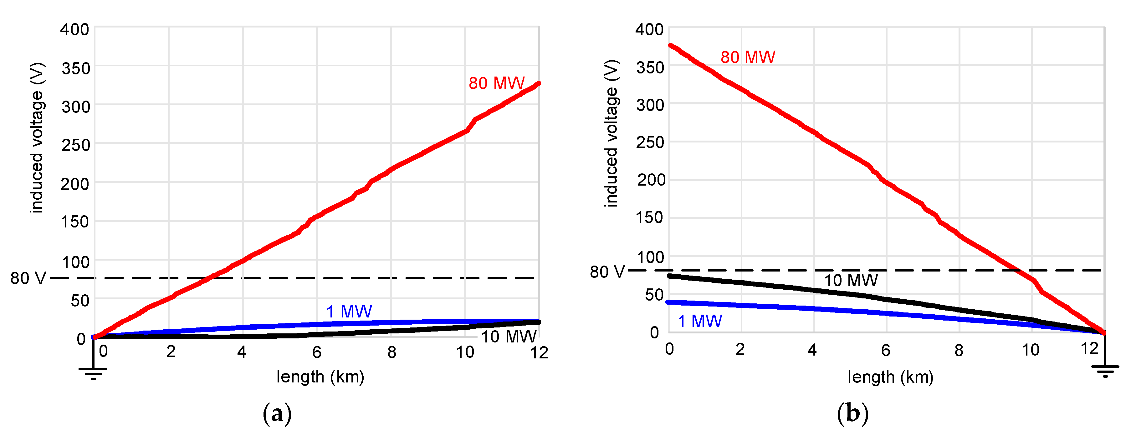
Figure 5 presents the induced sheath voltages for the case with the tgϕ = 0. When the single-point bonding is performed at the 110 kV supply service substation (Figure 5a), the induced voltages are significantly below the assumed limit 80 V indicated in the standard [10], both for the power 1 MW and the contracted power 10 MW. The value 80 V is many times exceeded in the case of the 80 MW (approx. 330 V), but it is presented only for the comparison purposes. When the single-point bonding is performed at the consumer substation (Figure 5b), the induced voltages are generally higher than for the case presented in Figure 5a. For the transferred power 10 MW, it is close to the permissible limit 80 V at the unearthed end of the line (point p.0).
The differences in the induced voltages (Figure 5a vs. Figure 5b) are the effect of the natural load of the cable line (capacitive), which forces a capacitive current flow of a changing value along the length of the cable line. It indicates that the location of the point of the earthing (reference point) is important. Note, that for the case presented in Figure 5a, the induced voltages at the unearthed end are practically the same for the power 1 MW and 10 MW. In the case of Figure 5b, the respective voltages at the unearthed end differ about two times.
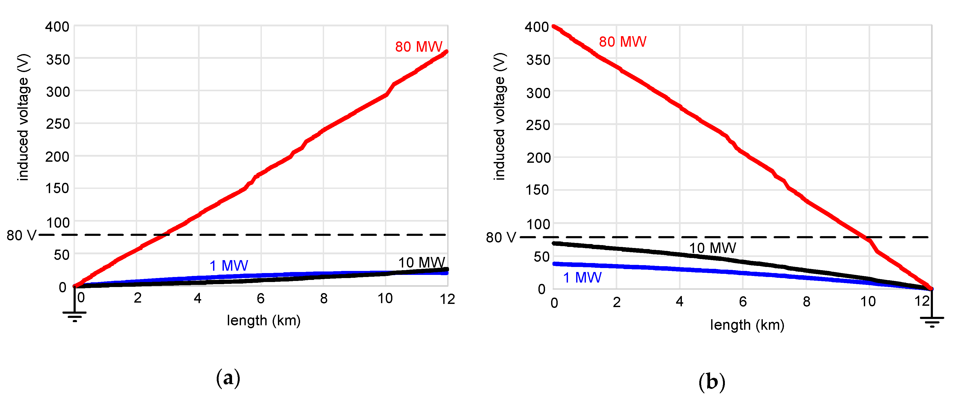
Similar general conclusions flow from the analysis of the results presented in Figure 6 (tgϕ = 0.4). However, the variations of the induced voltages along the length of the cable line are slightly different than for the tgϕ = 0, especially if one compares Figure 5a vs. Figure 6a for 1 MW and 10 MW. Thus, the reactive-to-active power ratio tgϕ, natural capacitive power of the cables as well as the location of the point of the single-point bonding and earthing should be taken into account in the safety analysis. In the light of the aforementioned investigation, it can be concluded that for the contracted transferred power (10 MW, tgϕ = 0.4), the single-point bonding is acceptable, whether in p.0 (preferred) or in p.12.
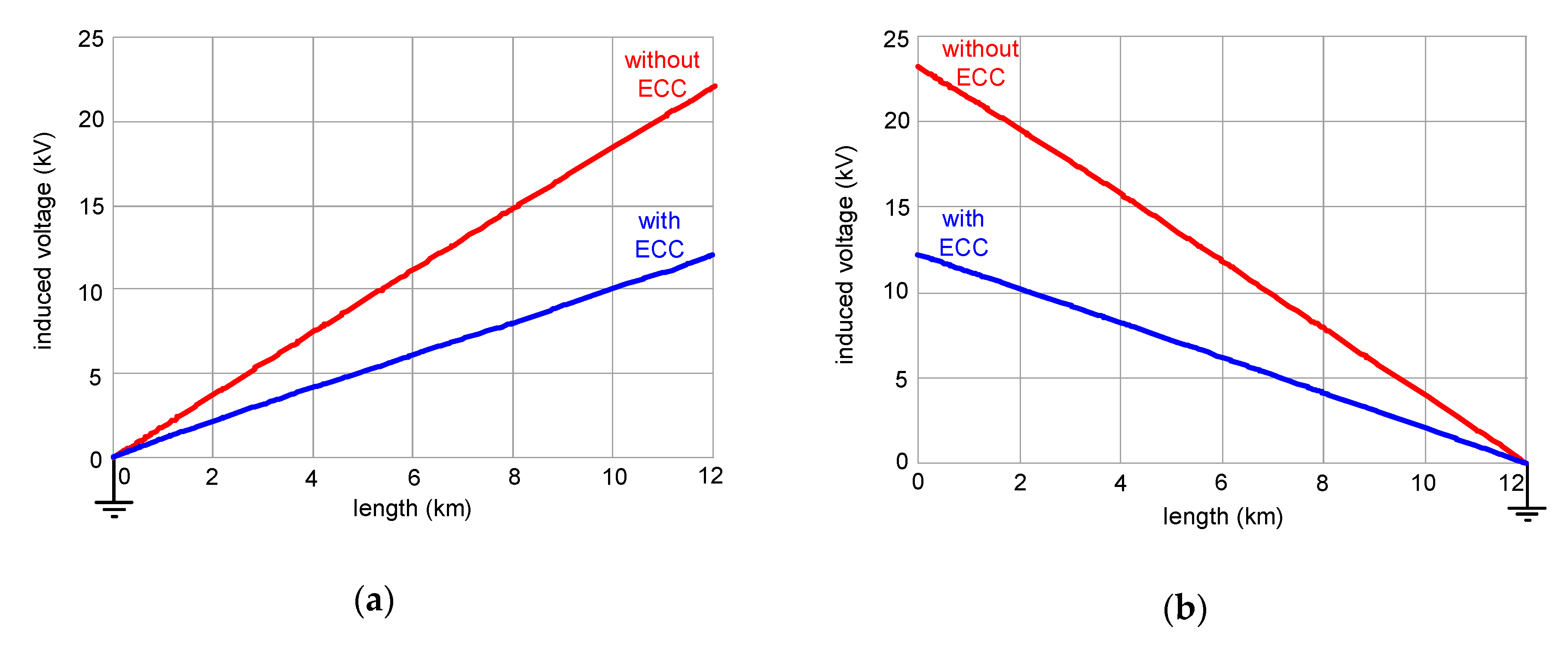
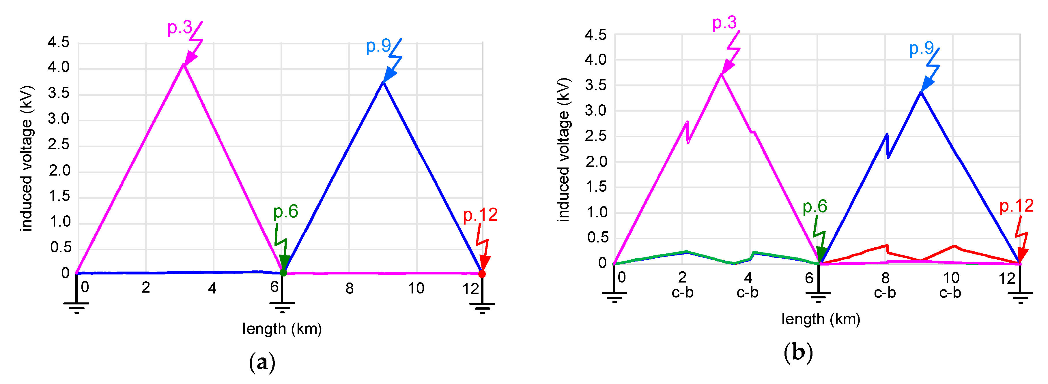
The next step of the analysis is to evaluate the induced sheath voltages in case of the line-to-earth fault at the unearthed end. Like in the previous scenarios, the single-point bonding was assumed alternatively at the 110 kV supply service substation (Figure 7a) or at the consumer substation (Figure 7b). In the short-circuit analysis, the induced voltages have been calculated for the cases without an earth continuity conductor (ECC) or with this conductor. The ECC was laid parallel to the cable line at a distance of 20 cm (Figure 8a). An insulated cable with a copper conductor of the cross-sectional area of 120 mm2 was assumed as the ECC. Halfway along the cable line (in p.6), the ECC was transposed to the other side of the line (Figure 8b), according to the recommendations included in the guide [2].
Induced sheath voltages at the unearthed end of the line reach values over 22 kV without the ECC and approx. 12 kV with the ECC. All respective values are similar, regardless, the single-point bonding and earthing are performed in p.0 or in p.12. Such high values of the induced voltages between the copper sheath and the earth may be a source of the damage of the non-metallic outer sheath of the cable (PE outer sheath in Figure 3). It is a common design practice to assume that this non-metallic outer sheath will not be damaged if the induced voltage does not exceed 5 kV. As it is seen in Figure 7, the value 5 kV is not exceeded only for the length of the cable line (from the earthing point) approx. 2.5 km without the ECC and approx. 5 km with the ECC. Thus, in the considered power line of the length 12 km, the single-point bonding is not acceptable—too high values of the induced voltages in case of the short-circuit conditions exist (despite the possible application of sheath voltage limiters (SVL); a high-level margin of reliability and safety is required).
3.2. Induced Voltages for Both-Ends Bonding or Cross Bonding
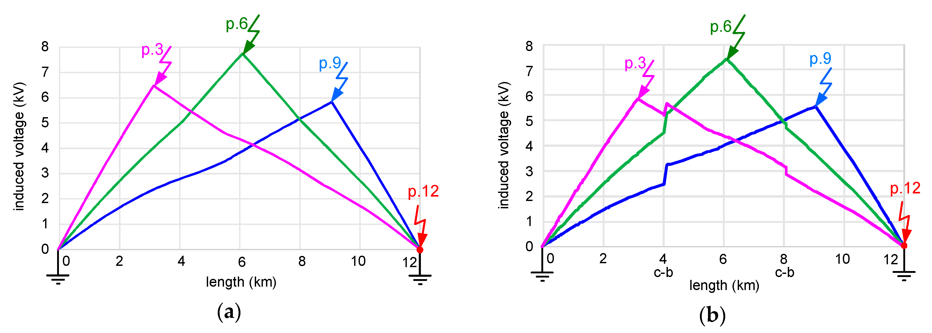
Since single-point bonding in the analyzed cable line is not acceptable, both-ends bonding is considered as an alternative solution. For the both-ends bonding, the induced sheath voltages in the normal operating conditions (10 MW) are close to 0 V. Therefore, they are not presented in the form of the chart in this paper. However, the induced voltages distributions are very interesting in case of the line-to-earth fault. The cable line comprises straight-joints approx. every 1 km. After discussion with the industrial partner involved in the cable line project, it was decided to analyze the induced voltages distribution in case of the earth fault in the selected joints. The line-to-earth fault was consecutively assumed in the following points (Figure 9):
- p.3: a quarter of the line length;
- p.6: half of the line length;
- p.9: three-quarters of the line length;
- p.12: the consumer substation.
The distributions of the induced voltages for the aforementioned points of the fault are presented in Figure 10. For the both-ends bonding (Figure 10a) the line-to-earth-fault at point p.12 gives induced voltage practically equal to 0 V. It is obvious because this point is located at the consumer substation, which contains an earthing system. An earth fault in points p.3, p.6 or p.9 gives the induced voltages higher than the assumed permissible limit 5 kV (at the point of the fault). The highest value of the voltage is in p.6 (over 7 kV) mainly because it is located at the farthest distance from the earthed points (p.0 and p.12). In the case of the cross bonding (transpositions of the cable sheaths are performed in p.4 and p.8; see Figure 10b), the induced voltages in the characteristic points are only slightly lower compared to the both-ends bonding. Unfortunately, the voltages still exceed the assumed permissible level of 5 kV.
To decrease the induced voltages below the permissible 5 kV, an additional earthing in point p.6 has been proposed. The earthing is relatively easy to perform in this place—the cables’ metallic sheaths are accessible. With this additional earthing, the power cable system is composed of three earthing points (p.0, p.6 and p.12) and the induced voltages distributions are as in Figure 11. As it was expected, in the case of the line-to earth fault in p.6, for the both-ends bonding (Figure 11a), the induced voltage in this point is reduced practically to 0 V. However, one can see that for the arrangement with the cross bonding (Figure 11b), in the case of the line-to earth fault in p.6, the induced voltage between p.0 and p.6 reaches approx. 250 V. Similar voltage distribution is observed between p.6 and p.12, in the case of the line-to earth in p.12. For both arrangements (both-ends bonding and cross bonding), the highest value of the voltage is around 4 kV (line-to-earth in p.3), what is clearly below the permissible value (5 kV).
Thus, the additional earthing in p.6 eliminates in a simple way the problem of too high induced sheath voltages in case of the short-circuit conditions. The both-ends bonding, as well as the cross bonding, can be employed (with additional earthing in p.6) but the latter is a more complicated solution.
4. Power Losses for the Analyzed Types of Bonding
During the selection of the type of bonding, which is to be used in a high-voltage cable system, an analysis of the power losses in this system is recommended to be performed. In the total power losses in the cable system, additional losses produced in the cable sheaths should be included. Generally, power losses ΔP3sh generated in three cables’ sheaths and power losses ΔP3c generated in three cables’ conductors (cores) can be calculated according to the following expressions:
where: ΔP3sh represents the power losses in three cables’ sheaths; ΔP3c represents the power losses in three cables’ conductors (cores); Ish-L1, Ish-L2, Ish-L3 are the currents flowing through the sheath of the cable in phases L1, L2 and L3, respectively; IL1, IL2, IL3 are the currents flowing through the conductor (core) of the cable in phases L1, L2 and L3, respectively; Rsh is the resistance of the cable’s sheath; Rc is the resistance of the cable’s conductor (core).
One of the main problems in the power losses calculation is to evaluate the real current distribution in each cable sheath (currents Ish-L1, Ish-L2, Ish-L3). It is relatively difficult to calculate analytically, especially when the arrangement of the cable line is varied or the cross bonding is applied. In this investigation, all the parameters have been calculated on the base of the data obtained from the PowerFactory software, taking into account the arrangement of the cables in every of 161 sections of the cable line.
Power losses in the cables’ sheaths can be very high in the case of both-ends bonding. Relatively high circulating currents may give a significant heat flux generation across the sheath’s resistance, which increases the temperature of the cables. However, in the power cable line under consideration, the contracted transferred power is relatively low compared to the transmission capacity of the line, so the selection of the type of the bonding system, from the point of view of the power losses, is not obvious.
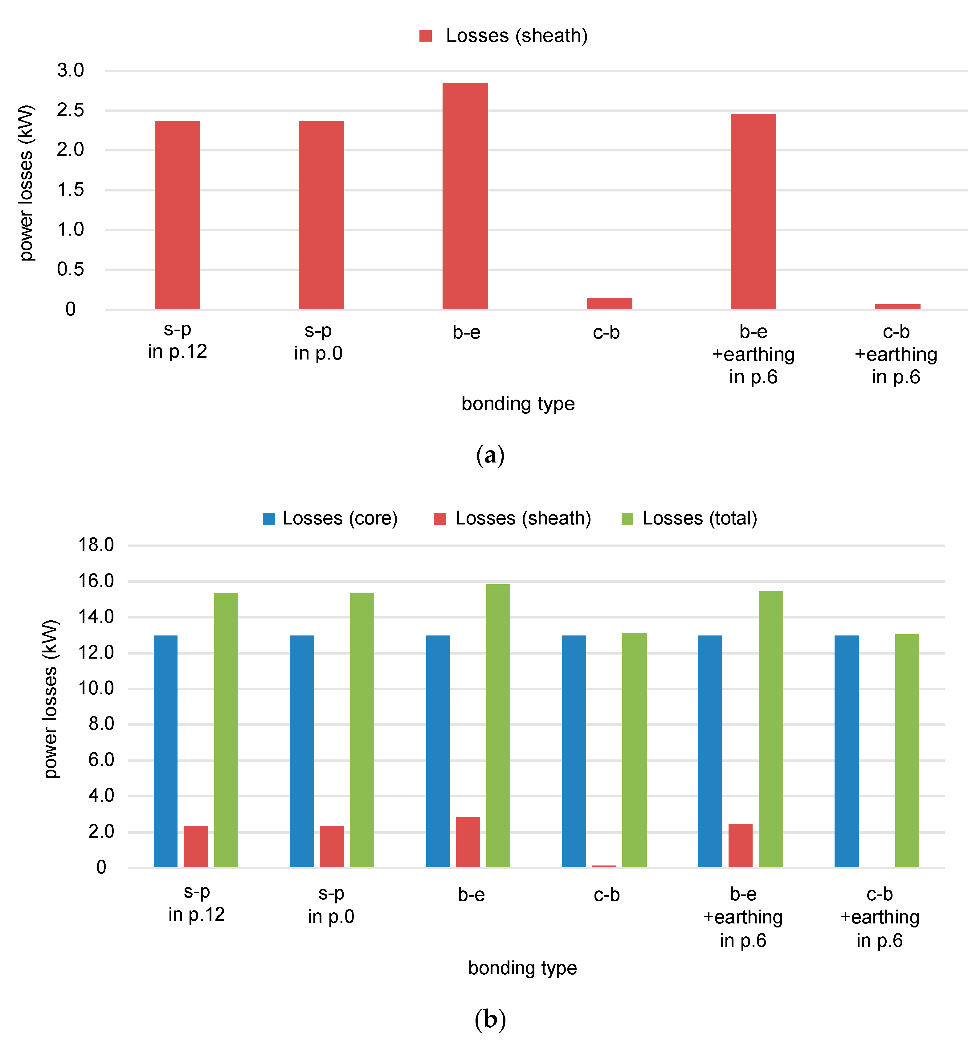
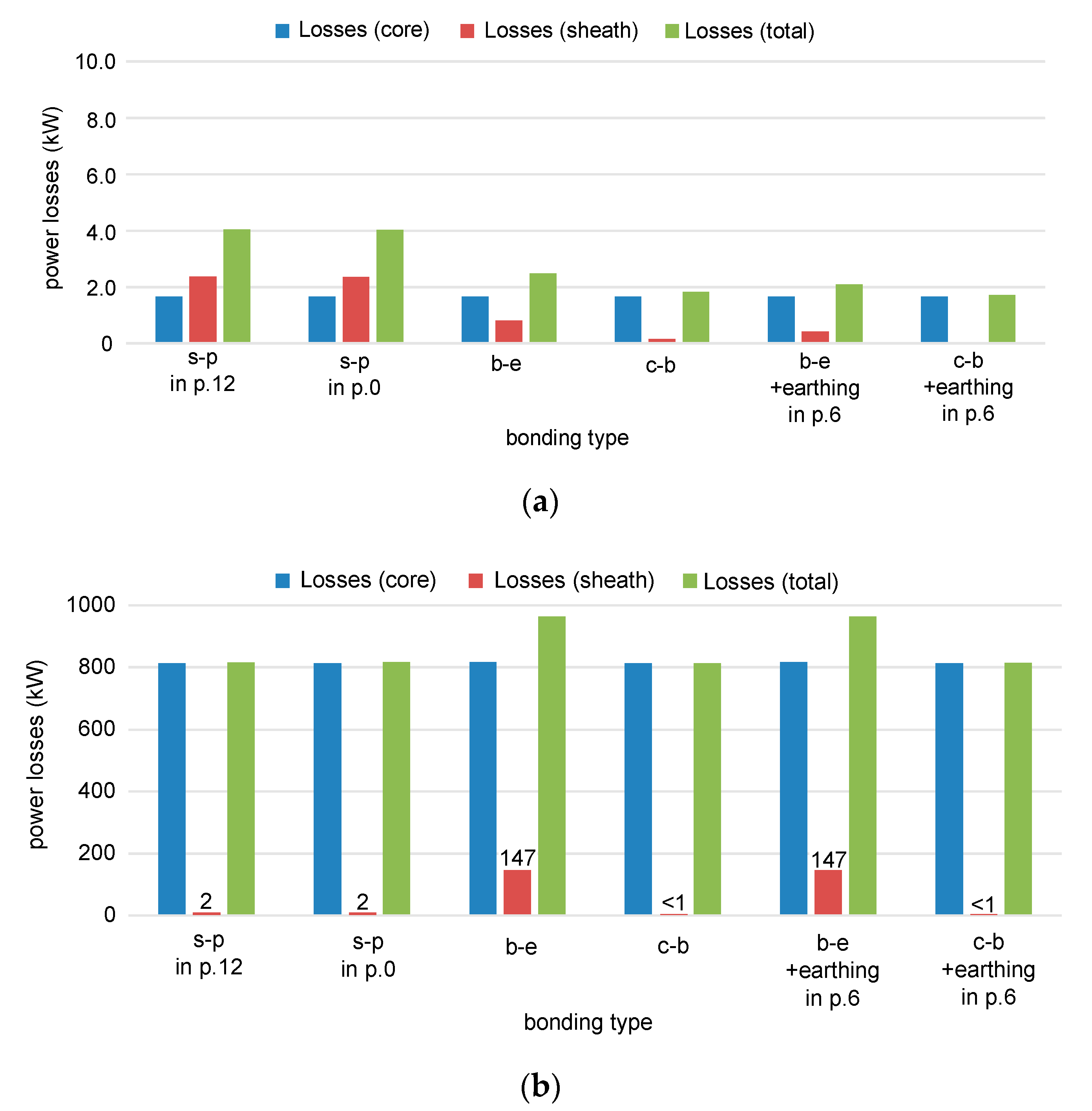
The power losses have been evaluated with the use of the aforementioned computer model of the cable system. Figure 12a presents power losses in the cable sheaths (all three phases) for the contracted transferred power (10 MW, tgϕ = 0.4) and the cable system arrangements, which are to be implemented in practice. The both-ends bonding gives, in fact, the highest value of the power losses, but it is only slightly higher than for the single-point bonding. Generally, for these two aforementioned types of bonding, the power losses are on the low and acceptable level. This is not a typical phenomenon. The almost equal power losses for these two arrangements are the effect of the natural capacitive power of the line. Since the consumer load (active power) in the cable line is at the low level, the natural power forces a reactive (capacitive) current circulation in the system, which gives observable losses. When the cross bonding is used, power losses in the copper sheaths are negligible, due to the compensation of the induced voltages in the consecutive minor sections. The comparison of all the analyzed types of losses (in cores, in sheaths, total; for 10 MW, tgϕ = 0.4) is presented in Figure 12b. The total power losses (in copper sheaths + aluminium cores) are almost the same, both for the single-point bonding and both-ends bonding. They are within the range 15.4–15.8 kW, whereas for the cross bonding they are at the level of 13 kW. Power losses in the cores are the same for every type of bonding.
The effect of the natural reactive power of the cable line is seen especially in Figure 13a when the transferred power is only 1 MW, tgϕ = 0 (for the simplicity of the analysis, only the active power transfer is modelled). The natural reactive power of the analyzed line of the length 12 km is approx. 6 Mvar and significantly exceeds the transferred active power (1 MW). In such low-load conditions (active load current in the cable core is approx. 5 A; reactive/capacitive current in the cable core is approx. 30 A), the single-point bonding gives the highest total power losses. It should also be noted that the reactive/capacitive current coming from the natural power of the line is not the same along its whole length—it is a normal phenomenon of the current flowing via capacitance-to-earth of the cables.
If the cable line transfers the power equal to 80 MW, tgϕ = 0 (Figure 13b), giving practically the max permissible load (load current approx. 420 A), the value of the power losses is two orders higher, compared to the results from Figure 13a. What was expected, the highest value of the power losses is for the both-ends bonding. In this case, when the transferred power is many times higher than the natural reactive power, the effect of the latter power is negligible.
The analysis of the results of the power losses calculations shows that all types of bonding are acceptable for the transferred power equal to 10 MW. Admittedly, the cross bonding gives the lowest losses but introduces the most complicated technical solution to the power line.
5. Conclusions
Most of the high-voltage power cable lines are significantly loaded in practice, so in normal operating conditions the induced sheath voltages or power losses may be high. In order to exclude the risk of the electric shock and the negative effect of the power losses in the long cable lines, during such load conditions, cross bonding of the cable sheaths is most often indicated as the best solution.
However, if the cable line carries a relatively low load, as in the analyzed case, the choice of the best type of the bonding system is not obvious. For the analyzed cable line, a comparison of the possible bonding and earthing solutions is presented in Table 1.
When the risk of electric shock in normal operating conditions is considered, the values of the induced sheath voltages are acceptable in every case—for single point-bonding the highest value is below the permissible 80 V and for both-ends bonding or cross bonding the voltages are close to 0 V.
In case of the line-to-earth fault, the single point-bonding is excluded in this cable line, due to very high induced voltages. For the system without ECC, the voltage reaches 22 kV. When the ECC is installed, it decreases only to 12 kV. In the light of the assumed permissible level being equal to 5 kV, these high-value voltages are dangerous for the outer non-metallic sheath of the cable. It should also be noted that, due to the induced voltages in the case of the earth fault, the both-ends bonding, as well as the cross bonding, requires an additional earthing in the middle of the power cable length (point p.6). Without this additional earthing, the voltages may exceed 7 kV but with the earthing, they are reduced to approx. 4 kV.
A comparison of the power losses shows that the best solution is the cross bonding but two other solutions are acceptable as well—the total losses in the cable system are within the range 15.4–15.8 kW for the single-point bonding and both-ends bonding, whereas for the cross bonding they are equal to 13 kW. Such low and comparable power losses are the effect of the relatively low transferred power (10 MW).
Considering the economic aspect and simplicity of the solution, the single-point bonding without ECC (no additional parallel cable is installed) or both-ends bonding (no equipment for transpositions of the sheaths is required) are recommended.
Taking into account all the aforementioned aspects, the both-end bonding or cross bonding can be used in the analyzed cable line. For each of the two solutions, the additional earthing in p.6 is required. To achieve safe operation of relatively long high-voltage cable lines, which are loaded in a low percentage, special attention must be given to the study of short-circuit currents. The induced sheath voltages coming from high-value currents can give unacceptably high-voltage stress, not only in the case of single-point bonding, but also in the case of both-ends bonding. In the latter case, this stress applies to points located close to the centre of the cable section between the earthing arrangements. In such a cable system, shorter distances between the earthing arrangements should be used.
Author Contributions
Conceptualization, S.C.; software, K.D.; validation, S.C. and K.D.; formal analysis, S.C.; investigation, S.C. and K.D.; resources, S.C.; writing—original draft preparation, S.C. and K.D.; writing—review and editing, S.C.; supervision, S.C. All authors have read and agreed to the published version of the manuscript.
Funding
This research was supported by Gdańsk University of Technology.
Conflicts of Interest
The authors declare no conflict of interest.
References
- Jaworski, M. Safety of staying and running field crops under overhead power lines. Prz. Elektrotechniczny 2019, 95, 17–21. [Google Scholar]
- IEEE. 575-2014 IEEE Guide for Bonding Shields and Sheaths of Single-Conductor Power Cables Rated 5 kV through 500 kV; Institute of Electrical and Electronics Engineers: Piscataway, NJ, USA, 2014. [Google Scholar]
- IEEE. 80-2013/Cor 1-2015 IEEE Guide for Safety in AC Substation Grounding; Institute of Electrical and Electronics Engineers: Piscataway, NJ, USA, 2015. [Google Scholar]
- CIGRE. Special Bonding of High Voltage Power Cables; Working group B1.18, Report Oct; CIGRE: Paris, France, 2005. [Google Scholar]
- Yi, Z.; Cao, X.; Wu, G.; He, F.; Zhang, X. Analysis of the sheath voltage in high-speed railway feeder cable grounding in single-ended mode. In Proceedings of the 2014 International Conference on Lightning Protection (ICLP), Shanghai, China, 11–18 October 2014. [Google Scholar]
- Akbal, B. Determination of the sheath current of high voltage underground cable line by using statistical methods. Int. J. Eng. Sci. Comput. 2016, 6, 2188–2192. [Google Scholar]
- Czapp, S.; Dobrzynski, K.; Klucznik, J.; Lubosny, Z. Computer-aided analysis of induced sheath voltages in high voltage power cable system. In Proceedings of the 10th International Conference on Digital Technologies, Zilina, Slovakia, 9–11 July 2014. [Google Scholar]
- Santos, M.; Calafat, M.A. Dynamic simulation of induced voltages in high voltage cable sheaths: Steady state approach. Int. J. Elect. Power Energy Syst. 2019, 105, 1–16. [Google Scholar] [CrossRef]
- Shaban, M.; Salam, M.A.; Ang, S.P.; Sidik, M.A.B. Assessing induced sheath voltage in multi-circuit cables: Revising the methodology. In Proceedings of the 2015 IEEE Conference on Energy Conversion (CENCON), Johor Bahru, Malaysia, 19–20 October 2015. [Google Scholar]
- CENELEC. EN 50522:2010. Earthing of Power Installations Exceeding 1 kV a.c.; European Committee for Electrotechnical Standardization: Brussels, Belgium, 2010. [Google Scholar]
- Czapp, S.; Dobrzynski, K.; Klucznik, J.; Lubosny, Z. Impact of configuration of earth continuity conductor on induced sheath voltages in power cables. In Proceedings of the 2016 International Conference on Information and Digital Technologies (IDT), Rzeszow, Poland, 5–7 July 2016; pp. 59–63. [Google Scholar]
- Lee, B.; Jung, C.K. Technical review on parallel ground continuity conductor of underground cable systems. J. Int. Council Elect. Eng. 2012, 2, 250–256. [Google Scholar]
- Parol, M.; Wasilewski, J.; Jakubowski, J. Assessment of electric shock hazard coming from earth continuity conductors in 110 kV cable lines. IEEE Trans. Power Deliv. 2020, 35, 600–608. [Google Scholar] [CrossRef]
- Colella, P.; Napoli, R.; Pons, E.; Tommasini, R.; Barresi, A.; Cafaro, G.; De Simone, A.; Di Silvestre, M.L.; Martirano, L.; Montegiglio, P.; et al. Currents distribution during a fault in an MV network: Methods and measurements. IEEE Trans. Ind. Appl. 2016, 52, 4585–4593. [Google Scholar] [CrossRef]
- Di Silvestre, M.L.; Dusonchet, L.; Salvatore, F.; Mangione, S.; Mineo, L.; Mitolo, M.; Riva Sanseverino, E.; Zizzo, G. On the interconnections of HV–MV stations to global grounding systems. IEEE Trans. Ind. Appl. 2019, 55, 1126–1134. [Google Scholar] [CrossRef]
- Asif, M.; Lee, H.-Y.; Park, K.-H.; Lee, B.-W. Accurate evaluation of steady-state sheath voltage and current in HVDC cable using electromagnetic transient simulation. Energies 2019, 12, 4161. [Google Scholar]
- Akbal, B. Hybrid GSA-ANN methods to forecast sheath current of high voltage underground cable lines. J. Comput. 2018, 13, 417–425. [Google Scholar] [CrossRef]
- Riba Riuz, J.R.; Garcia, A.; Morera, X.A. Circulating sheath currents in flat formation underground power lines. Renew. Energy Power Qual. J. 2007, 1, 61–65. [Google Scholar] [CrossRef]
- Gouda, O.; Faraq, A.A. Factors affecting the sheath losses in single-core underground power cables with two-points bonding method. Int. J. Electr. Comput. Eng. 2012, 2, 7–16. [Google Scholar] [CrossRef]
- Li, Z.; Du, B.X.; Wang, L.; Yang, C.; Liu, H.J. The calculation of circulating current for the single-core cables in smart grid. In Proceedings of the IEEE PES Innovative Smart Grid Technologies Asia, Tianjin, China, 21–24 May 2012. [Google Scholar]
- Zong, H.; Gao, Q.; Wang, R.; Wang, H.; Liu, Y. Calculation and restraining method for circulating current of single core high voltage cable. In Proceedings of the 2nd International Conference on Electrical Materials and Power Equipment (ICEMPE), Guangzhou, China, 7–10 April 2019. [Google Scholar]
- Liang, W.; Zhou, Z.; Pan, W.; Li, Y.; Zhou, Q.; Zhu, M. Study on the calculation and suppression method of metal sheath circulating current of three-phase single-core cable. In Proceedings of the IEEE PES Asia-Pacific Power and Energy Engineering Conference (APPEEC), Macao, Macao, 1–4 December 2019. [Google Scholar]
- Jung, C.K.; Lee, J.B.; Kang, J.W.; Wang, X.; Song, Y.-H. Characteristics and reduction of sheath circulating currents in underground power cable systems. Int. J. Emerg. Electr. Power Syst. 2004, 1. [Google Scholar] [CrossRef]
- Ariyasinghe, A.; Warnakulasuriya, C.; Kumara, S.; Fernando, M. Optimizing medium voltage underground distribution network with minimized sheath and armor losses. In Proceedings of the 2019 14th Conference on Industrial and Information Systems (ICIIS), Kandy, Sri Lanka, 18–20 December 2019. [Google Scholar]
- Sobral, A.; Moura, A.; Carvalho, M. Technical implementation of cross bonding on underground high voltage lines projects. In Proceedings of the 21st International Conference on Electricity Distribution, Frankfurt, Germany, 6–9 June 2011. [Google Scholar]
- Noufal, S.; Anders, G. Sheath loss factor for cross-bonded cable systems with unknown minor section lengths field verification of the IEC standard. IEEE Trans. Power Deliv. 2020. [Google Scholar] [CrossRef]
- Jung, C.K.; Lee, J.B.; Kang, J.W.; Wang, X. Sheath circulating current analysis of a crossbonded power cable systems. J. Electr. Eng. Technol. 2007, 2, 320–328. [Google Scholar] [CrossRef] [Green Version]
- Li, M.; Zhou, C.; Zhou, W.; Wang, C.; Yao, L.; Su, M.; Huang, X. A novel fault location method for a cross-bonded HV cable system based on sheath current monitoring. Sensors 2018, 18, 3356. [Google Scholar] [CrossRef] [PubMed] [Green Version]
- Li, M.; Zhou, C.; Zhou, W. A revised model for calculating HV cable sheath current under short-circuit fault condition and its application for fault location—Part 1: The revised model. IEEE Trans. Power Del. 2019, 34, 1674–1683. [Google Scholar] [CrossRef]
- Weissenberg, W.; Farid, F.; Plath, R.; Rethmeier, K.; Kalkner, W. On-site PD detection at cross-bonding links of HV cables, CIGRE, Group B1: Insulated Cables. In Cigre Session 2004; CIGRE: Paris, France, 2004. [Google Scholar]
- Power Cable XRUHAKXS 1x240/95 mm2, 64/110 kV. In Technical Specification (In Polish); TELE-FONIKA Kable: Krakow, Poland, 2017.
- PowerFactory: Integrated Power System Analysis Software; DIgSILENT GmbH: Gomaringen, Germany, 2018.
- Ametani, A. A general formulation of impedance and admittance of cables. IEEE Trans. Power Appar. Syst. 1980, PAS-99, 902–910. [Google Scholar] [CrossRef]
- DIgSILENT PowerFactory. Technical Reference Documentation, Cable System; DIgSILENT GmbH: Gomaringen, Germany, 2014. [Google Scholar]
Figure 1.
High-voltage power cables arrangements: (a) single-point bonding; (b) both-ends bonding; (c) cross bonding.
Figure 1.
High-voltage power cables arrangements: (a) single-point bonding; (b) both-ends bonding; (c) cross bonding.

Figure 2.
General data of the analyzed power cable system; p.0–p.12—possible points for earthing and bonding.
Figure 2.
General data of the analyzed power cable system; p.0–p.12—possible points for earthing and bonding.

Figure 3.
A simplified view of the power cable used in the analyzed case.

Figure 4.
Real cable route of the analyzed cable system reflected in the PowerFactory software (a); an example part of the computer model of the cable system (minor section between point p.0 and point p.1) (b).
Figure 4.
Real cable route of the analyzed cable system reflected in the PowerFactory software (a); an example part of the computer model of the cable system (minor section between point p.0 and point p.1) (b).

Figure 5.
Induced sheath voltages as a function of the cable line length, for three values of the transferred power (1 MW, 10 MW, 80 MW), tgϕ = 0: (a) single-point bonding at point p.0 in Figure 2; (b) single-point bonding at point p.12 in Figure 2.

Figure 6.
Induced sheath voltages as a function of the cable line length for three values of the transferred power (1 MW, 10 MW, 80 MW), tgϕ = 0.4: (a) single-point bonding at point p.0 in Figure 2; (b) single-point bonding at point p.12 in Figure 2.

Figure 7.
Induced sheath voltages as a function of the cable line length, in case of the line-to-earth fault at the unearthed end; single-point bonding at: (a) supply service substation (point p.0 in Figure 2); (b) consumer substation (point p.12 in Figure 2).

Figure 8.
Arrangement of the earth continuity conductor (ECC): (a) a distance to the cable line; (b) its transposition.
Figure 8.
Arrangement of the earth continuity conductor (ECC): (a) a distance to the cable line; (b) its transposition.

Figure 9.
Simplified diagram of the cable system presenting points of the assumed consecutive line-to-earth faults.
Figure 9.
Simplified diagram of the cable system presenting points of the assumed consecutive line-to-earth faults.

Figure 10.
Induced sheath voltages as a function of the cable line length, in case of the line-to-earth fault in the characteristic points (p.3, p.6, p.9 or p.12): (a) both-ends bonding; (b) cross bonding (c-b) in p.4 and p.8.
Figure 10.
Induced sheath voltages as a function of the cable line length, in case of the line-to-earth fault in the characteristic points (p.3, p.6, p.9 or p.12): (a) both-ends bonding; (b) cross bonding (c-b) in p.4 and p.8.

Figure 11.
Induced sheath voltages as a function of the cable line length, in case of the line-to-earth fault in characteristic points (p.3, p.6, p.9 or p.12); additional earthing in p.6: (a) both-ends bonding; (b) cross bonding (c-b) in p.2, p.4 as well as in p.8, p.10.
Figure 11.
Induced sheath voltages as a function of the cable line length, in case of the line-to-earth fault in characteristic points (p.3, p.6, p.9 or p.12); additional earthing in p.6: (a) both-ends bonding; (b) cross bonding (c-b) in p.2, p.4 as well as in p.8, p.10.

Figure 12.
Power losses in the analyzed three-phase cable system for the transferred power 10 MW, tgϕ = 0.4: (a) losses in the metallic sheaths; (b) comparison of the losses in the metallic sheaths, cores and total losses; s-p: single-point bonding; b-e: both-ends bonding; c-b: cross bonding.
Figure 12.
Power losses in the analyzed three-phase cable system for the transferred power 10 MW, tgϕ = 0.4: (a) losses in the metallic sheaths; (b) comparison of the losses in the metallic sheaths, cores and total losses; s-p: single-point bonding; b-e: both-ends bonding; c-b: cross bonding.

Figure 13.
Power losses in the analyzed three-phase cable system: (a) for the transferred power 1 MW, tgϕ = 0; (b) for the transferred power 80 MW, tgϕ = 0; s-p: single-point bonding; b-e: both-ends bonding; c-b: cross bonding.
Figure 13.
Power losses in the analyzed three-phase cable system: (a) for the transferred power 1 MW, tgϕ = 0; (b) for the transferred power 80 MW, tgϕ = 0; s-p: single-point bonding; b-e: both-ends bonding; c-b: cross bonding.


Table 1.
A summary of the properties of the bonding systems in the analyzed cable line.
| Criterion | Single-Point Bonding | Both-Ends Bonding | Cross Bonding |
|---|---|---|---|
| Induced voltages in normal operating condition | (0) 1 | (0) | (0) |
| Induced voltages in the case of the short circuit | (-) | (+) with earthing in p.6 | (+) with earthing in p.6 |
| Power losses in the cable system | (0) | (0) | (+) |
| Simplicity of the solution and economic aspects | (+) (0) with ECC | (+) | (0) |
1 Markings: (+) preferred solution; (0) acceptable solution; (-) excluded solution.
© 2020 by the authors. Licensee MDPI, Basel, Switzerland. This article is an open access article distributed under the terms and conditions of the Creative Commons Attribution (CC BY) license (http://creativecommons.org/licenses/by/4.0/).
Share and Cite
MDPI and ACS Style
Czapp, S.; Dobrzynski, K. Safety Issues Referred to Induced Sheath Voltages in High-Voltage Power Cables—Case Study. Appl. Sci. 2020, 10, 6706. https://doi.org/10.3390/app10196706
AMA Style
Czapp S, Dobrzynski K. Safety Issues Referred to Induced Sheath Voltages in High-Voltage Power Cables—Case Study. Applied Sciences. 2020; 10(19):6706. https://doi.org/10.3390/app10196706
Chicago/Turabian StyleCzapp, Stanislaw, and Krzysztof Dobrzynski. 2020. "Safety Issues Referred to Induced Sheath Voltages in High-Voltage Power Cables—Case Study" Applied Sciences 10, no. 19: 6706. https://doi.org/10.3390/app10196706
Note that from the first issue of 2016, this journal uses article numbers instead of page numbers. See further details here.