Dynamic Analysis of Cavitation Tip Vortex of Pump-Jet Propeller Based on DES
by
Jianping Yuan
1,2, 
Yang Chen
1,2,
Longyan Wang
1,3,*,
Yanxia Fu
1,4,*,
Yunkai Zhou
1,2,
Jian Xu
1,2 and
Rong Lu
1,2 1
National Research Center of Pumps, Jiangsu University, Zhenjiang 212013, China
2
Institute of Fluid Engineering Equipment, JITRI, Jiangsu University, Zhenjiang 212013, China
3
School of Chemistry, Physics and Mechanical Engineering, Queensland University of Technology, Brisbane 4001, Australia
4
School of Energy and Power Engineering, Jiangsu University, Zhenjiang 212013, China
*
Authors to whom correspondence should be addressed.
Appl. Sci. 2020, 10(17), 5998; https://doi.org/10.3390/app10175998
Submission received: 31 July 2020
/
Revised: 21 August 2020
/
Accepted: 24 August 2020
/
Published: 29 August 2020
(This article belongs to the Section Marine Science and Engineering)
Abstract
:When a pump-jet propeller rotates at high speeds, a tip vortex is usually generated in the tip clearance region. This vortex interacts with the main channel fluid flow leading to the main energy loss of the rotor system. Moreover, operating at a high rotational speed can cause cavitation near the blades which may jeopardize the propulsion efficiency and induce noise. In order to effectively improve the propulsion efficiency of the pump-jet propeller, it is mandatory to research more about the energy loss mechanism in the tip clearance area. Due to the complex turbulence characteristics of the blade tip vortex, the widely used Reynolds averaged Navier–Stokes (RANS) method may not be able to accurately predict the multi-scale turbulent flow in the tip clearance. In this paper, an unsteady numerical simulation was conducted on the three-dimensional full flow field of a pump-jet propeller based on the DES (detached-eddy-simulation) turbulence model and the Z-G-B (Zwart–Gerber–Belamri) cavitation model. The simulation yielded the vortex shape and dynamic characteristics of the vortex core and the surrounding flow field in the tip clearance area. After cavitation occurred, the influence of cavitation bubbles on tip vortices was also studied. The results revealed two kinds of vortices in the tip clearance area, namely tip leakage vortex (TLV) and tip separation vortex (TSV). Slight cavitation at J = 1.02 led to low-frequency and high-frequency pulsation in the TLV vortex core. This occurrence of cavitation promotes the expansion and contraction of the tip vortex. Further, when the advance ratio changes into J = 0.73, a third type of vortex located between TLV and TSV appeared at the trailing edge which runs through the entire rotational cycle. This study has presented the dynamic characteristics of tip vortex including the relationship between cavitation bubbles and TLV inside the pump-jet propeller, which may provide a reference for the optimal design of future pump-jet propellers.
1. Introduction
Since the 1980s, pump-jet propellers have gradually attracted the attention of military industries in various countries due to their advantages of high propulsion efficiency, low radiation noise, and extraordinary anti-cavitation performance [1,2]. In recent years, with the development of water transportation towards high speed, the application scope and demand of pump-jet propellers have been drastically increasing. As is well known, when the rotational speed of the pump rotor is increasingly high, the pressure in the high-speed region is the lowest which, as a result, means the cavitation is most likely to occur. In most instances, e.g., propellers and pumps, the cavitation is an undesirable phenomenon causing intensive noise, component damage, vibration and loss of efficiency [3,4]. The shock wave generated by the collapse of the bubble is the main source of noise, which particularly in the marine military field, poses a great threat to the art of stealth during underwater navigation. Above all, it is mandatory to study the cavitation characteristics of a pump-jet propeller for its wide applications.
Recently, as more and more scholars have paid attention to new underwater propeller systems, the research of pump-jet propeller has become more and more abundant. Because of expensive cost of test rig, there are still only a few experimental researches about the pump-jet performance. Suryanarayana et al. [5,6,7] studied the thrust and resistance of a pump-jet propeller. Through experiments in a cavitation water tunnel, it was found that at a higher inflow velocity coefficient, cavitation of the rotor first occurs at the blade tip and with the increase of the rotational speed, the cavitation bubbles shift to the suction side, while the stator and the duct do not exhibit cavitation. Shirazi et al. [8] conducted bollard pull, self-propulsion point, and bare hull resistance tests in a towing tank on a full scale pump-jet model to research hydraulic performance, and he found that the variations of hydraulic coefficients are much smaller than conventional propellers as the advance coefficient varies.
With the advantages of cost saving and more detailed flow field information, numerical simulation results are more plentiful than experiments researches. Das et al. [9] numerically analyzed the fluid flow of a high-speed underwater vehicle with a pump-jet propulsion system. Dong et al. [10] used Fluent software to numerically simulate the underwater vehicle equipped with pump-jet propulsion based on the RNG k-ε turbulence model, which provides an important reference for pump-jet thruster optimization. A numerical study on a pump-jet propeller equipped with a ring at the blade tip was conducted by Ahn and Kwon [11], the results showed that the addition of the ring could help reduce the tip vortex strength which may prevent the generation of tip leakage cavitation. Shi et al. [12] performed a steady analysis of the three-dimensional full-channel cavitation flow field of a pump-jet propeller based on the Rayleigh–Plesset equation and the k-ε turbulence model. Compared with the experimental test, it is found that, when cavitation occurs inside the pump-jet propeller, the open water efficiency can be reduced by more than 15%. Lin et al. [13] simulated the unsteady characteristics of a pump-jet propeller based on the shear stress transport (SST) k-ω turbulence model and the Z-G-B (Zwart–Gerber–Belamri) cavitation model. It was found that, among the rotor blade tip area, cavitation tip vortex will be formed due to the pressure difference between the pressure side and the suction side, which will cause local pressure to decrease, followed by the reduction of propulsion efficiency of the pump-jet. Pan et al. [14] conducted a numerical simulation of a pump-jet propeller based on the RANS (Reynolds averaged Navier–Stokes) solver and the SST k-ω turbulence model. They found that the presence of blade tip vortices would lead to a further reduction in propulsion efficiency which is likely to cause cavitation. Lu et al. [15] further studied the effect of tip clearance on pump cavitation performance. He pointed out that when the rotor tip clearance is large, the cavitation phenomenon is more obvious leading to a lower propulsion efficiency. However, it should also be noted that the size of the tip clearance cannot be too small, otherwise excessive viscous force in the tip area will hinder the flow of fluid which is unfavorable for the pump-jet propeller. Qin et al. [16] also conducted a numerical simulation that focused on the influence of tip clearance size on pump-jet propeller, and concluded that the core of tip leakage vortex and tip separation vortex are closer as the tip gap size increases. Li et al. [17] used the DES (detached-eddy-simulation) method to study the uniform cavitation flow field of a pump-jet propeller. It was found that when the cavitation occurs, the range of TLV (tip leakage vortex) will increase in the circumferential direction. Furthermore, the intensity of TLV in the downstream non-cavitation area will also increase, while the intensity of TSV (tip separation vortex) will decrease. Wang et al. [18] proposed a new tip vortex model based on the actual flow condition in the pump-jet, which made the pressure distribution in the tip clearance closer to the viscous flow results. Qiu et al. [19] analyzed the time domain curves and frequency domain curves and he found that the pulsation pressure is greater in the blade tip position.
Because of the accurate prediction of flow separation at the separated region than URANS (unsteady Reynolds-averaged Navier-Stokes) method, more and more scholars employed a detached eddy simulation (DES) turbulence model in their studies. DES is a hybrid of the RANS (Reynolds-averaged Navier–Stokes) model and LES (large eddy simulation) model in which the model switches to a subgrid scale formulation in regions fine enough for LES calculations. Gong et al. [20] used the DES method to simulate the blade tip vortex, hub vortex and secondary vortex in the duct propeller. Huang et al. [21] achieved the accurate simulation of the three-dimensional dynamic vortex structure inside a turbine by using the DES turbulence model, and it shows a good agreement with the qualitative analysis of the turbine working under deviation from design conditions. Dawi et al. [22,23,24] combined a finite volume method with IDDES (improved delayed detached eddy simulation) turbulence model to compute direct noise and compared with experimental results which showed good agreement. In the research of Sun et al. [25], numerical simulation based on DES revealed that the strength of the tip vortices has an important influence on the onset of the instability of propeller wake. Through numerical simulation which used DES turbulence model, Lungu [26] found a more aggressive vortex structure in the wake. In order to simulate the fluid flow accurately in a pump-jet propeller with a front-mounted stator, Li et al. [27] used the RANS and DES method to conduct the computation. It was found that DES can better simulate the turbulent characteristics than RANS solver. Compared with the RANS method, the RANS/LES hybrid method can capture a more detailed vortex structure, while the computing resources required are not as large as the LES. Hence, the hybrid model has now been adopted by more and more scholars.
Cavitation is a pretty complex phenomenon that is easily appeared in turbo machinery operated at a high rotational speed. In addition, cavitation bubbles interacting with tip vortex will be more complicated which may deteriorate the fluency of flow field. Compared with pump-jet propellers, the research findings of cavitation and tip vortex of other axial flow machines are more abundant. Li, G.-N. et al. [28] took the standard propeller DTMB-4119 as the test object, and analyzed the propeller wake field through the PIV test method. They found that there are positive and negative vortices in the propeller tail vortex, which are generated on the suction side and pressure side of the blade, respectively. Zhang et al. [29] simulated and tested the tip vortex of an axial pump at three different flow rates based on the SST k-ω turbulence model. The results indicate that, as the flow rate increases, the tip vortex gradually moves toward the pressure side of the adjacent blade, and the initial point of the tip vortex will also move from the leading edge to the midpoint of the chord. Focused on symmetrical tip clearance and unsymmetrical tip clearance, Hao et al. [30] applied an improved cavitation model on a mixed flow pump as turbine at pump mode and the results showed that unsymmetrical tip clearance has more influence on radial force than symmetrical tip clearance. Zhang et al. [31] simulated the tip leakage vortex cavitating flow based on improved SST k-ω turbulence model and Rayleigh–Plesset cavitation model combined with the test data provided by a high-speed imaging system. They revealed the vortex dynamics of TLV cavitation, tip corner vortex cavitation, shear layer cavitation, and blowing cavitation. Furthermore, the TLV cavitation patterns are also demonstrated which clearly explain the spatial evolution of TLV cavitating flow. Four types of transition model are analyzed and compared by Wen et al. [32], which make great contributions to transition research and modeling in the future.
In summary, though there have been studies on the internal vortex structure and cavitation performance of the pump-jet propeller, the correlation analysis of the interaction between cavitation and the vortex dynamics has been few, especially for the study of vortex core pressure of the pump-jet propellers. Therefore, this paper aims to fill the research gap. The main focus is to investigate the shape and dynamic characteristics of the TLV and TSV that appears in the rotor tip clearance area before and after cavitation under different rotational speeds by DES turbulent model. The vorticity transport equations are applied for the first time to research the effect of cavitation occurrence on the tip vortex evolution mechanism in pump-jet. Furthermore, the Q criterion is used to identify the vortex core before and after cavitation, respectively.
The numerical settings in this research are based on previous work [33,34,35,36,37,38,39]. For the purpose of verifying the accuracy and reliability of the numerical work in this study, two other researches focused on pump-jet thruster conducted with experiment have been referred. Shirazi et al. [8] obtained numerical and experimental thrust and torque coefficients curves at Bollard pull condition at different rotor spins, and the numerical results agreed well with experimental results. Suryanarayana et al. [7] could predict the cavitation inception point well compared with test data. Moreover, Yu et al. [40,41] simulated a post-rotor pump-jet propeller with the same turbulent model as this research and compared with test data acquired in a cavitation tunnel, the computational results have a good agreement with the experiment data. The difference between numerical results and experimental results is small, which indicates the feasibility of the numerical calculation.
In this paper, the structure arrangement is as follows. Numerical method and computational setup are described in Section 2, including pump-jet model and grid independence analysis. In Section 3, the vortex dynamics and the interaction between cavitation and vortex are analyzed, in addition, the pressure propulsion of tip separation vortex is compared between different working conditions. Finally, a summary of the results overview is exhibited in Section 4.
2. Numerical Method and Computational Setup
2.1. Governing Equation
In this study, the homogeneous mixed flow model is used for the numerical simulation. The continuity equation and momentum equation based on the homogeneous mixed flow model are as follows:
where ρm is the density of the mixture, which is equal to αvρv + (1 − αv)ρl, and ρl is the density of the liquid phase, ρv is the vapor phase density; αv is the volume fraction of the vapor phase, ui and uj are the velocity component in the i direction and the j direction, respectively, μm is the dynamic viscosity of the mixed phase which is equal to μl(1 − αv) + μvαv, and μt is turbulent viscosity.
2.2. Turbulence Model
In order to improve the predictive accuracy of turbulence models in highly separated areas, Spalart, P.R. [42] proposed a method which combines RANS and LES, i.e., DES (detached eddy simulation). Its basic idea is to use RANS to solve the computation in the boundary layer near the wall and LES method in the boundary layer separation area. In this manner, not only the low cost of RANS method to solve the boundary layer area computation can be retained, but also the accurate prediction in the separation area is achieved. As a result, a more exquisite flow field information can be obtained. The simulation in this study is performed using ANSYS CFX 17.2 [30] commercial software. Hence, the turbulence model is DES model based on SST k-ω and the governing equation is as follows:
where, in the equation, the expression of turbulent viscosity coefficient is expressed by:
in which, F1 and F2 are blending functions, S is the amplitude of curl, while a1, σω2, β*, β, σk, and σω are constants. The values of the above terms are: a1 = 0.31, β* = 0.09, σk1 = 2, σk2 = 1, σω1 = 2, σω2 = 1.1682.
Binding the function F1 and F2 is the key to the successful application of the turbulence model. The formula of the blending function can be obtained as:
where y is the nearest distance from the grid to the wall. When the y value is small, it tends to be the k-ω model, while when the y value is large, it tends to be the k-ε model. In the SST k-ω turbulence model, the diffusion term Yk caused by turbulence is generally represented by:
while in the DES turbulence model, it is changed to be:
where Cdes is the calibration constant, which is 0.61, and Δmax is the maximum edge length of the local computational cell.
2.3. Cavitation Model
The cavitation model is composed of a set of mathematical equations which describe the mass transfer rate between liquid phase and vapor phase. In previous studies, Yan et al. [43] used the SST k-ω turbulence model and Z-G-B cavitation model to research the cavitating turbulent flow near the rotor suction surface. Further, combining with the experiment method, the cavitation performance curve showed good agreement with test data. Sikirica et al. [44] can predict tip vortex cavitation and sheet cavitation near hub of propeller well based on commercial solver Fluent and STAR-CCM+, which is validated by experimental observation. Xu et al. [45] conducted a cavitating numerical simulation with Z-G-B cavitation for a water-jet pump, through comparing with experimental results, the predicted cavitation performance curves exhibits reasonable agreement with them. In addition, the time-dependent vapor iso-surfaces are in accordance with high-speed video at different times in a typical cycle. Therefore, given that pump-jet propeller has similar geometry with propeller and water-jet pump, this study will employ Z-G-B cavitation model to calculate the mass transfer rate between liquid phase and vapor phase.
This study employs the Zwart–Gerber–Belamri cavitation model in CFX 17.2 software, which assumes that all bubbles in a system have the same initial diameter. The mass change rate for a single bubble is expressed by:
The vapor volume fraction is calculated by:
where mB is the bubble mass, VB is the bubble volume, ρv is the vapor phase density, ρl is the liquid density, pv is the vaporization pressure of liquid at local temperature, p is the liquid pressure around the bubble, αv is the vapor volume fraction, NB is the bubble number per unit volume, and RB is the bubble radius.
The total interphase mass transfer rate is calculated as:
The cavitation collapse process can be described by the following equation:
where Re is vapor generation rate. The concrete expression of Zwart-Gerber-Belamri cavitation model can be obtained by replacing the αv term with αnuc(1-αv) as:
in which the vapor volume fraction αnuc = 5 × 10⁻⁴, the empirical correction factor for vaporization Fvap = 50, and the condensation empirical correction factor Fcond = 0.001.
2.4. Numerical Approach Validation
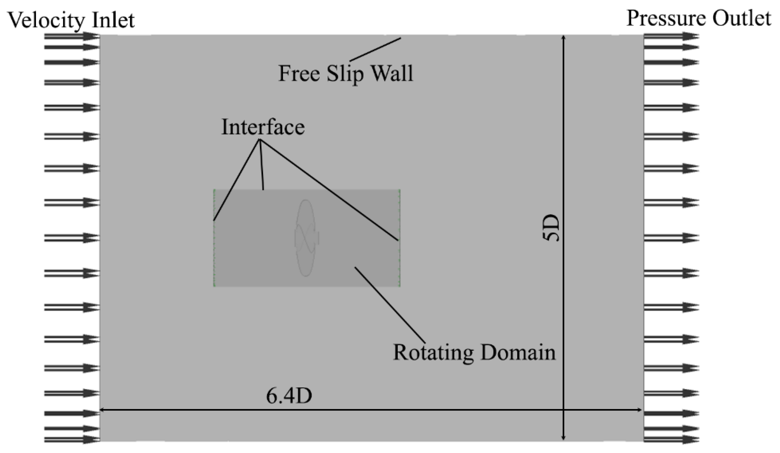
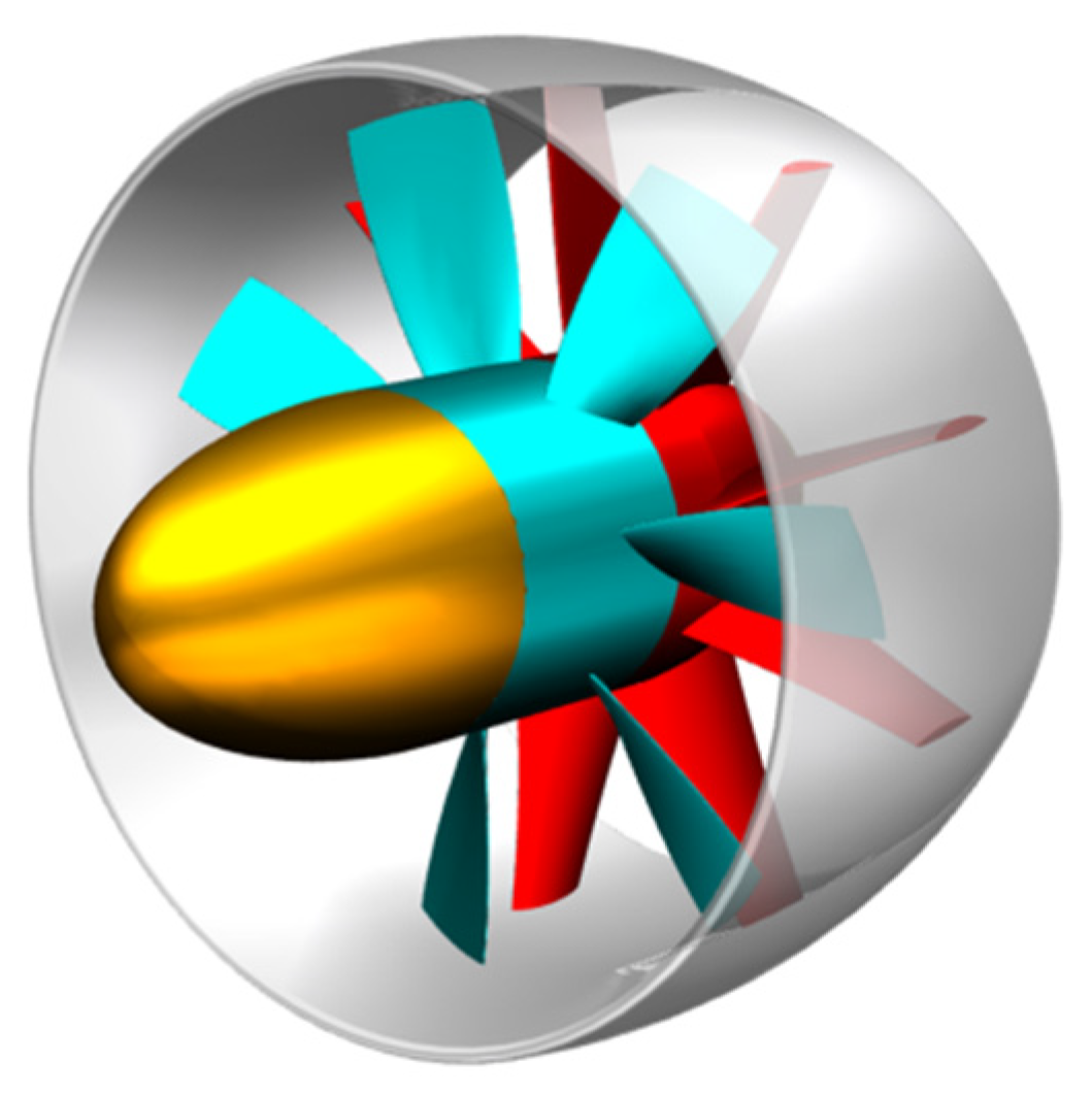
E779A is one of the most popular propellers used by many scholars because of its substantial experiment results [46,47,48]. Because cavitation experiments have been conducted in Italian Navy cavitation tunnel facility in 2006, in this paper, E779A propeller was selected to test the numerical simulated feasibility. The geometry and boundary conditions are shown as Figure 1, the outer cylindrical domain is external flow field and the inner one is rotational domain. The advance ratio is defined as J = U∞/(nD), where U∞ represents the oncoming flow velocity, while n and D are rotational speed and diameter of propeller, respectively. In order to compare with cavitation experiments data, outlet boundary was set into static pressure that varied according to cavitation number σ = (pout − pv)/(0.5*ρU∞2), where pout is outlet pressure, pv is saturation pressure under local temperature.
The SST k-ω turbulence model and Z-G-B cavitation model were used in the cavitation simulation of E779A propeller. Figure 2 shows the comparison between calculation and experiment results. In Figure 2, Kt is the thrust coefficient and Kq is the torque coefficient which are defined as Kt = T/(ρn2D4) and Kq = q/(ρn2D5), respectively, where T is the thrust and q is the torque of propeller. The propulsion efficiency η is defined as η = Kt/Kq*J/(2π). It can be seen from Figure 2 that numerical results agree well with the experimental data, which indicates that the numerical approach employed by this paper is reliable.
2.5. Three-Dimensional Model and Mesh
2.5.1. Three-Dimensional Model
The pump-jet propeller used in this paper is shown in Figure 3. The stator is rear-mounted, and the number of rotor blades and stator blades are 7 and 9 respectively. The minimum distance between the rotor blades and the wall is 1.37 mm, and the direction of rotation is counterclockwise (viewed from the back). The computational domain is divided into three parts: external flow field, rotor system and stator system, for which only the rotor system is the rotational domain while the others are the stationary domain. Therefore, for the steady computation, the interface between the rotor system and the external flow field and the interface between the rotor system and the stator system are set to be the frozen rotor in ANSYS CFX 17.2 software designed by Ansys, Inc in 2016 from Canonsburg, PA, USA.
2.5.2. Mesh and Boundary Conditions
In order to simulate the operation of the pump-jet propeller in a marine environment, the pump-jet propeller was placed in a large cylindrical area, i.e., the external flow field, with the same axis as the pump-jet propeller shown in Figure 4. The external flow field inlet was set as the speed inlet, and outlet was set as the static pressure outlet. The cylindrical wall was set as the free slip wall, while other walls were set as the non-slip wall. The maximum diameter of rotor of the pump-jet propeller is D. The inlet and outlet boundary of computational domain of the external flow field are 4D and 6D away from the rotor, respectively. The diameter of the external flow field is 5D.
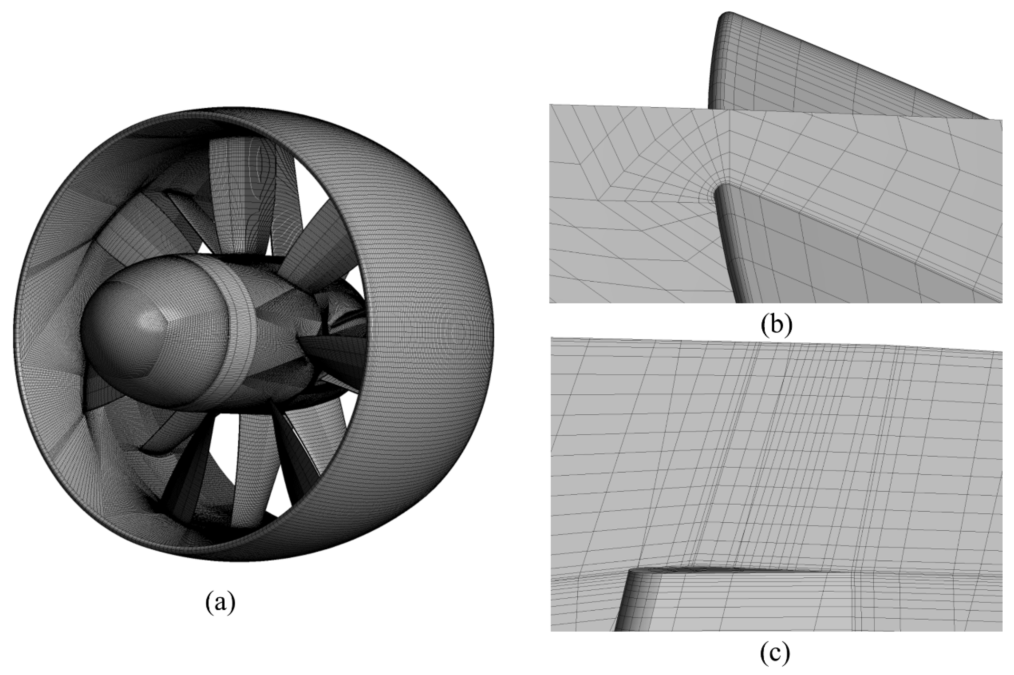
ANSYS ICEM software was used to generate the structured mesh and O-grid block was used around the rotor blade. In order to capture the vortex motion near the rotor blade and the inner wall of the duct, the boundary layer mesh of this part was further refined, where the tip clearance boundary layer is 20 layers and the blade wall boundary layer is 10 layers. The mesh around the stator blades was also optimized with 20 boundary layer nodes. Since the flow separation is more likely at the inlet and outlet of the duct, the number of boundary layer nodes near the duct, the diversion cap, and the wake hood was also increased. The final mesh distribution of the pump jet propeller is shown in Figure 5, where Figure 5a shows the mesh of the entire system of the pump-jet propeller, while Figure 5b,c show the boundary layers around the rotor blades and in the tip clearance area, respectively. In order to ensure a good transition of flow field information between different computational domains, the number of nodes on the interface between external flow field and rotor, rotor and stator, stator and external flow field is adjusted to be 105 order of magnitude.
The grid resolution of SST k-ω model is fine and the Y+ values should be less than 30. Y+ values around the pump-jet propeller are listed in Table 1:
2.5.3. Grid Independence Analysis
In order to eliminate the influence of insufficient number of grids on the computational accuracy, meanwhile avoid the waste of computing resources caused by excessive grids, it is mandatory to conduct the grid-independence analysis of the computational domain beforehand. Table 2 shows the comparison of different grid numbers for grid independence analysis. By increasing the number of boundary layer nodes, six sets of grids including 1.76 million, 3.36 million, 4.87 million, 6.37 million, 8.81 million, and 10.37 million are obtained. By comparing the thrust coefficient, torque coefficient, and propulsion efficiency of a different number of computational domain grids under design conditions, the most appropriate number of grids is concluded.
It can be seen from the table that as the number of grids increases, the margin between the propulsion efficiencies becomes smaller and smaller. Therefore, in order to obtain the flow field information near the wall more accurately and reduce computational resource consumption, the case of 8.81 million grid schemes is selected for numerical study in this paper.
3. Cavitation and Vortex Dynamics Analysis of Pump-Jet Propeller
3.1. Tip Vortex and Monitoring Points Positioning
In the rotor system of a pump-jet propeller, due to the tip clearance between the blade tip and the inner wall of the duct, vortices including the tip leakage vortices (TLV) and the tip separation vortices (TSV), occur among this area when the pump-jet propeller rotates at high speeds as shown in Figure 6. The formation of TLV is mainly influenced by two factors: pressure difference between pressure side and suction side of blades and relative movement between blade and wall. The formation of TSV is mainly influenced by the tip and wall boundary layer, so the track of TSV core is basically in the gap area of the tip while its position is close to the tip. The starting point of the TLV is the same as that of the TSV, but its trajectory gradually diffuses from the starting point of the TSV to the direction away from the blade wall, since the motion of the main flow field drives TLV to the main flow channel.
The research focus of this paper is on the analysis of the dynamic characteristics of the tip vortices, so it is an effective means to set monitoring points to measure the unsteady characteristics of the tip vortices. Based on the principle of minimum pressure [49], vortex cores in different axial positions of TLV and TSV are selected to monitor their pressure. The position of the vortex core is shown in Figure 7. The horizontal axis λ represents the projection of the chord length of the blade tip on the coordinate axis and the vertical axis represents the axial distance in the absolute coordinate system. Five and seven monitor points are taken from TLV and TSV, respectively. The monitor points of TLV are prefixed by LP while the monitor points of TSV are prefixed by SP.
In order to clearly compare the influence of cavitation on tip vortices before and after cavitation, the rotational speeds selected in this paper are 1250 rpm and 1750 rpm, corresponding J = 1.02 and J = 0.73, respectively. As shown in the Figure 8, peak propulsion efficiency with cavitation occurs at J = 1.02, and then the curve of efficiency begins to decrease. When the rotational speed increases to J = 0.73, the efficiency of cavitation condition is much lower than non-cavitation which is regarded as a severe cavitation scenario.
3.2. Slight cavitation at J = 1.02
3.2.1. Pressure fluctuation
In this work, non-dimensional parameter Cp is used to represent pressure pulsation, which is computed by:
where Cp is pressure coefficient, p is the local pressure, is the time average pressure, v is the incoming velocity. By calculation, the advance ratio J is equal to 1.02 and the cavitation number σ is equal to 3.98 for both non-cavitation and cavitation scenarios.
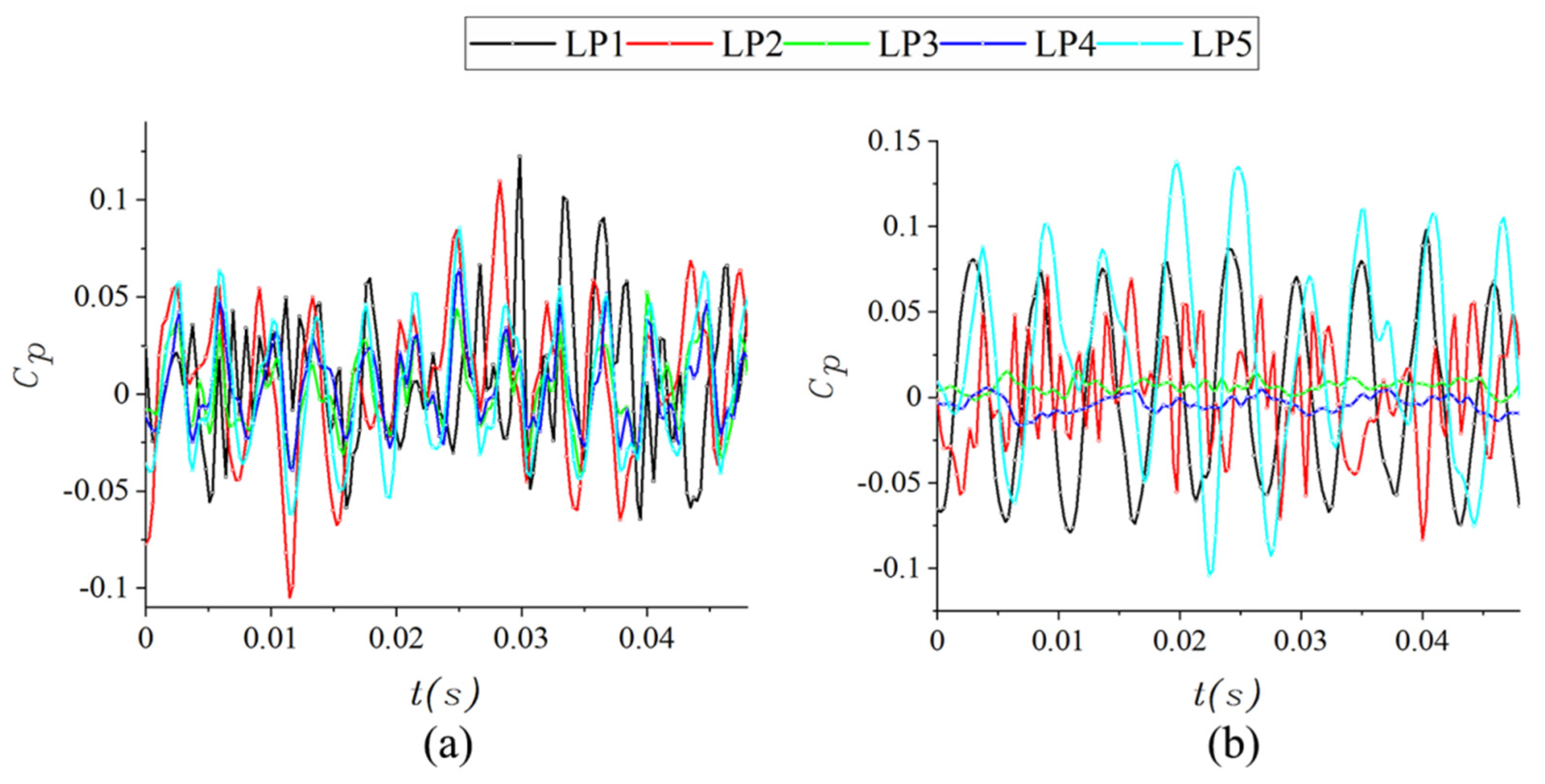
Figure 9 shows the time domain diagram of pressure pulsation before and after cavitation at TLV monitoring points. It can be found that when there is no cavitation, the peak and bottom of the five monitoring points of TLV appear almost at the same time, and the number of peak and bottom are the same showing evident regularity. In the time domain diagram after cavitation, LP1 and LP2 fluctuate disorderly with less evident regularity compared to LP4 and LP5, and the degree of disorder is less at LP3. It indicates that the slight cavitation has affected the middle position of the tip. By observing the fluctuations of LP4 and LP5, it can be found that the peak pressure coefficient after cavitation is twice high compared to that without cavitation. Figure 9b shows the secondary peak, which indicates that cavitation in the middle of the tip affects the flow field near the trailing edge of the blade.
Figure 10 presents frequency domain diagram of pressure fluctuation before and after cavitation at TLV monitoring points. The pressure fluctuations in Figure 10 are extremely distinctive before and after cavitation. The horizontal axis in this figure represents the multiples of the shaft frequency (SFM), and the value of the shaft frequency equals the rotational speed in r/s. It can be seen from Figure 10a that prior to the cavitation, the main frequency of the five monitoring points is 9 times the shaft frequency and the secondary frequency is four times the shaft frequency, which might be caused by the interaction between rotor blades and stator. After cavitation, LP1 is located in the core area of cavitation, so its pulsation has no apparent regularity. For LP2–LP5, their main and secondary main frequencies are still nine times and four times of the shaft frequency, respectively. Nevertheless, compared with the case without cavitation, the fluctuation components increase after cavitation, and low-frequency and high-frequency fluctuations also occur at the same time.
Figure 11 provides the results of pressure and vorticity changes before and after cavitation at TLV monitoring points. As can be seen from Figure 11, regardless of the existence of the cavitation, the pressure of the TLV core increases and the vorticity decreases from the tip inlet to the outlet. This is due to the fact that the TLV is in the developing stage at the tip leading edge, so the internal pressure of the vortex core is low and the vorticity is large. When it gradually decays and dissipates, the internal pressure of the vortex core gradually returns to the value of the mainstream and the vorticity will decrease accordingly. When cavitation occurs, because of the low-pressure area exists around vortex cores, the pressure inside the vortex core will further decrease. Furthermore, cavitation bubbles will increase the pressure gradient in the tip cap, which may cause the velocity curl to come up, and then the vorticity enlarges.
3.2.2. Evolution of TLV
Figure 12 shows the evolution of tip vortex in a rotating period. The TLV and TSV shown are based on the Q-criterion ISO-surface. From the figure, it can be seen that after 1/8 cycle of rotor rotation, TSV has begun to merge into TLV. By 2/8 cycle, TSV has fully merged and then both TLV and TSV begin to dissipate. Because of the relative motion between blade tip and end wall, there is induced vortex formed near the blade suction surface. TLV is generated at 5/8 cycles and the induced vortices are separated from TSV. As the rotor rotates, the induced vortices gradually converge towards TLV. After 1/3 cycles, the induced vortices are fully integrated with TLV. It should be noted that the main frequency in the figure is equal to the passing frequency of the stator.
Figure 13 shows periodic evolution of vortices under cavitation at J = 1.02. As shown in Figure 13, at T0 without the cavitation, the length of the vortices extends to the trailing edge of the blade. At 1/8 cycle, the non-cavitation TSV has begun to merge into the TLV, while at cavitation conditions, the two vortices have completely merged at 2/8 cycle, which indicates that the merging time of TSV to the TLV under cavitation is between 1/8 cycle and 2/8 cycle. The cavitation can delay the merging process of vortices. This conclusion can be proved at 5/8 cycles: TSV has already started to separate the induced vortices which began to move towards TLV in non-cavitation condition. However, there are almost no induced vortices for the cavitation until 6/8 cycles. Therefore, by comparing the vortex shape evolution before and after cavitation, it can be deduced that cavitation will make TLV extend to the trailing edge of blade, while delaying the fusion between TSV and TLV.
Figure 14 presents the Z-direction component contour of stretching term at two adjacent times before and after cavitation. The stretching term comes from the vorticity transport equation which is introduced as follows:
where ω is the vorticity, ρ is the local fluid density, p is the local pressure, V is the flow velocity, and ν is the dynamic viscosity. The definition of vorticity ω is:
In Equation (17), the stretching term (ω·∇)V on the right-hand side describes the stretching or tilting of vorticity due to the flow velocity gradients. The expansion term ω(∇·V) describes stretching of vorticity due to flow compressibility. The term is the baroclinic term. It accounts for the changes in the vorticity due to the intersection of density and pressure surfaces. The viscous dissipation term, ν∇2ω, accounts for the diffusion of vorticity due to the viscous effects [50,51]. Because the fluid flow medium used in this paper is incompressible, the baroclinic and expansion terms are zero. Moreover, since the viscous dissipation effect can be neglected in high Reynolds number fluid, only the stretching term is analyzed in this paper.
It can be found that the stretching component value in the core region of TLV is positive while the surrounding is negative. The stretching value is positive in TSV core region, and the positive distribution extends to TLV core region. However, the stretching component around the TSV core is negative, showing that there is a velocity gradient with opposite rate of change around the vortex core. According to the distribution of vortex cores, the tip vortices of 2/8T are both longer than those of 1/8T to the blade trailing edge, indicating the tip vortex is in the development stage. There is no evident distinction between two moments under the condition of no cavitation. However, when the cavitation occurs, it is apparent that the positive distribution range of stretching term increases which indicates that cavitation, will aggravate the stretching and bending of tip vortex.
3.3. Severe Cavitation at J = 0.73
3.3.1. Pressure Fluctuation
Figure 15 depicts the time domain diagram of pressure fluctuation before and after cavitation at TLV monitoring points. By calculation, the advance ratio J is equal to 0.73 and the cavitation number σ is equal to 3.98 for both non-cavitation and cavitation scenarios. As can be seen in the figure, there is a big difference in the time domain diagram of pressure fluctuation before and after cavitation. It is most evident that after cavitation, the fluctuation amplitude of LP3 and LP4 is much smaller than that of other monitoring points. In addition, the pressure fluctuation amplitude of all monitoring points was increased compared with that before cavitation. LP1 fluctuates irregularly before cavitation, showing that the difference between the peak and bottom is always changing at different times, which change into sine curve after cavitation. The pressure change of LP2 is more disordered after cavitation, and the number of peak and bottom is significantly increased than that before cavitation. The fluctuation amplitude of LP5 before cavitation is basically similar to that of LP3 and LP4, but it has the largest pressure fluctuation amplitude after cavitation.
Figure 16 shows the pressure fluctuation of TLV monitoring point before and after cavitation at J = 0.73. First of all, the primary frequency has not changed which is still 9 times the shaft frequency, but the secondary frequency is not all 4 times the shaft frequency. Except at LP3, the secondary dominant frequency of the other four monitoring points is replaced by 0.1 times the shaft frequency. However, the entire secondary frequency is replaced by low multiples of the shaft frequency. Especially at LP3 and LP4, the main frequency is 0.1 times the shaft frequency, while 9 times the shaft frequency becomes the secondary frequency. The amplitudes of LP3 and LP4 in Figure 14b are far less than those of the other three monitor points, and the amplitudes corresponding to the main frequency of LP2 are also smaller than those under the condition of no cavitation. On one hand, the three monitoring points are located in the serious cavitation area, and the fluid is filled with bubbles, so the turbulence fluctuation of water will be weakened. On the other hand, when cavitation occurs, the position of the vortex core will shift compared with that without cavitation. Therefore, LP2–LP4 may be just in the region around the vortex core when cavitation occurs, which is filled by bubbles, resulting in the reduced intensity of pressure fluctuation.
3.3.2. Evolution of TLV
Figure 17 and Figure 18 shows periodic evolution of vortices before and after cavitation at J = 0.73, respectively. Compared with Figure 12, the periodicity of TLV in Figure 17 is shorter. The shape of vortex at 6/8T is similar to that at T0, which indicates that the high rotational speed will shorten the period of vortex. In Figure 18, the TLV with cavitation is evidently different from that of non-cavitation. Firstly, the vortex area marked by black dotted line in the figure is not found at J = 1.02 and J = 0.73 without cavitation. Moreover, this vortex runs through the whole rotation cycle, indicating that when severe cavitation occurs, a third type of vortex will appear at the trailing edge of the tip, which is located between TLV and TSV and is generated by the tip and transported to TLV. Moreover, it can be found that even if the TLV breaks at the leading edge of the tip, the trail of TLV still appears at the trailing edge of the tip, and its diameter is larger than that of the leading edge. From the previous analysis, it can be seen that severe cavitation will lead to the second development of TLV at the tip trailing edge, and its pulsation comes from TSV.
Figure 19 shows the change of Q at 1/8 cycle before and after cavitation at J = 0.73. Here, it can also be seen that TLV and TSV are separated from each other near the trailing edge of the blade tip without cavitation, and the distribution of TLV tends to expand in the stream-wise direction. When cavitation occurs, the area of TLV in the front and middle edge of blade tip is smaller than that of non-cavitation. TLV and TSV are not completely separated near the trailing edge of blade tip. There is a clear red ribbon vortex connecting TLV and TSV, and there is a blue area around the red ribbon vortex. It shows that the fluid is stretched between TLV and TSV near the trailing edge of blade tip when severe cavitation occurs.
Figure 20 shows the contrast of the stretching term of vorticity transport equation before and after cavitation. It can be found that the stretching term is positive in the region of the vortex core, but negative around the core, indicating that the fluid around the core will be stretched and compressed. Compared with before and after cavitation, it can be found that there is a positive stretching term between TLV and TSV in the section near the blade trailing edge, which indicates that there is a stronger interaction between TSV and TLV at the blade trailing edge when severe cavitation occurs.
3.4. Comparison of J = 1.02 and J = 0.73 Results
In order to investigate the mechanism by which cavitation bubbles affect the tip vortex, it is necessary to compare the results of different rotational speeds. As shown in Figure 21, the TLV trajectory changes as the rotational speed increases from J = 1.02 to J = 0.73.
When cavitation occurs at J = 1.02, the trend of TLV trajectory almost coincides with that of non-cavitation in the upper and middle part of the tip. However, as it moves towards the outlet of the rotor, the cavitation vortex core firstly approaches the suction side of the blade and then shifts away from it. It is obvious that the track of the TLV will be far away from the suction side of the blade when the rotational speed is high, so it can be inferred that the starting point of the TLV will move towards the leading edge of the tip as the rotational speed increases. Differing from the TLV vortex core track at J = 1.02, there is little coincidence of TLV vortex core before and after cavitation at high rotational speed. In addition, when cavitation occurs, the vortex core first moves away from the blade in the downstream area near the tip, which then shifts towards it.
In order to investigate the intensity changes of TLV under different cavitation levels, the vortex cores of TLV are extracted from 8 axial sections along the axial heights of 6 mm, 4 mm, 2 mm, 0 mm, −2 mm, −4 mm, −6 mm and −8 mm, named P1~P8 respectively, and their vorticity changes (represented by Q value) are shown in Figure 22. It can be found that Q decreases gradually in the stream-wise direction at J = 1.02 without cavitation and then hardly changes at the trailing edge of the tip due to the dissipated tip vortices. Then, when the pump-jet propeller cavitates at this rotational speed, the vorticity strength of P1 and P2 increases sharply, and the Q is almost twice as much as that of non-cavitation. It indicates that under slight cavitation, bubbles promote the strength of tip vortices. The Q value under cavitation is much larger than that under non-cavitation up to the trailing edge of the blade, showing that the influence of cavitation bubbles on the tip vortices always exists along the tip clearance near the blade tip. As the rotational speed increases to 1750 rpm, the TLV intensity without cavitation becomes more intense. That can be explained as the faster the rotor rotates, the bigger the speed gradient in the tip vortex region and the higher the curl. At J = 0.73, the bubbles cover almost the entire suction side of the blade, so that the fluid near the tip is replaced by bubbles. In severe cavitation condition, Q rises from P5 due to the bubbles filling the surrounding water. Bubbles appear because of the low-pressure zone, and the range of the low-pressure area around the vortex core is larger than that without cavitation, which promotes the generation of the tip vortex. Since the driving force of tip vortices comes from the pressure gradient, the cavitation will increase the pressure gradient around the vortices core, which makes TLV develop for a second time.
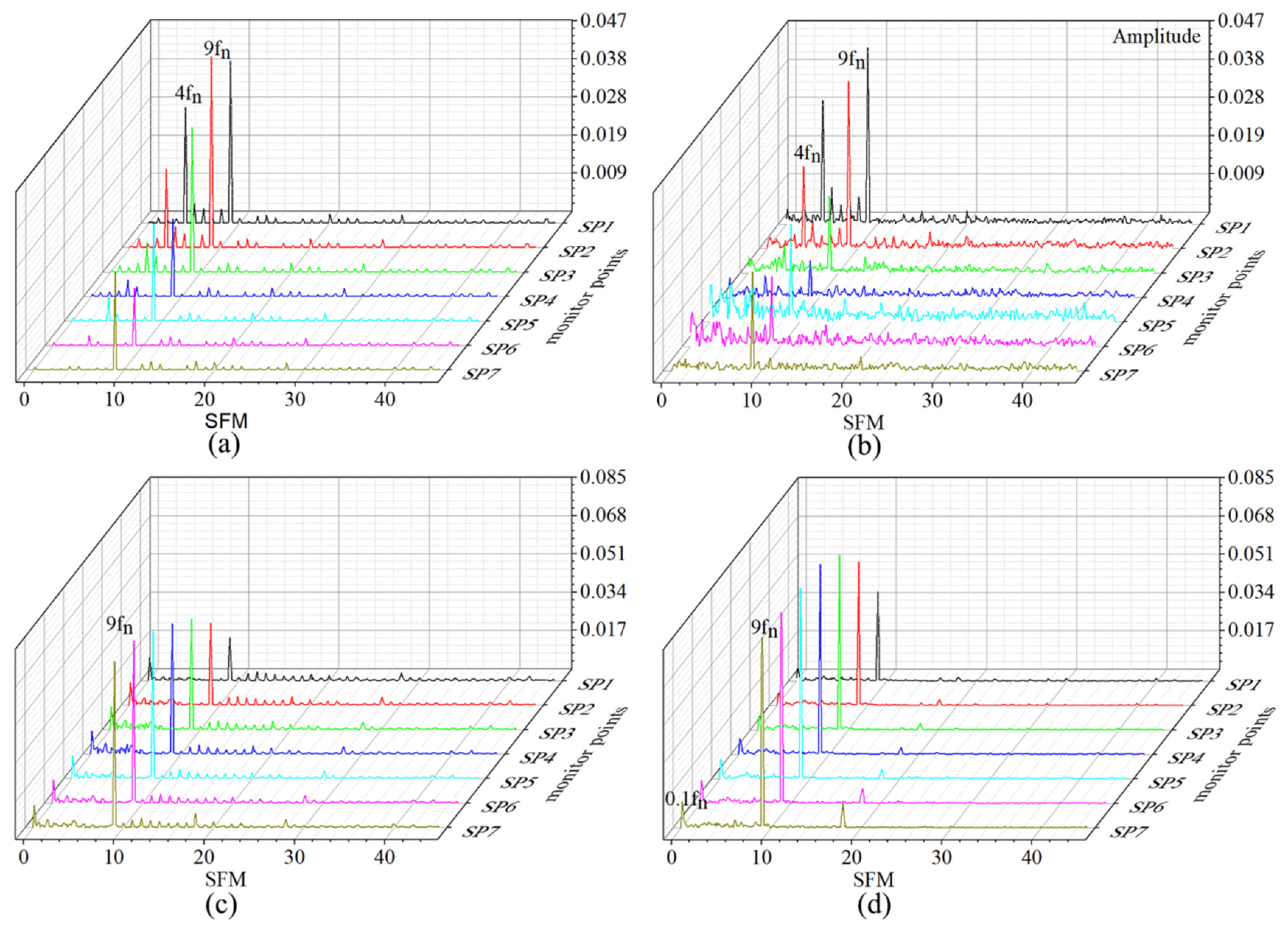
From Figure 23, it can be found that the main frequency of TSV is 9 times the shaft frequency regardless of the cavitation situation. When there is no cavitation, the sub-main frequency of SP1-SP5 is 4 times the shaft frequency. The amplitude of 4 times the shaft frequency in SP6 and SP7 decreases, which is almost negligible compared with the amplitude of the main frequency. When cavitation occurs, except that the amplitude corresponding to the main frequency of SP1 is higher than that of non-cavitation, the most obvious difference is that many low frequency pulsations occur in the cavitation TSV, which is most evident in SP5 and SP6. In addition, the corresponding amplitudes of the main frequencies of SP3 and SP4 are much lower than those without cavitation. It is because when slight cavitation occurs inside the rotor, the bubbles extend to the tip clearance area where the SP4 is located, so that the fluid in this area is filled with bubbles, and as a result, the corresponding amplitude of the main frequency fluctuation is reduced.
At J = 0.73, the main frequency is still 9 times the shaft frequency, but the secondary frequency is replaced by 0.1 times the shaft frequency. In addition, along the direction of flow, the amplitude of main frequency increases in turn, which increases further when cavitation occurs. Moreover, the difference of the corresponding amplitude of the main frequency at each monitor point is very small, indicating that turbulent instability of TSV increases when severe cavitation occurs.
4. Conclusions
In the present work, on the basis of the DES turbulence model and Zwart–Gerber–Belamri cavitation model, the shape and dynamic characteristics of TLV and TSV of a pump-jet propeller under slight and severe cavitation conditions were studied. The vorticity equation and two vortex recognition methods were employed in this study and through comparative analysis, it found that:
- At J = 1.02, the vortices at cavitation extend towards the trailing edge of the blade compared with the vortices at non-cavitation, and the integration time of TLV and TSV is delayed. The main frequency of the TLV vortex core is nine times the shaft frequency and the secondary frequency is 4 times the shaft frequency when the cavitation is mild. However, low-frequency and high-frequency pulsations occur at the severe cavitation. By using the stretching term in the vorticity equation to analyze the dynamic characteristics of TLV, it is found that cavitation will intensify the stretching and bending of the tip vortices.
- At J = 0.73, the main frequency of the vortex core is still nine times the shaft frequency, but the secondary main frequency is almost all replaced by 0.1 times the shaft frequency. After cavitation occurs, a third type of vortex appears near the trailing edge of the blade, which is located between TLV and TSV while generated by the tip and moved towards TLV. The stretch term contour shows that the TLV and TSV are independent at the leading and middle parts of the blades. When cavitation occurs, there are red ribbon vortexes at the trailing edge of the tip that connect the TLV and TSV.
- When slight cavitation occurs, the cavitation promotes the intensity of the tip vortices and the Q is much higher. Furthermore, bubbles promote the strength of tip vortices and the Q at cavitation is much larger than that at non-cavitation. As the rotational speed increases, the cavitation area on the blade surface will increase further than at low rotational speeds, since the increase in velocity will lead to a decrease in local pressure.
- After cavitation, the position of the TLV vortex core will deviate from that before cavitation. When slight cavitation occurs, the position of the vortex core hardly changes in the upper and middle reaches of the tip. However, along the stream-wise direction, the vortex core first moves towards the suction side of blade and then moves away from it. When severe cavitation occurs, the position of the vortex core deviates considerably from that before cavitation, and the trend of deviation is opposed to that of slight cavitation.
- The pressure fluctuation of the TSV vortex core shows that, at J = 1.02, the pulsation intensity of the cavitation TSV near the middle of the tip is much lower than that near the leading edge of the suction side of the blade. This indicates that although cavitation only occurs near the suction side, its influence on the flow field extends to the middle area of the tip. At J = 0.73, the amplitude of the main frequency at all monitoring points of the TSV is increased and the entire TSV is affected by cavitation. In addition, the turbulent instability of TSV is more severe. For future work, similar optimization as in references [52,53] for the pump-jet impeller can be performed to enhance the general propulsion efficiency of the device and to save power.
Author Contributions
Conceptualization, J.Y. and L.W.; methodology, Y.C.; software, Y.C. and Y.Z.; investigation, Y.F. and J.X.; writing-original draft preparation, Y.C. and L.W.; writing—review and editing, L.W. and R.L. All authors have read and agreed to the published version of the manuscript.
Funding
This research was funded by Institute of Fluid Engineering Equipment, Natural Science Foundation of Jiangsu Province (Grant No. BK20180879), High-level Talent Research Foundation of Jiangsu University (Grant No. 18JDG012), National Key Research and Development Plan Project (Grant No. 2018YFB0606103) and Construction of Dominant Disciplines in Colleges and Universities and Universities in Jiangsu (PAPD).
Conflicts of Interest
The authors declare no conflict of interest. The funders had no role in the design of the study; in the collection, analyses, or interpretation of data; in the writing of the manuscript, or in the decision to publish the results
References
- Carlton, J. Marine Propellers and Propulsion; Butterworth-Heinemann: Oxfordshire, British, 2018. [Google Scholar]
- Stanic, S.; Dahlburg, R.; Caruthers, J. Bubble number densities in the wake of a propeller and a pump jet ship. In Proceedings of the 2013 Oceans—San Diego, San Diego, CA, USA, 23–27 September 2013. [Google Scholar]
- Buckland, H.C.; Masters, I.; Orme, J.A.; Baker, T. Cavitation inception and simulation in blade element momentum theory for modelling tidal stream turbines. Proc. Inst. Mech. Eng. Part A J. Power Energy 2013, 227, 479–485. [Google Scholar] [CrossRef]
- Hayden, B.J. Two-Dimensional Analysis of Rotor Suction and the Impact on Rotor-Stator Interaction Noise; Massachusetts Institute of Technology: Cambridge, MA, USA, 1994. [Google Scholar]
- Suryanarayana, C.; Satyanarayana, B.; Ramji, K.; Saiju, A. Experimental evaluation of pumpjet propulsor for an axisymmetric body in wind tunnel. Int. J. Nav. Archit. Ocean Eng. 2010, 2, 24–33. [Google Scholar] [CrossRef] [Green Version]
- Suryanarayana, C.; Satyanarayana, B.; Ramji, K. Performance evaluation of an underwater body and pumpjet by model testing in cavitation tunnel. Int. J. Nav. Archit. Ocean Eng. 2010, 2, 57–67. [Google Scholar] [CrossRef] [Green Version]
- Suryanarayana, C.; Satyanarayana, B.; Ramji, K.; Rao, M.N. Cavitation studies on axi-symmetric underwater body with pumpjet propulsor in cavitation tunnel. Int. J. Nav. Archit. Ocean Eng. 2010, 2, 185–194. [Google Scholar] [CrossRef] [Green Version]
- Shirazi, A.T.; Nazari, M.R.; Manshadi, M.D. Numerical and experimental investigation of the fluid flow on a full-scale pump jet thruster. Ocean Eng. 2019, 182, 527–539. [Google Scholar] [CrossRef]
- Das, H.; Jayakumar, P.; Saji, V.; Yerram, R. CFD examination of interaction of flow on high-speed submerged body with pumpjet propulsor. In Proceedings of the HIPER 06: 5th International Conference on High-Performance Marine Vehicles, Launceston, Australia, 8–10 November 2006; p. 466. [Google Scholar]
- Dong, Y.; Duan, X.; Feng, S.; Shao, Z. Numerical Simulation of the Overall Flow Field for Underwater Vehicle with Pump Jet Thruster. Procedia Eng. 2012, 31, 769–774. [Google Scholar] [CrossRef] [Green Version]
- Ahn, S.J.; Kwon, O.J. Numerical investigation of a pump-jet with ring rotor using an unstructured mesh technique. J. Mech. Sci. Technol. 2015, 29, 2897–2904. [Google Scholar] [CrossRef]
- Shi, Y.; Pan, G.; Huang, Q.; Du, X. Numerical Simulation of Cavitation Characteristics for Pump-jet Propeller. In Proceedings of the XXVI Iupap Conference on Computational Physics, Boston, MA, USA, 11–14 August 2014; Volume 640. [Google Scholar]
- Lin, L.; Guang, P. Numerical Simulation Analysis of Unsteady Cavitation Performance of a Pump-jet Propulsor. J. Shanghai Jiaotong Univ. 2015, 21. [Google Scholar] [CrossRef]
- Pan, G.; Lu, L. Numerical investigation of a pumpjet propulsor based on CFD. Int. J. Control Autom. 2015, 8, 225–234. [Google Scholar] [CrossRef] [Green Version]
- Lu, L.; Gao, Y.; Li, Q.; Du, L. Numerical investigations of tip clearance flow characteristics of a pumpjet propulsor. Int. J. Nav. Archit. Ocean Eng. 2018, 10, 307–317. [Google Scholar] [CrossRef]
- Qin, D.; Pan, G.; Huang, Q.; Zhang, Z.; Ke, J. Numerical Investigation of Different Tip Clearances Effect on the Hydrodynamic Performance of Pumpjet Propulsor. Int. J. Comput. Methods 2018, 15. [Google Scholar] [CrossRef] [Green Version]
- Li, H.; Pan, G.; Huang, Q.; Shi, Y. Numerical Prediction of the Pumpjet Propulsor Tip Clearance Vortex Cavitation in Uniform Flow. J. Shanghai Jiaotong Univ. (Sci.) 2019, 1–13. [Google Scholar] [CrossRef]
- Wang, C.; Weng, K.; Guo, C.; Gu, L. Prediction of hydrodynamic performance of pump propeller considering the effect of tip vortex. Ocean Eng. 2019, 171, 259–272. [Google Scholar] [CrossRef]
- Qiu, C.; Huang, Q.; Pan, G.; Shi, Y.; Dong, X. Numerical simulation of hydrodynamic and cavitation performance of pumpjet propulsor with different tip clearances in oblique flow. Ocean Eng. 2020, 209. [Google Scholar] [CrossRef]
- Gong, J.; Guo, C.-Y.; Zhao, D.-G.; Wu, T.-C.; Song, K.-W. A comparative DES study of wake vortex evolution for ducted and non-ducted propellers. Ocean Eng. 2018, 160, 78–93. [Google Scholar] [CrossRef]
- Huang, J.; Zhang, L.; Wang, W.; Yao, J. Fine simulation of 3-D unsteady flows in a francis hydro-turbine on detached eddy simulation. In Proceedings of the Zhongguo Dianji Gongcheng Xuebao (Proceedings of the Chinese Society of Electrical Engineering), Guizhou, China, 27 September 2011; pp. 83–89. [Google Scholar]
- Dawi, A.H.; Akkermans, R.A. Direct noise computation of a generic vehicle model using a finite volume method. Comput. Fluids 2019, 191, 104243. [Google Scholar] [CrossRef]
- Dawi, A.H.; Akkermans, R.A. Spurious noise in direct noise computation with a finite volume method for automotive applications. Int. J. Heat Fluid Flow 2018, 72, 243–256. [Google Scholar] [CrossRef]
- Dawi, A.H.; Akkermans, R.A. Direct and integral noise computation of two square cylinders in tandem arrangement. J. Sound Vib. 2018, 436, 138–154. [Google Scholar] [CrossRef]
- Sun, S.; Wang, C.; Guo, C.; Zhang, Y.; Sun, C.; Liu, P. Numerical study of scale effect on the wake dynamics of a propeller. Ocean Eng. 2020, 196. [Google Scholar] [CrossRef]
- Lungu, A. A DES-SST Based Assessment of Hydrodynamic Performances of the Wetted and Cavitating PPTC Propeller. J. Mar. Sci. Eng. 2020, 8, 297. [Google Scholar] [CrossRef] [Green Version]
- Li, H.; Huang, Q.; Pan, G.; Dong, X. The transient prediction of a pre-swirl stator pump-jet propulsor and a comparative study of hybrid RANS/LES simulations on the wake vortices. Ocean Eng. 2020, 203. [Google Scholar] [CrossRef]
- Li, G.-N.; Zhang, J.; Zhang, G.-P.; Lu, L.-Z. Propeller wake analysis by means of PIV in large water tunnel. Acta Aerodyn. Sin. 2010, 28, 503–508. [Google Scholar]
- Zhang, D.; Shi, W.; Van Esch, B.B.; Shi, L.; Dubuisson, M. Numerical and experimental investigation of tip leakage vortex trajectory and dynamics in an axial flow pump. Comput. Fluids 2015, 112, 61–71. [Google Scholar] [CrossRef]
- Hao, Y.; Tan, L. Symmetrical and unsymmetrical tip clearances on cavitation performance and radial force of a mixed flow pump as turbine at pump mode. Renew. Energy 2018, 127, 368–376. [Google Scholar] [CrossRef]
- Zhang, D.; Shi, W.; Pan, D.; Dubuisson, M. Numerical and Experimental Investigation of Tip Leakage Vortex Cavitation Patterns and Mechanisms in an Axial Flow Pump. J. Fluids Eng. Trans. Asme 2015, 137. [Google Scholar] [CrossRef]
- Wen, Z.; Liu, P.; Hao, G. Review of transition prediction methods. J. Exp. Fluid Mech. 2014, 28, 1–12. [Google Scholar]
- Nakisa, M.; Abbasi, M.J.; Amini, A.M. Assessment of marine propeller hydrodnamic performance in open water via CFD. In Proceedings of the 7th International Conference on Marine Technology (MARTEC 2010), Dhaka, Bangladesh, 11 December 2010. [Google Scholar]
- Ji, B.; Luo, X.-w.; Wu, Y.-l.; Liu, S.-h.; Xu, H.-y.; Oshima, A. Numerical investigation of unsteady cavitating turbulent flow around a full scale marine propeller. J. Hydrodyn. 2010, 22, 705–710. [Google Scholar] [CrossRef]
- Heydari, M.; Sadat-Hosseini, H. Analysis of propeller wake field and vortical structures using k—Omega SST Method. Ocean Eng. 2020, 204. [Google Scholar] [CrossRef]
- Motallebi-Nejad, M.; Bakhtiari, M.; Ghassemi, H.; Fadavie, M. Numerical analysis of ducted propeller and pumpjet propulsion system using periodic computational domain. J. Mar. Sci. Technol. 2017, 22, 559–573. [Google Scholar] [CrossRef]
- Bennaya, M.; Gong, J.F.; Hegaze, M.M.; Zhang, W.P. Numerical simulation of marine propeller hydrodynamic performance in uniform inflow with different turbulence models. In Applied Mechanics and Materials; Trans Tech Publications Ltd.: Bäch SZ, Switzerland, 2013; Volume 389, pp. 1019–1025. [Google Scholar]
- Gu, Y.; Pei, J.; Yuan, S.; Wang, W.; Zhang, F.; Wang, P.; Appiah, D.; Liu, Y. Clocking effect of vaned diffuser on hydraulic performance of high-power pump by using the numerical flow loss visualization method. Energy 2019, 170, 986–997. [Google Scholar] [CrossRef]
- Gu, Y.; Pei, J.; Yuan, S.; Zhang, J. A Pressure Model for Open Rotor–Stator Cavities: An Application to an Adjustable-Speed Centrifugal Pump with Experimental Validation. J. Fluids Eng. 2020, 142. [Google Scholar] [CrossRef]
- Yu, H.; Zhang, Z.; Hua, H. Numerical investigation of tip clearance effects on propulsion performance and pressure fluctuation of a pump-jet propulsor. Ocean Eng. 2019, 192. [Google Scholar] [CrossRef]
- Yu, H.; Duan, N.; Hua, H.; Zhang, Z. Propulsion performance and unsteady forces of a pump-jet propulsor with different pre-swirl stator parameters. Appl. Ocean Res. 2020, 100. [Google Scholar] [CrossRef]
- Spalart, P.R. Comments on the feasibility of LES for wings, and on a hybrid RANS/LES approach. In Proceedings of the First AFOSR International Conference on DNS/LES, Louisiana Tech University, Ruston, LA, USA, 4–8 August 1997. [Google Scholar]
- Yan, H.; Li, Q.; Zhang, Y.; Shi, H.X.; Vnenkovskaia, V. Optimization of cavitating flow characteristics on rbss of waterjet pumps. Int. J. Simul. Model. 2018, 17, 271–283. [Google Scholar] [CrossRef]
- Sikirica, A.; Carija, Z.; Kranjcevic, L.; Lucin, I. Grid Type and Turbulence Model Influence on Propeller Characteristics Prediction. J. Mar. Sci. Eng. 2019, 7, 374. [Google Scholar] [CrossRef] [Green Version]
- Xu, S.; Long, X.-p.; Ji, B.; Li, G.-b.; Song, T. Vortex dynamic characteristics of unsteady tip clearance cavitation in a waterjet pump determined with different vortex identification methods. J. Mech. Sci. Technol. 2019, 33, 5901–5912. [Google Scholar] [CrossRef]
- Ramakrishna, S.; Ramakrishna, V.; Ramakrishna, A.; Ramji, K. CFD Analysis of a Propeller Flow and Cavitation. Int. J. Comput. Appl. 2012, 55, 26–33. [Google Scholar] [CrossRef]
- Felli, M.; Camussi, R.; di Felice, F. Mechanisms of evolution of the propeller wake in the transition and far fields. J. Fluid Mech. 2011, 682, 5–30. [Google Scholar] [CrossRef] [Green Version]
- Rijpkema, D.; Vaz, G. Viscous Flow Computations on Propulsors: Verification, Validation and Scale Effects. In Proceedings of the Rina Marine CFD, London, UK, 22–23 March 2011. [Google Scholar]
- Epps, B. Review of vortex identification methods. In Proceedings of the 55th AIAA Aerospace Sciences Meeting, Grapevine, TX, USA, 9–13 January 2017; p. 0989. [Google Scholar]
- Available online: https://en.wikipedia.org/wiki/Vorticity_equation (accessed on 30 July 2020).
- Kozlov, V.V. Dynamical Systems X: General Theory of Vortices; Springer: Berlin/Heidelberg, Germany, 2013; Volume 67. [Google Scholar]
- Wang, L.; Asomani, S.; Yuan, J.; Appiah, D. Geometrical Optimization of Pump-As-Turbine (PAT) Impellers for Enhancing Energy Efficiency with 1-D Theory. Energies 2020, 13, 4120. [Google Scholar] [CrossRef]
- Asomani, S.; Yuan, J.; Wang, L.; Appiah, D. The Impact of Surrogate Models on the Multi- Objective Optimization of Pump-As-Turbine (PAT). Energies 2020, 13, 2271. [Google Scholar] [CrossRef]
Figure 1.
Computation domain.

Figure 2.
Cavitation calculation compared with experiments (J = 0.71).

Figure 3.
Pump-jet propeller model.

Figure 4.
Computational domain.

Figure 5.
Pump-jet propeller mesh and rotor local mesh: (a) mesh of pump-jet propeller (b) local boundary layers near the blades (c) local boundary layers in the tip clearance.
Figure 5.
Pump-jet propeller mesh and rotor local mesh: (a) mesh of pump-jet propeller (b) local boundary layers near the blades (c) local boundary layers in the tip clearance.

Figure 6.
TLV and TSV schematics at J = 1.02: (a) streamline of Tip Leakage Vortex (TLV) (b) streamline of Tip Separation Vortex (TSV).
Figure 6.
TLV and TSV schematics at J = 1.02: (a) streamline of Tip Leakage Vortex (TLV) (b) streamline of Tip Separation Vortex (TSV).

Figure 7.
Diagram of the monitoring points positioning (a) rotor blades (b) location of monitor points.
Figure 7.
Diagram of the monitoring points positioning (a) rotor blades (b) location of monitor points.

Figure 8.
Comparison of propulsion efficiency of pump-jet propeller before and after cavitation at different speeds.
Figure 8.
Comparison of propulsion efficiency of pump-jet propeller before and after cavitation at different speeds.

Figure 9.
Time domain diagram of pressure pulsation before and after cavitation at TLV monitoring points (a) non-cavitation (b) cavitation.
Figure 9.
Time domain diagram of pressure pulsation before and after cavitation at TLV monitoring points (a) non-cavitation (b) cavitation.

Figure 10.
Frequency domain diagram of pressure fluctuation before and after cavitation at TLV monitoring points (a) non-cavitation (b) cavitation.
Figure 10.
Frequency domain diagram of pressure fluctuation before and after cavitation at TLV monitoring points (a) non-cavitation (b) cavitation.

Figure 11.
Pressure and vorticity changes before and after cavitation at TLV monitoring points.

Figure 12.
Periodic evolution of vortices under non-cavitation at J = 1.02, Q = 0.01.

Figure 13.
Periodic evolution of vortices under cavitation at J = 1.02, Q = 0.01.

Figure 14.
Z-direction component contour of stretching term at two adjacent times, (a) 1/8T non-cavitation (b) 1/8T cavitation (c) 2/8T non-cavitation (d) 2/8T cavitation.
Figure 14.
Z-direction component contour of stretching term at two adjacent times, (a) 1/8T non-cavitation (b) 1/8T cavitation (c) 2/8T non-cavitation (d) 2/8T cavitation.

Figure 15.
Time domain diagram of pressure fluctuation before and after cavitation at TLV monitoring points. (a) non-cavitation (b) cavitation.
Figure 15.
Time domain diagram of pressure fluctuation before and after cavitation at TLV monitoring points. (a) non-cavitation (b) cavitation.

Figure 16.
Pressure fluctuation of TLV monitoring point before and after cavitation at J = 0.73. (a) non-cavitation (b) cavitation.
Figure 16.
Pressure fluctuation of TLV monitoring point before and after cavitation at J = 0.73. (a) non-cavitation (b) cavitation.

Figure 17.
Periodic evolution of vortices under non-cavitation at J = 0.73, Q = 0.01.

Figure 18.
Periodic evolution of vortices at under cavitation J = 0.73, Q = 0.01.

Figure 19.
Change of Q at 1/8 cycle at J = 0.73 (a) non-cavitation (b) cavitation.

Figure 20.
Z-direction component contour of stretching term at J = 0.73, (a) non-cavitation (b) cavitation.
Figure 20.
Z-direction component contour of stretching term at J = 0.73, (a) non-cavitation (b) cavitation.

Figure 21.
Variation of TLV core trajectory with rotational speed and cavitation.

Figure 22.
Vorticity variation of TLV core before and after cavitation at J = 1.02 and J = 0.73.

Figure 23.
Frequency domain diagram of pressure fluctuation before and after cavitation at TSV monitoring points (a) J = 1.02 non-cavitation (b) J = 1.02 cavitation (c) J = 0.73 non-cavitation (d) J = 0.73 cavitation.
Figure 23.
Frequency domain diagram of pressure fluctuation before and after cavitation at TSV monitoring points (a) J = 1.02 non-cavitation (b) J = 1.02 cavitation (c) J = 0.73 non-cavitation (d) J = 0.73 cavitation.


Table 1.
Average Y+ of rotor and stator components.
| Parts | Y Plus |
|---|---|
| rotor blades | 12 |
| rotor wall | 20.5 |
| stator blades | 2.9 |
| stator wall | 16.8 |
Table 2.
Comparison of different grid numbers for grid independence analysis.
| J | Number of Grids | KT | KQ | η |
|---|---|---|---|---|
| 1.02 | 1,768,631 | 0.119 | 0.036 | 53.66% |
| 3,364,892 | 0.115 | 0.0329 | 56.7% | |
| 4,873,435 | 0.121 | 0.0355 | 55.33% | |
| 6,371,002 | 0.119 | 0.0357 | 54.11% | |
| 8,812,531 | 0.120 | 0.036 | 54.11% | |
| 10,371,656 | 0.121 | 0.0358 | 54.87% |
© 2020 by the authors. Licensee MDPI, Basel, Switzerland. This article is an open access article distributed under the terms and conditions of the Creative Commons Attribution (CC BY) license (http://creativecommons.org/licenses/by/4.0/).
Share and Cite
MDPI and ACS Style
Yuan, J.; Chen, Y.; Wang, L.; Fu, Y.; Zhou, Y.; Xu, J.; Lu, R. Dynamic Analysis of Cavitation Tip Vortex of Pump-Jet Propeller Based on DES. Appl. Sci. 2020, 10, 5998. https://doi.org/10.3390/app10175998
AMA Style
Yuan J, Chen Y, Wang L, Fu Y, Zhou Y, Xu J, Lu R. Dynamic Analysis of Cavitation Tip Vortex of Pump-Jet Propeller Based on DES. Applied Sciences. 2020; 10(17):5998. https://doi.org/10.3390/app10175998
Chicago/Turabian StyleYuan, Jianping, Yang Chen, Longyan Wang, Yanxia Fu, Yunkai Zhou, Jian Xu, and Rong Lu. 2020. "Dynamic Analysis of Cavitation Tip Vortex of Pump-Jet Propeller Based on DES" Applied Sciences 10, no. 17: 5998. https://doi.org/10.3390/app10175998
Note that from the first issue of 2016, this journal uses article numbers instead of page numbers. See further details here.