Design of an Active Vision System for High-Level Isolation Units through Q-Learning


RoboticsLab Research Group, University Carlos III of Madrid, 28911 Leganés, Spain
*
Author to whom correspondence should be addressed.
†
Current address: Av. de la Universidad 30, 28911 Leganés, Madrid, Spain.
‡
These authors contributed equally to this work.
Appl. Sci. 2020, 10(17), 5927; https://doi.org/10.3390/app10175927
Submission received: 5 August 2020
/
Revised: 20 August 2020
/
Accepted: 22 August 2020
/
Published: 27 August 2020
(This article belongs to the Special Issue Applied Intelligent Control and Perception in Robotics and Automation)
Abstract
:The inspection of Personal Protective Equipment (PPE) is one of the most necessary measures when treating patients affected by infectious diseases, such as Ebola or COVID-19. Assuring the integrity of health personnel in contact with infected patients has become an important concern in developed countries. This work focuses on the study of Reinforcement Learning (RL) techniques for controlling a scanner prototype in the presence of blood traces on the PPE that could arise after contact with pathological patients. A preliminary study on the design of an agent-environment system able to simulate the required task is presented. The task has been adapted to an environment for the OpenAI Gym toolkit. The evaluation of the agent’s performance has considered the effects of different topological designs and tuning hyperparameters of the Q-Learning model-free algorithm. Results have been evaluated on the basis of average reward and timesteps per episode. The sample-average method applied to the learning rate parameter, as well as a specific epsilon decaying method worked best for the trained agents. The obtained results report promising outcomes of an inspection system able to center and magnify contaminants in the real scanner system.
1. Introduction
The family of Filoviridae viruses are highly pathogenic agents which cause severe diseases in humans. Examples include Ebola hemorrhagic fever (EHF) and Marburg hemorrhagic fever (MHF), two fatal illnesses associated with devastating outbreaks and a case fatality ranging between 25% and 90% [1]. The novel pathogen SARS-CoV-2, the cause of COVID-19 infectious disease, has led to widely estimates of a case fatality ratio by country, from less than 0.1 to over 25% [2]. All these are examples of highly infectious diseases (HID) which refers to a wider group of viral and bacterial infections that pose a threat for health workers because of their close and prolonged contact with ill patients. Thus, public health planning and specific and strict procedures are required [3]. High-level isolation units (HLIU) are the facilities where patients with suspected or proven HIDs should be cared for. They include prevention and control procedures such as decontamination of environments and equipment, post-mortem management, effective patient care adaptation, liquid waste disposal, and personal protective equipment (PPE) in order to provide high-quality care [4,5,6].
The largest epidemic of EHF to date broke out between December 2013 and April 2016 in West Africa. The arrival of the first confirmed case to Spain in October 2014 awakened the review of healthcare environments to safely identify, care and treat patients suffering from highly infectious diseases [7]. The HORUS Project carried out by the University Carlos III of Madrid was submitted in 2015 to “Explora ciencia” and “Explora tecnología” projects call within the framework of the Spanish State Plan for Scientific and Technical Research and Innovation [8,9]. The proposal for the pilot project was motivated by the need for completely efficient systems able to ensure the integrity of the protective clothing used by health providers in these challenging scenarios. In the face of the COVID-19 pandemic, healthcare systems worldwide have made every effort to ensure health care delivery and to scale up their systems and resources to prevent disease spreading [10].
The HORUS project seeks the development of robotic technologies to assess the integrity of PPE exposed to hazard infectious diseases. PPE is an important component of Infection Prevention and Control (IPC) measures. At the beginning of the aforementioned EHF outbreak, a lack of clear standards for PPE led to develop a rigorous advice guideline by the World Health Organization (WHO) [11]. Because safety concerns are especially important when donning, doffing and decontaminating the PPE, an actuation protocol on how to put on and how to remove it was provided [12]. These measures were primarily driven by the high potential for the protective suit to become contaminated with infected blood traces and body fluids after patient contact. Special care in the removal of the protective equipment as well as a visual inspection by the own health worker or by the instructor-observer (outside the changing room) are performed after an exposure [13]. Nevertheless, this human inspection results to be subjective and may be inaccurate. For these reasons, the HORUS project was focused towards developing a robotic system with an active vision system able to assess the PPE of health workers after contact with infected patients in an objective and effective way.
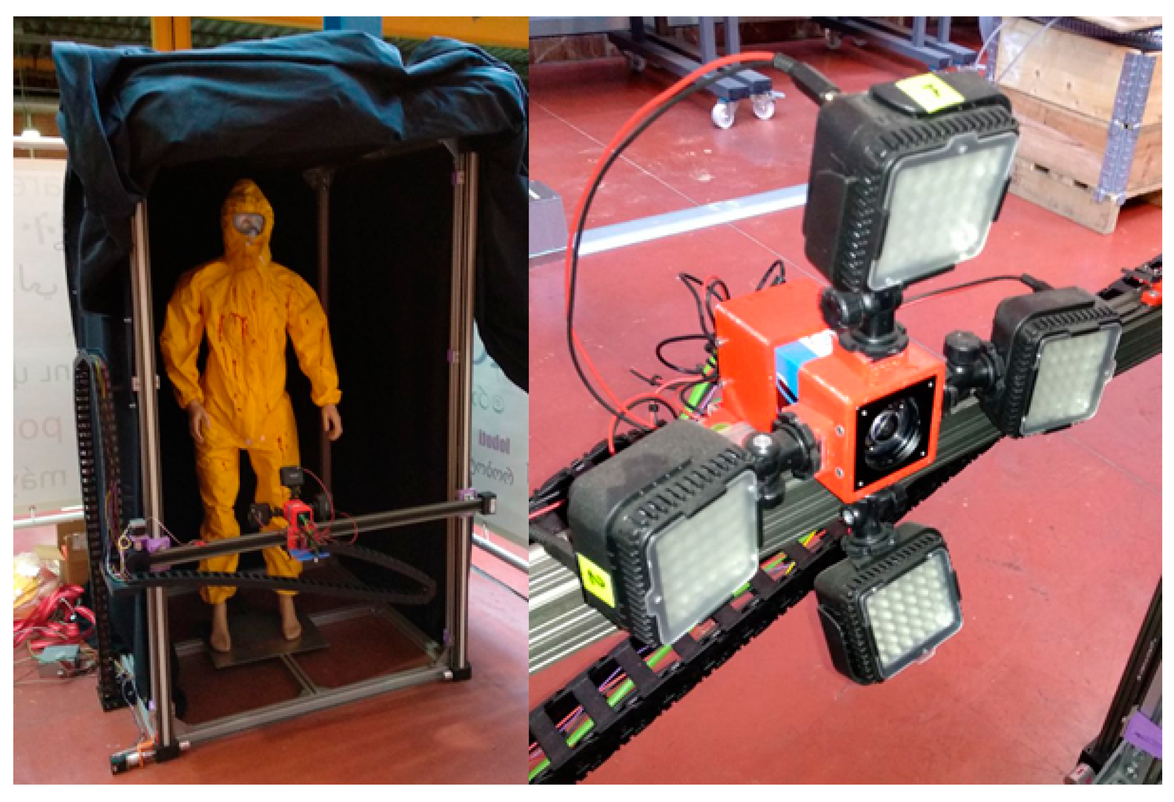
A full-body scanner prototype which resembles the systems used in airports and offices was developed between 2016 and 2019 in the University Carlos III of Madrid. These scanners are designed to detect objects under clothing and not for its surface, so the underlying technology is expensive and generally makes use of X-rays or electromagnetic radiation with complex mechanisms [14]. The HORUS full-body scanner structure was implemented in a cost-efficient way using two motors over a linear plane guidance and a camera with motorized zoom and an illumination system (Figure 1). The choice of this kind of system requires the study and use of image processing algorithms able to provide reliable data for the detection of blood traces. The study of a set of computer vision algorithms was already tested in 2019 and is one of the research areas of the project [15]. Another promising research line brings together the use of an active vision system able to detect and classify defects in PPE and the latest trends in Artificial Intelligence (AI). The current software infrastructure allows to control the robotic system manually or set an automatic scan mode that stores a set of images in predefined positions into disk. A graphical user interface was developed by the members of the project team to provide specific options to set this manual or automatic mode, as well as the possibility to adjust certain image and camera properties.
The main goal of this work is to explore and apply Reinforcement Learning (RL) to allow the current HORUS scanner platform to learn from interaction with its environment. This brings us closer to the possibility of training an AI agent for the specific blood detection task and turning it into a smarter operating system with increased reliability. The design of an agent-environment system has been simulated and evaluated considering many definitions and alternative forms of the elements of an RL problem. The effects of representational choices and the topology of the environment on the Q-Learning model-free RL algorithm are studied.
2. Materials and Methods
2.1. Learning from Interaction: Q-Learning
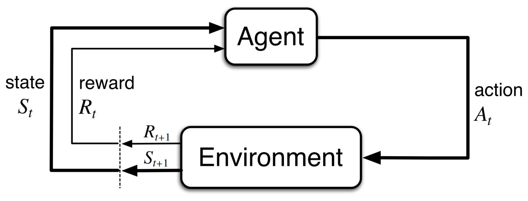
Learning from interaction is the fundamental basis of the human nature of learning, and has been computationally explored in the Reinforcement Learning (RL) field. This practice involves a learner and decision-maker agent which takes actions (A) in specific states (S) within an environment and evaluates its behavior based on some reward (R). Additional elements in RL are the policy (), a mapping that defines how the agent acts from a specific state, and a value function that determines the total amount of reward which can be accumulated over the future [16]. The mathematical formulation of this problem may be address by a Markov Decision Process (MDP) framing with finite state, action and reward sets for different discrete time steps (t, t+1…) (Figure 2). Finite MDPs formalize a sequential decision making process by defining these finite number of elements and well defined probability distributions (Equation (1)). In this equation, the definition of probability p represents the dynamics of an MDP and specifies the probability of state and reward occurring at time t, given some preceding state and action values.
These probabilities characterize the environment’s dynamics of an MPD framework able to abstract a goal-directed problem. Specifically targeting the HORUS problem, the selected algorithm was Q-Learning, a model-free RL method that finds an optimal policy by maximizing the expected value of discounted reward over a sequence of steps [17]. The value function is referred to as Q-function and allows to store subsequent Q-values, estimates of cumulative reward in the long run, in a Q-Table [16]. Q-Learning is a time-difference learning approach. This means it updates the value of a state based on the observed reward and the estimated value of the next state. It is a method based on the Bellman equation:
where Q refers to the updated Q-value for a specific state and action in a given time step t, is the step-size or learning rate, is the reward associated to the action performed, is the discount factor and is the maximum expected future reward given the new state and all the possible actions a at that new state.
2.2. OpenAI Virtual Environment
The Q-Learning algorithm will be used for the task of assisting decision making of the HORUS system. In order to simulate the environment, an open-source library and extended toolkit has been chosen. OpenAI Gym is an open source interface for developing and comparing RL algorithms, offering a way to standardize the definition of environments in AI research. In our system, Gym provided all the functionalities to test, train and simulate the blood detection task in Python code (Getting Started with Gym, available online: https://gym.openai.com/).
2.3. Problem Definition
The application of an RL algorithm to a specific problem requires to identify each element of an MDP. The MDP framework is flexible and can be referred to different problems in a wide variety of forms. Actions and states can adopt different shapes and, in general, the first ones correspond to the decisions we are interested in learning, and the second ones can be anything useful to learn these actions [16]. This may lead to the definition of the same problem in many different ways. In the HORUS definition problem, different alternative problem definitions have been considered and explored. For all of them, the robotic moving system has been treated as the agent, the actions are considered as the horizontal and vertical Cartesian movements in addition to the camera zoom, and the environment is the plane of movement inside the square-shaped security airlock covered in black flap material shown in Figure 1, as well as system parts that cannot be changed arbitrarily (such as the motors or the mechanical linkages). Besides that, two options for the definition of the state (S) have been considered:
- The first definition assumes the state (S) is the current camera position. This allows to train the system to reach some desired static position in the environment.
- The second definition encodes the state (S) depending on the content of the current camera image. This allows to avoid the static position-dependent problem derived from the first approach.
Furthermore, the design of the reward signal (R) is a crucial step of any application of RL. Modelling a reward implies deciding the scalar reward at each time step by eventually translating a goal into this signal. During training, the agent updates its policy based on this signal after some state-action combination. Therefore, the design of this value allows to drive the actions of the agent to an ideal behaviour. In practice, the design of this signal is generally performed by an informal trial and error method that evaluates if the final results are acceptable [16,18]. How shaping the reward signal affects the resulting policy will be tested.
The notion of final time step appears naturally in some problem definitions after agent-environment interactions [16]. This is the case of the HORUS problem, in which the task is done when the blood pixels are found and centered. These finite sequences of steps are referred to as episodes or epochs, and once they end the initial conditions and state are reset. The episodic task will be evaluated using 100,000 epochs.
2.4. Training Images Set
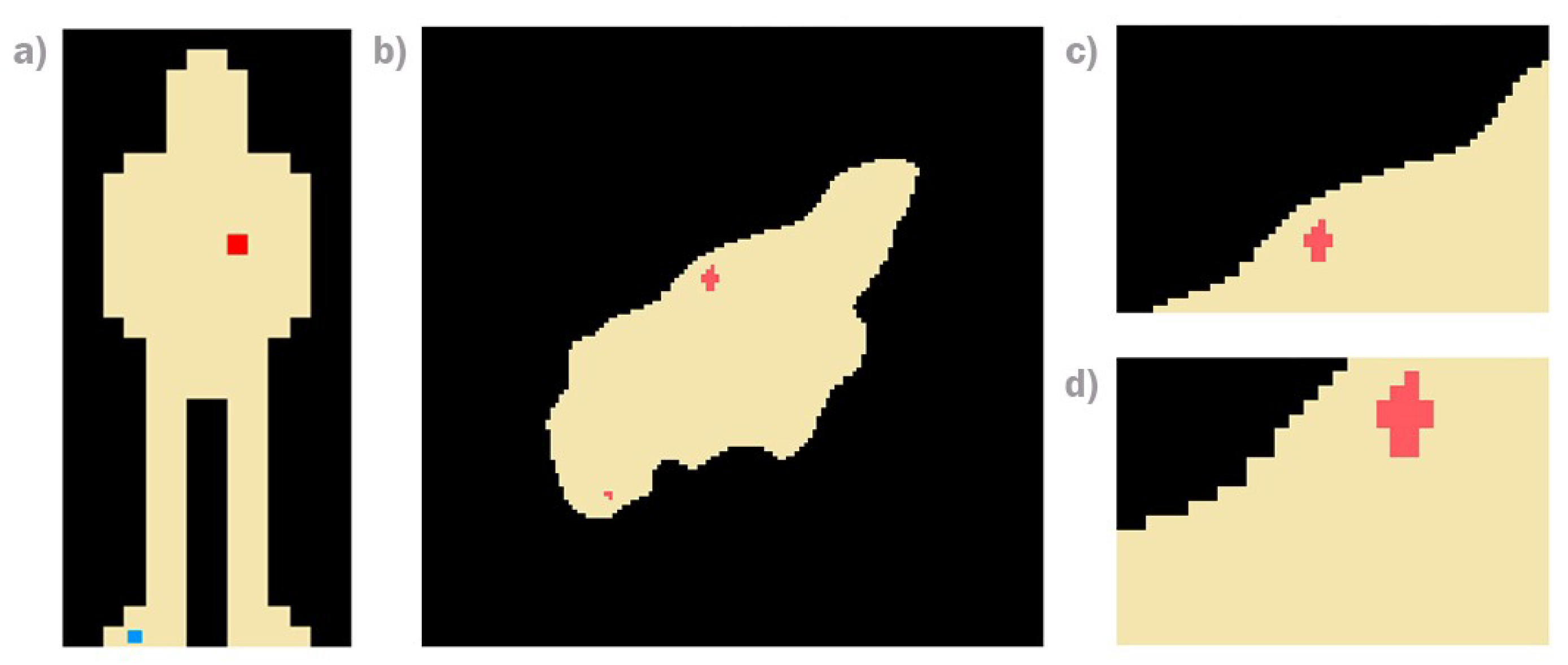
For the training of the RL active vision system, custom synthetic images have been used. This has allowed to perform all computations more efficiently and has simplified the problem to the least complex scenario. Custom images of pixels (Figure 3a) were used for the first problem definition. This set of images shows the whole visual framework of the environment, and they represent: black for the background, yellow for the medical suit and single red and blue pixels for a blood trace and the camera position, respectively. In addition, a visual framework of pixels that represent the environment (Figure 3b), where the camera is able to move and capture a window size of pixels (Figure 3c,d), has been designed. This is required because the real visual system does not allow the visualization of the entire mechanical cubicle. Every synthetic image is represented by three different pixel values identifiable with the three main elements to detect: blood (red), suit (yellow) and background (black).
2.5. Hyperparameter Tuning
Grid Search
Before presenting any results, hyperparameter optimization is applied as a final step in machine learning. Some parameters in Equation (2) are used for controlling the learning process and must be set appropriately to maximize the learning method [19]. This is the case of the learning rate and discount factor or discount rate , two parameters between 0 and 1 that evaluate how much information overwrites past information and how important are the obtained rewards compared to those obtained in further steps [20], respectively .
The learning rate or step-size parameter () affects how much the difference between a previous and a new Q-value is considered. Generally, constant small learning rates are effective in nonstationary problems in which the reward probabilities change over time. In those cases, more weight is given to recent rewards than long-past rewards. In contrast, when true values of the actions are assumed to be stationary, then the sample-average method (Equation (3)) may be used in order to average the rewards incrementally and guaranteed convergence to the true action values.
where indicates the amount of preceding selections of action a. On the whole, the step-size parameter is essential to maximize the speed of learning. Large step-sizes cause oscillations in the value function in comparison with small ones that lead to longer learning rates [21,22].
Regarding the discount rate (), it must be selected considering the time horizon of the relevant rewards for a particular action. The agent’s discounted reward as a function of the discount rate can be expressed as:
where determines the present value of future rewards. only maximizes immediate rewards and takes future rewards into account strongly. In many application it is nearly always arbitrarily chosen by researchers to be near the 0.9 point [23].
The trade-off between exploration and exploitation, one of the key challenges that arise in RL [24], is also considered at this stage. The dilemma comprises choosing between what has been learned (exploitation) or some other action to possibly increase knowledge (exploration). In general, the greedy method (that selects the action with highest learned Q-value) gets stuck performing suboptimal actions compared to the -greedy method (Equation (5)) that uses as a probability to randomly select an action, independently of action-value estimates [16]. The -greedy method follows a policy :
where is a uniform random number computed at each time step. Slightly more sophisticated strategies are Boltzmann exploration (softmax) or some derivatives of -greedy method method that reduce over time to try to get best of both high and low values [16,21].
The final step in our work will be to apply grid search to exhaustively find an optimal subset of these hyperparameters. Grid-search is used to find these optimal values of the policy which lead to the most accurate predictions [19]. For this reason, the behaviour of different agents has been evaluated according to the following metrics:
- Average number of timesteps per episode: minimum number of steps or the shortest path, is sought per episode.
- Average reward per episode: a higher number of positive rewards per episode is an indicator of an effective learning.
- Reward/Timesteps ratio: a higher value of this ratio enables to get the maximum reward as fast as possible.
3. Results
3.1. State Space: Absolute Camera Coordinates (Path Learner)
Each approach in this study implied the implementation of a Gym environment to test it. The first idea to explore was a system able to guide the agent to specific locations. Similar to computer programs capable of imitating or exceeding human-level performance on many games through RL and variants of this learning method [25] such as Pacman [26], actions performed by the agent in the proposed system were rewarded according to the following criteria.
3.1.1. State and Action Space
- The discrete world to explore is a grid where the state is defined by the position of the camera in one of these locations.
- The number of possible states is therefore .
- The set of possible actions A is the same for all states , .
3.1.2. Reward Shaping
- The main target is met when the camera location (blue pixel) reaches the blood trace (red pixel).
- Reaching the goal yields +100 positive reward and stops the episode.
- Illegal background location yields −100 penalty points and stops the episode.
- A −1 negative reward results after each performed action except for MU and MD movements that was a −2 reward. This strategy allows to encourage the agent to perform the fewest number of possible moves to reach the goal and to promote some actions over others (x-axis over y-axis movements).
- The system takes into account some nonstationary considerations such as real patients movements. For this purpose the blood sample (red pixel) moves randomly given some small probability.
3.1.3. Performance
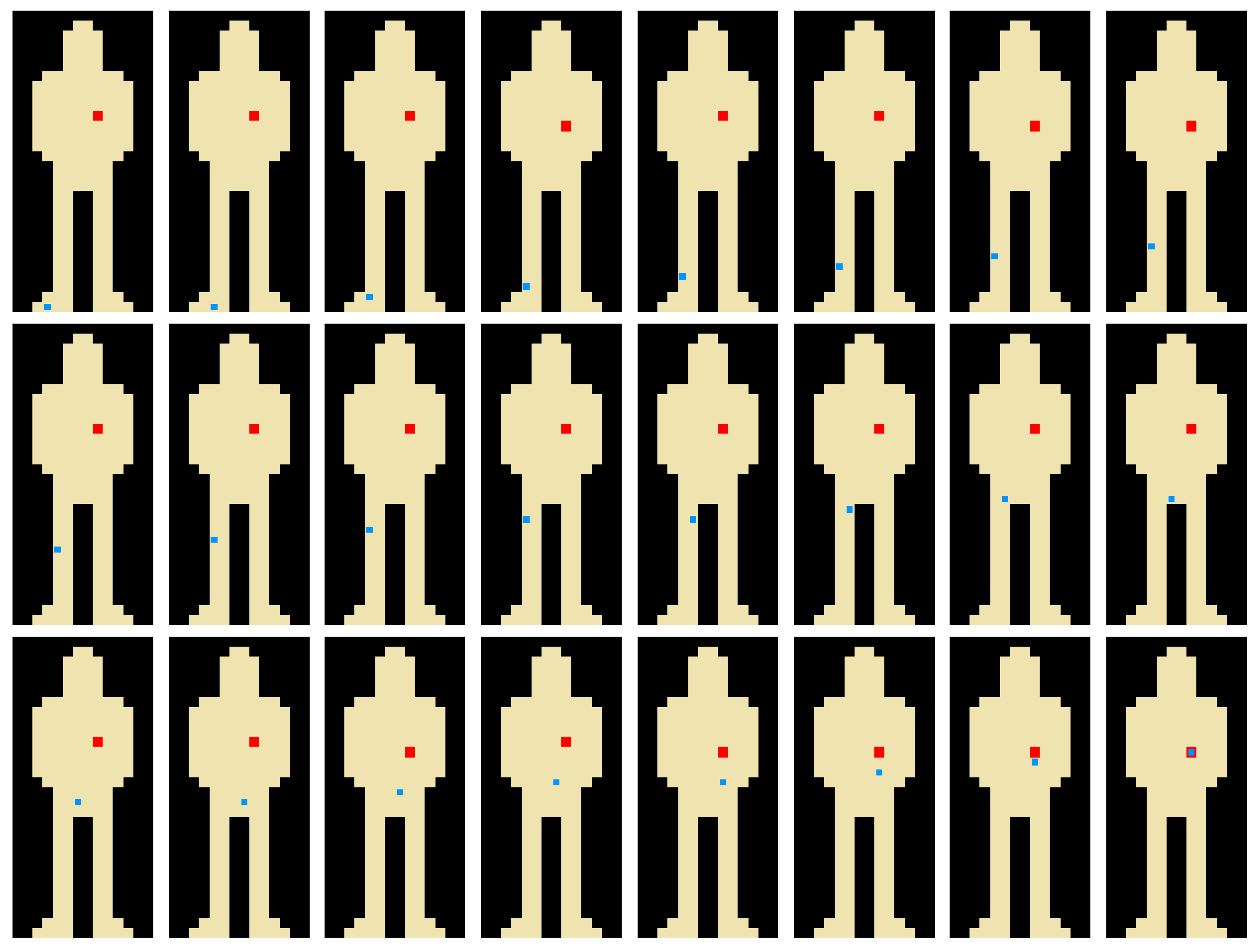
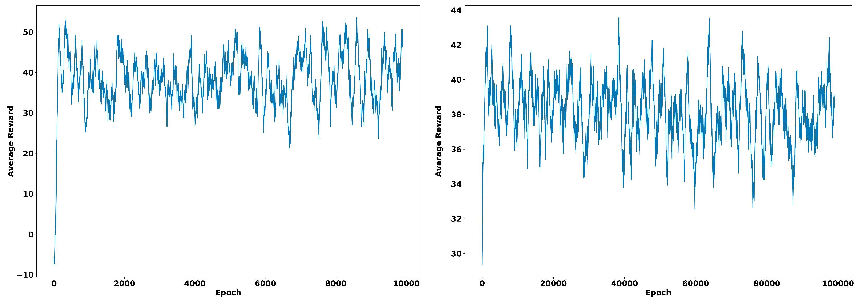
An example of 10,000 episodes (starting from the same initial camera state) is shown in Figure 4. Exploration, learning rate and discount factor were fixed values (0.1, 0.1 and 0.6, respectively). The agent behaviour reached the goal in 24 steps (represented in the images as different states) with an overall average reward of −6.1 units. Average reward through time is shown in Figure 5 (left) for the different training episodes. Increasing the number of episodes 10 times, gives a whole average reward of −2.9 units. The average reward progress in this case is represented in Figure 5 (right).
Nevertheless, testing any of these trained Q-Tables by using a different framework (moving several pixels the blood sample) leads to inefficient results. The agent only knows how to move greedily to a specific location area and it fails to reach the goal in any other cases. This approach is a goal-dependent learning method.
3.2. Space State: Blood Spot Coordinates in the Camera View
The second definition was framed with the intention of overcoming this goal-dependent limitation. The chief change in this respect was identifying a new decision making task by updating the meaning of state. For this purpose, a new criteria was established.
3.2.1. State and Action Space
- The discrete world to explore is an grid where the state is defined by the position of the blood sample in one of these locations that corresponds to the pixels of the camera view. These positions are encoded in the OpenAI environment into a sequence of consecutive states.
- Blood samples can be represented by more than 1 pixel as shown in the different camera views in Figure 3. The final state is given after computing the center of mass of the blood sample.
- Two level zooms with the same pixel resolution ( pixels) were considered to simulate the real 3D problem. Zoom Out images with pixels are down-sampled to reduce the dimensionality using nearest-neighbor interpolation.
- The number of possible states raises up to . This number takes into account both levels of zooms and the null case (no blood appears in the image).
- Big [b] and small [s] steps of 4 and 1 pixel, respectively, in Move Left (ML), Move Right (MR), Move Up (MU) and Move Down (MD) actions are considered, as well as Zoom Out (ZO) and Zoom In (ZI)) movements. The set of possible actions A varies for each state , .
- Invalid joints space actions such as trying ZI action when the current state in already in this framework, are not included as possible movements in the action space
3.2.2. Reward Shaping I
- If some blood pixels appear in the camera view, the reward is proportional to the area of red pixels (favouring ZI states) and inversely proportional to the squared distance to the central position.
- The main target is met when the centroid of blood pixels is centered in the ZI camera view.
- Reaching the goal yields +1000 positive reward and stops the episode.
- Each step is penalized by a −50 negative reward to avoid unnecessary movements from the agent.
3.2.3. Reward Shaping II
- If some blood pixels appear in the camera view, the reward is proportional to the area of red pixels (favouring ZI states).
- Getting closer to the centroid position respect to previous state yields a +10 positive reward.
- Moving away from the centroid position respect to previous state yields a −20 negative reward.
- The main target is met when the centroid of blood pixels is centered in the ZI camera view.
- Reaching the goal yields +1000 positive reward and stops the episode.
3.2.4. Grid Search
Learning rate (), discount factor () and exploration () hyperparameters are external values to the model and cannot be estimated from data. These values have to be set before the learning process begins. These analysis have been conducted using the two already described reward shaping definitions.
The overall performance of eight different agents with a combination of these hyperparameters is shown in Table 1. Results represent the average of five different trainings for each hyperparameters combination using a reward shaping inversely proportional to the centroid distance that penalizes each performed step (Reward Shaping I).
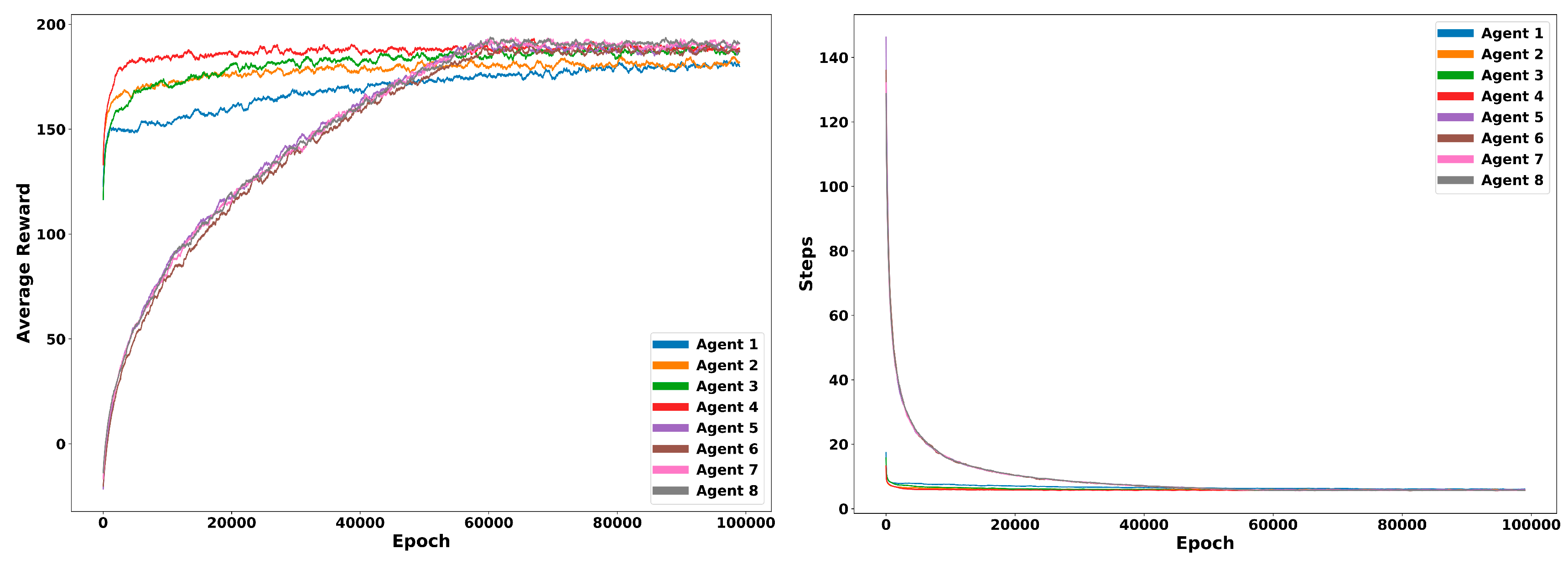
In addition, performance over time is analyzed to compare how each combination of hyperparameters behaves. Total average reward of each episode is compared for each agent in Figure 6 together with the average number of steps performed. Average results corresponds to five different trainings for each combination of hyperparameters.
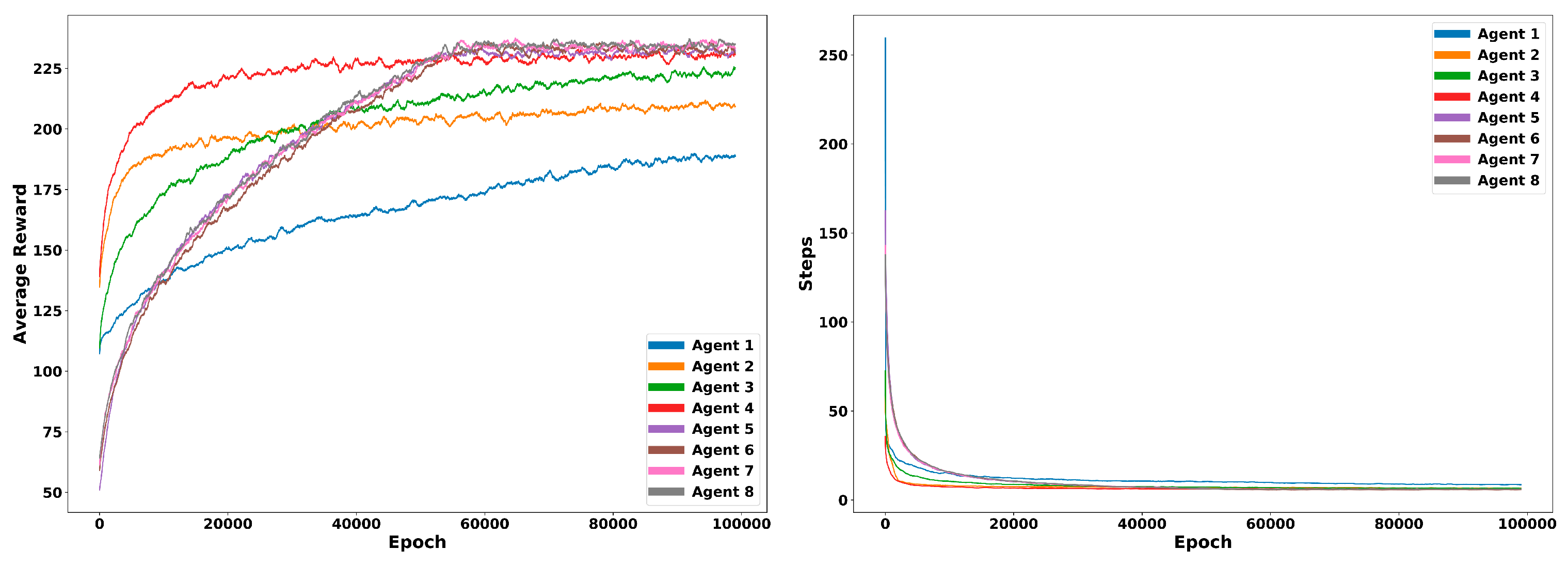
The same experiment was performed using a different distribution of rewards (Reward Shaping II). The overall performance of the same eight agents is summarized in Table 2. Performance over time is also plot for each combination of hyperparameters. The same amount of runs and conditions are used for showing the average reward and the number of steps along time in Figure 7.
3.2.5. Performance
Training the agent under these principles was carried out by selecting random initial camera view frames. First results suggested the system would get stuck if the random initial camera view frames were far away from any blood sample. Chaotic movements were observed under the null case state, but the system learned to reach the target if the initial frame captured any blood spot. This is likely an exploration issue where the agent is unable to find the exit the first time. The reformulation of the problem by a possible combination of this AI approach with the automatic scan mode of the HORUS scanner was considered at this stage.
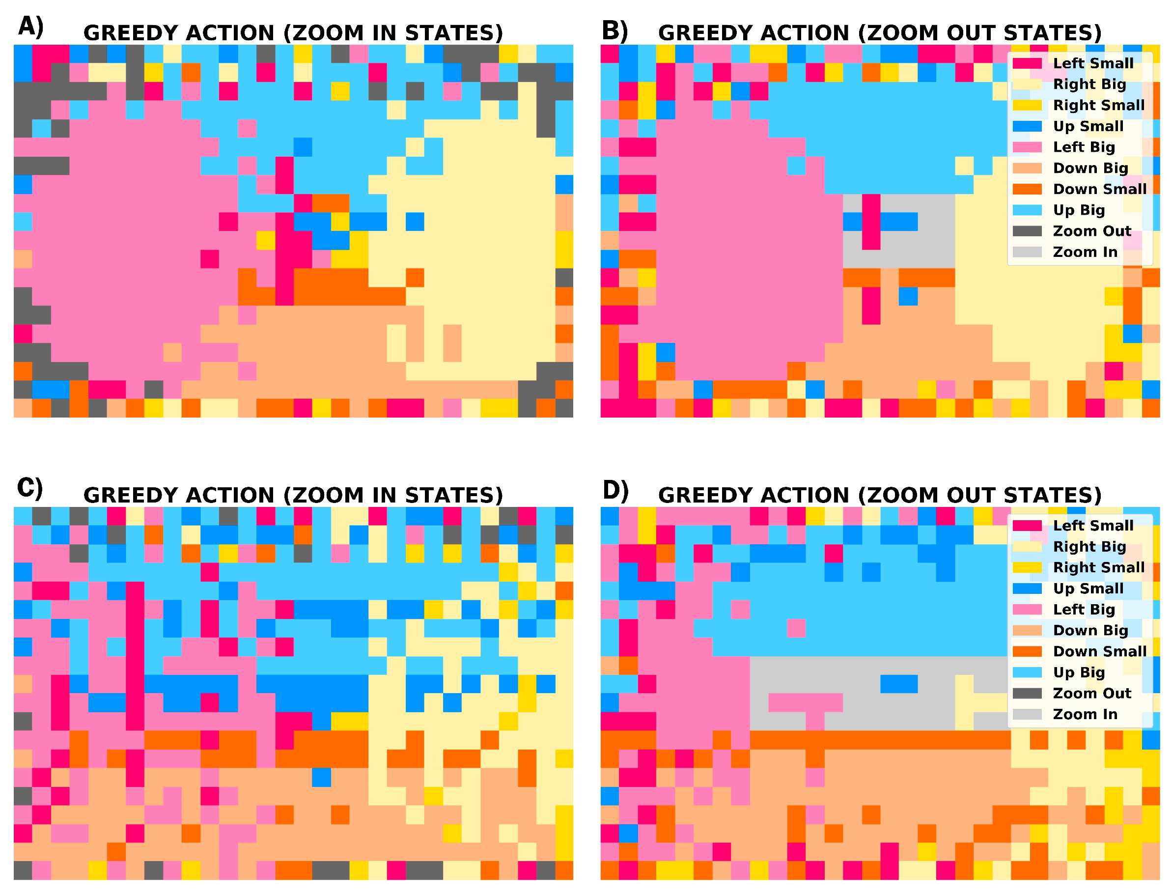
An example of training of 100,000 episodes (starting from random initial frames capturing any blood pixel) is shown in Figure 8. Exploration, learning rate and discount factor were the values for Agent 8 in previous experiments. A and B images represent the result for the first definition of rewards for ZI and ZO states, respectively, in contrast to C (ZI) and D (ZO) that correspond to the second reward shaping. The action with highest Q-Value is represented by a different color and those actions are the Cartesian movements of the camera image views respect to the whole image framework. No invalid joint space actions are observed in the images.
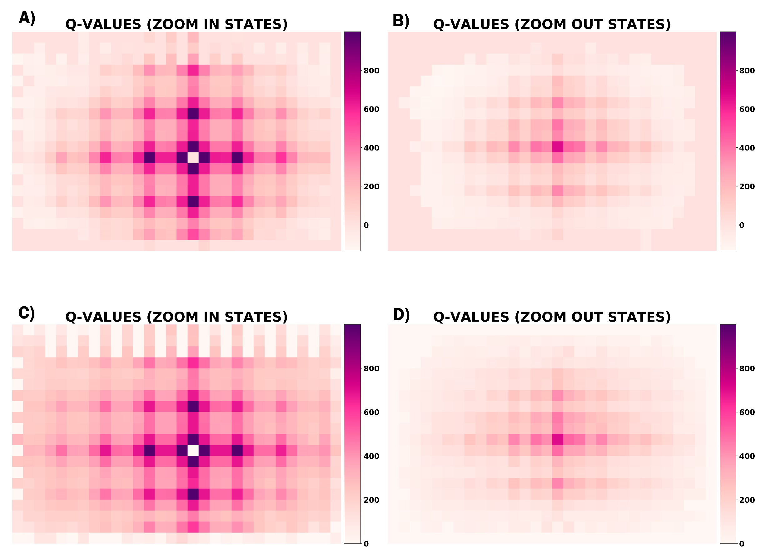
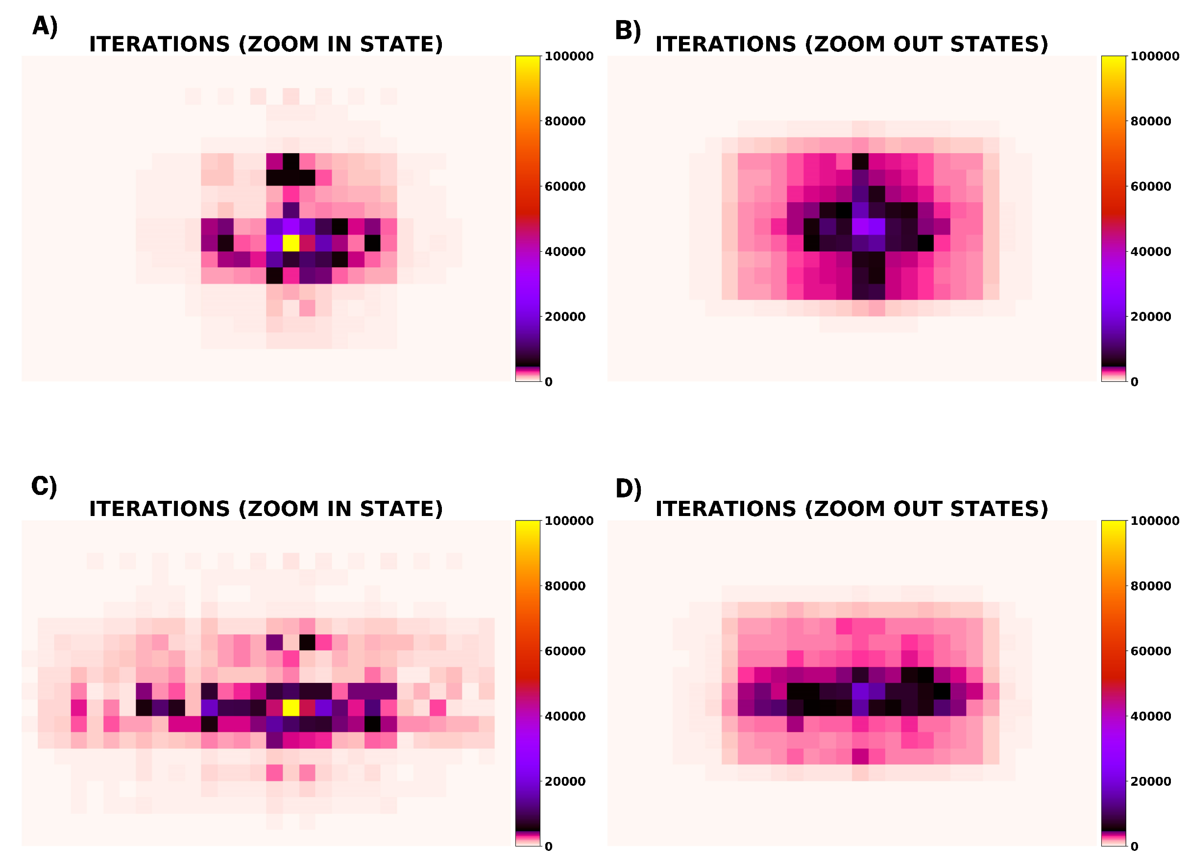
In order to quantify how reliable the indicated greedy actions are, Figure 9 and Figure 10 represent the Q-Values of greedy actions, a measure of goodness for a iteratively updated state-action pair [27], and a counter of how many times the agent has come through each state during the whole training, respectively.
4. Discussion
Reinforcement learning is considered to be the third machine learning paradigm, along with supervised and unsupervised learning [28]. The modern field of RL was preceded by two independent focus of interest: learning by trial and error in the psychology field and the design of controllers to adjust some dynamical system’s measure over time [16]. The early history of RL justifies the selection of this technique for developing an adaptive control system able to learn from its own experience and behaviour. Added values such as the possibility of using offline computation [29] or the possibility of applying this method to changing environments [30], support the choice. In particular, Q-Learning is the most popular and it is thought to be the most effective model-free algorithm. This architecture converges to the optimal values as long as state-action pairs are tried enough and learning proceeds similarly to other temporal difference methods [17,28].
The design of a representation of the HORUS problem led the process of evaluation of different alternatives. Based on the fact that actions and states vary from task to task and their shape affects the system performance, the choice of a specific model greatly impacts final results. The first considered option has been a system able to navigate to a specific location in the proposed environment. In practice, the system worked correctly and found the predefined goal when testing. Nevertheless, moving the goal caused the system to fail, because the previously learned information interferes with the task of finding the new goal. Although the Q-learning algorithm is independent of the policy being followed, it was shown that is not independent of the current goal. Concurrent RL has been studied in many applications to learn the relative proximity of all the states simultaneously and apply RL for dynamic goals and environments [31]. This method address the problem through specific algorithms that use a temporal difference approach able to learn a mapping and to allow coordinate learning in a goal independent way.
In this work, another strand of research assessed this problem by changing the identification of state. Defining the RL element of state by the pixel position of a blood sample (or its center of mass) instead of the position coordinates of the camera, eliminate the goal dependant problem. However, the behaviour of the system under no presence of blood samples is difficult to adjust and generally the experiments showed that the system would get lost. The considered approach for the real problem involves the use of a semi-automatic inspection able to move and visualize all the cubicles in the search of blood traces and to center and magnify the image at the presence of any sample.
The selection of rewards is in first instance an arbitrary process and the choice must be decided given that the agent always learns to maximize them. Thus, it is crucial that the rewards we set up truly indicate what we want to accomplish. Reward measures could be specified either continuous or discrete signals and are designed to avoid sparse or under-specified rewards [16]. Two different discrete reward structures were investigated. In either case, reward signals provided rich information when the action and observation signals change. In the first consideration, the signal penalized each step to avoid unnecessary movements and the reward was proportional to the distance to the center. In the second design, getting close to the center compared to last state gave positive reward and getting away yielded a negative reward.
Efficiency was analysed for each of the reward designs and for a group of 8 agents. Figure 6 and Figure 7 show the performance in terms of average reward of these agents. Although, Reward/TimeStep ratio (Table 1 and Table 2) is in general better for Agents 1–4, plotting the results over time show that final reward improves in Agents 5–8 due to the use of an epsilon decaying method to regulate exploration. Exploration is needed because there is always uncertainty about the accuracy of the action-value estimates. From the several simple ways to balancing exploration and exploitation that have been used in this work, it seems that -decay approach achieves better results than the rest. This method reduces the exploration hyperparamer in each iteration, allowing to explore more state-action pairs at the beginning of training and eventually reducing the number of non-greedy movements.
Among the rest of hyperparameters, best average reward and reduced timesteps are found using the averaging method (1/N) for stationary problems in comparison with a constant step-size parameter generally applied for nonstationary cases. In addition, the discount factor of 0.6 units reported the best results in all the experiments performed (Table 1 and Table 2).
In Figure 8 the circular pattern around the center of the images indicate that Agent 8 learns to center the centroid of the blood trace in both zoom states. Comparing both greedy behaviours, Reward Shaping I appears to be the most effective to center the blood sample because regions are defined more sharply and less random movements are noticed. Looking at Figure 9 and Figure 10, higher Q-Values and steps are observed in the regions with high rates of visits. Edge locations are less frequent and consequently the greedy behaviour in these zones is greatly randomized.
A future research direction implies extracting the reward signal by using Inverse Reinforcement Learning (IRL). This mechanism allows to extract the rewards and use them to learn a policy, assuming knowledge of the environment’s dynamics [16]. Because the boundary of the Reinforcement Learning field is based on the implicit assumption that the reward function is the most robust definition of the task, learning that function is a reasonable approach to consider [32].
The implementation of a simple simulated environment leaves aside the real behaviour of the system. Complex considerations derived from the real world experience such as the appearance of two blood samples, other kind of detectable fluids that may appear in the camera view or sudden movements of the health-provider have not be taken into account. In addition, the resolution of real images is larger than the one used for this analysis, as well as the complexity in RGB colors. In another line of action, Deep Reinforcement Learning, may help to the task of adapting the simulation to the real system. Training deep neural networks just like recent improvements in computer vision [25] and connect the idea to RL to operate on RGB images and process training data may be a promising task.
The recent outbreak of 2019 novel coronavirus diseases (COVID-19) in Wuhan, China has awakened the need to increase infection control capacity to prevent transmission in health care settings [33]. The advantages at social level that may arise from this project include increasing the safety of the facilities and workers in medical environments, the replication of this technology in other areas of the hospital (intensive care units, operating theatres…), special aid in the detection of contaminants and germs related to new and highly contagious diseases, and the discovery of additional lines of research. For instance, other possible application types include active vision control for surveillance purposes, such as mobile exploring robots that perform visual inspection of historical places and objects [34], navigation tasks in different environments or guiding motions of robotic manipulators [35].
5. Conclusions
An AI agent able to center blood samples has been designed through Reinforcement Learning. Representational choices such as reward shaping or the general adjustment of a custom problem to an MDP framework is a crucial issue to address, although resolutions are at present more art than science [16]. Trial and error formulas worked for the specific problem. Hyperparameter optimization helped determine the best combination of these values and should be tested for each application. The learning rate set up for stationary cases using the sample-average method, as well as a specific epsilon decaying method worked best for the trained agents. A prototype of an active vision system has been designed through Q-Learning in a simulation environment.
Author Contributions
Conceptualization, A.G.R. and J.G.V.; Methodology, A.G.R. and J.G.V.; Software, A.G.R. and B.Ł.; Validation, J.G.V. and C.B.; Formal analysis, J.G.V.; Investigation, A.G.R. and J.G.V.; Resources, C.B.; Data Curation, A.G.R.; Writing–original draft preparation, A.G.R.; Writing–review and editing, J.G.V. and C.B.; Visualization, J.G.V.; Supervision, J.G.V. and C.B.; Project administration, J.G.V. and C.B.; Funding acquisition, C.B. All authors have read and agreed to the published version of the manuscript.
Funding
The research leading to these results received funding from: Inspección robotizada de los trajes de proteccion del personal sanitario de pacientes en aislamiento de alto nivel, incluido el ébola, Programa Explora Ciencia, Ministerio de Ciencia, Innovación y Universidades (DPI2015-72015-EXP); the RoboCity2030-DIH-CM Madrid Robotics Digital Innovation Hub (“Robótica aplicada a la mejora de la calidad de vida de los ciudadanos. fase IV”; S2018/NMT-4331), funded by “Programas de Actividades I+D en la Comunidad de Madrid” and cofunded by Structural Funds of the EU; and ROBOESPAS: Active rehabilitation of patients with upper limb spasticity using collaborative robots, Ministerio de Economía, Industria y Competitividad, Programa Estatal de I+D+i Orientada a los Retos de la Sociedad (DPI2017-87562-C2-1-R).
Conflicts of Interest
The authors declare no conflict of interest.
Abbreviations
The following abbreviations are used in this manuscript:
| EHF | Ebola Hemorrhagic Fever |
| MHF | Marburg Hemorrhagic Fever |
| HID | Highly Infectious Diseases |
| HLIU | High-Level Isolation Units |
| PPE | Personal Protective Equipment |
| IPC | Infection Prevention and Control |
| WHO | World Health Organization |
| AI | Artificial Intelligence |
| RL | Reinforcement Learning |
| MDP | Markov Decision Process |
| ML | Move Left |
| MR | Move Right |
| MU | Move Up |
| MD | Move Down |
| ZO | Zoom Out |
| ZI | Zoom In |
References
- MacNeil, A.; Rollin, P.E. Ebola and marburg hemorrhagic fevers: Neglected tropical diseases? PLoS Negl. Trop. Dis. 2012, 6, E1546. [Google Scholar] [CrossRef] [PubMed] [Green Version]
- World Health Organization. Estimating Mortality from COVID-19. 2020. Available online: https://www.who.int/publications/i/item/WHO-2019-nCoV-Sci-Brief-Mortality-2020.1 (accessed on 26 August 2020).
- Schilling, S.; Fusco, F.M.; De Iaco, G.; Bannister, B.; Maltezou, H.C.; Carson, G.; Gottschalk, R.; Brodt, H.-R.; Brouqui, P.; Puro, V.; et al. Isolation facilities for highly infectious diseases in Europe—A cross-sectional analysis in 16 countries. PLoS ONE 2014, 9, e100401. [Google Scholar] [CrossRef]
- Fusco, F.M.; Brouqui, P.; Ippolito, G.; Vetter, N.; Kojouharova, M.; Parmakova, K.; Skinhoej, P.; Siikamaki, H.; Perronne, C.; Schilling, S.; et al. Highly infectious diseases in the Mediterranean Sea area: Inventory of isolation capabilities and recommendations for appropriate isolation. New Microbes New Infect. 2018, 26, S65–S73. [Google Scholar] [CrossRef] [PubMed]
- Herstein, J.J.; Biddinger, P.D.; Gibbs, S.G.; Le, A.B.; Jelden, K.C.; Hewlett, A.L.; Lowe, J.J. High-Level Isolation Unit Infection Control Procedures. Health Secur. 2017, 15, 519–526. [Google Scholar] [CrossRef] [PubMed]
- Sykes, A. An International Review Of High Level Isolation Units. WCMT Report Document. 2019. Available online: https://www.wcmt.org.uk/sites/default/files/report-documents/Sykes%20A%202018%20Final_0.pdf (accessed on 26 August 2020).
- WHO Ebola Response Team. After Ebola in West Africa—Unpredictable Risks , Preventable Epidemics. N. Engl. J. Med. 2016, 375, 587–596. [Google Scholar] [CrossRef] [PubMed]
- Subprograma Estatal de Generación de Conocimiento | Programa Estatal de Fomento de la Investigación Científica y Técnica de Excelencia | Plan Estatal de Investigación Científica y Técnica y de Innovación 2013–2016 | Convocatorias—Ministerio de Ciencia, Innovación y Universidades (es). Available online: http://www.ciencia.gob.es/portal/site/MICINN/menuitem.dbc68b34d11ccbd5d52ffeb801432ea0/?vgnextoid=042e9db3abf1e410VgnVCM1000001d04140aRCRD (accessed on 26 August 2020).
- HORUS | Robotics Lab—Where Technology Happens. Available online: http://roboticslab.uc3m.es/roboticslab/project/horus (accessed on 26 August 2020).
- Michael, K. Coronavirus disease 2019 (COVID-19): Protecting hospitals from the invisible. Ann. Intern. Med. 2020, 127, 619–620. [Google Scholar]
- World Health Organization. Personal Protective Equipment for Use in a Filovirus Disease Outbreak Rapid Advice Guideline; WHO Guidelines; World Health Organization: Geneva, Switzerland, 2016; Available online: https://www.who.int/csr/resources/publications/ebola/personal-protective-equipment/en/ (accessed on 26 August 2020).
- World Health Organization. How to Put on and How to Remove Personal Protective Equipment—Posters. 2015. Available online: https://www.who.int/csr/resources/publications/ebola/ppe-steps/en/ (accessed on 26 August 2020).
- Grandbastien, B.; Parneix, P.; Berthelot, P. Putting on and removing personal protective equipment. N. Engl. J. Med. 2015, 372, E16. [Google Scholar]
- Bello-Salau, H.; Salami, A.F.; Hussaini, M. Ethical analysis of the full-body scanner (FBS) for airport security. Adv. Nat. Appl. Sci. 2012, 6, 664–672. [Google Scholar]
- Stazio, A.; Victores, J.G.; Estevez, D.; Balaguer, C. A Study on Machine Vision Techniques for the Inspection of Health Personnels’ Protective Suits for the Treatment of Patients in Extreme Isolation. Electronics 2019, 8, 743. [Google Scholar] [CrossRef] [Green Version]
- Sutton, R.S.; Barto, A.G. Reinforcement Learning: An Introduction; MIT Press: Cambridge, MA, USA, 1998. [Google Scholar]
- Watkins, C.J.C.H.; Dayan, P. Q-Learning. Mach. Learn. 1992, 8, 279–292. [Google Scholar] [CrossRef]
- Andrew, Y.N.; Harada, D.; Russell, S. Policy invariance under reward transformations: Theory and application to reward shaping. In Proceedings of the Sixteenth International Conference on Machine Learning, Bled, Slovenia, 27–30 June 1999. [Google Scholar]
- Claesen, M.; De Moor, B. Hyperparameter Search in Machine Learning. arXiv 2015, arXiv:1502.02127. [Google Scholar]
- Eyal, E.; Yishay, M. Learning Rates for Q-learning Eyal Even-Dar Yishay Mansour. J. Mach. Learn. Res. 2003, 5, 1–25. [Google Scholar]
- Tokic, M. Adaptive ϵ-greedy exploration in reinforcement learning based on value differences. In Proceedings of the 33rd Annual German Conference on Advances in Artificial Intelligence, Karlsruhe, Germany, 21–24 September 2010. [Google Scholar]
- George, A.P.; Powell, W.B. Adaptive stepsizes for recursive estimation with applications in approximate dynamic programming. Mach. Learn. 2006, 65, 167–198. [Google Scholar] [CrossRef] [Green Version]
- François-Lavet, V.; Fonteneau, R.; Ernst, D. How to discount deep reinforcement learning: Towards new dynamic strategies. arXiv 2015, arXiv:1512.02011. [Google Scholar]
- Dos Santos Mignon, A.; De Azevedo Da Rocha, R.L. An Adaptive Implementation of ϵ-Greedy in Reinforcement Learning. Procedia Comput. Sci. 2017, 109, 1146–1151. [Google Scholar] [CrossRef]
- Mnih, V.; Kavukcuoglu, K.; Silver, D.; Graves, A.; Antonoglou, I.; Wierstra, D.; Riedmiller, M. Playing Atari with Deep Reinforcement Learning. arXiv 2013, arXiv:1312.5602. [Google Scholar]
- Rohlfshagen, P.; Liu, J.; Perez-Liebana, D.; Lucas, S.M. Pac-Man Conquers Academia: Two Decades of Research Using a Classic Arcade Game. IEEE Trans. Games 2017, 10, 233–256. [Google Scholar] [CrossRef]
- Zap, A.; Joppen, T.; Fürnkranz, J. Deep Ordinal Reinforcement Learning. arXiv 2019, arXiv:1905.02005. [Google Scholar]
- Kaelbling, L.P.; Littman, M.L.; Moore, A.W. Reinforcement Learning: A Survey. J. Artif. Intell. Res. 1996, 4, 237–285. [Google Scholar] [CrossRef] [Green Version]
- Mandel, T.; Liu, Y.; Brunskill, E.; Popovic, Z. Offline evaluation of online reinforcement learning algorithms. In Proceedings of the 30th Conference on Artificial Intelligence, Phoenix, AZ, USA, 12–17 February 2016. [Google Scholar]
- Lane, T.; Ridens, M.; Stevens, S. Reinforcement learning in nonstationary environment navigation tasks. Adv. Artif. Intell. 2007, 429–440. [Google Scholar]
- Ollington, R.B.; Vamplew, P.W. Concurrent Q-learning: Reinforcement learning for dynamic goals and environments. Int. J. Intell. Syst. 2005, 20, 1037–1052. [Google Scholar] [CrossRef]
- Abbeel, P.; Ng, A.Y. Apprenticeship learning via inverse reinforcement learning. In Proceedings of the Twenty-First International Conference on Machine Learning, Banff, AB, Canada, 4–8 July 2004; pp. 1–8. [Google Scholar]
- Wang, C.; Horby, P.W.; Hayden, F.G.; Gao, G.F. A novel coronavirus outbreak of global health concern. Lancet 2020, 395, 470–473. [Google Scholar] [CrossRef] [Green Version]
- Ceccarelli, M.; Cafolla, D.; Carbone, G.; Russo, M.; Cigola, M.; Senatore, L.J.; Gallozzi, A.; Di Maccio, R.; Ferrante, F.; Bolici, F.; et al. HeritageBot service robot assisting in cultural heritage. In Proceedings of the 2017 First IEEE International Conference on Robotic Computing (IRC), Taichung, Taiwan, 10–12 April 2017. [Google Scholar]
- Chen, S.; Li, Y.; Kwok, N.M. Active vision in robotic systems: A survey of recent developments. Int. J. Robot. Res. 2011, 30, 1343–1377. [Google Scholar] [CrossRef]
Figure 1.
HORUS full-body scanner structure: (left) Overall mechanism view and (right) illumination system composed of a motorized camera DFK Z12G445 and 4 Neewer CN-Lux260 lamps.
Figure 1.
HORUS full-body scanner structure: (left) Overall mechanism view and (right) illumination system composed of a motorized camera DFK Z12G445 and 4 Neewer CN-Lux260 lamps.

Figure 2.
Block diagram of the Agent-Environment interaction in a Markov Decision Process [16].
Figure 2.
Block diagram of the Agent-Environment interaction in a Markov Decision Process [16].

Figure 3.
Example of synthetic images of four different RGB colors (Black, Yellow, Red and Blue) that simulate the background, medical suit, blood traces and camera position of the HORUS problem, respectively. Emulates: (a) least zoom, (b,c) intermediate zoom, (d) maximum zoom.
Figure 3.
Example of synthetic images of four different RGB colors (Black, Yellow, Red and Blue) that simulate the background, medical suit, blood traces and camera position of the HORUS problem, respectively. Emulates: (a) least zoom, (b,c) intermediate zoom, (d) maximum zoom.

Figure 4.
Example of behaviour after 10,000 epochs for training a camera agent (blue pixel) to reach a specific location (blood pixel) through Q-Learning. First state corresponds to upper left image and increases to the right.
Figure 4.
Example of behaviour after 10,000 epochs for training a camera agent (blue pixel) to reach a specific location (blood pixel) through Q-Learning. First state corresponds to upper left image and increases to the right.

Figure 5.
Average reward after (left) 10,000 epochs and (right) 100,000 epochs training of a camera agent to reach a specific location through Q-Learning.
Figure 5.
Average reward after (left) 10,000 epochs and (right) 100,000 epochs training of a camera agent to reach a specific location through Q-Learning.

Figure 6.
Total reward on episode averaged over 5 different runs for eight different agents (left) and the total number of steps averaged over these runs (right) using Reward Shaping I. The training of each agent comprised 100,000 episodes and curves are smoothed with a window of 1000 epochs.
Figure 6.
Total reward on episode averaged over 5 different runs for eight different agents (left) and the total number of steps averaged over these runs (right) using Reward Shaping I. The training of each agent comprised 100,000 episodes and curves are smoothed with a window of 1000 epochs.

Figure 7.
Total reward on episode averaged over 5 different runs for eight different agents (left) and the total number of steps averaged over these runs (right) using Reward Shaping II. The training of each agent comprised 100,000 episodes and curves are smoothed with a window of 1000 epochs.
Figure 7.
Total reward on episode averaged over 5 different runs for eight different agents (left) and the total number of steps averaged over these runs (right) using Reward Shaping II. The training of each agent comprised 100,000 episodes and curves are smoothed with a window of 1000 epochs.

Figure 8.
Example of greedy behaviour after 100,000 epochs for training a camera agent to center a blood spot through Q-Learning. The state is a different camera view of the blood trace and the ten possible actions (represented by colors) are movements of the camera respect to the whole image framework. (A) (ZI) and (B) (ZO) images corresponds to Agent 8 (Reward Shaping I) and (C) (ZI) and (D) (ZO) images are for Agent 8 (Reward Shaping II).

Figure 9.
Q-Values of greedy actions for each state in the two possible Zoom configurations after 100,000 training epochs. (A) (ZI) and (B) (ZO) images corresponds to Agent 8 (Reward Shaping I) and (C) (ZI) and (D) (ZO) images are for Agent 8 (Reward Shaping II).
Figure 9.
Q-Values of greedy actions for each state in the two possible Zoom configurations after 100,000 training epochs. (A) (ZI) and (B) (ZO) images corresponds to Agent 8 (Reward Shaping I) and (C) (ZI) and (D) (ZO) images are for Agent 8 (Reward Shaping II).

Figure 10.
Iteration values representing how many times each state has been visited during 100,000 training epochs. (A) (ZI) and (B) (ZO) images corresponds to Agent 8 (Reward Shaping I) and (C) (ZI) and (D) (ZO) images are for Agent 8 (Reward Shaping II).
Figure 10.
Iteration values representing how many times each state has been visited during 100,000 training epochs. (A) (ZI) and (B) (ZO) images corresponds to Agent 8 (Reward Shaping I) and (C) (ZI) and (D) (ZO) images are for Agent 8 (Reward Shaping II).


Table 1.
Performance of 8 agents with different hyperparameter values, after 100,000 epochs training using Reward Shaping I.
Table 1.
Performance of 8 agents with different hyperparameter values, after 100,000 epochs training using Reward Shaping I.
| Agent 1 | Agent 2 | Agent 3 | Agent 4 | Agent 5 | Agent 6 | Agent 7 | Agent 8 | |
|---|---|---|---|---|---|---|---|---|
| Learning Rate () | 0.1 | 1/N | 0.1 | 1/N | 0.1 | 1/N | 0.1 | 1/N |
| Discount Factor () | 0.9 | 0.9 | 0.6 | 0.6 | 0.9 | 0.9 | 0.6 | 0.6 |
| Exploration () | 0.1 | 0.1 | 0.1 | 0.1 | -decay | -decay | -decay | -decay |
| Average Reward per episode | 170 | 177 | 181 | 187 | 154 | 151 | 154 | 154 |
| Average Timesteps per episode | 7 | 6 | 6 | 6 | 11 | 10 | 10 | 10 |
| Rewards/Timesteps ratio | 25 | 29 | 30 | 32 | 15 | 15 | 15 | 15 |
Table 2.
Performance of 8 agents with different hyperparameter values after 100,000 epochs training using Reward shaping II.
Table 2.
Performance of 8 agents with different hyperparameter values after 100,000 epochs training using Reward shaping II.
| Agent 1 | Agent 2 | Agent 3 | Agent 4 | Agent 5 | Agent 6 | Agent 7 | Agent 8 | |
|---|---|---|---|---|---|---|---|---|
| Learning Rate () | 0.1 | 1/N | 0.1 | 1/N | 0.1 | 1/N | 0.1 | 1/N |
| Discount Factor () | 0.9 | 0.9 | 0.6 | 0.6 | 0.9 | 0.9 | 0.6 | 0.6 |
| Exploration () | 0.1 | 0.1 | 0.1 | 0.1 | -decay | -decay | -decay | -decay |
| Average Reward per episode | 166 | 197 | 203 | 223 | 202 | 201 | 203 | 204 |
| Average Timesteps per episode | 14 | 8 | 9 | 7 | 11 | 10 | 11 | 11 |
| Rewards/Timesteps ratio | 12 | 24 | 23 | 32 | 19 | 19 | 19 | 19 |
© 2020 by the authors. Licensee MDPI, Basel, Switzerland. This article is an open access article distributed under the terms and conditions of the Creative Commons Attribution (CC BY) license (http://creativecommons.org/licenses/by/4.0/).
Share and Cite
MDPI and ACS Style
Gil Ruiz, A.; Victores, J.G.; Łukawski, B.; Balaguer, C. Design of an Active Vision System for High-Level Isolation Units through Q-Learning. Appl. Sci. 2020, 10, 5927. https://doi.org/10.3390/app10175927
AMA Style
Gil Ruiz A, Victores JG, Łukawski B, Balaguer C. Design of an Active Vision System for High-Level Isolation Units through Q-Learning. Applied Sciences. 2020; 10(17):5927. https://doi.org/10.3390/app10175927
Chicago/Turabian StyleGil Ruiz, Andrea, Juan G. Victores, Bartek Łukawski, and Carlos Balaguer. 2020. "Design of an Active Vision System for High-Level Isolation Units through Q-Learning" Applied Sciences 10, no. 17: 5927. https://doi.org/10.3390/app10175927
Note that from the first issue of 2016, this journal uses article numbers instead of page numbers. See further details here.