Maneuver Strategy Generation of UCAV for within Visual Range Air Combat Based on Multi-Agent Reinforcement Learning and Target Position Prediction

Abstract

With the development of unmanned combat air vehicles (UCAVs) and artificial intelligence (AI), within visual range (WVR) air combat confrontations utilizing intelligent UCAVs are expected to be widely used in future air combats. As controlling highly dynamic and uncertain WVR air combats from the ground stations of the UCAV is not feasible, it is necessary to develop an algorithm that can generate highly intelligent air combat strategies in order to enable UCAV to independently complete air combat missions. In this paper, a 1-vs.-1 WVR air combat strategy generation algorithm is proposed using the multi-agent deep deterministic policy gradient (MADDPG). A 1-vs.-1 WVR air combat is modeled as a two-player zero-sum Markov game (ZSMG). A method for predicting the position of the target is introduced into the model in order to enable the UCAV to predict the target’s actions and position. Moreover, to ensure that the UCAV is not limited by the constraints of the basic fighter maneuver (BFM) library, the action space is considered to be a continuous one. At the same time, a potential-based reward shaping method is proposed in order to improve the efficiency of the air combat strategy generation algorithm. Finally, the efficiency of the air combat strategy generation algorithm and the intelligence level of the resulting strategy is verified through simulation experiments. The results show that an air combat strategy using target position prediction is superior to the one that does not use target position prediction.

1. Introduction

With the development of unmanned combat air vehicles (UCAVs), the role of UCAVs is becoming increasingly significant in the field of combat [1]. UCAVs have high efficiency and can perform large overload maneuvers that are otherwise difficult to achieve with manned combat aircrafts. Therefore, it can be predicted that UCAVs will become the main protagonists of future air combats. Most UCAVs are too small to be equipped with medium-range air-to-air missiles (MRAMs). Therefore, within visual range (WVR) air combats are likely to become the main air combat scene of UCAVs [2]. The UCAV air combat scenario studied in this article is a 1-vs.-1 WVR UCAV air combat scenario using guns. Existing UCAVs can only complete simple military tasks, such as autonomously or semi-autonomously detecting, tracking, and striking ground targets. An example of a UCAV is the RQ-4 “Global Hawk” strategic unmanned reconnaissance aircraft. Although military UCAVs can already perform reconnaissance and ground attack missions, most of these missions rely on the manual decision-making of UCAV ground stations, which operate in the man-in-the-loop control mode. Furthermore, using UCAV ground stations to control UCAVs renders them vulnerable to bad weather conditions and electromagnetic interference, both of which can be problematic in real-time air combat situations. Therefore, it is crucial for UCAVs to be able to make control decisions automatically based on the air combat situations it faces; UCAV autonomous air combat is therefore an important research topic in the field of UAV intelligence.

Owing to the rapidly changing battlefield environments, making autonomous maneuver decisions during air combats is challenging. For example, if one UCAV tracks another UCAV that is steady, and then, if tracked UCAV suddenly slows down, the tracking UCAV may overshoot; this will lead to a sudden change in the air combat situation. Therefore, autonomous maneuver decisions need to be based on mathematical optimization, artificial intelligence, and other technical methods in order to ensure the automatic generation of maneuver strategies in various air combat situations [3].

Since the early 1960s, a lot of research has been conducted on autonomous air combat, and some key research results have been achieved. At present, several methods have been proposed to enable autonomous maneuver decision-making during air combats, and these methods can be roughly divided into the following three categories: basic fighter maneuvers (BFM)-based methods using library and game theory, optimization-based methods, and artificial intelligence-based methods. First, typical research based on the basic fighter maneuvers (BFMs) using library and game theory are introduced. In [4], the first systematic study was conducted and a summary of the establishment of BFM expert systems was presented. The design of the maneuver library, control applications, and maneuver recognition based on the BFM expert system were proposed, and various problems that were encountered during maneuver decision-making based on the action library were elaborated in [5,6]. Based on a combination of the BFM library, target prediction, and impact point calculations, an autonomous aerial combat framework for two-on-two engagements was proposed in [7].

Air combat maneuvering methods that are based on the optimization theory include the dynamic programming algorithm [8], intelligence optimization algorithm [9], statistical theory [10] and so on. In [8], approximate dynamic programming (ADP), a real-time autonomous one-to-one air combat method was studied, and the results were tested in real-time indoor autonomous vehicle test environments (RAVEN). ADP differs from classical dynamic programming in that it constructs a continuous function to approximate future returns. ADP does not need to perform future reward calculations for each discrete state, therefore, its real-time performance is reliable. In [11], particle swarm optimization, ant colony optimization, and game theory were applied in a cooperative air combat framework, and the results were compared.

Artificial intelligence methods mainly include the use of neural network methods [12,13] and reinforcement learning methods [3,14,15,16]. Air combat maneuvering decisions based on artificial neural networks are extremely robust and they can be learned from a large number of air combat samples. However, air combat samples comprise multiple sets of time series as well as the results of air combats. Owing to confidentiality, air combat samples are difficult to obtain, and the label of such samples are extremely sparse. Furthermore, manual work required to label samples at every sampling moment. Therefore, the method of generating air combat maneuvering strategy based on neural networks has the problem of insufficient samples. Owing to the aforementioned limitations, air combat maneuvering decisions that are based on reinforcement learning are now garnering significant attention. This is because, with this learning method, the sample insufficiency problem, which exists in the case of supervised learning, can be avoided. In [3], an algorithm that is based on a deep Q-network and a new training method were proposed to reduce training time and simultaneously obtain sub-optimal but effective training results. A discrete action space was used, and the air combat maneuvering decisions of an enemy UCAV were considered.

Single-agent reinforcement learning has been successfully applied in video games, board games, self-driving cars, etc. [17]. However, UCAV 1-vs.-1 WVR air combats happen in unstable environments, and the Markov decision process (MDP) is not suitable for modelling them. In most articles [3,6,8], the authors will assume an air combat strategy of the enemy, so that an unstable environment model can be converted into a stable environment model. An air combat strategy obtained using a stable environmental model is therefore of little significance, as the obtained policy may only be effective against the assumed air combat strategy of the enemy and, therefore, it may be invalid or not optimal for other enemy air combat strategies. At the same time, UCAV 1-vs.-1 WVR air combat has high real-time and high confrontation characteristics, so, it is critical to accurately predict the maneuvers and intentions of the other party’s UCAV. In the vast majority of articles, the author only uses the current UCAV motion state as the state space for reinforcement learning, which makes it difficult for a trained UCAV air combat strategy to learn predicted target maneuvering and intentional air combat decisions. This means that an air combat strategy will not consist of the intelligent behavior necessary to be in the dominant position in advance. In order to solve the above mentioned problems, we propose a UCAV 1-vs.-1 WVR air combat strategy generation method that is based on a multi-agent reinforcement learning method with the inclusion of a target maneuver prediction in this article.

The main novelties of this paper are summarized below:

• We formulate the UCAV 1-vs.-1 WVR air combat as a two-player zero-sum Markov game (ZSMG).
• We propose a UCAV 1-vs.-1 WVR air combat strategy generation algorithm based on multi-agent deep deterministic policy gradient (MADDPG).
• The future maneuvering states of the target UCAV are introduced into the state space.
• Introducing potential-based reward shaping method to improve the efficiency of maneuver strategy generation algorithm of UCAV.

2. Preliminary

2.1. Zero-Sum Markov Games

This paper uses two-player ZSMG theory [18] as a modeling framework for UCAV 1-vs.-1 WVR air combat missions. The formal definition of a Markov game (MG) is briefly introduced in the following section.

MG is an extension of MDP, which uses elements of game theory to allow multiple agents to compete with each other in model systems that accomplish specified tasks. In other words, an MG with a set of k agents is defined, as follows:

(1) $\mathcal{S}$: environment states.

(2) ${\mathcal{A}}_1\dots {\mathcal{A}}_k$: the action spaces of k agents. The action space of the ith agent is ${\mathcal{A}}_i$, $1⩽i⩽k$.

(3) $\mathcal{T}$: a state transition function, which is determined by the current state and the next actions of all the agents. If the environment is stochastic, its function relationship can be expressed as follows:

$$\mathcal{T}:\mathcal{S}\times \mathcal{S}\times {\mathcal{A}}_1\times \dots \times {\mathcal{A}}_k\to [0,1]$$

(1)

(4) ${\mathcal{R}}_1\dots {\mathcal{R}}_k$: the reward functions of k agents. For the ith agent ($1⩽i⩽k$), the function relationship can be given, as follows:

$${\mathcal{R}}_i:\mathcal{S}\times {\mathcal{A}}_1\times \dots \times {\mathcal{A}}_k\times \mathcal{S}\to \mathbb{R}$$

(2)

The goal of the ith agent is to find a policy ${\pi }_i$ that maximizes the discount sum of its rewards $G_i$.

$$G_i={\mathbb{E}}_{s\sim {\rho }^{{\pi }_1,{\pi }_2\dots {\pi }_k},a\sim {\pi }_i}[\sum _{t=0}^T{\gamma }^t{\mathcal{R}}_i^t]$$

(3)

where, ${\rho }^{{\pi }_1,{\pi }_2\dots {\pi }_k}$ is a stationary distribution probability for the policies of a given k agent, ${\pi }_1,{\pi }_2\dots {\pi }_k$, T is the length of each trajectory; $\gamma \in [0,1]$ is the discount factor; and ${\mathcal{R}}_i^t$ is the reward of the ith agent at the tth step in a trajectory.

Two player ZSMG is a special case of MG. It only considers two players, called the agent and the opponent, who have opposite reward functions and symmetrical utility functions. The two player ZSMG can be expressed as a quintile $〈\mathcal{S},\mathcal{T},\mathcal{A},\mathcal{O},\mathcal{R}〉$, where, $\mathcal{S}$ is a set of environment states; $\mathcal{T}$ is the state transition function, where $\mathcal{T}(s,a,o,s^{\prime })$ defines a transition function from state s to state $s^{\prime }$ when the agent executes action a and the opponent executes action o in a stochastic environment; $\mathcal{A}$ and $\mathcal{O}$ are the action spaces of the agent and the opponent; $\mathcal{R}$ is the reward function of the agent; and, $-\mathcal{R}$ is the reward function of the opponent.

2.2. Deterministic Policy Gradient (DPG) and Deep Deterministic Policy Gradient (DDPG)

The DPG algorithm is an improved version of the policy gradient (PG) algorithm [19]. Unlike in the PG algorithm [20], the policy of the DPG algorithm is deterministic: $u:\mathcal{S}\to \mathcal{A}$. Therefore, in the DPG algorithm, a policy parameter $\theta$ exists in the value function $Q(s,a)$, and this function must be derived from the policy. The gradient of the objective $J\left(\theta \right)={\mathbb{E}}_{s\sim \mathit{\mu }}\left[G\right]$ can be expressed, as follows:

$${\nabla }_{\theta }J\left(\theta \right)={\mathbb{E}}_{s\sim {\rho }^{{\mu }_{\theta }}}[{\nabla }_{\theta }{\mathit{\mu }}_{\theta }\left(s\right){\nabla }_a{Q}^{\mathit{\mu }}(s,a){|}_{a={\mathit{\mu }}_{\theta }\left(s\right)}]$$

(4)

In Equation (4), there are no expectations that are related to actions. Therefore, compared with a stochastic policy, policy strategies need less learning data and exhibit high efficiency, especially in the case of action spaces of large dimensions.

DDPG is an improved version of the DPG algorithm [21], in which the policy and value functions are approximated with deep neural networks. Similar to the DQN algorithm, experience replay and dual network structures are introduced in the DDPG in order to make the training process more stable and the algorithm more convergent. DDPG is therefore an off-policy algorithm, and the samples trajectories from the experience replay the buffers stored throughout the training.

2.3. Multi-Agent Deep Deterministic Policy Gradient (MADDPG)

In a multi-agent environment, when other agents are treated as part of the environment, applying the single-agent RL algorithm directly to a multi-agent setting can be problematic, because, from the perspective of an agent, the environment appears to be non-stationary, which violates the Markov assumption that is required for convergence. Especially in DRL, using a neural network as a function approximation, the non-stationary problem is even more serious. In the case of 1-vs.-1 WVR air combat, it is impossible to determine the next state of an enemy UCAV according to the current agent state and its actions, because the opponent UCAV can use different maneuvers to cause the opponent’s next state to differ. Particularly, in a multi-agent competitive environment, the non-stationary problem is serious.

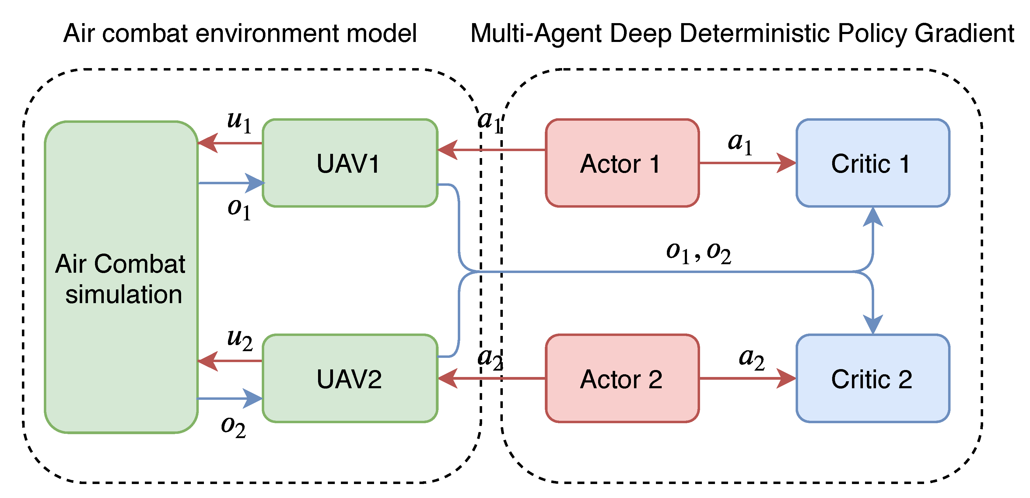
To address the problem of reinforcement learning in a multi-agent environment, Lowe et al. [22] proposed the MADDPG algorithm and applied the DDPG algorithm to a multi-agent environment. The MADDPG algorithm presents the idea of “centralized training, decentralized execution” and learns a centralized Q function for each agent. A MADDPG algorithm that is based on global information can address the non-stationary problems and stabilize training.

Concretely speaking, the study considers the two-player ZSMG as an example of a multi-agent environment and assumes ${\mu }_{a_1}$ to be the agent policy and ${\mu }_{a_2}$ to be the opponent policy. Subsequently, we can write the gradient of the expected return for the agent and opponent with polices ${\mu }_{a_1}$ and ${\mu }_{a_2}$, $J_{a_1}\left({\theta }_{a_1}\right)={\mathbb{E}}_{s\sim {\mathit{\mu }}_{{\mathit{a}}_{\mathbf{1}}},{\mathit{\mu }}_{{\mathit{a}}_{\mathbf{2}}}}\left[G_{a_1}\right]$, $J_{a_2}\left({\theta }_{a_2}\right)={\mathbb{E}}_{s\sim {\mathit{\mu }}_{{\mathit{a}}_{\mathbf{1}}},{\mathit{\mu }}_{{\mathit{a}}_{\mathbf{2}}}}\left[G_{a_2}\right]$ as:

$$\begin{array}{cc}\hfill & {\nabla }_{{\theta }_{a_1}}{J}_{a_1}\left({\theta }_{a_1}\right)={\mathbb{E}}_{s\sim \mathcal{D}}\left[{\nabla }_{\theta }{\mathit{\mu }}_{a_1}\left(s\right){\nabla }_{a_1}{Q}^{{\mathit{\mu }}_{{\mathit{a}}_{\mathbf{1}}}}(s,a_1,a_2){|}_{a={\mathit{\mu }}_{{\mathit{a}}_{\mathbf{1}}}\left(s\right)}\right]\hfill \end{array}$$

(5)

where, $Q^{{\mathit{\mu }}_{{\mathit{a}}_{\mathbf{1}}}}(s,a_1,a_2)$ is a centralized action-value function of an agent that uses the agent and opponent as input and $Q^{{\mathit{\mu }}_{{\mathit{a}}_{\mathbf{2}}}}(s,a_1,a_2)$ is a centralized action-value function of the opponent. The experience replay buffer $\mathcal{D}$ contains the tuples $(s,s^{\prime },a_1,o_2,\mathcal{R})$ recording experiences of the agent and opponent, where $s^{\prime }$ denotes the next state from s after taking actions $(a_1,a_2)$. Centralized action–value functions are updated using the temporal-difference learning. Taking UCAV 1-vs.-1 WVR air combat as an application scenario, both UCAVs will have a Q network and a policy network, respectively. The input of the Q network is the flight status, air combat situation features and action vector of both UCAVs, and the output is Q value of own UCAV. The input of the policy network is the flight status, and the air combat situation features of both UCAVs, and the output is the action vector of own UCAV. A schematic of MADDPG’s idea of “centralized training, distribution execution” of UCAV 1-vs.-1 WVR air combat is illustrated in Figure 1.

3. 1-vs.-1 WVR Air Combat Engagement Modelling

The two players in a 1-vs.-1 WVR aerial combat engagement, referred to as ${\mathrm{UCAV}}_1$ and ${\mathrm{UCAV}}_2$, are assumed to be on the same horizontal plane. The objective of each player is to reach the tail of the adversary and track it in a stable manner, in order to satisfy the shooting condition of the guns.

In the following subsection, the 1-vs.-1 WVR aerial combat is modeled by ZSMG. Moreover, the control decisions of each player are taken in the same discrete time interval.

3.1. Air Combat Reward Function and Termination Condition Designing

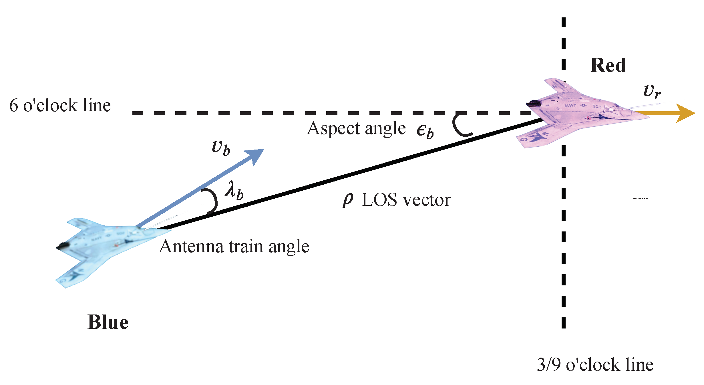
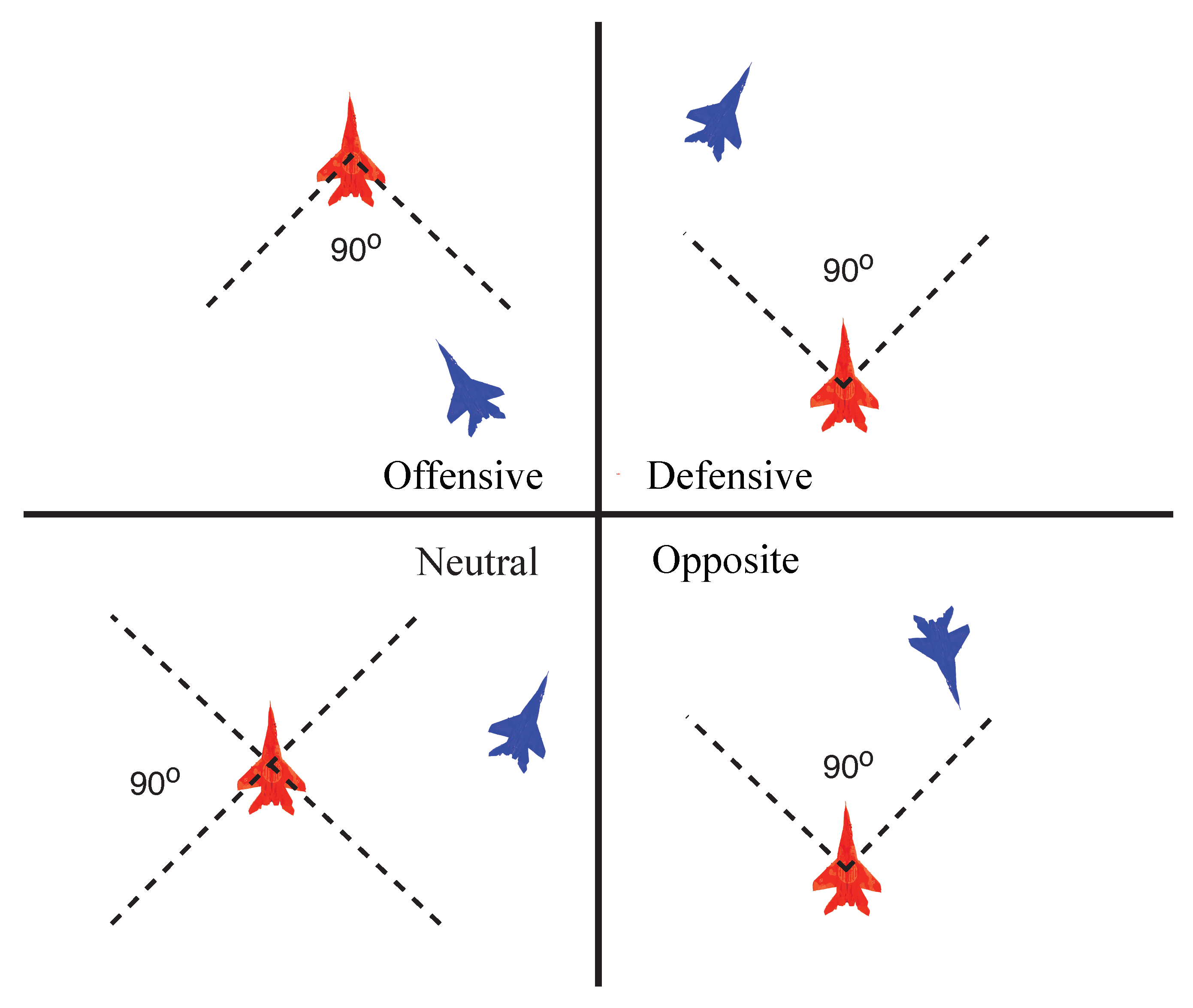
In real 1-vs.-1 WVR air combat scenes, both UCAVs maneuver at the same time and, therefore, one UCAV will be located at the tail of the other UCAV. This ensures stable locking on the other party, then the opponent UCAV is difficult to get rid of the lock and is shot down finally. The combat geometry and parameters shown in Figure 2 are employed.

In Figure 2, ${\lambda }_1$ is the antenna train angle (ATA) of ${\mathrm{UCAV}}_1$, which is the angle between the LOS vector and ${\mathrm{UCAV}}_1$’s velocity vector. ${ϵ}_1$ is the aspect angle (AA) of ${\mathrm{UCAV}}_1$, which is the angle between the LOS vector, and ${\mathrm{UCAV}}_2$’s velocity vector. ${ϵ}_1$ can be obtained in terms of the velocity of vector ${\mathit{V}}_{\mathbf{1}}$ and the line-of-sight (LOS) vector $\mathit{\rho }$, where $\mathit{\rho }$ denotes the LOS vector between ${\mathrm{UCAV}}_1$ and ${\mathrm{UCAV}}_2$. The ATA and AA are allowed to take any value between $\pm {180}^{°}$. ATA and AA can be obtained from Equations (6) and (7).

$${\lambda }_1={cos}^{-1}\left[\frac{{\mathit{V}}_{\mathit{r}}·\mathit{\rho }}{|{\mathit{V}}_{\mathbf{2}}\left|\right|\mathit{\rho }|}\right]$$

(6)

$${ϵ}_1={cos}^{-1}\left[\frac{{\mathit{V}}_{\mathit{b}}·\mathit{\rho }}{|{\mathit{V}}_{\mathbf{1}}\left|\right|\mathit{\rho }|}\right]$$

(7)

As can be seen from Figure 2, a smaller value of $|{\lambda }_1|$ means that ${\mathrm{UCAV}}_1$ or the gun of ${\mathrm{UCAV}}_1$ is more accurate at aiming at ${\mathrm{UCAV}}_2$, so $|{\lambda }_1|$ is inversely proportional to the shooting chance or offensive advantage. Similarly, a smaller $|{ϵ}_1|$ indicates a smaller probability of being hit by ${\mathrm{UCAV}}_2$; therefore, $|{ϵ}_1|$ is inversely proportional to the survival advantage. A termination condition of 1-vs.-1 WVR air combat and rewards can be designed through the abovementioned quantitative analysis of the air combat objectives and related parameters.

This article considers a 1-vs.-1 WVR air combat as a ZSMG problem. Therefore, the rewards of both the UCAVs should be opposite. According to the objective of the 1-vs.-1 WVR air combat, the reward function can be designed using Equation (8), as follows:

$${\mathcal{R}}_1=-{\mathcal{R}}_2=\left\{\begin{array}{cc}1.0,& \left|{\lambda }_1\left(s\right)\right|<{30}^{°}\wedge \left|{ϵ}_1\left(s\right)\right|<{60}^{°}\\ -1.0,& \left|{\lambda }_2\left(s\right)\right|<{30}^{°}\wedge \left|{ϵ}_2\left(s\right)\right|<{60}^{°}\\ 0,& otherwise\end{array}\right.$$

(8)

According to the air combat geometry that is shown in Figure 2, the geometric relationship between AA and ATA of the two UCAVs can be obtained, as follows:

$$\begin{array}{cc}\hfill & |{\lambda }_1\left(s\right)|+|{ϵ}_2\left(s\right)|={180}^{°}\hfill \\ \hfill & |{\lambda }_2\left(s\right)|+|{ϵ}_1\left(s\right)|={180}^{°}\hfill \end{array}$$

(9)

When a UCAV (assumed to be ${\mathrm{UCAV}}_1$) satisfies the condition $\left|{\lambda }_1\left(s\right)\right|<{30}^{°}\wedge \left|{ϵ}_1\left(s\right)\right|<{60}^{°}$ and satisfies this condition for a period of time, it is believed that ${\mathrm{UCAV}}_1$ can maintain the condition and complete the attack and destruction of ${\mathrm{UCAV}}_2$.

3.2. Action Space of 1-vs.-1 WVR Air Combat

In most previous studies [3,4,8], UCAV’s action space was discrete, and basic fighter maneuvering (BFM) was used as an air combat maneuvering action space, which includes nine actions: left climb, climb, right climb, horizontal left turn, horizontal forward flight, horizontal right turn, dive left, dive, dive right. Although these nine actions cover all common maneuvering actions of a UCAV, the parameters for these maneuvering actions are fixed, and the maneuvering parameters cannot be changed quantitatively, and cannot be combined.

In this paper, a continuous action space is used to control the UCAVs. As air combat is carried out in the same horizontal plane, there are two continuous control variables which control UCAV, namely the thrust and the roll rate. The pitch angular velocity and yaw angular velocity are not considered. Therefore, the action space can be indicated by:

$$(u_t,u_{\dot{\psi }})$$

(10)

where, $u_t$ is the thrust of a UCAV and $u_{\dot{\psi }}$ is the roll rate of a UCAV. They have upper and lower limits, and their upper and lower limits will vary depending on the performance of the UCAV. Together, they will affect the performance of a UCAV’s acceleration and turning maneuvers.

3.3. State Space of 1-vs.-1 WVR Air Combat

System state of air combat is defined by the current motion state parameters of ${\mathrm{UCAV}}_1$ and ${\mathrm{UCAV}}_2$, the relative position and angle parameters and future motion state parameters. Firstly, the current motion state parameters of the two UCAVs in air combat are considered to form the basic state space ${\mathcal{S}}_{base}$:

$${\mathcal{S}}_{base}={\left[x_1,y_1,x_2,y_2,v_1,v_2,{\varphi }_1,{\varphi }_2,{\psi }_1,{\psi }_2\right]}^T$$

(11)

where, $(x_1,y_1)$ and $(x_2,y_2)$ are the current positions of ${\mathrm{UCAV}}_1$ and ${\mathrm{UCAV}}_2$. The positions of UCAVs have no limits, thereby allowing for flight in all directions in the x-y plane. Notably, $v_1$ and $v_2$ are the current speeds of both UCAVs, ${\varphi }_1$ and ${\varphi }_2$ are the current heading angles of both UCAVs, and ${\psi }_1$ and ${\psi }_2$ are the current bank angles of both UCAVs. The bank angle is limited based on the maximum capabilities of the actual UCAV, and based on the need to limit the maximum turning capabilities of the UCAV, the heading angle is allowed to take any value between $\pm {180}^{°}$.

Subsequently, the distance and relative angle parameters of the two UCAVs are introduced as components of the state space of 1-vs.-1 WVR air combat. The distance parameter is the two-norm of the LOS vector $\mathit{\rho }$, and the relative angle parameters are $\lambda$ and $ϵ$. These components of the state space are depicted in Equation (12):

$${\mathcal{S}}_{relative}={\left[\left|\mathit{\rho }\right|,{\lambda }_1,{\lambda }_2,{ϵ}_1,{ϵ}_2\right]}^T$$

(12)

Finally, a prediction of the target position is introduced, and the predicted target position is used as a component of the state space. A precise prediction of the target’s future position is crucial for preemptive action. However, accurate predictions can be difficult to achieve owing to uncertainty of the target’s position and intention. The exact model and the characteristics of a combat aircraft are completely hidden. Due to individual differences in the behaviors of the pilots, the combat strategies can contain unpredictable randomness. Furthermore, wrong predictions can worsen the combat situation. Therefore, the target positions should be carefully and precisely predicted.

3.3.1. Prediction Interval Estimation

The size of the prediction interval directly affects the accuracy and computational complexity of the target predictions. If the selected time interval is extremely large, there will be a large difference between the actual position of the target in the future and predicted position; this will impact the obtained air combat countermeasures. If the selected time interval is extremely small, the predicted position will be too close to the current position and, in this case, target prediction cannot be applied. In this study, the flight time required for a bullet to hit the enemy is set to the prediction interval $T_p$.

$$T_p=\frac{\left|\mathit{\rho }\right|}{V_{bullet}}$$

(13)

3.3.2. Target Position Prediction

Before predicting the location of a target, it is necessary to assume that the target maneuvering is rational, and that the future control signal of the target only adds a small perturbation $\widehat{\mathit{ϵ}}$ based on the current control signal. The specific calculation of the perturbation $\widehat{\mathit{ϵ}}$ will be explained in Section 3.3. After calculating the perturbation, the predicted target position can be calculated while using Algorithm 1. Because the value of the perturbation is not strong and the prediction interval is small, the explicit single-step method (Euler’s method) should be used to solve the UCAV motion differential equations.

In Algorithm 1, $T_p$ is the prediction interval, $x,y,v,\varphi ,\psi$ are the current motion states of the target UCAV, and $\delta t$ is the step time of solving differential equations, $x_p,y_p$ is the predicted position of the target UCAV. The components of the state space are included in Equation (14):

$${\mathcal{S}}_{predict}={\left[T_p,x_p,y_p\right]}^T$$

(14)

In summary, the three state space components of the current motion states, relative to the position and angle states and future motion states, are combined in order to obtain the overall state space:

$$\mathcal{S}={\mathcal{S}}_{base}\oplus {\mathcal{S}}_{relative}\oplus {\mathcal{S}}_{predict}$$

(15)

where, ⊕ is the operator for linking two column vectors.

Algorithm 1: Target position prediction

4. Maneuvering Policy Generation Algorithm Designing in 1-vs.-1 WVR Air Combat Based on MADDPG

4.1. Maneuvering Strategy Generation Algorithm Outline

The algorithm framework is composed of the air combat environment model, MADDPG, reward shaping, and target position predication modules. Specifically, we introduced the future position of the target UCAV in the MADDPG algorithm. It should be noted that, unlike the traditional MADDPG algorithm, when using the air combat strategy generated by this algorithm, the Q-network after training is still required in order to predict the target’s future position. Moreover, we Introduce potential-based reward shaping method to improve the efficiency of maneuver strategy generation algorithm of UCAV. Figure 3 shows the overall framework of the maneuvering strategy generation algorithm.

In Figure 3, the upper left part denotes the air combat environment model, and its input are the actions of both the UCAVs, and the output are the next motion states s and the reward values of the UCAVs. The upper right part denotes the MADDPG algorithm module, which contains two actors and two critics.

The actor’s input is the state vector $\mathcal{S}$ described in Section 3.3, and the output is the action vector $\mathit{a}$ described in Section 3.2. Two neural networks are used in the actor, one as the target network and the other as the online network, in order to improve the stability of the learning process. The structures of the two networks are the same, but the update methods are different. The online network uses the deterministic policy gradient for updating, and the target network copies the parameters of the online network through soft updates.

The critic’s inputs are the state vector $\mathcal{S}$ and two action vectors $a_1,a_2$, and the output is the $Q(s,a_1,a_2)$ value. Similar to the actor, there are two neural networks in the critic, one for the target network and the other for the online network. The update method is also similar to that used in the case of the actor. However, the difference lies in that the input during updating is sampled from the prioritized replay memory.

The inputs of the reward shaping module are the state vector $\mathcal{S}$ and the reward value r. The shaping reward is a designed reward that is received from the air combat environment. The specific method of designing the shaping reward is explained in Section 4.2. The input to the target prediction module are the state vector ${\mathcal{S}}_{base}$, $-\alpha {\nabla }_{a_1}{Q}^{{\mathit{\mu }}_{{\mathit{a}}_{\mathbf{2}}}}(s,a_1,a_2)$ and $-\alpha {\nabla }_{a_2}{Q}^{{\mathit{\mu }}_{{\mathit{a}}_{\mathbf{1}}}}(s,a_1,a_2)$, and the output is the vector of predicted target position ${\mathcal{S}}_{predict}$. The method for target position prediction is explained in Section 4.3. Algorithm 2 explains the MADDPG training process for 1-vs.-1 WVR air combat engagement.

Algorithm 2: Multi-agent deep deterministic policy gradient (MADDPG) Training process for 1-vs.-1 within visual range (WVR) air combat engagement

4.2. Reward Shaping

Deep reinforcement learning (DRL) has always suffered from restricted practical applications owing to its high requirements in terms of training time and computational power. For example, the training of AlphaZero training required a considerable amount of computational power, and the training period was three days. Therefore, shortening of the training time is a prominent issue in this field.

Directly training an air combat maneuvering strategy in 1-vs.-1 WVR air combat is challenging because its reward function is very sparse. Therefore, in this study, a reward shaping method is proposed in order to accelerate the training process and, consequently, shorten the training time.

Shaping reward is a reward for designers’ rewards for nature’s gains from the environment. Shaping reward provide a visual representation of the domain knowledge, especially for designers who may have already designed the environmental rewards [23]. In addition, it does not require the modification of the agent or environment, thereby resulting in a relatively simple implementation. However, if the design of the shaping reward is inappropriate, then it may slow down the convergence time of the training algorithm or even lead to failure of the policy to converge to Nash equilibrium.

Potential-based reward shaping (PBRS) is proposed for the above problem [24]. The shaping reward ${\mathcal{R}}_{rs}$ given in this approach is the difference of a potential function $\mathsf{\Phi }$ defined over a source state s and a destination state $s^{\prime }$:

$${\mathcal{R}}_{rs}=\mathcal{R}+\gamma \mathsf{\Phi }\left(s\right)-\mathsf{\Phi }\left(s^{\prime }\right)$$

(17)

where $\mathcal{R}$ is the original reward from the environment and $\gamma$ is the discount factor in the MADDPG algorithm.

PBRS has been proven to not change the Nash equilibrium of multi-agent systems; however, it affects the exploration of shaping agents [25]. Therefore, it can change the convergence of the joint policy, because a modification in the exploration of one agent can entirely redirect the search of the joint policy space to different equilibrium points. Therefore, we need to combine prior knowledge of air combat in order to design a shaped reward that allows two UCAVs to converge to a better Nash equilibrium policy.

4.2.1. Reward Shaping for Orientation

In an actual air combat scenario, the purpose of two UCAVs is to enter the opponent’s tail attack zone and stabilize the position of the opponent, so that the UCAVs can launch short-range combat air-to-air missiles and effectively attack the enemy UCAV. For this purpose, the ATA $\lambda$ and AA $ϵ$ of the UCAV are made as small as possible. The reward shaping of orientation for ${\mathrm{UCAV}}_1$ can be designed, as follows:

$${\mathsf{\Phi }}_o\left(s\right)=\frac{{180}^{°}-\left(\right|{\lambda }_1\left(s\right)|+|{ϵ}_1\left(s\right)\left|\right)}{{180}^{°}}$$

(18)

The range of ${\mathsf{\Phi }}_o\left(s\right)$ is $[-1,1]$. ${\lambda }_1\left(s\right)$ and ${ϵ}_1\left(s\right)$ can be calculated from the current system state s while using the following formula:

$$\begin{array}{cc}\hfill & |{\lambda }_1\left(s\right)|=|{\varphi }_1-{\tau }_1\left(s\right)|\hfill \\ \hfill & |{ϵ}_1\left(s\right)|=|{\varphi }_2-{\tau }_1\left(s\right)|\hfill \\ \hfill & {\tau }_1\left(s\right)={tan}^{-1}\left(\frac{y_2-y_1}{x_2-x_1}\right)\hfill \end{array}$$

(19)

4.2.2. Reward Shaping for Distance

In air combat, both the missile and cannon of the UCAV have corresponding attack distances, including the maximum and the minimum attack distances, the inescapable distance, and so on. Hence, reward shaping for distance needs to be designed such that the UCAV tends to complete the desired distance $D_e$. Reward shaping for distance can be designed using the following equation:

$$\begin{array}{cc}\hfill & {\mathsf{\Phi }}_d\left(s\right)={\mathsf{\Phi }}_o\left(s\right){exp}^{-k_d|D_e-D\left(s\right)|}\hfill \end{array}$$

(20)

where, $D\left(s\right)=\sqrt{{(x_1-x_2)}^2+{(y_1-y_2)}^2}$ is the distance between the two UCAVs and $k_d$ is a coefficient. Furthermore, the range of ${\mathsf{\Phi }}_d\left(s\right)$ is $[-1,1]$. The reward shaping for distance can effectively adjust the distance of the two UCAVs according to the current air combat situation. For example, if ${\mathrm{UCAV}}_1$ is in the defensive position, then the distance much be increased as much as possible to move away from ${\mathrm{UCAV}}_2$; if ${\mathrm{UCAV}}_1$ is in the offensive position, the distance needs to be decreased as much as possible to be at the desired position.

4.2.3. Reward Shaping for Velocity

The current air combat situation determines the expected velocity of a UCAV. For example, when ${\mathrm{UCAV}}_1$ is in the offensive situation, the expected velocity of ${\mathrm{UCAV}}_1$ needs to be the same as that of ${\mathrm{UCAV}}_2$, in order to prevent overshooting caused by a very high velocity, and to prevent being thrown off by ${\mathrm{UCAV}}_2$ caused by a very low velocity. On the contrary, when ${\mathrm{UCAV}}_1$ is in the defensive situation, the velocity of ${\mathrm{UCAV}}_1$ needs to be different from that of ${\mathrm{UCAV}}_2$, such that it is possible to change from a defensive position to an offensive one through a change in velocity. Reward shaping for velocity can be designed while using the following equation:

$$\begin{array}{cc}\hfill & {\mathsf{\Phi }}_v\left(s\right)={\mathsf{\Phi }}_o\left(s\right){exp}^{-k_v|v_1-v_2|}\hfill \end{array}$$

(21)

where, $k_v$ is a coefficient, and the range of ${\mathsf{\Phi }}_v\left(s\right)$ is $[-1,1]$.

4.2.4. Combined Reward Shaping

The reward shaping components, Equations (18), (20) and (21), can be combined to obtain the resultant reward shaping:

$$\mathsf{\Phi }\left(s\right)={\mathsf{\Phi }}_o\left(s\right)+{\mathsf{\Phi }}_d\left(s\right)+{\mathsf{\Phi }}_v\left(s\right)$$

(22)

4.3. Target Position Prediction

The air combat strategy needs to quickly occupy a dominant position and attack the target if required in order to enable the learned air combat strategy of a UCAV to acquire the intent of the target UCAV and perform predictive maneuvers. In this section, we will discuss the method of target position prediction. As we already explored the algorithm framework for predicting the target position in Section 3.2, in this section, we will mainly focus on the calculation of perturbation.

We assume that the air combat strategy of UCAVs on both sides of the battlefield is completely rational. Subsequently, the maneuvering action of one UCAV will minimize the Q function value of the other UCAV. For clarity, we assume ${\mathrm{UCAV}}_1$ to be our UCAV and ${\mathrm{UCAV}}_2$ to be the target UCAV. When ${\mathrm{UCAV}}_1$ takes action $a_1$, then ${\mathrm{UCAV}}_2$’s action in the next moment, $a_2^{*}$, can be described by Equation (23).

$$a_2^{*}=\underset{a_2}{argmin}{Q}^{{\mu }_1}(s,a_1,a_2)$$

(23)

Likewise, from the viewpoint of ${\mathrm{UCAV}}_2$, Equation (24) can be used to predict the action of ${\mathrm{UCAV}}_1$.

$$a_1^{*}=\underset{a_1}{argmin}{Q}^{{\mu }_2}(s,a_1,a_2)$$

(24)

The critical challenge in our proposed method of action prediction of the opponent UCAV is the minimization expressed in Equations (23) and (24). The direct optimization of minimization is difficult owing to the non-linearity of the continuous action space and the Q function. A simple approximate solution can be found using an inner-loop gradient descent while performing an update step in Equation (23) or Equation (24); however, this is too computationally expensive for practical use. To simplify the calculation, a simple linear local optimal solution is herein presented. The main concept behind the solution can be summarized in two steps: (1) approximate the non-linear Q function using a locally linear function; (2) replace the inner-loop minimization with a 1-step gradient descent. Note that the core idea is the locally linearized Q function adapted from recent adversarial training techniques originally developed for supervised learning. We use this function to derive an approximation $\widehat{\mathit{ϵ}}$ for the worst-case perturbation by taking

$${\widehat{ϵ}}_{a_2}=-\alpha {\nabla }_{a_2}{Q}^{{\mu }_{a_1}}(s,a_1,a_2)$$

(25)

$${\widehat{ϵ}}_{a_1}=-\alpha {\nabla }_{a_1}{Q}^{{\mu }_{a_2}}(s,a_1,a_2)$$

(26)

where $\alpha$ is the adjustable coefficient representing the perturbation rate. This can also be explained as the step size of the gradient descent. When $\alpha$ is small, the local approximation error is also small, but, because the perturbation is extremely small, it can be assumed that the target is merely following the current maneuver. When $\alpha$ is large, the approximation error may disturb the entire learning process, and the agent may not be able to learn a good policy.

4.4. Prioritized Replay Memory

Prioritized experience replay memory (PERM) is a method of sampling based on experience replay and was proposed by Google DeepMind (London, UK) [26]. Experience replay enables online reinforcement learning agents to remember and reuse experiences from the past. In previous studies, experience transitions were uniformly sampled from a replay memory. However, this approach simply replays the transitions in the same frequency that they were originally experienced in, regardless of their significance. PERM can sample experiences, more frequently prioritize to replay critical transitions, and therefore learn more efficiently.

5. Simulation and Analysis

5.1. Platform Setting

5.1.1. Air Combat Simulation Platform Construction

The air combat simulation platform was built using the Python programming language and the HARFANG three-dimensional (3D) framework, which is a software framework that is used for the development of modern multimedia applications and for modeling the shapes of aircrafts. The HARFANG framework can manage and display complex 3D scenes, play sounds and music, and access virtual reality (VR) devices, such as the Oculus Rift. It is a new multimedia application development framework, which is highly suitable for the development of games; it also provides appropriate support for VR equipment. Nowadays, ground controllers use VR equipment to control the UCAVs; hence, we adopted the HARFANG 3D framework for our proposed air combat simulation platform.

The platform was able to simulate the 1-vs.-1 WVR air combat in certain airspaces, use the dynamic equation with three degrees of freedom to simulate the flight characteristics of UCAV, and set the performance parameters of both the UCAVs. The platform was also able to reserve the air combat strategy interface of the two UCAVs, thereby obtaining the UCAV control signals from the external environment. The platform could also support human control, where the interface received input from a keyboard or hands-on throttle and stick system (HOTS).

Figure 4 depicts the main interface of the air combat simulation platform. The interface presents a real-time combat situation of the UCAVs, and the five positions on the screen display the health value, altitude and speed, radar image, attitude angle, and all of the speed components.

5.1.2. Maneuvering Strategy Generation Algorithm Parameters Setting

According to the definition of a state space and an action space, it is obvious that the length of the actor network’s input vector is 18, and that of the output vector is 2. The length of the critic network’s input vector is 22, and that of the output vector is 1.

The online actor network, target actor network, online critic network, and target critic network are constructed using a fully connected neural network. Figure 5 depicts the structures of the actor and critic networks. The output layer of the actor network and the critic network have no activation function; furthermore, the remaining layers are all ReLU layers. The learning rate of the network is $0.01$, and the discount factor is $\gamma =0.9$. The soft update factor of the target network is $0.01$. Additionally, the weight of the initialized neural network can be adjusted to be using the Xavier initializer. The batch size of the updating network is 1024, and the size of the prioritized experience replay memory is set to ${10}^6$. The coefficient of the perturbation rate $\alpha$ is 0.5.

In a 1-vs.-1 WVR air combat simulation process, the decision period is set to 1 s and the number of maximum step of an episode is set to 150. In an episode simulation, if a UCAV satisfies Equation (8) for five consecutive steps, the episode is terminated, and the UCAV wins the air combat. If there is no win or loss beyond the maximum stride length, then the air combat is considered to be a tie.

5.1.3. Initial Setting for 1-vs.-1 WVR Air Combat Engagement

As in [27], Figure 6 shows the four different initial conditions of the 1-vs.-1 WVR air combat engagement based on the initial relative positions and orientations of the UCAVs. The initial position of ${\mathrm{UCAV}}_1$ with respect to ${\mathrm{UCAV}}_2$ in the horizontal direction is randomly chosen to be between 350 and 1050 m in the offensive, defensive, and neutral cases. The two UCAVs are at the same height, as this study only considers maneuver strategies in the horizontal plane.

5.1.4. UCAV Performance Parameters Setting

For experimental comparison, two different UCAV performance parameters were considered in this study. The variation of the performance capabilities focus on the following parameters: maximum thrust and maximum roll rate, as presented in

Table 1. Unmanned combat air vehicles (UCAV) performance parameters setting.

Parameter	Advantage Value	Disadvantage Value
Maximum roll rate (deg/s)	140	110
Maximum thrust (N)	100,000	80,000

. The dominant UCAV performance parameters are called the “advantage” parameters, and the non-dominant UCAV performance parameters are called the “disadvantage” parameters. The mass of both the UCAVs is same and equal to 10,000 kg.

5.1.5. Evaluation Metrics of Air Combat Strategy

The most direct method for evaluating an air combat strategy is to conduct an air combat confrontation with other air combat strategies and then determine the winner. We can also determine whether the flight track generated by an air combat strategy is reasonable by observing the flight tracks of the UCAVs from both sides of the combat.

To quantitatively and accurately analyze the intelligence degree of an air combat strategy, this study proposes the use of four metrics: intercept time $T_I$, defensive time $T_D$, offensive time $T_O$, and winning probability $P_W$. The intercept time is measured from the beginning of the air combat simulation until a UCAV has established a position of advantage. The position of advantage is the termination condition of the air combat, expressed in Equation (8). Defensive time is the time when a UCAV is at $\left|AA\right|>{90}^{°}$ during an air combat. Offensive time is the time when a UCAV is at $\left|ATA\right|<{90}^{°}$ during an air combat. The winning probability is the ratio of the number of air combat simulations and the total number of air combat simulations.

5.2. Maneuvering Strategy Training and Testing

5.2.1. Comparative Analysis of Training Process

In this section, a comparative analysis of the training methods is performed. These three training algorithms are the basic MADDPG algorithm (MADDPG), the MADDPG algorithm with only reward shaping (RS-MADDPG), and the MADDPG algorithm with reward shaping and prediction of the target position (PRED-RS-MADDPG).

When training the air combat countermeasures, the initial states of the two UCAVs are randomly generated according to the four situations described in Section 5.1.3. At the same time, to prevent the two UCAVs from falling into the “boring” Nash equilibrium of “biting the tail” during training, the performance parameters of the two UCAVs to be different from one another: one UCAV uses the “advantage” performance parameters, and the other UCAV uses the “disadvantage” performance parameters.

Figure 7 depicts the curve of the normalized average reward of MADDPG, RS-MADDPG, and PRED- RS-MADDPG about the episodes, which is one complete play of the UCAVs interacting with the air combat environment. The reason for normalization is that, after reward shaping, there is no guarantee that the reward per step is between $[-1,1]$. As the problem is a two-player ZSMG, the average reward of the two UCAVs will be negative to each other. Therefore, in Figure 7, only the average reward of the UCAV with an advantageous performance is plotted.

The naive MADDPG algorithm does not work, and its average reward value is always kept around 0, which is unreasonable, as can be seen from Figure 7. The reason why the algorithm is invalid is that the algorithm uses a sparse reward function. When the reward is sparse, the effective policy learning information is little, which makes the algorithm invalid. As the performance parameters of the UCAVs of both the sides are different, the average reward value gradually converges to a positive value. By comparing the RS-MADDPG algorithm with the PRED-RS-MADDPG algorithm, it can be determined that the training convergence speed of the PRED-RS-MADDPG algorithm is slightly better than that of the RS-MADDPG algorithm. A possible reason is that the Q value error on both sides of the Q network output in the early stage of training is large; the Q value gradient error is also large, which affects the accuracy of the predicted target position and, hence, slows the training speed of the RS-MADDPG algorithm. However, the average reward of the PRED-RS-MADDPG algorithm is higher than that of the RS-MADDPG algorithm. This shows that, by predicting the target position, the UCAV on the advantage side can quickly lock the target and complete the attack necessary to win the air battle. Regarding the essential reason for converging to a better average reward, we believe that the introduction of the target’s position prediction provides more target information for our UCAV, which will enable the air combat strategy to achieve a better equilibrium strategy.

5.2.2. PRED-RS-MADDPG Strategy vs. Simple Script Strategies

In this section, the intelligence degree of the 1-vs.-1 WVR air combat strategy obtained while using the PRED-RS-MADDPG algorithm is evaluated with respect to a few simple script strategies. Three basic scripting strategies were proposed: the “uniform linear motion” strategy, the “decelerate left turn” strategy, and the “S-type maneuver” strategy. The performance parameters of UCAVs on both sides are kept at “advantage” to ensure that the performance of the two UCAVs is the same. Meanwhile, the initial position of each UCAV is set to face each other; the initial speed is the same, which results in an absolutely equal initial state. The “uniform linear motion” strategy is to keep the speed of UCAV at 180 km/h. The “decelerate left turn” strategy is to keep the UCAV accelerating to the left. The “S-type maneuver” strategy means the UCAV turns from left to right every 15 s and then from the right to left every 15 s. “Decelerate left turn” strategy and “S-type maneuver” are often used in real air combats.

Figure 8, Figure 9 and Figure 10 show the fly trajectory and the change in air combat situation of the 1-vs.-1 WVR air combat strategy obtained by using the PRED-RS-MADDPG algorithm against the “uniform linear motion” strategy, “decelerate left turn” strategy, and “S-type maneuver” strategy. In general, a UCAV using the PRED-RS-MADDPG strategy can achieve termination and win the air combat against UCAVS having any of the three basic scripting strategies. In Figure 9, at 5 s, ${\mathrm{UCAV}}_1$ realizes that ${\mathrm{UCAV}}_2$ will turn left, and then immediately turns right and, at 20 s, it turned left to enter the turning circle of ${\mathrm{UCAV}}_2$, then stable tracking was conducted after 35 s. This indicates that ${\mathrm{UCAV}}_1$ had a reasonable prediction of ${\mathrm{UCAV}}_2$’s maneuvers at 5 s, which is very similar to the maneuvering of manned aircrafts in 1-vs.-1 WVR air combat. In Figure 10, an interesting situation was observed. At 10 s, ${\mathrm{UCAV}}_1$ did not turn right with ${\mathrm{UCAV}}_2$, but turned left. This situation is not easy to understand from a bystander’s perspective. It is assumed that at 10 s, ${\mathrm{UCAV}}_1$ predicts that ${\mathrm{UCAV}}_2$ will turn left in the future to cause ${\mathrm{UCAV}}_1$ overshoot. Hence, ${\mathrm{UCAV}}_1$ also turned left to respond. This situation occurs when the target UCAV is not completely rational, which will cause the error in predicting the target position to be very large, which results in erroneous maneuvering. However, overall, ${\mathrm{UCAV}}_1$ corrected its erroneous maneuver in time and, finally, won the air combat.

Table 2. Evaluation metrics of the air combat strategy.

Evaluation Metrics	Uniform Linear Motion	Decelerate Left Turn	S-Type Maneuver
Intercept time $T_I$	40 s	45 s	50 s
Defensive time $T_D$	0 s	1 s	0 s
Offensive time $T_O$	26 s	32 s	26 s

shows the evaluation metrics of the air combat strategy.

In Table 2, the offensive time accounts for more than 50% of the total intercept time, which indicates that the UCAV has a very efficient attack capability against the basic scripted air combat strategy.

5.2.3. PRED-RS-MADDPG Strategy vs. RS-MADDPG Strategy

It can be proved that the PRED-RS-MADDPG strategy can outperform the script strategies with a great advantage, thereby indicating that the strategy obtained using the PRED-RS-MADDPG algorithm is highly effective. In this section, to test whether the intelligence of the strategy has improved after the introduction of target prediction, air combat confrontation experiments using the PRED-RS-MADDPG strategy vs. the RS-MADDPG strategy were designed and performed. To ensure that objectivity is maintained, the performance parameters of both the UCAVs were kept the same; both used the “advantage” parameters. Subsequently, two fair air combat situations were selected as the initial air combat situations: opposite situation and neutral situation. Figure 11 and Figure 12 show the fly trajectory and the change in air combat situation of the 1-vs.-1 WVR air combat strategy obtained using the PRED-RS-MADDPG algorithm against the RS-MADDPG strategy in the opposite and the neutral initial situation, respectively. In Figure 11 and Figure 12, the blue line is the fly trajectory of the UCAV using PRED-RS-MADDPG strategy, and the red line is the fly trajectory of the UCAV using RS-MADDPG strategy.

In Figure 11, ${\mathrm{UCAV}}_1$ took a left-turn action to perform a tactical evasion at the beginning of the air combat; ${\mathrm{UCAV}}_2$ adopted a strategy of confronting the enemy at the beginning of the air combat. After 20 s, ${\mathrm{UCAV}}_1$ was in a defensive situation. ${\mathrm{UCAV}}_1$ kept turning left between 0 to 40 s. When ${\mathrm{UCAV}}_2$ was beyond the 3 o’clock line of ${\mathrm{UCAV}}_1$, ${\mathrm{UCAV}}_1$ immediately turned right until it locked onto the target. During this period, ${\mathrm{UCAV}}_2$ changed from attack to defense mode after 20 s.

In Figure 12, ${\mathrm{UCAV}}_1$ and ${\mathrm{UCAV}}_2$, respectively, turn left and right to attack each other. At 20 s, if ${\mathrm{UCAV}}_1$ continues to turn left, then ${\mathrm{UCAV}}_2$ can track ${\mathrm{UCAV}}_1$ steadily by accelerating the left turn, so that ${\mathrm{UCAV}}_2$ will win. However, in 20 s, ${\mathrm{UCAV}}_1$ predicted that ${\mathrm{UCAV}}_2$ would turn left to put itself in a defensive situation, so it performed a large maneuver to turn right, forcing ${\mathrm{UCAV}}_2$ to also turn right. Afterwards, at 40 s ${\mathrm{UCAV}}_1$ entered ${\mathrm{UCAV}}_2$’s turning circle and successfully locked onto ${\mathrm{UCAV}}_2$.

Through the aforementioned analysis, we concluded that, even if ${\mathrm{UCAV}}_1$ and ${\mathrm{UCAV}}_2$ are in an absolutely equal air combat situation, ${\mathrm{UCAV}}_1$ can still win, which shows that the introduction of the target position prediction can, in fact, effectively improve the intelligence of air combat strategies.

An initial air combat situation was randomly generated and multiple simulations were used to determine the intercept time $T_I$, defensive time, offensive time $T_O$, and the probability of winning $P_W$ in order to quantitatively analyze the degree of improvement. Consequently, initial opposite situations, initial offensive situations, initial defensive situations, and initial neutral situations, were obtained, each a 100 times. The intercept time obtained in the simulation of the winning air combat was noted, because, if the air combat fails, then the intercept time is infinite. A comparison of the intercept time $T_I$, defensive time, and offensive time $T_O$ of the air combat simulations between the PRED-RS-MADDPG strategy and the RS-MADDPG strategy is depicted in Figure 13, and the probabilities of winning $P_W$ as per the results of the air combat simulations are presented in

Table 3. Probability of winning $P_W$ of the air combat simulations.

	Opposite	Offensive	Defensive	Neutral
$P_W$	79%	99%	63%	75%

.

Regardless of the initial air combat situations, PRED-RS-MADDPG strategy wins air combats with a high probability, thereby indicating that an air combat strategy with target maneuver prediction is significantly better than the one that does not utilize target maneuver prediction, as can be seen from Figure 13 and Table 3. When the strategy is integrated with the target maneuver prediction method, the total probability of winning reaches 78.5%.

6. Conclusions

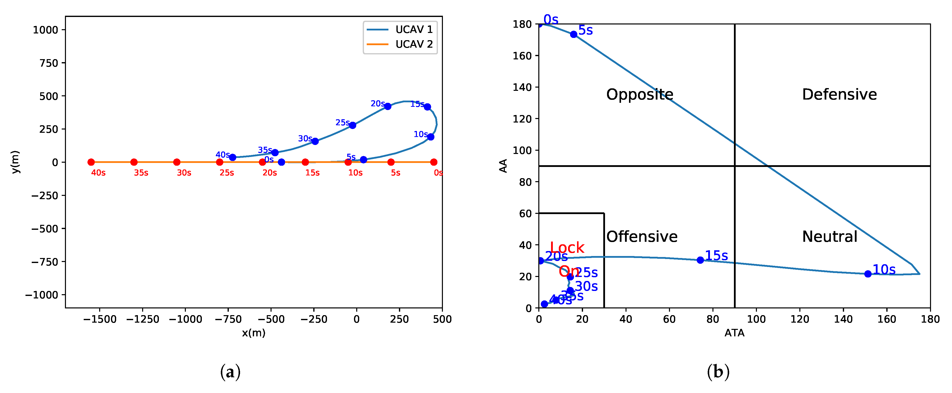
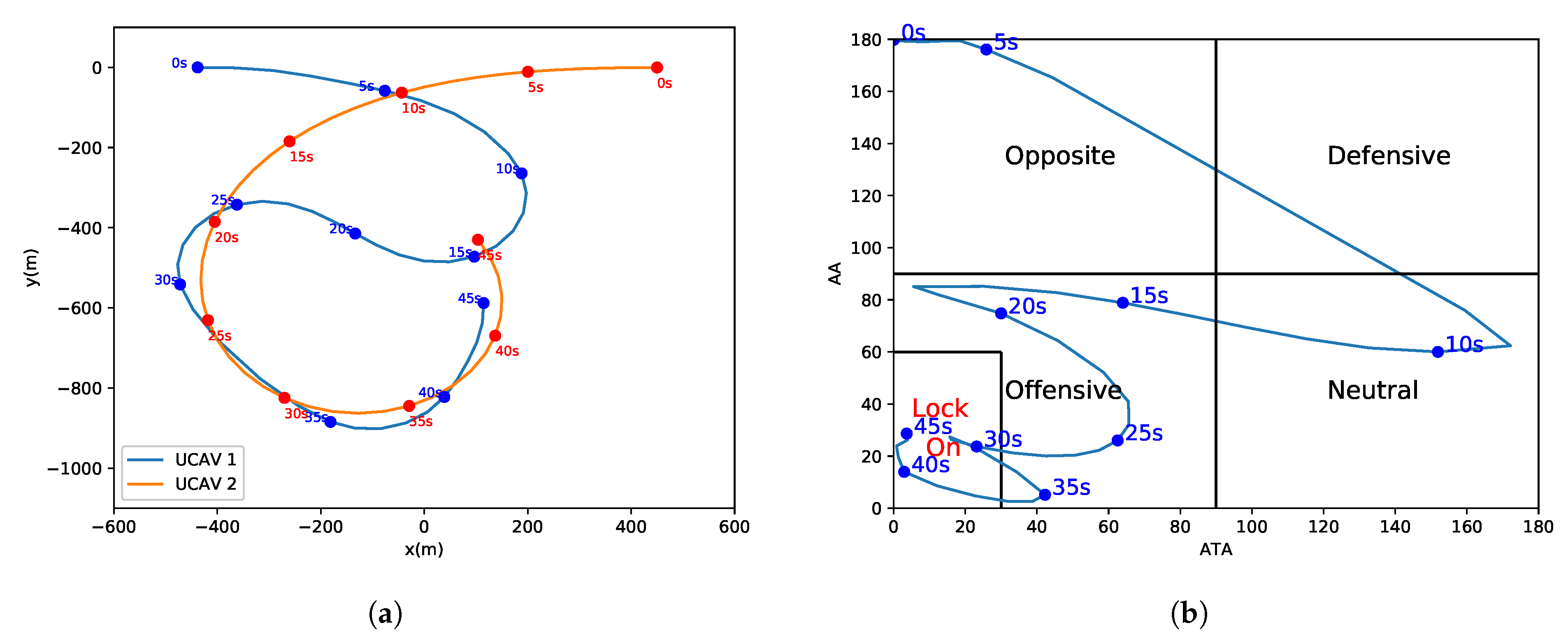
In this study, a design for a maneuvering strategy generation algorithm for 1-vs.-1 WVR air combat is proposed that is based on the MADDPG algorithm. A 1-vs.-1 WVR air combat is modeled as a two-player zero-sum Markov game. To enable the UCAV to predict the maneuver of the target, a method for predicting the future position of the target is introduced. Inspired by adversarial learning, local minimization is used for solving the Q network to predict the future position of the target. At the same time, a potential-based reward shaping method is designed to improve the efficiency of the maneuvering strategy generation algorithm.

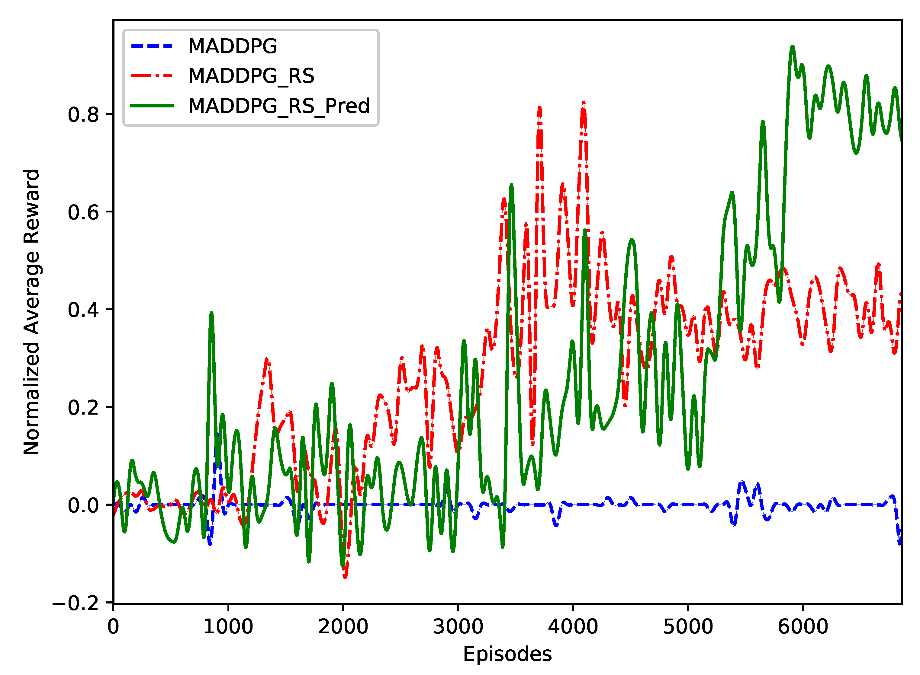
We designed several simulation experiments to verify the effectiveness of the algorithm, as well as the intelligence level of the obtained air combat strategy. The results showed that the strategy obtained while using the PRED-RS-MADDPG algorithm is better than the ones obtained using MADDPG and RS-MADDPG.

In the future, we will focus on applying this method to multi-UCAVs air combat confrontation scenarios. We also intend to use both offline learning and online learning methods in order to obtain a more robust air combat strategy.

References

1. Guo, H.; Zhou, D.; Zhang, K. Study on UCAV autonomous air combat maneuvering decision-making. Dianguang yu Kongzhi (Electron. Opt. Control) 2010, 17, 28–32. [Google Scholar]
2. Duan, H.; Wei, X.; Dong, Z. Multiple UCAVs cooperative air combat simulation platform based on PSO, ACO, and game theory. IEEE Aerosp. Electron. Syst. Mag. 2013, 28, 12–19. [Google Scholar] [CrossRef]
3. Yang, Q.; Zhang, J.; Shi, G.; Hu, J.; Wu, Y. Maneuver Decision of UAV in Short-Range Air Combat Based on Deep Reinforcement Learning. IEEE Access 2019, 8, 363–378. [Google Scholar] [CrossRef]
4. Austin, F.; Carbone, G.; Falco, M.; Hinz, H.; Lewis, M. Automated maneuvering decisions for air-to-air combat. In Proceedings of the Guidance, Navigation and Control Conference, Monterey, CA, USA, 17–19 August 1987; p. 2393. [Google Scholar]
5. Burgin, G.H.; Sidor, L. Rule-Based Air Combat Simulation; Technical Report; Titan Systems Inc: La Jolla, CA, USA, 1988. [Google Scholar]
6. Kelly, M.J. Performance measurement during simulated air-to-air combat. Hum. Factors 1988, 30, 495–506. [Google Scholar] [CrossRef]
7. Shin, H.; Lee, J.; Kim, H.; Shim, D.H. An autonomous aerial combat framework for two-on-two engagements based on basic fighter maneuvers. Aerosp. Sci. Technol. 2018, 72, 305–315. [Google Scholar] [CrossRef]
8. McGrew, J.S.; How, J.P.; Williams, B.; Roy, N. Air-combat strategy using approximate dynamic programming. J. Guidance Control Dynam. 2010, 33, 1641–1654. [Google Scholar] [CrossRef] [Green Version]
9. Yang, Z.; Zhou, D.; Piao, H.; Zhang, K.; Kong, W.; Pan, Q. Evasive Maneuver Strategy for UCAV in Beyond-Visual-Range Air Combat Based on Hierarchical Multi-Objective Evolutionary Algorithm. IEEE Access 2020, 8, 46605–46623. [Google Scholar] [CrossRef]
10. Poropudas, J.; Virtanen, K. Game-theoretic validation and analysis of air combat simulation models. IEEE Trans. Syst. Man Cybern.-Part A Syst. Hum. 2010, 40, 1057–1070. [Google Scholar] [CrossRef]
11. Duan, H.; Li, P.; Yu, Y. A predator-prey particle swarm optimization approach to multiple UCAV air combat modeled by dynamic game theory. IEEE/CAA J. Autom. Sin. 2015, 2, 11–18. [Google Scholar]
12. McMahon, D.C. A neural network trained to select aircraft maneuvers during air combat: A comparison of network and rule based performance. In Proceedings of the 1990 IJCNN International Joint Conference on Neural Networks, San Diego, CA, USA, 17–21 June 1990; pp. 107–112. [Google Scholar]
13. Teng, T.H.; Tan, A.H.; Tan, Y.S.; Yeo, A. Self-organizing neural networks for learning air combat maneuvers. In Proceedings of the 2012 International Joint Conference on Neural Networks (IJCNN), Brisbane, QLD, Australia, 10–15 June 2012; pp. 1–8. [Google Scholar]
14. Bo, L.; Zheng, Q.; Liping, S.; Youbing, G.; Rui, W. Air Combat Decision Making for Coordinated Multiple Target Attack Using Collective Intelligence. Acta Aeronaut. Astronaut. Sin. 2009, 9, 1727–1739. [Google Scholar]
15. Yang, Q.; Zhu, Y.; Zhang, J.; Qiao, S.; Liu, J. UAV Air Combat Autonomous Maneuver Decision Based on DDPG Algorithm. In Proceedings of the 2019 IEEE 15th International Conference on Control and Automation (ICCA), Edinburgh, UK, 16–19 July 2019; pp. 37–42. [Google Scholar]
16. Zhang, G.; Li, Y.; Xu, X.; Dai, H. Efficient Training Techniques for Multi-Agent Reinforcement Learning in Combat Tasks. IEEE Access 2019, 7, 109301–109310. [Google Scholar] [CrossRef]
17. Sutton, R.S.; Barto, A.G. Reinforcement Learning: An Introduction; MIT Press: Cambridge, MA, USA, 2018. [Google Scholar]
18. Lagoudakis, M.; Parr, R. Value function approximation in zero-sum markov games. arXiv 2012, arXiv:1301.0580. [Google Scholar]
19. Silver, D.; Lever, G.; Heess, N.; Degris, T.; Wierstra, D.; Riedmiller, M. Deterministic policy gradient algorithms. In Proceedings of the 31st International Conference on Machine Learning, Beijing, China, 21–26 June 2014. [Google Scholar]
20. Sutton, R.S.; McAllester, D.A.; Singh, S.P.; Mansour, Y. Policy gradient methods for reinforcement learning with function approximation. In Advances in Neural Information Processing Systems; IT Press: Cambridge, MA, USA, 2000; pp. 1057–1063. [Google Scholar]
21. Lillicrap, T.P.; Hunt, J.J.; Pritzel, A.; Heess, N.; Erez, T.; Tassa, Y.; Silver, D.; Wierstra, D. Continuous control with deep reinforcement learning. arXiv 2015, arXiv:1509.02971. [Google Scholar]
22. Lowe, R.; Wu, Y.I.; Tamar, A.; Harb, J.; Abbeel, O.P.; Mordatch, I. Multi-agent actor-critic for mixed cooperative-competitive environments. In Proceedings of the Advances in Neural Information Processing Systems, Long Beach, CA, USA, 4–9 December 2017; pp. 6379–6390. [Google Scholar]
23. Laud, A.D. Theory and Application of Reward Shaping in Reinforcement Learning; Technical Report; University of Illinois at Urbana-Champaign: Urbana, IL, USA, 2004. [Google Scholar]
24. Devlin, S.M.; Kudenko, D. Dynamic potential-based reward shaping. In Proceedings of the 11th International Conference on Autonomous Agents and Multiagent Systems, IFAAMAS, Valencia, Spain, 4–8 June 2012; pp. 433–440. [Google Scholar]
25. Devlin, S.; Kudenko, D. Theoretical considerations of potential-based reward shaping for multi-agent systems. In Proceedings of the 10th International Conference on Autonomous Agents and Multiagent Systems-Volume 1, IFAAMAS, Taipei, Taiwan, 2–6 May 2011; pp. 225–232. [Google Scholar]
26. Schaul, T.; Quan, J.; Antonoglou, I.; Silver, D. Prioritized experience replay. arXiv 2015, arXiv:1511.05952. [Google Scholar]
27. Ramírez López, N.; Żbikowski, R. Effectiveness of autonomous decision making for unmanned combat aerial vehicles in dogfight engagements. J. Guid. Control. Dyn. 2018, 41, 1021–1024. [Google Scholar] [CrossRef]
Figure 1. The schematic diagram of MADDPG’s “centralized training, distribution execution”.
Applsci 10 05198 g001
Figure 2. Aircraft relative geometry showing aspect angle and antenna train angle.
Applsci 10 05198 g002
Figure 3. The overall framework of the maneuvering strategy generation algorithm. WVR: Within Visual Range.
Applsci 10 05198 g003
Figure 4. Main interface of the air combat simulation platform.
Applsci 10 05198 g004
Figure 5. Actor and critic network structure.
Applsci 10 05198 g005
Figure 6. Four different initial conditions of the 1-vs.-1 WVR air combat engagement.
Applsci 10 05198 g006
Figure 7. Curve of the normalized average reward of MADDPG (basic MADDPG algorithm), RS-MADDPG (MADDPG algorithm with only reward shaping), and PRED-RS-MADDPG (the MADDPG algorithm with reward shaping and prediction of the target position) with the episodes.
Applsci 10 05198 g007
Figure 8. (a) Curve of the fly trajectory against “uniform linear motion” strategy. (b) Curve of the change in air combat situation against “uniform linear motion” strategy.
Applsci 10 05198 g008
Figure 9. (a) Curve of the fly trajectory against “decelerate left turn” strategy. (b) Curve of the change of air combat situation against “decelerate left turn” strategy.
Applsci 10 05198 g009
Figure 10. (a) Curve of fly trajectory against “S-type maneuver” strategy. (b) Curve of the change of air combat situation against “S-type maneuver” strategy.
Applsci 10 05198 g010
Figure 11. (a) Curve of the fly trajectory against RS-MADDPG strategy in the opposite initial situation. (b) Curve of the change of air combat situation against RS-MADDPG strategy in the opposite initial situation.
Applsci 10 05198 g011
Figure 12. (a) Curve of the fly trajectory against RS-MADDPG strategy in the neutral initial situation. (b) Curve of the change of air combat situation against RS-MADDPG strategy in the neutral initial situation.
Applsci 10 05198 g012
Figure 13. Intercept time T I , defensive time, and offensive time T O of the air combat simulations of PRED-RS-MADDPG strategy versus RS-MADDPG strategy.
Applsci 10 05198 g013