An Application of Isogeometric Analysis and Boundary Integral Element Method for Solving Nonlinear Contact Problems

Abstract

A novel method to solve nonlinear contact between two bodies with plane strain behavior is presented in this paper. This method is based on the Boundary Integral Equation (BIE) and the Isogeometric Analysis (IGA). Unlike works that divide the boundary into elements, this method evaluates it as a single element, reducing the degrees of freedom in the solution. Moreover, the Particle Swarm Optimization Algorithm (PSO) was used in order to estimate the deformation when two bodies are in contact and there is penetration between them. The obtained results were compared with the Finite Element Method (FEM) and the Hertz contact equation.

1. Introduction

This paper presents an alternative solution to overcome the drawbacks of the boundary element method (BEM). The conventional BEM solves the continuum mechanics problems by using the reciprocal work theorem also known as Betti’s theorem, the Navier–Cauchy equations, and the divergence theorem. 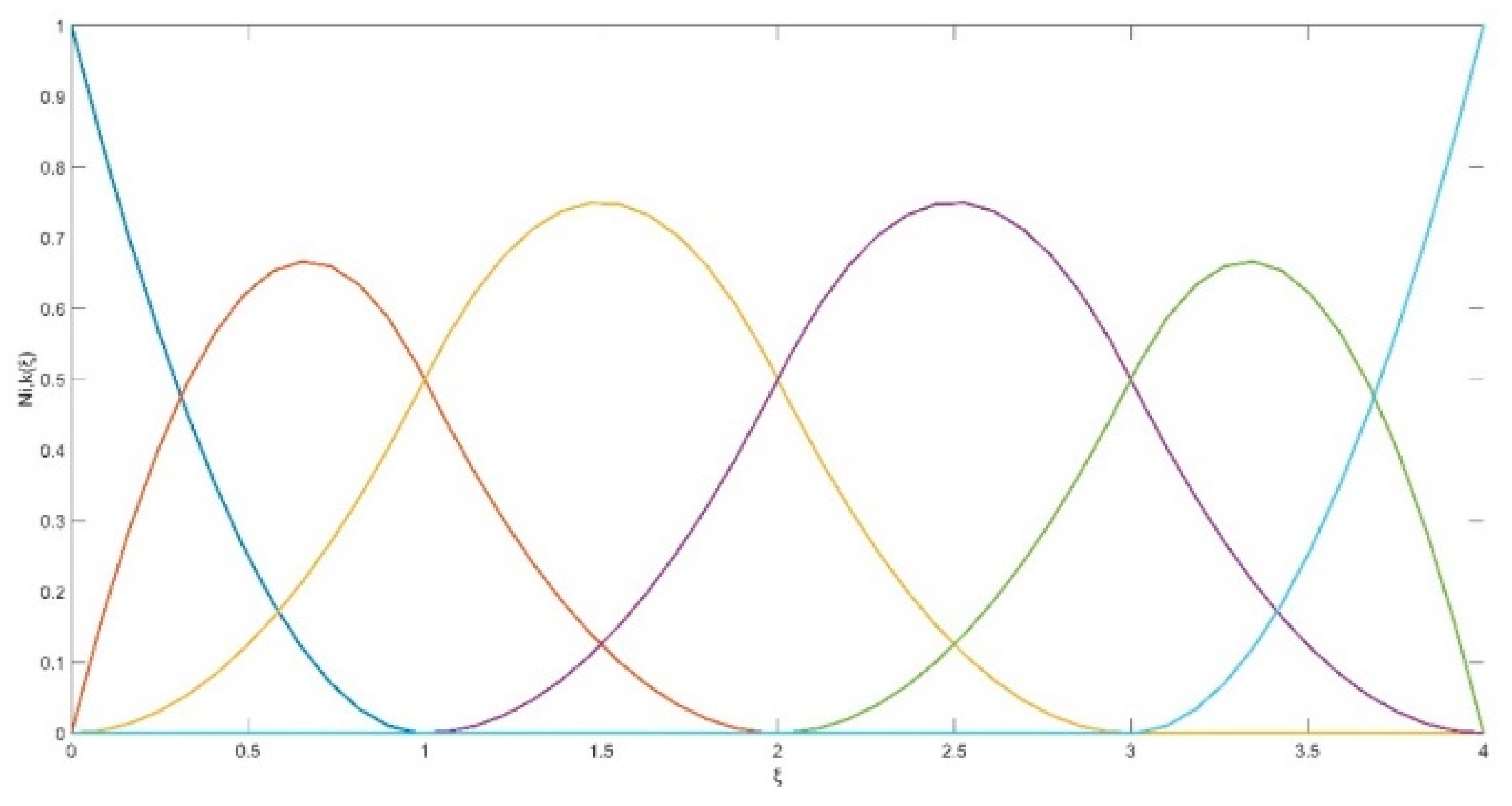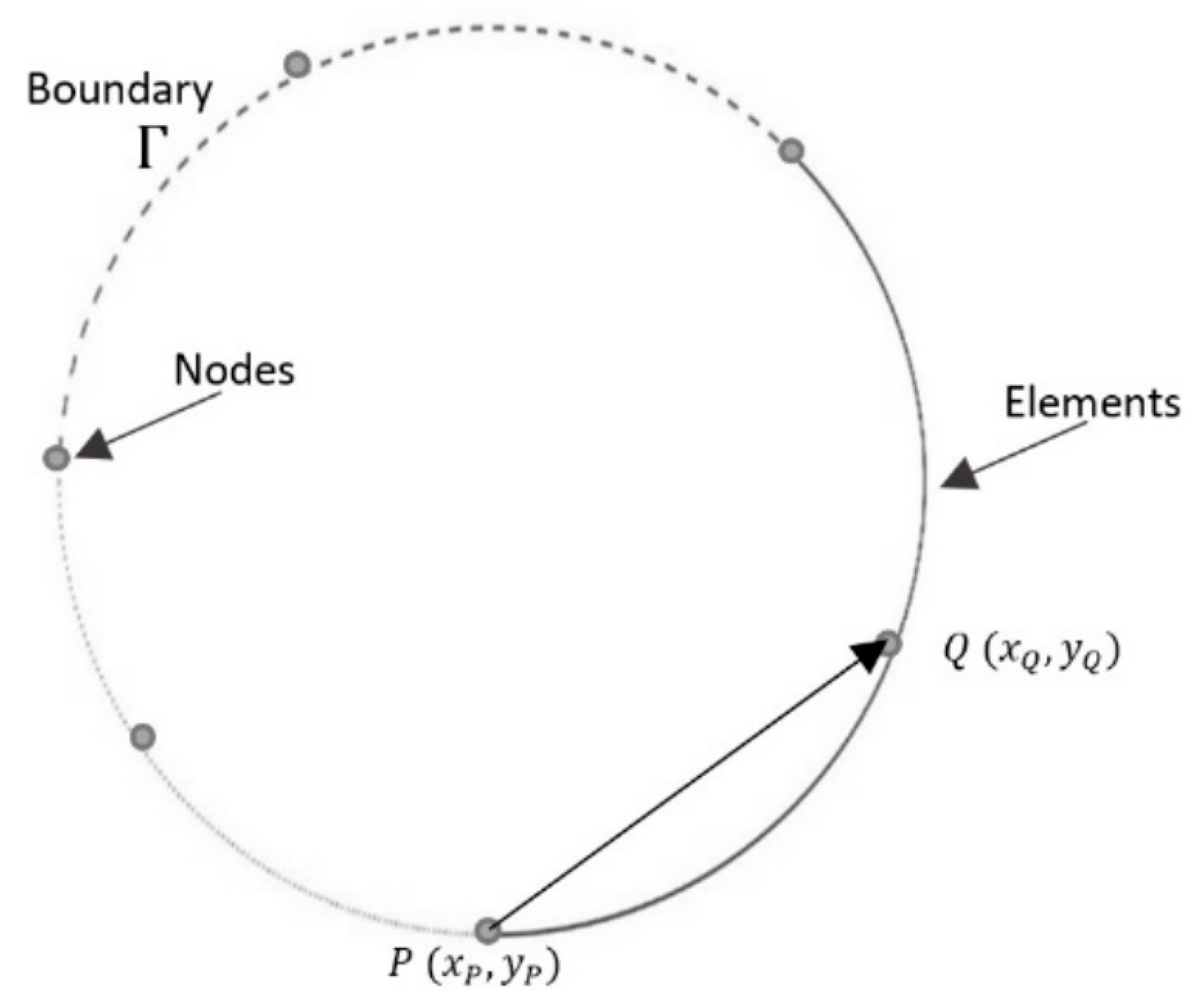The divergence theorem simplifies the continuum mechanics equations solution by modeling only at the boundaries [1]. Such modeling consists of dividing the boundary of the body under analysis into a discrete set of functions, denominated “elements” with nodes, and describing the displacements and tractions by polynomial functions. Since BEM is a consequence of the Betti’s theorem, there are two sets of displacements and tractions. One set is known in advance through entities called traction and displacement kernels, which are valid for any equilibrium geometry. The other set belongs to the body under analysis which is the problem to be solved. Naturally, to obtain a unique solution, boundary conditions such as prescribed tractions and displacements must be applied. The calculated traction and displacement kernels depend on the normal of the surface, the geometric variable, and the interpolation points that describe the boundary. However, the discretization process produces a lack of continuity on the boundary.

An alternative to solve this problem is to use the Non-Uniform Rational B-Splines functions (NURBS) from the CAD model instead of using interpolation functions. This concept was called Isogeometric Analysis (IGA), and it was proposed by Hughes et al. [2] in 2005. Initially, the IGA was used with the FEM framework, but eventually, it was combined with BEM and with the finite cell method (FD).

Simpson et al. [3,4] proposed the Isogeometric Boundary Element Method (IGA-BEM) in 2012 and established the guidelines for combining IGA with BEM, e.g., how the elements are generated using the NURBS knot vector and the NURBS basis functions. They also used the Greville abscissae scheme to get the collocation points and the displacement and traction kernels. Finally, they applied the method to solve the L-plate, the hole-within-an-infinite-plate, and the L-shaped wedge problems.

Takahashi and Matsumoto [5] proposed an IGA-BEM combined with the fast multipole method (FMM), to decrease the control points of the NURBS. They proved that this combination could achieve the same accuracy as the conventional BEM but with fewer degrees of freedom and less computing time. Peake et al. [6] presented an extended IGA-BEM using a partition-of-unity method on NURBS functions; they applied it to solve a two-dimensional Helmholtz problem. Likewise, Scott et al. [7] refined the IGA-BEM, using T-Splines instead of NURBS, to solve linear elastostatic problems; they showed the performance of this method with a patch test and a propeller analysis. Moreover, Lian et al. [8] continued the work of [3,4,7], and they used the T-Splines with IGA-BEM, to optimize the shape of three-dimensional elastic bodies; they chose the control points as design variables to modify the geometry.

The IGA-BEM combination was not only used to reduce the degrees of freedom, changing basis functions, or solving linear problems. For example, Gong and Dong [9] developed a method to calculate the singular integrals on a 3D potential problem and Heltai et al. [10] used IGA-BEM to analyze 3D Stock flows. Peng et al. [11] used a geometric algorithm to propagate fractures, based on the fatigue Paris law, and IGA-BEM to analyze them. Venas and Kvamsdal [12] used IGA-BEM to solve the acoustic scattering problem of a submarine.

The applications of the IGA-BEM in a wide variety of problems have given good results. Nevertheless, the solution depends on calculating the kernels at the interpolation points, restricting the solution domain to the geometry discretization domain. In this work, a methodology based on IGA-BEM is proposed. The method models the body boundary using a single continuous NURBS function thus makes the geometry discretization independent of the evaluation points and separates the kernels calculation from the interpolation functions. These properties allow us to modify the boundary to solve problems like the contact between two bodies.

The mechanical contact has been extensively studied. Johnson [13] described the best-known analytical contact models, such as the Hertz model, the JKR model, and the Bradley model, among others. The Hertz model relates the contact area and the material properties; the JKR model uses the same assumption but adds the interfacial interaction strength; and, finally, the Bradley model considers the external Van der Waals interactions that add load to the contact.

In the numerical methods used in continuum mechanics, the most popular algorithm to analyze the contact is the master–slave. This method consists in projecting the nodes of an elastic body (slave) onto a rigid body (master) when a force is applied. If the slave-node penetrates the body of the master, a force is used in the contact area to return the slave-node to the outer surface of the master. Thereby, the deformation of two bodies in contact is found. This algorithm has been widely used with FEM [14,15,16] and has recently been combined with IGA [17,18,19,20,21,22,23,24]. Nevertheless, the main disadvantage of this method is that applied contact force is not a real force. Additionally, every time this force is used, the contact zone must be found again and verified for penetration. In case penetration is found, another force must be applied, so the algorithm iterates until there is no penetration.

When using BEM, the problem is solved differently [25]. The nodes that are in the contact zone must satisfy two general conditions: there must be continuity between their displacements (not overlapping), and their tractions must be the same but in the opposite direction [25,26,27,28]. As the contact area is not known in advance, the analysis starts with a first contact zone, which is modified until the nodes satisfy the contact conditions. Although the contact is more easily modeled with BEM than with FEM, the analysis draws the disadvantages of BEM, such as the sensitivity to the analysis-points selection that leads to errors in the numerical calculation of the integrals.

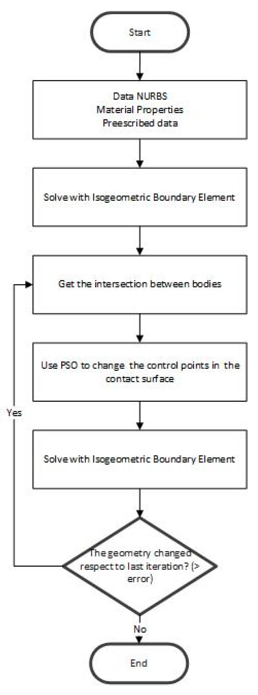
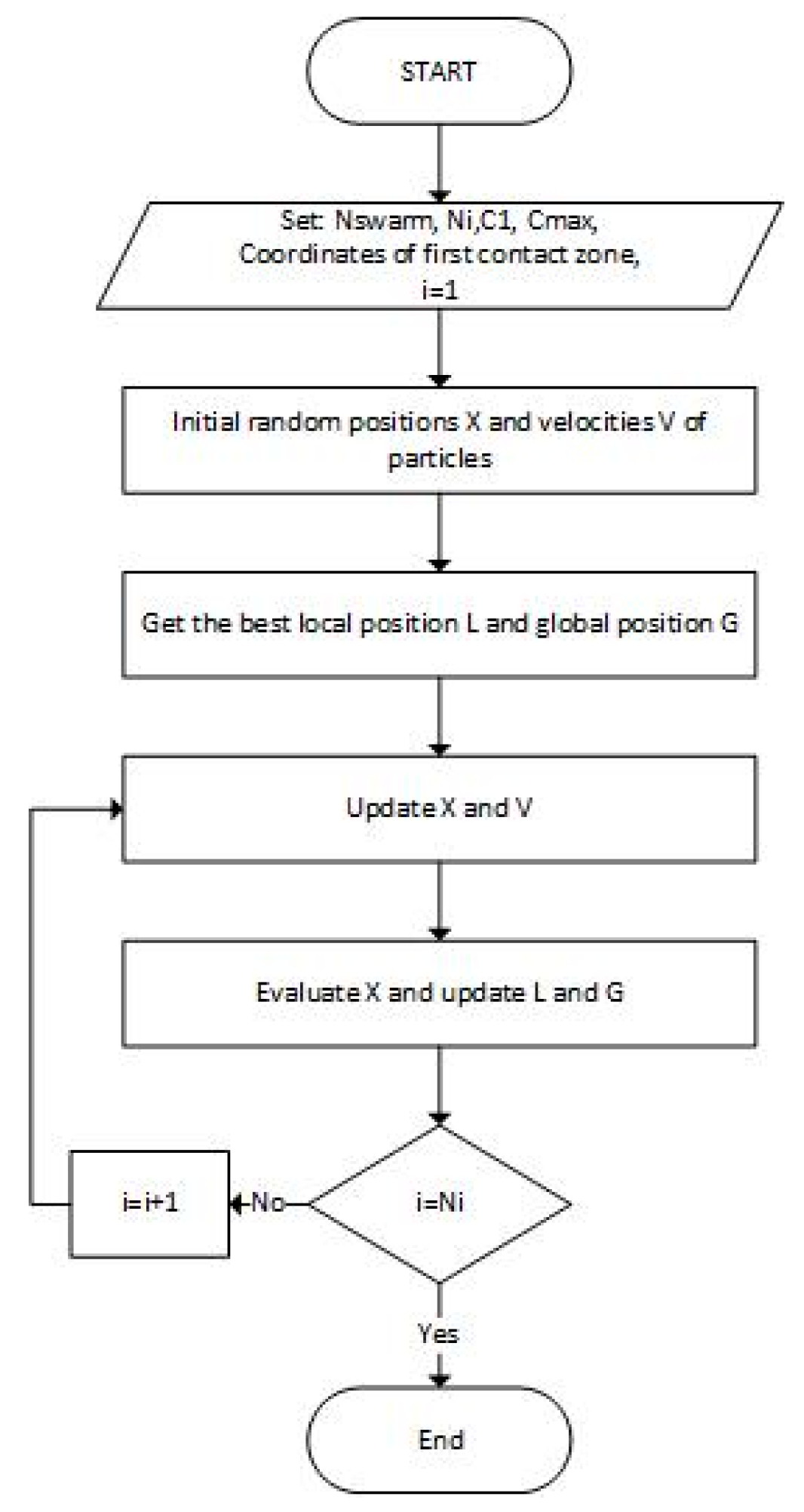
This investigation takes the best features of IGA and BEM to overcome the inconveniences of the conventional BEM. The analysis points of the geometry are separated from the bodies in contact, and the particle swarm optimization (PSO) algorithm is used to find the contact area. In this way, the control points of the NURBS are modified repeatedly, until a correct area is found. With the proposed method, the solution domain is closed (not discrete), by defining the boundary with a single NURBS, and with fewer analysis points in contrast to traditional FEM.

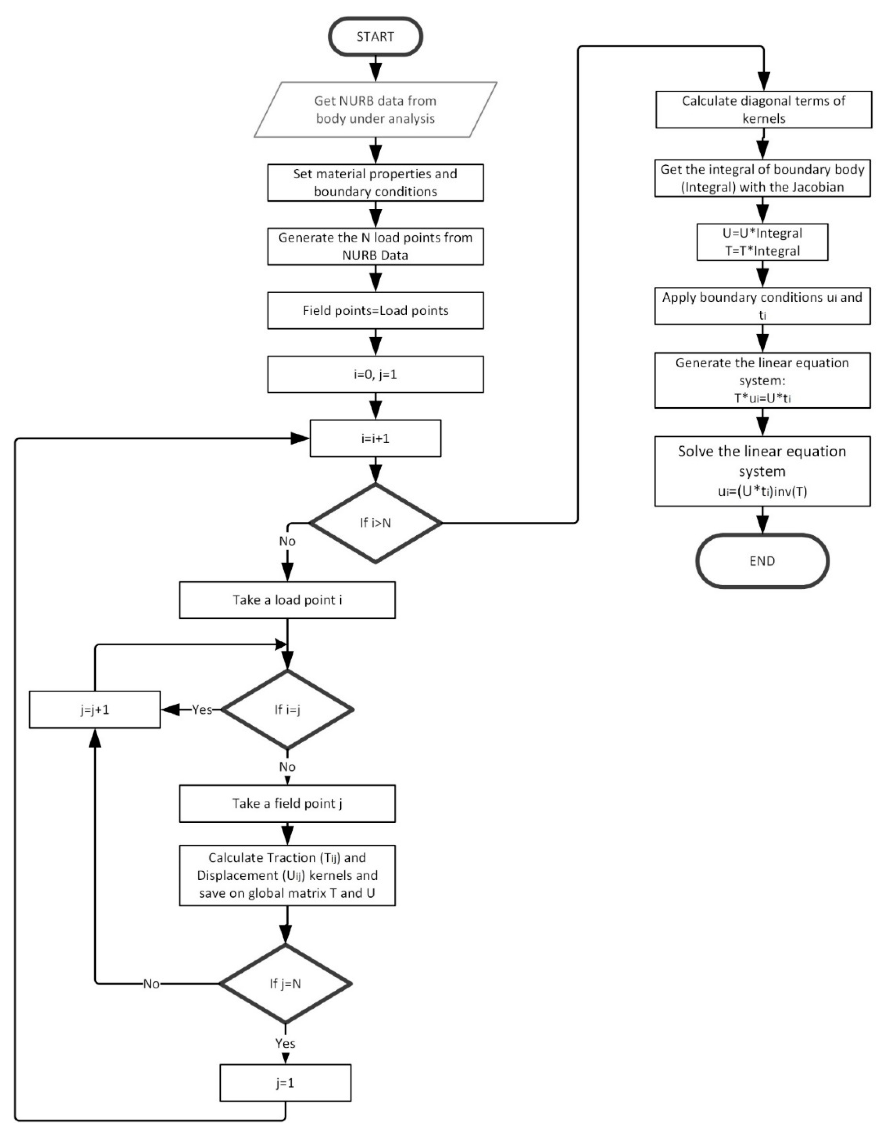
This paper is arranged as follows: Section 2 presents the basis to understand the isogeometric boundary element method, such as the NURBS functions and conventional BEM. Section 3 sets the guidelines to implement the modified IGA-BEM, and later, it details the methodology to be implemented in conjunction with the optimization algorithm. The following section presents the results and properties of the analyzed bodies, as well as a comparison with FEM and BEM. Finally, Section 5 concludes the work and defines future work with the theory presented.

2. Background of Modeling with NURBS and Boundary elements

2.1. Modeling Geometric with NURBS

A NURBS is a parametric curve that can generate lines, conics, and circles accurately. Due to this versatility, it has been widely adopted in computer-aided design programs (CAD). Mathematically, a NURBS curve is defined by Equation (1), where $n$ is the control points number, $\xi$ symbolizes the function parameter, $B$ represents the control points, $w$ the weights, $N$ denotes the B-spline basis functions, Equations (2) and (3), with order $k$ (degree $k-1$). Figure 1 shows the basis function as a function of $\xi$.

$$C\left(\xi \right)=\frac{{{\displaystyle \sum }}_{i=1}^{n+1}{B}_i{w}_i{N}_{i,k}\left(\xi \right)}{{{\displaystyle \sum }}_{i=1}^{n+1}{w}_i{N}_{i,k}\left(\xi \right)}={{\displaystyle \sum }}_{i=1}^{n+1}{B}_i{R}_{i,k}\left(\xi \right),$$

(1)

$$N_{i,1}\left(\xi \right)=\{\begin{array}{l}1{\xi }_i\le \xi <{\xi }_{i+1}\\ 0otherwise\end{array},$$

(2)

$$N_{i,k}\left(\xi \right)=\frac{\left(\xi -{\xi }_i\right)N_{i,k-1}\left(\xi \right)}{{\xi }_{i+k-1}-{\xi }_i}+\frac{\left({\xi }_{i+k}-\xi \right)N_{i+1,k-1}\left(\xi \right)}{{\xi }_{i+k}-{\xi }_{i+1}}$$

(3)

The parameter $\xi$ gets its values from the knot vector $\mathsf{\Xi }=\left[{\xi }_{min}\dots {\xi }_{max}\right]$, which goes from a minimum ${\xi }_{min}$ to a maximum value ${\xi }_{max}$, and its length is $n+1+k$. If $C$ is a closed curve, the values at the ends of the knot vector are repeated $k$ times. The weights, $w,$ allow local control in the shape of the curve; they move the curve closer or farther to the corresponding control point.

The curve continuity can be controlled with the repeated values in the knot vector $\xi$. On the other hand, a NURB curve is $k$ times derivable, and its first derivate is shown in Equation (4).

$$C^{\prime }\left(\xi \right)={{\displaystyle \sum }}_{i=1}^{n+1}{B}_{i}R{\prime }_{i,k}\left(\xi \right),$$

(4)

where:

$$R{\prime }_{i,k}\left(\xi \right)=\frac{w_i{N^{\prime }}_{i,k}\left(\xi \right)}{{{\displaystyle \sum }}_{i=1}^{n+1}{w}_i{N}_{i,k}\left(\xi \right)}-\frac{w_i{N}_{i,k}{{\displaystyle \sum }}_{i=1}^{n+1}{w}_i{N^{\prime }}_{i,k}\left(\xi \right)}{{\left({{\displaystyle \sum }}_{i=1}^{n+1}{w}_i{N}_{i,k}\left(\xi \right)\right)}^2},$$

(5)

In the following sections, we can see that the displacements and tractions are a function of $\xi$ parameter. This causes the method to inherit the properties of the NURBS and accurately represents the body to be analyzed.

2.2. Boundary Element Method

The boundary element method uses Betti’s theorem, which says that the work done by a force system $\left(a\right)$ on the displacements on a system $\left(b\right)$ is equal to the work done by the forces of $\left(b\right)$ on the system displacements of $\left(a\right)$, in a body in equilibrium for two different groups of stresses and strains, Equation (6).

$${{\displaystyle \int }}_V^{}{\sigma }_i^a{\epsilon }_i^b={{\displaystyle \int }}_V^{}{\sigma }_i^b{\epsilon }_i^a,$$

(6)

Using the differential equations of Navier for displacements, the traction definition, and the divergence theorem, Equation (6) turns into (7).

$${{\displaystyle \int }}_{\mathsf{\Gamma }}^{}{t}_i^a{u}_i^{b}dS+{{\displaystyle \int }}_V^{}{f}_i^a{u}_i^{b}dV={{\displaystyle \int }}_{\mathsf{\Gamma }}^{}{t}_i^b{u}_i^{a}dS+{{\displaystyle \int }}_V^{}{f}_i^b{u}_i^{a}dV,$$

(7)

where $t_i^a$ and $t_i^b$ are tractions; $u_i^b$ and $u_i^a$ are displacements; and $f_i^a$ and $f_i^b$ are loads from set $a$ and $b$, respectively. Since the problem to be solved is about solid mechanics, the Kelvin’s solution was applied in the previous equation, to arrive at the Somigliana identity for displacements, Equation (8).

$$u_i\left(p\right)=-{{\displaystyle \int }}_{\mathsf{\Gamma }}^{}{T}_{ij}\left(p,Q\right)u_i\left(Q\right)dS+{{\displaystyle \int }}_{\mathsf{\Gamma }}^{}{U}_{ij}\left(p,Q\right)t_i\left(Q\right)dS+{{\displaystyle \int }}_V^{}{U}_{ij}\left(p,Q\right)f_i\left(q\right)dV,$$

(8)

$T_{ij}$ and $U_{ij}$ represent the traction and displacement kernels from the Kelvin solution, which gives us tractions and displacements on any point of the surface $Q$ when a load is applied to an interior point, $p,$ and is applicable to any geometry. The variables $u_i$, $t_i$, and $f_i$ are the displacements, tractions, and forces to be found. Equations (9) and (10) represent the displacement and traction kernels for the two-dimensional elastostatic problem. These kernels depend on the values of the shear modulus ($\mu$), the Poisson coefficient ($v$), and the distance between the load point $\left(p\right)$ and field point, $Q$, $r\left(p,Q\right)$, described by Equation (11). For each load point and field point, displacement and traction kernels are calculated.

$$U_{ij}\left(p,Q\right)=\frac{1}{8\pi \mu \left(1-v\right)}\left(3-4\upsilon \right)ln\left[\frac{1}{r\left(p,Q\right)}\right]{\delta }_{i,j}+\frac{dr\left(p,Q\right)}{d{x}_i}\frac{dr\left(p,Q\right)}{d{x}_j},$$

(9)

$$\begin{gathered} T_{ij}\left(p,Q\right)=-\frac{1}{8\pi \mu \left(1-v\right)r\left(p,Q\right)}\frac{dr\left(p,Q\right)}{dn}x\left[\left(1-2\nu \right){\delta }_{i,j}+2\frac{dr\left(p,Q\right)}{d{x}_i}\frac{dr\left(p,Q\right)}{d{x}_j}\right] \\ +\frac{1-2v}{4\pi \left(1-v\right)r\left(p,Q\right)}\left[\frac{dr\left(p,Q\right)}{d{x}_j}{n}_i+\frac{dr\left(p,Q\right)}{d{x}_i}{n}_j\right], \end{gathered}$$

(10)

$$r\left(p,Q\right)=\sqrt{{\left(X_p-x_Q\right)}^2+{\left(Y_p-y_Q\right)}^2},$$

(11)

As Equations (8)–(11) have the load point, $p,$ in the interior of body and field point, $Q,$ in the boundary body, it is necessary to move the load point, $p,$ to the boundary. Thus, Equation (7) is transformed into Equation (12), with the absence of body forces:

$$C\left(P\right)u_i\left(P\right)+{{\displaystyle \int }}_{\mathsf{\Gamma }}^{}{T}_{ij}\left(P,Q\right)u_i\left(Q\right)dS={{\displaystyle \int }}_{\mathsf{\Gamma }}^{}{U}_{ij}\left(P,Q\right)t_i\left(Q\right)dS,$$

(12)

where $C\left(P\right)$ is called “Jump Term”. This element moves the internal load point ($p)$ to the boundary, and now the load point is denoted as $P$. The numerical way to solve Equation (12) is to divide the body contour under analysis into “elements”. Each element is composed of “nodes” (Figure 2). Shape functions describe the geometry and displacement and traction variables.

To generate the kernels, a node is taken as the load point, P, and the field point, Q, is generated by each element using shape functions. The diagonal of these kernels corresponds to the point P being equal to the point Q, or P equal to any node of the element. When this happens, the values of the kernels are singular or very close to being singular. A correct approximation of these values is detailed in [25]. Then, a method as the Gaussian quadrature is applied to integrate the kernels on each element. Given these conditions, Equation (12) can be rewritten as follows:

$$\begin{array}{cc}C\left(P\right)u_i\left(P\right)& +{\displaystyle {\displaystyle \sum }_{e=1}^{n_e}{\displaystyle \sum }_{c=1}^3}\left[{{\displaystyle \int }}_{-1}^1{T}_{ij}\left(P,Q\left(\zeta \right)\right)S_c\left(\zeta \right)J^e\left(\zeta \right)d\zeta \right]u_i^e\\ & ={\displaystyle {\displaystyle \sum }_{e=1}^{n_e}{\displaystyle \sum }_{c=1}^3}\left[{{\displaystyle \int }}_{-1}^1{U}_{ij}\left(P,Q\left(\zeta \right)\right)S_c\left(\zeta \right)J^e\left(\zeta \right)d\zeta \right]t_i^e\end{array}$$

(13)

where $\zeta$ is the local coordinate to describe the geometry, $u_i^e$ denotes the displacement, $t_i^e$ the traction at the $e$ element, $n_e$ is the total number of elements, $S$ represents the quadratic shape functions, and $J^e$ denotes the Jacobian element transformation to convert the variables from the boundary $\mathsf{\Gamma }$ to the local coordinate. The integral range $\left[-1,1\right]$ is part of the Gaussian quadrature.

3. Method

3.1. The Proposed Isogeometric Boundary Element Method

The guidelines to use IGA-BEM were established by [3]. In such a way, Equation (13) remains the same, except that the parameter $\xi$ replaces the term $\zeta$ and the shape functions are the B-spline basis functions $N$ with order $k$:

$$\begin{array}{cc}C\left(P\right)u_i\left(P\right)& +{\displaystyle {\displaystyle \sum }_{e=1}^{n_e}{\displaystyle \sum }_{c=1}^k}\left[{{\displaystyle \int }}_{-1}^1{T}_{ij}\left(P,Q\left(\xi \right)\right)N_c\left(\xi \right)J^e\left(\xi \right)d\zeta \right]u_i^e\\ & ={\displaystyle {\displaystyle \sum }_{e=1}^{n_e}{\displaystyle \sum }_{c=1}^k}\left[{{\displaystyle \int }}_{-1}^1{U}_{ij}\left(P,Q\left(\xi \right)\right)N_c\left(\xi \right)J^e\left(\xi \right)d\xi \right]t_i^e\end{array}$$

(14)

However, unlike the method proposed by [3], our model generates the body boundary through a single NURBS, that is, with one “macro-element”. In such a way, it is not necessary to integrate the kernels. Nevertheless, it is required to integrate the Jacobian because the element represents the whole-body contour. The result is the body perimeter.

In addition to the boundary conditions, three sets define the problem to be analyzed:

• Parameter values ξ to get the nodes $P$ and $Q$ on the boundary and generate the values of the kernel.
• The control points ($B$) that define the shape of the body.
• Parameter values $\xi$ to calculate the Jacobian of the macro-element.

The proposed integral boundary equation is given by Equation (15), where $\eta$ represents the $\xi$ values that are used to calculate the Jacobian, which are different from the ξ values to find the $P$ and $Q$ nodes.

$$\begin{array}{cc}C\left(P\left(\xi \right)\right)u_i\left(P\left(\xi \right)\right)& +T_{ij}\left(P\left(\xi \right),Q\left(\xi \right)\right)u_i\left(Q\left(\xi \right)\right){{\displaystyle \int }}_{\mathsf{\Gamma }}^{}J\left(\eta \right)d\eta \\ & =U_{ij}\left(P\left(\xi \right),Q\left(\xi \right)\right)t_i\left(Q\left(\xi \right)\right){{\displaystyle \int }}_{\mathsf{\Gamma }}^{}J\left(\eta \right)d\eta \end{array}$$

(15)

In conventional BEM, the jump term $C$ was calculated indirectly, using rigid body considerations [25]. However, as Simpson et al. [4] described, these considerations are no longer valid, because of the nature of NURBS so the jump term has to be calculated explicitly [29]. However, because the geometry of the body-under-analysis is represented by a single element, the jump term equations are reduced to Equation (16). This matrix only affects the diagonal of the traction kernel when the load point, $P$ coincides with the field point, $Q$.

$$C\left(P\right)=\left[\begin{array}{cc}\frac{1}{2}& 0\\ 0& \frac{1}{2}\end{array}\right],$$

(16)

On the other hand, because the boundary variable, $\mathsf{\Gamma }$, is a function of $\xi$, the term of Jacobian transformation, $J\left(\eta \right)$, is described by the following:

$$J\left(\eta \right)=\frac{d\mathsf{\Gamma }}{d\eta }=\sqrt{{\left(\frac{dx\left(\xi \right)}{d\xi }\right)}^2+{\left(\frac{dy\left(\xi \right)}{d\xi }\right)}^2},$$

(17)

The general flowchart of the isogeometric boundary method proposed is shown in Figure 3. The first step is to read the properties of the material-under-analysis and the NURBS geometry data. That is, the Young modulus ($E$), the Poisson coefficient ($\nu$), the control points ($B$), the knot vector ($\mathsf{\Xi }$), and the curve order ($k)$. Then, a quantity $N$ of load/field points is chosen. The coordinates of the load points on boundary are generated by replacing a value of $\xi$ in the NURBS function.

The next step is to calculate the kernels for each combination of load points, $P,$ and field points, $Q$. Every Kernel is saved in a global matrix of displacement ($U$) and traction ($T$) kernels with size $\left(N\times 2\right)\times \left(N\times 2\right)$. When the load point matches with the field point, the calculation of that traction kernel is skipped and replaced by the jump term of Equation (14). In the case of the displacement kernel, a tolerance is added or subtracted from the field point, to prevent the term (1/r) from going to infinity. The obtained global kernels are multiplied by the integral of the body boundary Equation (17); if a more exact value of the integral is desired, more $\xi$ values may be added and may be different from the $\xi$ values for the load and field points.

Following the flowchart in Figure 3, the next step is to apply the boundary conditions to generate a unique solution. Thus, it is necessary to accommodate the unknown variables, either displacements or tractions, on the left side, and those known on the right side, to arrive at the system of equations of the form $Ax=b$. The kernels would be the matrix “A,” and the displacement and the tractions prescribed would be “$b$”. Finally, by solving the equation system, the unknown values of displacement and tractions are obtained.

The next equations represent some additional elements to compute the kernels; the $\frac{dy\left(\xi \right)}{d\xi }$ and $\frac{dx\left(\xi \right)}{d\xi }$ terms are gotten by Equation (5).

$$\frac{dr}{dx}=\frac{X_Q\left(\xi \right)-X_P\left(\xi \right)}{r\left(P\left(\xi \right),Q\left(\xi \right)\right)},$$

(18)

$$\frac{dr}{dy}=\frac{Y_Q\left(\xi \right)-Y_P\left(\xi \right)}{r\left(P\left(\xi \right),Q\left(\xi \right)\right)},$$

(19)

$$n_x=\frac{dx}{dn}=\frac{1}{J\left(\xi \right)}\left[\frac{dy\left(\xi \right)}{d\xi }\right],$$

(20)

$$n_y=\frac{dy}{dn}=-\frac{1}{J\left(\xi \right)}\left[\frac{dx\left(\xi \right)}{d\xi }\right],$$

(21)

$$\frac{dr}{dn}=\frac{dr}{dx}\frac{dx}{dn}+\frac{dr}{dy}\frac{dy}{dn},$$

(22)

3.2. Application: Contact between Two Bodies

The contact is analyzed by following the unilateral equations described in the Sognirini problem (contact between a rigid and an elastic body) and the Winkler–Westergaard problem (contact between elastic bodies). One of these equations, Equation (23), establishes that the normal displacements of one body, with respects to the other, are less than or equal to zero; therefore, there is no penetration between both bodies.

$$u\left(x\right)·{n|}_{\mathsf{\Gamma }}\le 0$$

(23)

If the contact is analyzed with the proposed modified IGA-BEM, there would be two bodies that share a common area that, after applying a load, reach equilibrium, as observed in Equations (24) and (25):

$$\begin{array}{cc}{u}_i\left(p\right)& +{{\displaystyle \int }}_{{\mathsf{\Gamma }}_1}^{}{T}_{ij}\left(p,Q\right)u_i\left(Q\right)dS+{{\displaystyle \int }}_{{\mathsf{\Gamma }}_{AB}}^{}{T}_{ij}\left(p,Q\right)u_i\left(Q\right)dS\\ & ={{\displaystyle \int }}_{{\mathsf{\Gamma }}_1}^{}{t}_i\left(Q\right)U_{ij}\left(p,Q\right)dS+{{\displaystyle \int }}_{{\mathsf{\Gamma }}_{AB}}^{}{t}_i\left(Q\right)U_{ij}\left(p,Q\right)dS\end{array}$$

(24)

$$\begin{array}{cc}{u}_i\left(p\right)+& {{\displaystyle \int }}_{{\mathsf{\Gamma }}_2}^{}{T}_{ij}\left(p,Q\right)u_i\left(Q\right)dS+{{\displaystyle \int }}_{{\mathsf{\Gamma }}_{AB}}^{}{T}_{ij}\left(p,Q\right)u_i\left(Q\right)dS\\ & ={{\displaystyle \int }}_{{\mathsf{\Gamma }}_2}^{}{t}_i\left(Q\right)U_{ij}\left(p,Q\right)dS+{{\displaystyle \int }}_{{\mathsf{\Gamma }}_{AB}}^{}{t}_i\left(Q\right)U_{ij}\left(p,Q\right)dS\end{array}$$

(25)

${\mathsf{\Gamma }}_1$ and ${\mathsf{\Gamma }}_2$ represent the boundaries of body 1 and body 2, respectively, that are not in contact. ${\mathsf{\Gamma }}_{AB}$ represents the region of the common boundary between the two bodies, that is, the contact zone, (Figure 4). Since this region is unknown, an optimization algorithm will be applied to find it. The flowchart of the contact methodology can be seen in Figure 5.

The first stage of the flowchart consists of executing the complete diagram of Figure 3. The second stage is to find the intersection between the two bodies (points $A$ and $B$). If these elements had the same Young’s modulus and the applied force is large enough, the nature of the IGA-BEM would create penetration between both bodies. This situation is not real; what physically happens is that these elements are deformed without penetration. The deformation value depends on the applied force and the materials properties.

The third stage is to modify the control points, using the PSO algorithm to create new body geometries with the same area as the originals but fixing the contact area. To ensure that the contact area is correct, the same load is reapplied. If the contact zone changes, then the cycle is repeated; if it does not change, or the difference between one iteration and another is minimal, then the contact algorithm is stopped. The details of the PSO algorithm are described in the next section.

3.3. The Particle Swarm Optimization

An optimization algorithm is a method to find the maximum or minimum of a given function. For the contact problem of Figure 4, the objective function is shown in Equation (26), where $I$ corresponds to the perimeter of the deformed body, and $I_{or}$ corresponds to the body perimeter before applying the load. The algorithm varies the NURBS control points that define the bodies, and the contact zone is assumed to be a straight line (Figure 6).

$$I_{or}-I=0$$

(26)

There is a wide variety of optimization algorithms, but those algorithms based on nature stand out. For example, the genetic algorithms, the particle swarm optimization, the ant colony optimization, and the differential evolution, among others. In this paper, the particle swarm algorithm was chosen because it is easy to implement and has fast convergence [30].

The PSO is inspired by how animal herds behave. The flowchart of this method is shown in Figure 7. The first step is to set the population size or “swarm” ($N_{swarm}$). Each “individual” of the community has a set of optimization variables or design variables that represent their position ($X$). These elements move in the solution space by adjusting their speeds ($V$). However, the individual speed depends on their previous position and speed values. Moreover, it depends on the best individual location ($L$) and the best position of all individuals ($G$). The algorithm runs until the maximum number of iterations ($N_i$) is reached. The last best global position values correspond to the design optimized variables.

The function to be optimized is the initial perimeter of the bodies, and the design variables are the control points ($B$) that are outside of the contact zone. The next position $X_i$ and velocity $V_i$ values of each particle are calculated by using Equations (27) and (28), respectively, where the best particle position is $L_i$, and the best position of all particles is $G_N$.

$$V_{i+1}=C_1{V}_i+C_{max}rand\left(0,1\right)\left(L_i-X_i\right)+C_{max}rand\left(0,1\right)\left(G_N-X_i\right),$$

(27)

$$X_{i+1}=X_i+V_i$$

(28)

To update the best local and global values, the function to be optimized must be analyzed. This means the perimeter of the body for each $X_i$ value must be calculated. The elements of $X_i$ are the new control points. If the perimeter is higher or less than the original, then a penalization is applied by adding or subtracting an amount from the obtained perimeter value, Equations (29) and (30), where k represents a proportional constant to the difference between the value of $I$ and $I_{or}$. To update the best local position, $L_i$, the penalized $I$ is compared with the best saved local perimeter; if the new $I$ value is better than the saved, the best local position $L_i$ is updated. The same procedure is done to update the best global location.

$$ifI>I_{or}\Rightarrow I=I+abs\left(kI\right)$$

(29)

$$ifI<I_{or}\Rightarrow I=I-\left(kI\right)$$

(30)

4. Results

The methodology described in Section 3.1 was programmed to solve a plane strain problem, and its results were compared with FEM and the conventional BEM. Figure 8 represent the problem: A load was applied on the top of the cylinder, and the opposite side was fixed. Being a plane problem, it is not necessary to create the cylinder model; instead, only the cross-section is required. The cylinder dimensions and the material properties can be found in

Table 1. Material properties of the body under analysis.

$\mathbf{Load}\mathit{P}$	$\mathbf{Young}\text{’}\mathbf{s}\mathbf{Modulus}\mathit{E}$	$\mathbf{Poisson}\text{’}\mathbf{s}\mathbf{Coefficient}\mathit{v}$	Circle Diameter
$-4500N,$ Y component	$2\times {10}^{11}\mathrm{Pa}$	$0.3$	6 mm

, likewise the load value. The results of this problem are presented in Section 4.1, Section 4.2 and Section 4.3.

The proposed modified IGA-BEM was used to analyze the contact between two cylinders. The contact problem was also analyzed as a plane strain problem. Both cylinders have the material properties defined in Table 1. The load was applied as shown in Figure 9, and a displacement restriction was placed at the bottom of the cylinders. A symmetric behavior in the deformation is assumed as the contact zone is the same for both circles. The results of this problem are presented in Section 4.4 and Section 4.5.

4.1. Plane Strain Problem-Solve with FEM

A commercial FEM software was used to solve the problem presented in Figure 8. First, a load was set on the upper side, and the load was distributed between two neighboring nodes. Next, displacement restrictions on the nodes were added on the opposite side. A fine mesh was made, generating 2566 nodes and 827 elements (Figure 10a). The result of this problem is shown in Figure 10b.

4.2. Plane Strain Problem-Solve with Conventional BEM

The strain problem of Figure 8 was solved with a program based on BEM and the algorithm proposed by [25]. To solve the problem, the following data was used: 71 nodes, 36 elements distributed on the boundary (Figure 11a), 6 integration points for Gaussian Quadrature, quadratic shape functions to describe tractions and displacements, and the data from Table 1. The result can be found in Figure 11b. To generate the internal displacements, 13 internal points were chosen using the guidelines described by [25].

4.3. Plane Strain Problem Solve with the Isogeometric-Boundary Integral Element Method Proposed

To create the circle with NURBS, the curve order, the control points, and the knot vector were first calculated. Those values are shown in

Table 2. Data to create NURBS curve from the plane strain problem.

Knot Vector	$\mathsf{\Xi }=\left[0,0,0,1,1,2,2,3,3,4,4,4\right]$
Control points	$B=\left[00;30;33;36;06;-36;-33;-30;00\right]$
Weight vector	$W=\left[1,\frac{\sqrt{2}}{2},1,\frac{\sqrt{2}}{2},1,\frac{\sqrt{2}}{2},1,\frac{\sqrt{2}}{2}1\right]$
Curve order	$k=3$

. As seen in Section 3.2, the load points have to be generated on the boundary. Therefore, 24 values of $\xi$ were chosen, to generate the coordinates of the load/field points, using Equation (1).

Table 3. Data to analyze the plane strain problem with the proposed method.

Load/field points number	$24$
Elements number	$1$
Control points number (for NURBS geometry)	$9$
Jacobian points number	$50$

specifies the additional elements to use the proposed method. The used load/field points and control points are shown in Figure 12a. The deformed cylinder is shown in Figure 12b. Like the conventional BEM, the internal displacements are calculated by adding internal points.

4.4. Contact Problem Solve with Hertz Theory

According to [31], the width of the rectangular contact area between two cylinders can be found by Equation (28) when they have the same elasticity modulus ($E=E_1=E_2$) and the same Poisson coefficient ($v=0.3)$. In Equation (31), $p$ represents the load per unit length ($P/L)$, $K_D$ is the relative curvature ($\raisebox{1ex}{$D_1\cdot D_2$}\!\left/ \!\raisebox{-1ex}{$D_1+D_2$}\right.$) and, $b$ is the width of the rectangular of contact area. More detailed information about Hertz theory can be found at [13]. The length of the cylinder is 100 mm.

$$b=2.15\sqrt{\frac{p{K}_D}{E}}$$

(31)

If the values described in Table 1 and in the previous paragraph are substituted in Equation (31), the width of the contact area is $b=.056\mathrm{mm}$. Following Hertz’s theory, the maximum Hertzian contact pressure, the maximum shear stress, and its depth can be found. These values are shown in

Table 4. Results obtained with the Hertz theory.

Width of the contact area	$0.056\mathrm{mm}$
Maximum Hertzian contact pressure	$1024.4\mathrm{MPa}$
Maximum shear stress	$308\mathrm{MPa}$
Depth of maximum shear stress	$0.022\mathrm{mm}$

.

4.5. Contact Problem Solve with FEM

The contact problem was also solved with FEM software. The parameters used in the simulation are described in

Table 5. Parameters to solve the contact problem with FEM.

Element order	Quadratic
Contact type	Frictionless
Behavior	Symmetric
Method to solve the contact	Augmented Lagrange
Detection method	Nodal-normal to target
Nodes number	2184
Elements number	696

. A fine mesh was chosen to obtain greater results’ precision (Figure 13a). To avoid penetration between the bodies, the augmented Lagrange method was chosen. The behavior of this algorithm was briefly described in the introduction section. Figure 13b shows the deformed bodies, and the color map represents the displacements in Y. The maximum deformation is located in the load application area. The contact zone has a length of approximately 0.65 mm, as seen in Figure 14.

4.6. Contact Problem Solved with Proposed IGA-BEM.

To use the proposed contact algorithm from Section 3.2, some control points were added near to the common point (0, 0). The NURBS data to create the two cylinders in contact are in

Table 6. Data to create NURBS curve from the plane strain problem.

Knot Vector	$\mathsf{\Xi }=\left[0,0,0,1,1,2,2,3,3,4,4,5,5,6,6,6\right]$
Control points, upper cylinder	$B=[00;0.26250;0.52090.0456;30.04827;33;36;06;-36;-33;$ $-30.4827;-0.52090.0456;-0.26250;00]$
Control points, lower cylinder	$B=[00;0.26250;0.5209-0.0456;3-0.04827;3-3;3-6;0-6;$ $-3-6;-3-3;-3-0.4827;-0.5209-0.0456;-0.26250;00]$
Weight vector	$W=\left[1,0.9962,1,0.7660,1,0.7071,1,0.7071,1,0.7660,1,0.9962,1\right]$
Curve order	$k=3$

. As seen, weights were also changed to maintain the circular shape of the cylinders.

Table 7. Data to analyze the contact problem with the proposed method.

Load/field points number	$24$
Elements number	$1$
Control points number (for NURBS geometry)	$13$
Jacobian points number	$50$

specifies the data to solve the problem with the proposed IGA-BEM. The load points were generated by selecting 24 values of $\xi$ distributed between the minimum and maximum value of this variable. Unlike the problem in Section 4.3, the control points increased 9–13 (Figure 6). Finally, the number of points to calculate the Jacobian was set to 50, to obtain a more accurate value; however, this value is only calculated once. Figure 15 shows the two cylinders deformed after applying the load. Figure 16 is a close-up to the contact area and shows the interference between the bodies.

Table 8. Data to run the PSO algorithm.

Generation number	$300$
Swarm size	$25$
$C_1$	$0.8$
$C_{max}$	$1.62$

details the input parameters of the optimization algorithm. The values of C1 and C2 were set according to the recommendation of Clerc [31].

Figure 17 shows the bodies in contact without penetration, after having implemented the algorithm proposed in Section 3.2. As can be seen, in Figure 18, the contact area is a straight line. This zone has a length of approximately 62 mm.

5. Discussion

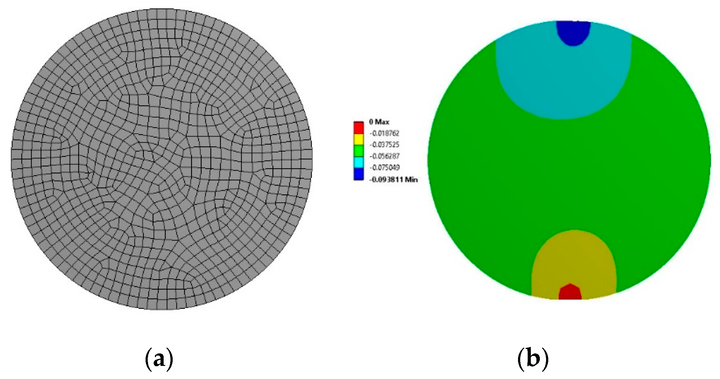
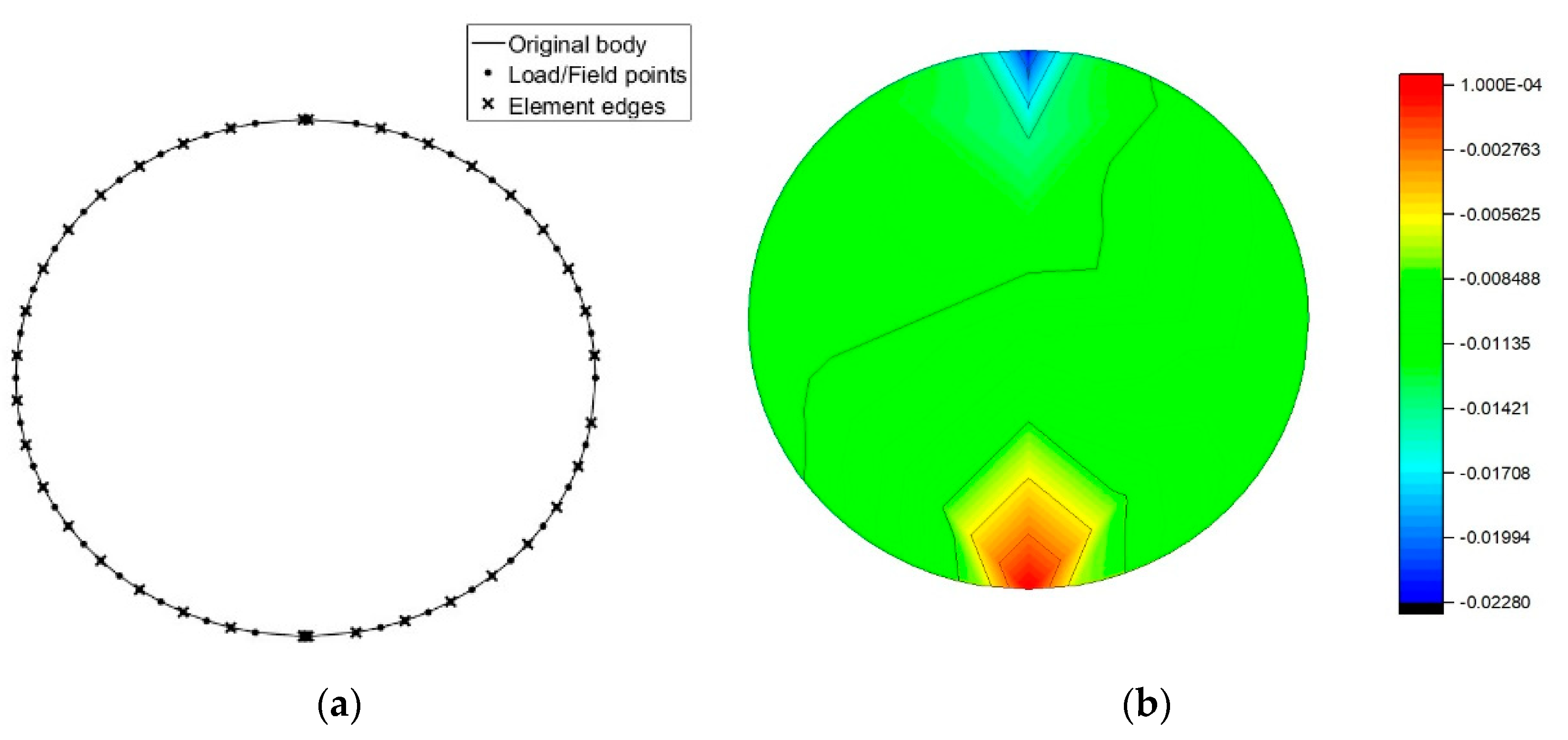
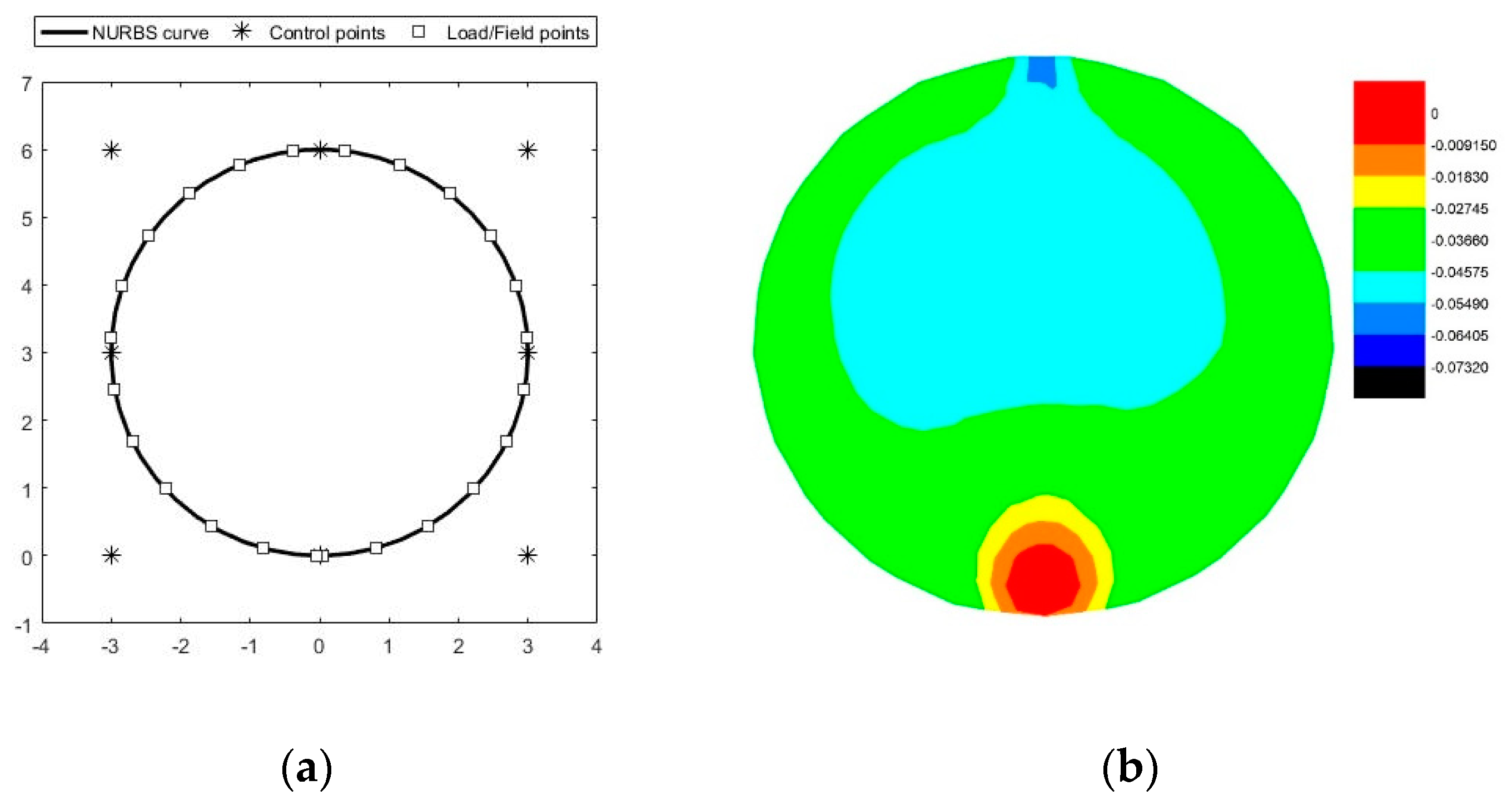
As seen in the previous section, the three methods generated similar deformed bodies when solving the plane strain problem. With a fine mesh, the maximum displacement in the Y-axis with FEM was $-0.094\mathrm{mm}$, while with the conventional BEM, it was $-0.023\mathrm{mm}$, and with the proposed IGA-BEM method, it was $-0.073\mathrm{mm}$. The maximum displacement was seen where the P load was applied. To solve the problem, the FEM software used 2566 nodes or analysis points, while BEM used 71 analysis points, and the proposed IGA-BEM used 24 analysis points. Internal points were added in BEM and proposed IGA-BEM to obtain the internal displacements. In contrast, given the nature of FEM, the analysis did not require adding additional points.

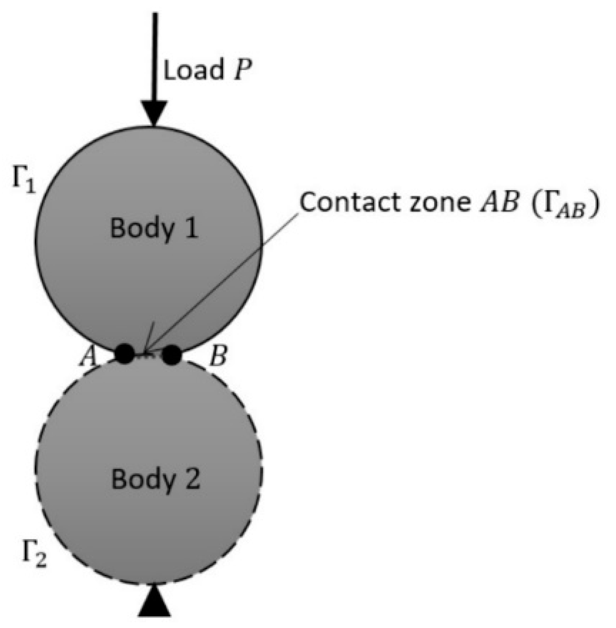
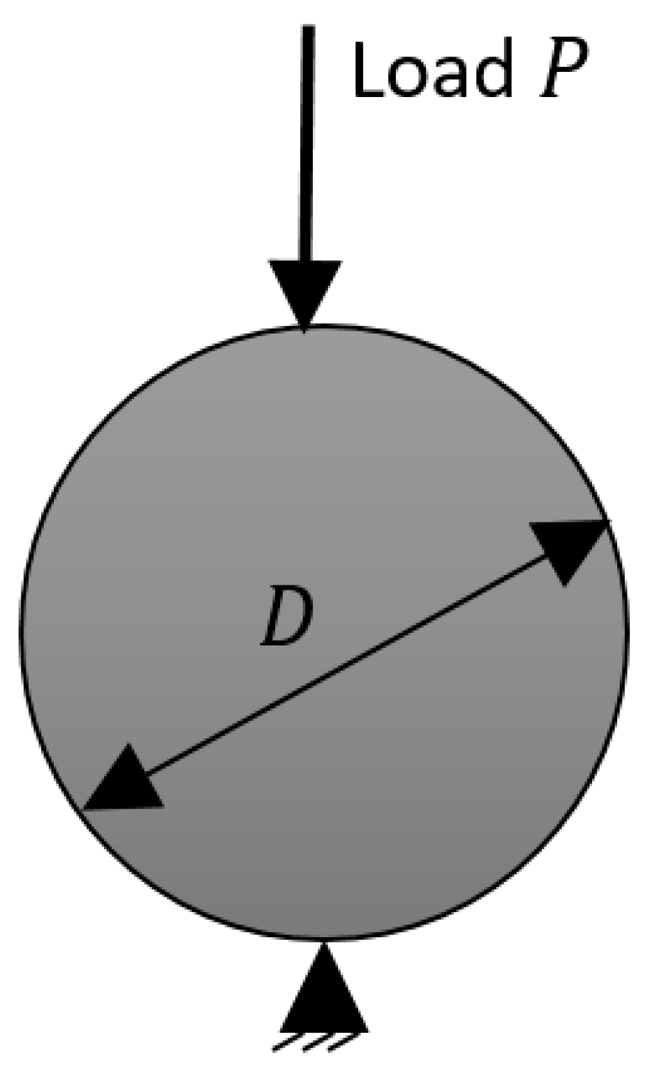
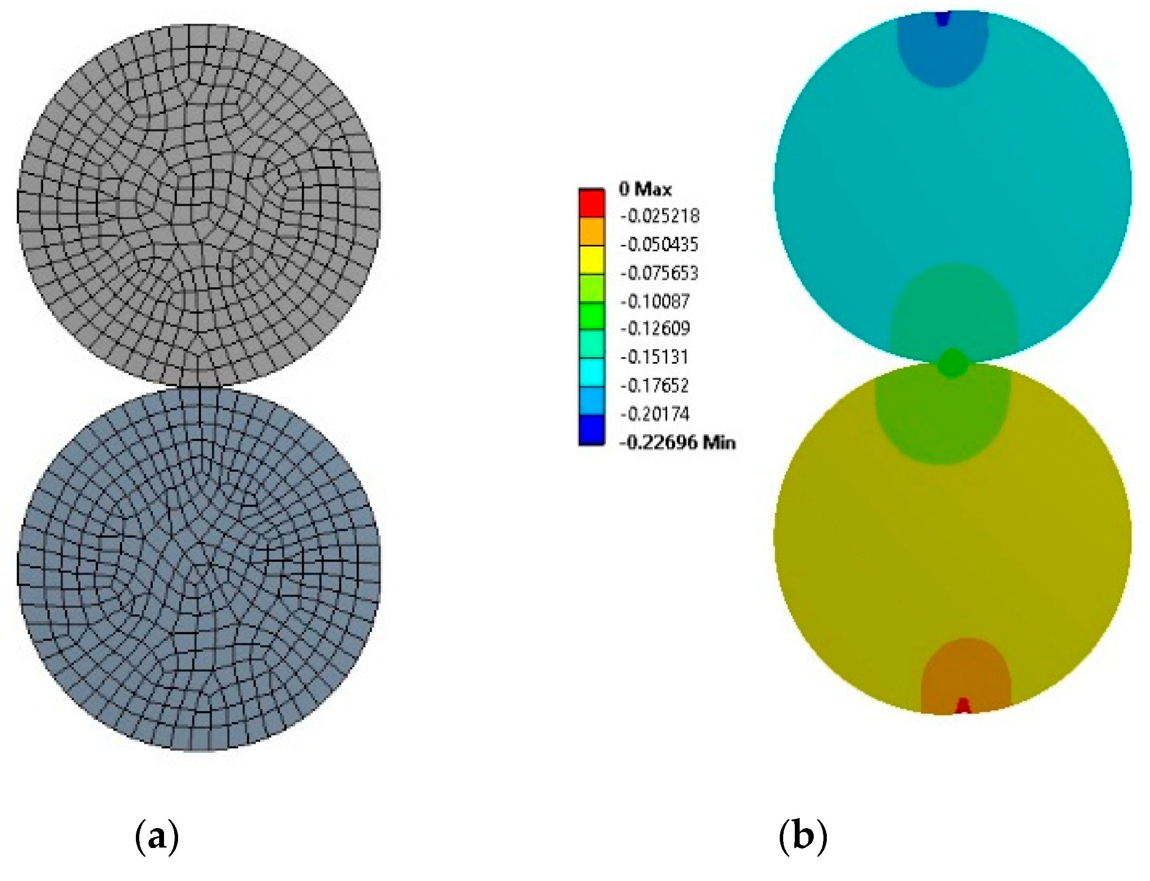
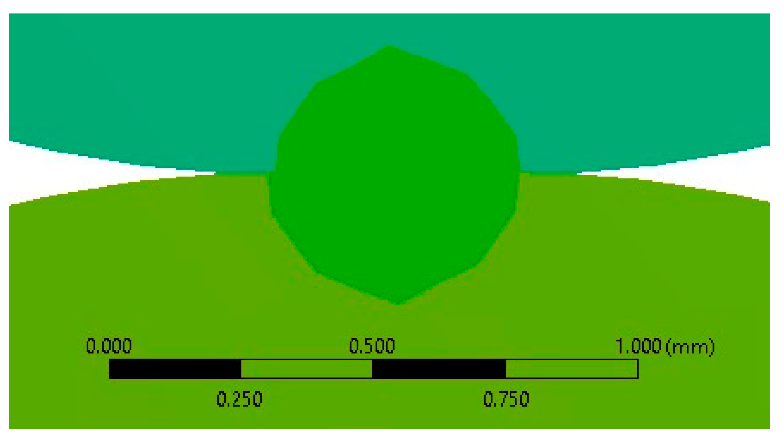
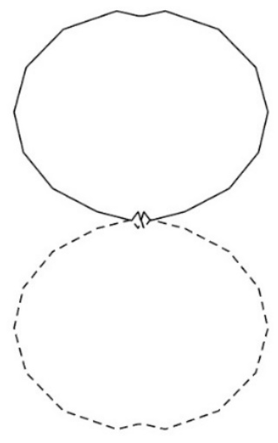
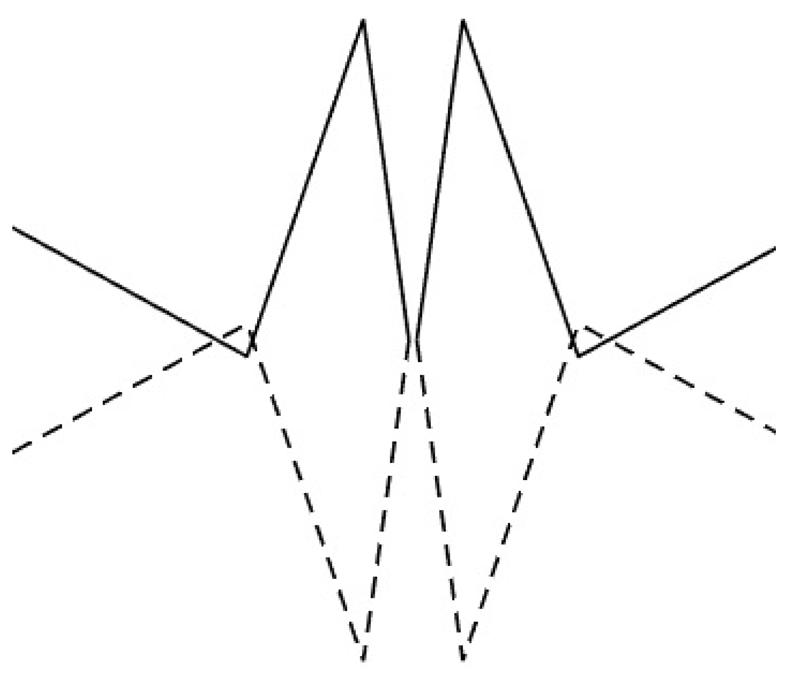
Regarding the contact problem,

Table 9. Comparison of contact area widths.

Method	Contact Area Width (mm)	Variation with Respect to the Analytical Method	DOF to Solve the Problem
Analytical (Hertz model)	$0.56$	$0$	-
FEM	$0.65$	$16\%$	4368
Proposed IGA-BEM of contact	$0.62$	$11\%$	48

shows a comparison of the contact area widths obtained with the Hertz model, the FEM software, and the proposed IGA-BEM of contact. Taking the analytical solution as a reference, the error obtained with FEM was 16%, while the proposed method was 10%. In both cases, interference between the bodies was eliminated after applying the load. With FEM, the problem was solved by using a total of 2184 nodes, equivalent to 4368 Degrees of Freedom (DOF). With the proposed IGA-BEM, the problem was solved using 24 analysis points (48 DOF), but the control points that define the bodies’ shape increased 9–13. On the other hand, the deformed figure was obtained after the PSO algorithm converged in a value gap.

Although the proposed method solves the problems with fewer degrees of freedom compared to FEM, it requires more robustness to avoid sensitivity problems in the calculation of $n_x$ and $n_y$; The same issue was also observed with the conventional BEM.

6. Conclusions

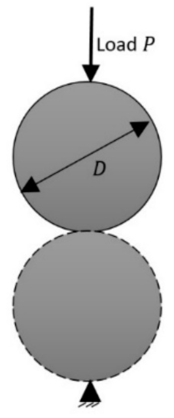
The proposed IGA-BEM got consistent results, while solving the problem of Figure 8, compared to those obtained from the proven methods FEM and BEM. Although the displacement values were different, the deformation generated was similar in all three methods. However, fewer degrees of freedom were required in proposed IGA-BEM, because a single NURBS was used to model the completed body. Moreover, the load/field points used in the conventional BEM were separated from the points, to represent the geometry.

Regarding the nonlinear contact problem, the contact-zone widths obtained with FEM and with the proposed contact method varied 16% and 10%, respectively, compared to the one obtained analytically, with the Hertz method. Nevertheless, the DOF used by FEM to solve the contact problem were 4368, while the proposed method only used 48 DOF.

Decreasing degrees of freedom is very significant, for example, when solving multiphysics problems, where it is required to invert matrices. Furthermore, as seen in [32], the propagation error is tied to the size of the matrix: The more elements the matrix has, the higher the error.

Although the results are promising, future work is required to prove that the methodology is valid in other situations where displacements are not symmetrical or additional factors, such as friction, are considered.

References

1. Rizzo, F.J. An integral equation approach to boundary value problems of classical elastostatics. Q. Appl. Math. 1967, 25, 83–95. [Google Scholar] [CrossRef] [Green Version]
2. Hughes, T.J.R.; Cottrell, J.A.; Bazilevs, Y. Isogeometric analysis: CAD, finite elements, NURBS, exact geometry and mesh refinement. Comput. Methods Appl. Mech. Eng. 2005, 194, 4135–4195. [Google Scholar] [CrossRef] [Green Version]
3. Simpson, R.N.; Bordas, S.P.A.; Trevelyan, J.; Rabczuk, T. A two-dimensional Isogeometric Boundary Element Method for elastostatic analysis. Comput. Methods Appl. Mech. Eng. 2012, 209, 87–100. [Google Scholar] [CrossRef]
4. Simpson, R.N.; Bordas, S.P.A.; Lian, H.; Trevelyan, J. An isogeometric boundary element method for elastostatic analysis: 2D implementation aspects. Comput. Struct. 2013, 118, 2–12. [Google Scholar] [CrossRef] [Green Version]
5. Takahashi, T.; Matsumoto, T. An application of fast multipole method to isogeometric boundary element method for Laplace equation in two dimensions. Eng. Anal. Bound. Elem. 2012, 36, 1766–1775. [Google Scholar] [CrossRef]
6. Peake, M.J.; Trevelyan, J.; Coates, G. Extended isogeometric boundary element method (XIBEM) for two-dimensional Helmholtz problems. Comput. Methods Appl. Mech. Eng. 2013, 259, 93–102. [Google Scholar] [CrossRef] [Green Version]
7. Scott, M.A.; Simpson, R.N.; Evans, J.A.; Lipton, S.; Bordas, S.P.A.; Hughes, T.J.R.; Sederberg, T.W. Isogeometric boundary element analysis using unstructured T-splines. Comput. Methods Appl. Mech. Eng. 2013, 254, 197–221. [Google Scholar] [CrossRef] [Green Version]
8. Lian, H.; Kerfriden, P.; Bordas, S.P.A. Shape optimization directly from CAD: An isogeometric boundary element approach using T-splines. Comput. Methods Appl. Mech. Eng. 2017, 317, 1–41. [Google Scholar] [CrossRef]
9. Gong, Y.P.; Dong, C.Y. An isogeometric boundary element method using adaptive integral method for 3D potential problems. J. Comput. Appl. Math. 2017, 319, 141–158. [Google Scholar] [CrossRef]
10. Heltai, L.; Arroyo, M.; DeSimone, A. Nonsingular isogeometric boundary element method for Stokes flows in 3D. Comput. Methods Appl. Mech. Eng. 2014, 268, 514–539. [Google Scholar] [CrossRef] [Green Version]
11. Peng, X.; Atroshchenko, E.; Kerfriden, P.; Bordas, S.P.A. Isogeometric boundary element methods for three dimensional static fracture and fatigue crack growth. Comput. Methods Appl. Mech. Eng. 2017, 316, 151–185. [Google Scholar] [CrossRef] [Green Version]
12. Venås, J.V.; Kvamsdal, T. Isogeometric boundary element method for acoustic scattering by a submarine. Comput. Methods Appl. Mech. Eng. 2020, 359, 112670. [Google Scholar] [CrossRef]
13. Johnson, K.L. Contact Mechanics; Cambridge University Press: Cambridge, UK, 1987. [Google Scholar]
14. Di Capua, D.; Agelet de Saracibar, C. A direct elimination algorithm for quasi-static and dynamic contact problems. Finite Elem. Anal. Des. 2015, 93, 107–125. [Google Scholar] [CrossRef] [Green Version]
15. Cavalieri, F.J.; Cardona, A. Numerical solution of frictional contact problems based on a mortar algorithm with an augmented Lagrangian technique. Multibody Syst. Dyn. 2015, 35, 353–375. [Google Scholar] [CrossRef]
16. Neto, D.M.; Oliveira, M.C.; Menezes, L.F. Surface Smoothing Procedures in Computational Contact Mechanics. Arch. Comput. Methods Eng. 2017, 24, 37–87. [Google Scholar] [CrossRef]
17. Guo, Y.; Ruess, M.; Gürdal, Z. A contact extended isogeometric layerwise approach for the buckling analysis of delaminated composites. Compos. Struct. 2014, 116, 55–66. [Google Scholar] [CrossRef]
18. De Lorenzis, L.; Wriggers, P.; Zavarise, G. A mortar formulation for 3D large deformation contact using NURBS-based isogeometric analysis and the augmented Lagrangian method. Comput. Mech. 2012, 49, 1–20. [Google Scholar] [CrossRef]
19. Matzen, M.E.; Cichosz, T.; Bischoff, M. A point to segment contact formulation for isogeometric, NURBS based finite elements. Comput. Methods Appl. Mech. Eng. 2013, 255, 27–39. [Google Scholar] [CrossRef]
20. Temizer, I.; Abdalla, M.M.; Gürdal, Z. An interior point method for isogeometric contact. Comput. Methods Appl. Mech. Eng. 2014, 276, 589–611. [Google Scholar] [CrossRef] [Green Version]
21. Temizer, I.; Wriggers, P.; Hughes, T.J.R. Contact treatment in isogeometric analysis with NURBS. Comput. Methods Appl. Mech. Eng. 2011, 200, 1100–1112. [Google Scholar] [CrossRef]
22. Temizer, I.; Hesch, C. Hierarchical NURBS in frictionless contact. Comput. Methods Appl. Mech. Eng. 2016, 299, 161–186. [Google Scholar] [CrossRef] [Green Version]
23. De Lorenzis, L.; Evans, J.A.; Hughes, T.J.R.; Reali, A. Isogeometric collocation: Neumann boundary conditions and contact. Comput. Methods Appl. Mech. Eng. 2015, 284, 21–54. [Google Scholar] [CrossRef]
24. Dimitri, R.; De Lorenzis, L.; Scott, M.A.; Wriggers, P.; Taylor, R.L.; Zavarise, G. Isogeometric large deformation frictionless contact using T-splines. Comput. Methods Appl. Mech. Eng. 2014, 269, 394–414. [Google Scholar] [CrossRef]
25. Becker, A.A. The Boundary Element Method in Engineering: A Complete Course; Mc-Graw Hill International: Cambridge, UK, 1992; ISBN 0-07-707439-4. [Google Scholar]
26. Wu, J.-J.; Lin, Y.J. Boundary element analyses on the adhesive contact between an elastic sphere and a rigid half-space. Eng. Anal. Bound. Elem. 2017, 74, 61–69. [Google Scholar] [CrossRef]
27. Vallepuga Espinosa, J.; Foces Mediavilla, A. Boundary element method applied to three dimensional thermoelastic contact. Eng. Anal. Bound. Elem. 2012, 36, 928–933. [Google Scholar] [CrossRef]
28. Nguyen, V.T.; Hwu, C. Boundary element method for two-dimensional frictional contact problems of anisotropic elastic solids. Eng. Anal. Bound. Elem. 2019, 108, 49–59. [Google Scholar] [CrossRef]
29. Guiggiani, M. A self-adaptive co-ordinate transformation for efficient numerical evaluation of general boundary element integrals. Int. J. Numer. Methods Eng. 1988, 26, 1683–1684. [Google Scholar] [CrossRef]
30. Camacho-Gutiérrez, S.V.; Jáuregui-Correa, J.C.; Dominguez, A. Optimization of Excitation Frequencies of a Gearbox Using Algorithms Inspired by Nature. J. Vib. Eng. Technol. 2019, 7, 551–563. [Google Scholar] [CrossRef]
31. Young, W.C.; Budynas, R.G.; Sadegh, A.M. Roark’s Formulas for Stress and Strain; McGraw-Hill: New York, NY, USA, 2002; Volume 7. [Google Scholar]
32. Lefebvre, M.; Keeler, R.K.; Sobie, R.; White, J. Propagation of errors for matrix inversion. Nucl. Instrum. Methods Phys. Res. Sect. A Accel. Spectrometers Detect. Assoc. Equip. 2000, 451, 520–528. [Google Scholar] [CrossRef] [Green Version]
Figure 1. Basis function for k = 3 and Ξ = [ 0   0   0   1   2   3   4   4   4   ] .
Applsci 10 02345 g001
Figure 2. Nodes and elements using in the conventional BEM.
Applsci 10 02345 g002
Figure 3. General flowchart of the proposed IGA-BEM.
Applsci 10 02345 g003
Figure 4. Contact zone between bodies.
Applsci 10 02345 g004
Figure 5. Flowchart to analyze contact with the proposed IGA-BEM.
Applsci 10 02345 g005
Figure 6. Contact zone and control points.
Applsci 10 02345 g006
Figure 7. Flowchart of PSO.
Applsci 10 02345 g007
Figure 8. Cylinder under load P and a fixed point.
Applsci 10 02345 g008
Figure 9. Cylinders in contact under load P and a fixed point.
Applsci 10 02345 g009
Figure 10. Cylinder under load P solve with FEM. (a) Mesh used in FEM software. (b) Cylinder deformed solved with FEM software; the plot colors represent the displacement in Y direction.
Applsci 10 02345 g010
Figure 11. Cylinder under load P solve with conventional BEM. (a) Analysis points used as field/load points and element edges to solve the problem with BEM. (b) Cylinder under load; the plot colors represent the displacements in Y direction.
Applsci 10 02345 g011
Figure 12. Cylinder under load P solved with the proposed IGA-BEM. (a) Load/field points used as analysis point, and control points used to generate the NURB curve. (b) Cylinder deformed; the plot colors represent the displacements in Y direction.
Applsci 10 02345 g012
Figure 13. Contact between two bodies analyzed with FEM. (a) Mesh used in FEM software. (b) Contact between two bodies analyzed with FEM software; the plot colors represent the displacement in Y direction.
Applsci 10 02345 g013
Figure 14. Close-up to the contact area between two bodies analyzed with FEM.
Applsci 10 02345 g014
Figure 15. Contact between two bodies analyzed with proposed IGA-BEM.
Applsci 10 02345 g015
Figure 16. Close-up to the contact area between two bodies analyzed with proposed IGA-BEM before optimization.
Applsci 10 02345 g016
Figure 17. Contact between two bodies analyzed with the IGA-BEM and the optimization proposed.
Applsci 10 02345 g017
Figure 18. Close-up to the contact area between two bodies analyzed with the IGA-BEM and the optimization proposed.
Applsci 10 02345 g018