A Combined Visualization Method for Multivariate Data Analysis. Application to Knee Kinematic and Clinical Parameters Relationships

Abstract

This paper aims to analyze the correlation structure between the kinematic and clinical parameters of an end-staged knee osteoarthritis population. The kinematic data are a set of characteristics derived from 3D knee kinematic patterns. The clinical parameters include the answers of a clinical questionnaire and the patient’s demographic characteristics. The proposed method performs, first, a regularized canonical correlation analysis (RCCA) to evaluate the multivariate relationship between the clinical and kinematic datasets, and second, a combined visualization method to better understand the relationships between these multivariate data. Results show the efficiency of using different and complementary visual representation tools to highlight hidden relationships and find insights in data.

1. Introduction

Data visualization and multivariate data analysis are an active and current research area in applied statistics, engineering, and data mining. They become an increasingly popular area for displaying and exploring complex and multidimensional data involving several application domains (finances, engineering, and healthcare) in which the relationships between many attributes are of vital interest [1,2]. Multivariate statistical methods are designed to simultaneously analyze data sets of multiple variables and are used to model different forms of relationships among variables.

Biomedical data are usually multidimensional and multimodal [3,4]. For that reason, biomedical data mining research requires the use of multivariate analysis to study the association between various variables whilst controlling for several other variables [5]. Multivariate data visualization is therefore strongly motivated to investigate the interrelationships between different data attributes, to identify, cluster, and correlate the underlying data.

In this paper, we investigate the multivariate relationship between knee kinematics and clinical parameters of patients who suffer from end-stage knee osteoarthritis (OA). The kinematic parameters are first derived from a gait analysis, which is one of the promising assessment tools used in orthopedic research for assessing changes in gait of knee OA patients. Gait analysis, including joint kinematics, kinetics, and dynamic EMG data, provides objective and shareable data. This analysis was initially introduced to clinical practice [6] and is one of the specific methods used to gain useful clinical knowledge on the functional status of the join.

Clinical gait analysis is the process of recording and interpreting biomechanical measurements during gait in order to assist in treatment decision-making for groups of patient with gait dysfunction. Thereby, appropriateness of gait analysis prescription and reliability of data obtained are required in the clinical environment. Clinical gait analysis [7] is performed to allow help in the clinical decision making regarding treatment options including the conservative (non-surgical) or surgical treatment. This is based on one or more diagnosis, assessment, monitoring, and prediction. The most common use is for assessment of patients with a known condition prior to planning treatment [8]. According to Baker [6], the usefulness of clinical gait analysis is now widely accepted and there is now a growing demand for this service. The principal clinical domains of the clinical use of gait analysis are: cerebral palsy, stroke, traumatic brain injury, and lower limb amputation. At present, the clinical gait analysis operates in the classification of a group of patients in specific normal or abnormal patterns of movement with particular impairments of body structure and function. Certain criteria must be fulfilled for gait analysis to be useful in the clinical evaluation of patients, the biomechanical parameters must (1) correlate with the functional capacity of the patient, (2) supply additional, more relevant information than the clinical examination, (3) be accurate and repeatable, (4) result from a test which does not alter the natural performance of the patient, and (5) be interpreted by experienced clinicians [6].

In this context of clinical gait analysis, we propose a technical approach that aims at understanding the association between kinematic measurements and clinical data related to the functional status of the patient. In that way, we will be able to identify some gait characteristics associated with clinical measures that should therefore be considered in the treatment decision process.

Many studies analyze the correlation between kinematic features of gait waveform data and clinical parameters by using bivariate analysis [9,10]. Through some bivariate analysis results, gait and biomechanical changes were associated with knee OA severity levels [11,12]. For the end-staged knee OA patients, correlations were found between kinematics features in the sagittal plane and clinical measures such as symptoms during specific tasks, active range of motion, functional test, and clinical frailty scale [10]. Associations were also found between radiographic features and clinical functional status in severe knee OA [13], and between physical activity level and physical performance for patients with end-stage knee osteoarthritis [14]. However, a multivariate analysis is more adapted to investigate the correlation between kinematic and clinical parameters, because it can evaluate the strength of the relationship considering the complexity of biomechanical data [15] and the interrelationships of the two datasets of parameters, as we showed in our previous study [16].

The aim of this paper is to investigate visually the multivariate correlation between two datasets of kinematic measurements and clinical parameters which are measured during specific tasks and functional tests of patients with end-stage knee OA.

2. Materials and Methods

This study performs, first, a regularized canonical correlation analysis (RCCA) to evaluate the multivariate relationship between clinical and kinematic datasets and, second, a combined visualization method to better understand the relationships between these multivariate data.

Univariate and multivariate statistical techniques are two important methods for understanding and analyzing detailed statistical data. Univariate analysis is the precursor to multivariate analysis, and knowledge of the first is needed to understand the second. Univariate correlation analysis is a simple linear correlation in which the relationship between two variables depends on their constant. Multivariate (canonical) correlation analysis (CCA) is used to explain as much as possible the variance derived from the relationships between two groups of numerical variables in a reduced dimension space. The CCA may suffer from instability. That is why a regularized approach of CCA (RCCA) is investigated in this study.

2.1. Regularized Canonical Correlation Analysis (RCCA)

Canonical correlation analysis (CCA) is the multivariate extension of linear correlation analysis that has been described by Hotelling [17]. The main purpose of CCA is the exploration of sample correlations between two sets of variables whose roles in the analysis are strictly symmetric and are observed on the same individual. The CCA is currently used in some disciplines such as ecology [18,19], biology [20,21], hydrology [22,23], and health [16].

In this study, the CCA is performed to investigate the relationships between two sets of variables, namely the kinematic $\mathit{X}$ and clinical $\mathit{Y}$ datasets, measured on the same individuals.

Let $\mathit{X}\left(X_1,X_2,\dots ,X_p\right)$ and $\mathit{Y}\left(Y_1,Y_2,\dots ,Y_q\right)$ be two matrices of standardized variables (centered and reduced) of order $n\times p$ and $n\times q$, respectively. Where $n=143$ OA patients, $p=69$ kinematic variables and $q=42$ clinical variables. The CCA consists in finding in stepwise optimization problem two vectors ${\mathit{A}}_{\mathit{s}}$ and ${\mathit{B}}_{\mathit{s}}$, for $s=1,\dots ,min\left(p,q\right)$, that maximize the correlations between the linear combinations:

$${\mathit{U}}_{\mathit{s}}=a_1^s{X}_1+a_2^s{X}_2+\dots +a_p^s{X}_p=\mathit{X}{\mathit{A}}_{\mathit{s}}$$

(1)

$${\mathit{V}}_{\mathit{s}}=b_1^s{Y}_1+b_2^s{Y}_2+\dots +b_q^s{Y}_q=\mathit{Y}{\mathit{B}}_{\mathit{s}}$$

(2)

assuming that vectors $A_s$ and $B_s$ are normalized so that var($U_s$) = var($V_s$) = 1.

In other words, the problem consists in solving

$${\rho }_s=\mathit{c}\mathit{o}\mathit{r}\left({\mathit{U}}_{\mathit{s}},{\mathit{V}}_{\mathit{s}}\right)=\underset{{\mathit{A}}_{\mathit{s}},{\mathit{B}}_{\mathit{s}}}{\max } \mathit{c}\mathit{o}\mathit{r}\left(\mathit{X}{\mathit{A}}_{\mathit{s}},\mathit{Y}{\mathit{B}}_{\mathit{s}}\right)$$

(3)

subject to var($\mathit{X}{\mathit{A}}_{\mathit{s}}$) = var($\mathit{Y}{\mathit{B}}_{\mathit{s}}$) = 1 and the restriction that $cor\left({\mathit{U}}_{\mathit{t}},{\mathit{U}}_{\mathit{s}}\right)=cor\left({\mathit{V}}_{\mathit{t}},{\mathit{V}}_{\mathit{s}}\right)=0$ for $1\le t<s$. ${\rho }_s$ is called the canonical correlation, ${\mathit{U}}_{\mathit{s}}$ and ${\mathit{V}}_{\mathit{s}}$ (${\mathit{U}}_{\mathit{t}}$ and ${\mathit{V}}_{\mathit{t}}$, respectively), are known as the canonical variate vectors. The coefficient vectors ${\mathit{A}}_{\mathit{s}}$ and ${\mathit{B}}_{\mathit{s}}$ are known as the canonical weights (or loadings), canonical vectors, or canonical coefficients. The Pillai’s trace test is used for the statistical significance of the canonical correlation model [24,25].

The CCA may suffer from instability. Indeed, when the variable related to a data set are highly correlated (nearly collinear), the sample correlation matrix tends to be ill-conditioned and its inverse unreliable. In that case, a regularized approach of CCA (RCCA) solves the instability of the loadings due to multicollinearity by adding a regularization term on the diagonal of the ill-conditionned matrices, i.e., the covariance matrices [20]. A regularization step in the computations of classical CCA consists in the regularization of the covariance matrices $S_{XX}$ and $S_{YY}$ of $\mathit{X}$ and $\mathit{Y}$, respectively, by adding a multiple number of the corresponding identity matrices:

$$S_{XX}\left({\lambda }_1\right)= S_{XX} + {\lambda }_1{I}_p$$

(4)

$$S_{YY}\left({\lambda }_2\right) = S_{YY}+ {\lambda }_2{I}_q$$

(5)

where ${\lambda }_1$ and ${\lambda }_2$ are non-negative numbers (also called regularization terms) imposed to the diagonal of the covariance matrices such that $S_{XX}\left({\lambda }_1\right)$ and $S_{YY}\left({\lambda }_1\right)$ becomes regularized and nonsingular [20]. The regularization terms, ${\lambda }_1$ and ${\lambda }_2$, associated to each dataset are chosen by cross-validation in order to maximize the first canonical correlation.

2.2. RCCA Cross-Correlation Matrix

The $\mathit{X}$ and $\mathit{Y}$ variables are projected onto a low-dimensional space. Let $s=2$ for the chosen dimension to adequately account for the data correlation. The projection is done on the equiangular vector $W_k$ between the canonical variates ${\mathit{U}}_{\mathit{k}}$ and ${\mathit{V}}_{\mathit{k}}$ ($k=1,2$) represented by ${\mathit{W}}_{\mathit{k}}=\left({\mathit{U}}_{\mathit{k}}+{\mathit{V}}_{\mathit{k}}\right)/2$. In CCA, the variables $X$ and $Y$ are symmetrically analyzed, and it is clear that $\mathit{W}$ are the closest (most correlated) variable to $\mathit{X}$ and $\mathit{Y}$ [26]. To identify and grouping each pair of strongly correlated variables, we use a standard measure to quantify the most important cross-correlations, which is based on the scalar product of the $\mathit{X}$ and $\mathit{Y}$ coordinates on the canonical axes ${\mathit{W}}_{\mathit{k}}$ ($k=1,2$).

Let $\mathit{x}$ and $\mathit{y}$ be the coordinates of the variables $\mathit{X}$ and $\mathit{Y}$, respectively, on the axes $W_1$ and $W_2$, which are the correlations between the variables $\mathit{X}$ (or $\mathit{Y}$) and ${\mathit{W}}_{\mathit{k}}$: $\mathit{x}=\left(\mathit{c}\mathit{o}\mathit{r}\left(\mathit{X},{\mathit{W}}_{\mathbf{1}}\right);\mathit{c}\mathit{o}\mathit{r}\left(\mathit{X},{\mathit{W}}_{\mathbf{2}}\right)\right)$ and $\mathit{y}=\left(\mathit{c}\mathit{o}\mathit{r}\left(\mathit{Y},{\mathit{W}}_{\mathbf{1}}\right);\mathit{c}\mathit{o}\mathit{r}\left(\mathit{Y},{\mathit{W}}_{\mathbf{2}}\right)\right)$. The Matrix $Z={\mathit{x}\mathit{y}}^{\prime }$ ($0\le Z\le 1$) represents an approximation of the cross-correlation score of $\mathit{X}$ and $\mathit{Y}$, using the scalar product between the variables vectors $\mathit{x}$ and $\mathit{y}$. Indeed, the scalar product is defined as the product of the two vectors lengths and their cosine angle: $Z=\parallel \mathit{x}\parallel \parallel \mathit{y}\parallel cos\theta \left(\mathit{x},\mathit{y}\right)$, where $\theta \left(\mathit{x},\mathit{y}\right)$ is the angle between $\mathit{x}$ and $\mathit{y}$. Therefore, the cross-correlation value should be stronger or weaker depending on the lengths and the angles between the variable vectors; the higher the norm of the projected vectors, the stronger their relationship. Furthermore, the variables $\mathit{X}$ and $\mathit{Y}$ have a strong relationship if they are projected in the same (or opposite) direction, so the cosine is close to 1 (resp. of −1).

2.3. Graphical Visualizations

Different graphical representations to visualize and interpret the results of RCCA are investigated: (1) the correlation variable representation that has the ability to identify the between-correlated clusters of each type of variables and (2) the cross-correlation variable representation which provides additional visual inferences, allowing the combination between a selected subsets of the between-correlated clusters that have the higher correlation. The relevance of relationships can be controlled by tuning a threshold of correlation. The combined visualization of these graphical outputs is important and immediately becomes imminent for clustering the most relevant correlated variables and highlighting omitted knowledge about multivariate correlation.

2.3.1. Representation of Canonical Variable Correlation

The correlation variable representation is performed using a biplot to visualize the variables of two different types. This representation discerns the structure of correlation between the two sets of variables $\mathit{X}$ and $\mathit{Y}$. For a given pair $\left(t,s\right)$ of axes such that $1\le t<s$, variables plots can be considered with respect to ${\mathit{W}}_{\mathit{t}}$ and ${\mathit{W}}_{\mathit{s}}$. The correlation is between the two types of projected variables $\mathit{X}$ and $\mathit{Y}$ onto the space spanned by the first components retained in the analysis (${\mathit{W}}_{\mathbf{1}}$ and ${\mathit{W}}_{\mathbf{2}}$). The correlation points of each variables are visualized as a scatter plot on the axes ${\mathit{W}}_{\mathbf{1}}$ and ${\mathit{W}}_{\mathbf{2}}$. Therefore, the correlation variable is represented by a correlation circle plot [20] by plotting the coordinates vectors of $\mathit{x}$ and $\mathit{y}$ in a 2-dimensional cartesian coordinate system. The closer the distance to the circle of radius $1$, the stronger is the correlation between the variables. The cosine angle between any two segments related to each points represents the nature of correlation (negative, positive, or null) between two variables.

2.3.2. Cross-Correlation Variable Representation

As a simple graphical display of a correlation matrix, heatmap, and relevance network are two visualizations of the cross-correlation matrix $Z$ that give an alternative view of the biplot and shows clearly the patterns of negative/positive correlations.

• Visualizing the cross-correlation variable by the heatmap.

Heatmap for one matrix is a 2-dimensional visualization of the correlation matrix with rows and/or columns reordered according to some hierarchical clustering method to identify interesting patterns. Generated dendrograms (tree diagrams) from clustering are added to the image to represent the arrangement of the clusters. The nature of the correlation between variables (positive, negative, strong, or weak) is represented by color, whereas the proximity between correlated variables is represented by the dendrogram. Usually, we try to find well-visible rectangles of the same color corresponding to the long sections of the dendrograms to identify the clustered correlations [27].

• Visualizing the cross-correlation variable by the relevance network.

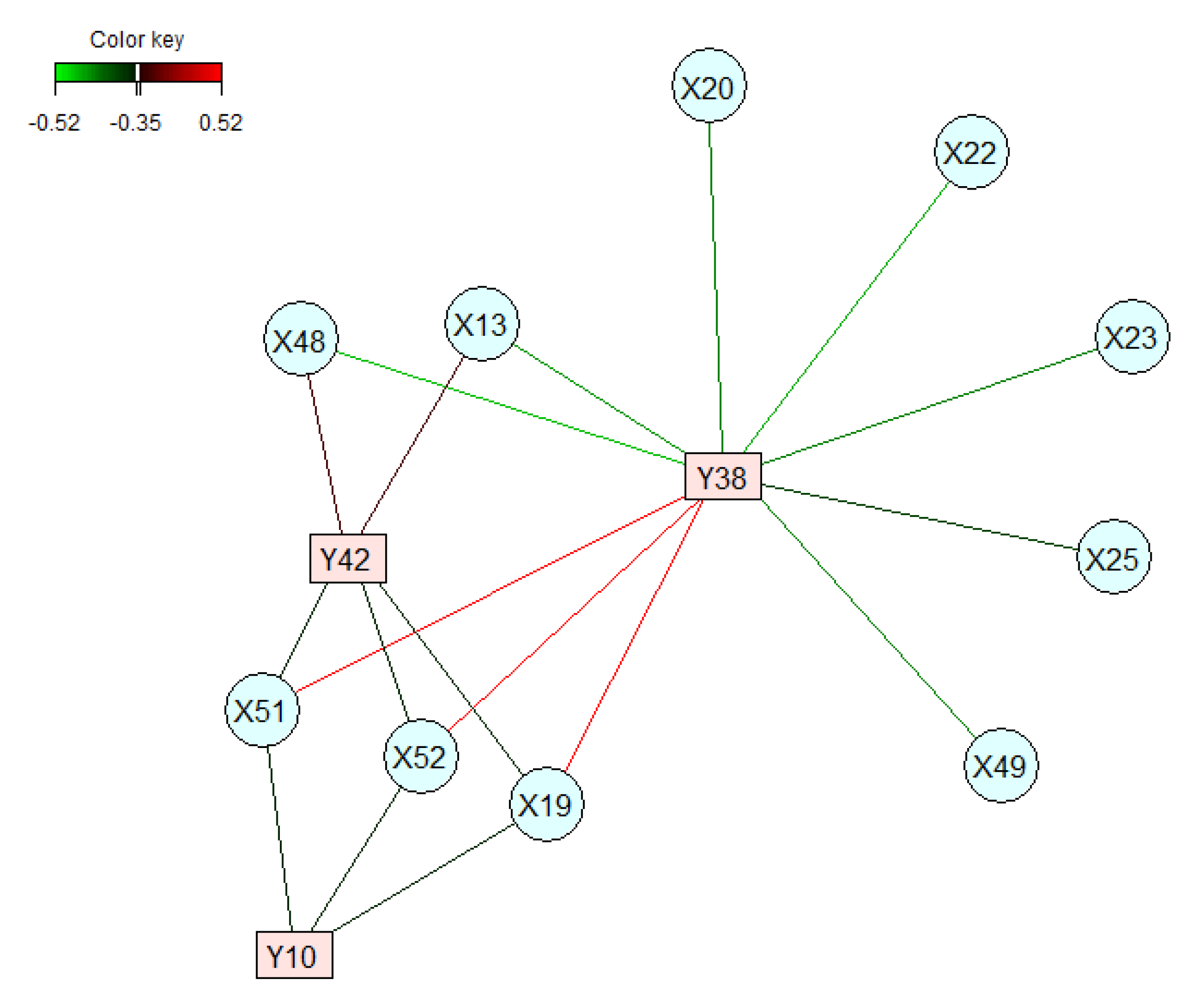
Relevance network is a simple approach for modeling correlation structures between two datasets. This approach generates a graph where nodes represent variables, and edges represent variable correlations. The relevance network, in our study of interest, is displayed through the use of connections between variables of two different types. The relevance networks represent simultaneously positive and negative correlations; the edge colors indicate the nature of the correlation (positive, negative, strong, or weak). It allows the identification of clusters or sub-networks of subsets of variables. Each of these clusters highlight a specific correlation structure between the two types of variables [28].

2.4. Data Collection and Parameters Extraction

The dataset consists in 143 severe or end-staged knee OA patients with clinically and radiographically confirmed knee osteoarthritis. Participants were asked to answer the Oxford Knee Score (OKS) and Pain Catastrophizing Scale (PCS) questionnaires and some measures related to the clinical symptoms during specific tasks and functional tests. For the biomechanical data, participants underwent an in-clinic 3D knee kinematic analysis using the KneeKG${ }^{TM}$ system (Emovi, Canada), which is an objective tool of gait analysis, enabling the biomechanical assessment of the behavior of the knee joint during gait and providing a precise quantitative information [29].

The data collection was approved by Nova Scotia Health Authority Research Ethics Board (Reference number: NSHA ROMEO 1016253), institutional ethics committees of the University of Montreal Hospital Research Center (Reference numbers: CE 10.001-BSP and BD 07.001-BSP), and of the École de technologie supérieure (Reference numbers: H20100301 and H20170901). All subjects provided an informed consent before participation.

2.4.1. Kinematic Data

For each participant, continuous series of 3D knee kinematics of full gait cycles during treadmill walking were collected. 3D kinematics describes the three rotations occurring at the knee joint, flexion/extension (in the sagittal plane), abduction/adduction (Abd/Add) (in the frontal plane), and internal/external rotation (Int/Ext rot) (in the transverse plane). Each gait cycle kinematic pattern was then interpolated to a hundred points (from 1% to 100% of the gait cycle) and averaged to obtain a representative mean gait pattern for each participants and for each rotations. Then, among these 100 measurements for each kinematics curves, a set of 69 parameters routinely assessed in clinical biomechanical studies for knee OA populations has been extracted. These parameters are based on maximum and minimum, varus and valgus thrust, angles at initial contact, and mean values and range of motion (ROM) throughout gait cycles or specific gait subcycles (i.e., loading, stance, swing, etc.). Hereafter, the variables representing these parameters are noted $\mathrm{X}1,\mathrm{X}2,\dots ,\mathrm{X}69$.

2.4.2. Sociodemographic and Clinical Data

Clinical and sociodemographic data regroup 42 measures (

Table 1. Description of the clinical parameters.

$\mathit{Y}$	Variable Description and Range	Mean (SD)
${\mathit{Y}}_{\mathbf{1}}$	Age (years) (40 to 90)	64.75 (8.89)
${\mathit{Y}}_{\mathbf{2}}$	Gender (0:Women; 1:Men)	Women: n = 83; Men: n = 60
${\mathit{Y}}_{\mathbf{3}}$	BMI-Body Mass Index (kg/m2) (21.8 to 58.5)	32.37 (6.05)
${\mathit{Y}}_{\mathbf{4}}$	Measure of health-related quality of life (0.03 to 1)	0.61 (0.22)
${\mathit{Y}}_{\mathbf{5}}$	Visual Analogue Scale for Pain (0 to 95)	44.34 (24.60)
${\mathit{Y}}_{\mathbf{6}}$	Degree of end-stage OA severity (0:Moderate; 1:Severe)	(Moderate: n = 71; severe: n = 72)
${\mathit{Y}}_{\mathbf{7},\dots ,\mathbf{18}}$	Q1, …, Q12 Oxford Question 1 to 12 from Oxford Questionnaire (1 to 5)	1.75 to 3.81 (0.82 to 0.76)
${\mathit{Y}}_{\mathbf{19}}$	Total Oxford Score: Normalized overall Oxford score (15 to 54)	33.15 (9.12)
${\mathit{Y}}_{\mathbf{20},\dots ,\mathbf{32}}$	Q1,..., Q32 PCS: Question 1 to 13 from PCS Questionnaire (0 to 4)	0.61 to 1.38 (1.01 to 1.33)
${\mathit{Y}}_{\mathbf{33}}$	Total PCS score: Normalized overall PCS score (0 to 52)	13.14 (13.22)
${\mathit{Y}}_{\mathbf{34}}$	Rumination score related to depression (0 to 16)	4.43 (4.58)
${\mathit{Y}}_{\mathbf{35}}$	Magnification: Measure of enlargement (0 to 12)	2.98 (3.14)
$X_{\mathbf{36}}$	Helplessness: Measure of Helplessness-related quality of life (0 to 24)	(5.85) (6.11)
${\mathit{Y}}_{\mathbf{37}}$	Index Joint Flex: knee flexion ROM (Range Of Motion) (45 to 154)	123.30 (12.15)
${\mathit{Y}}_{\mathbf{38}}$	Index Joint Ext: knee extension ROM (−29 to 11)	−7.75 (7.02)
${\mathit{Y}}_{\mathbf{39}}$	4 metres Walk (S): Time taken to walk 4 meters, Gait speed in m/s (1.6 to 10.8)	3.40 (1.25)
${\mathit{Y}}_{\mathbf{40}}$	Timed Up and Go (S): The progress of balance, sit to stand, and walking (4.7 to 20.9)	9.21 (3.08)
${\mathit{Y}}_{\mathbf{41}}$	30-s Chair (Reps): Sit-to-stand repetitions (0 to 20)	9.36 (3.73)
${\mathit{Y}}_{\mathbf{42}}$	Frailty Index: Clinical Frailty Scale (CFS) (1 to 6)	2.68 (1.12)

): (1) Sociodemographic characteristics, (2) the degree of end-stage OA severity, (3) the symptoms during specific tasks, and (4) functional tests.

1.

Sociodemographic characteristics ($Y_1$–$Y_5$) such as age and gender.

2.

The degree of end-stage OA severity ($Y_6$) is estimated using Kellgren and Lawrence (KL) scores.

3.

The symptoms during specific tasks are measured using the questionnaires OKS ($Y_7–Y_{19}$) and PCS ($Y_{20}–Y_{33}$). The OKS is a 12-item questionnaire developed specifically for measuring the outcome of total knee replacement (TKR) [30]. It consists of questions covering function and pain associated with the knee. The OKS has demonstrated good validity, reliability, and sensitivity in patients undergoing TKR [31] and thus can be considered a reliable and valid measurement for outpatients with OA. The PCS is a 13-item questionnaire along with three subscale scores assessing rumination, magnification, and helplessness ($Y_{34}–Y_{36}$) developed tohelp quantify an individual’s pain experience, asking about how they feel and what they think about when they are in pain [32].

4.

The functional tests ($Y_{37}–Y_{42}$) simulates the forces encountered during sport-specific activity under controlled clinical conditions.

3. Results and Discussion

Kinematic ($\mathit{X}$ matrix), sociodemographic, and clinical data ($\mathit{Y}$ matrix) were structured in a single database in order to identify the relationships between the two datasets. In this study, the analyses were carried out using mainly the package MixOmics of R.

We evaluated the statistical significance of the RCCA. The p-value for Pillai’s trace statistic is $<0.001$. The first two canonical correlations values corresponding to the first two dimensions are equal to $0.80$ and $0.79$, respectively. These high correlation values show that we can consider a multivariate correlation model and that two dimensions are sufficient to understand the association between the two sets of variables. For the graphical outputs, we empirically adjust a threshold value to $0.35$ such that we can highlight the most important correlations between the two sets of data $\mathit{X}$ and $\mathit{Y}$.

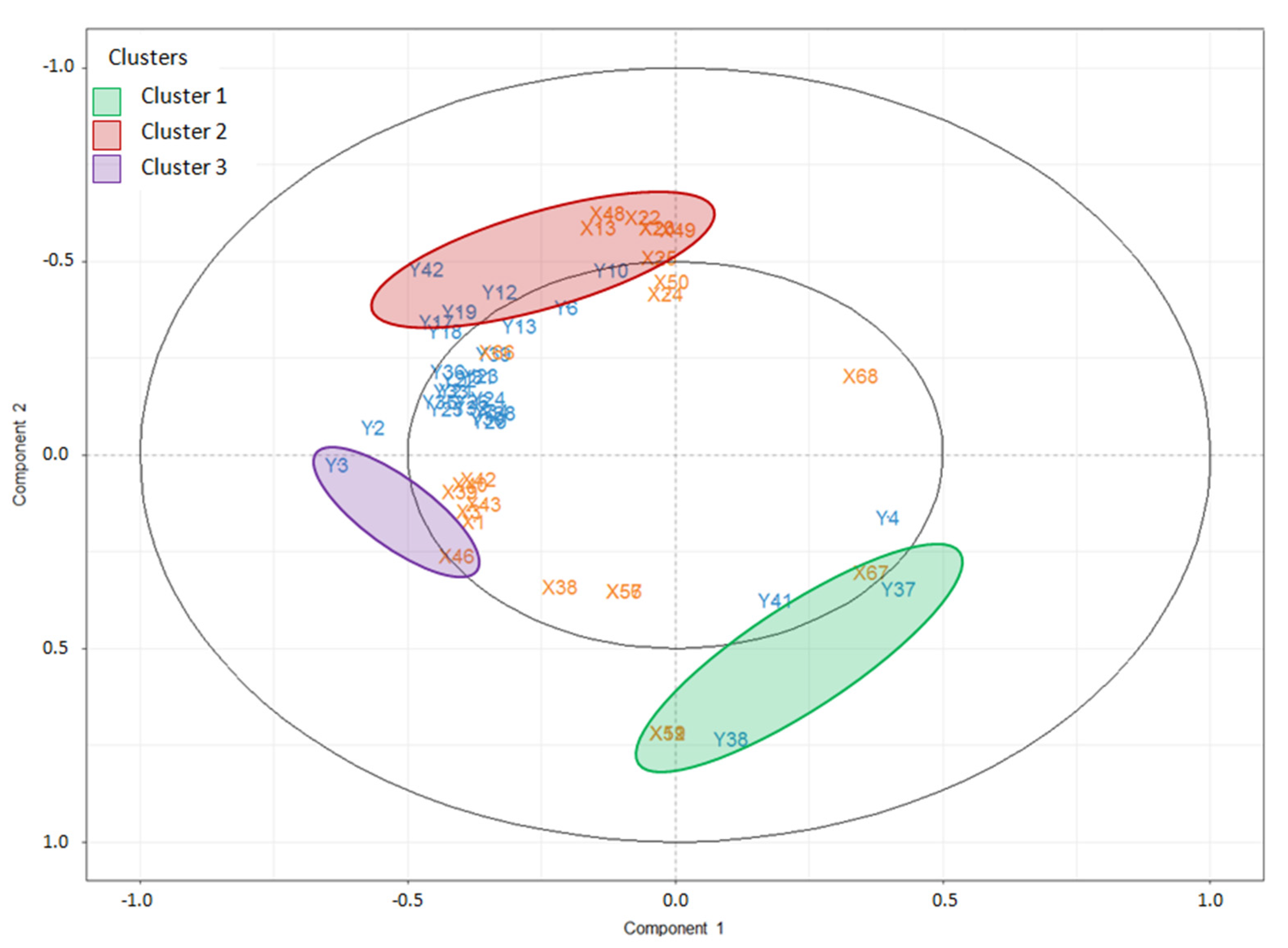
The value of the threshold has been fixed to 0.35 on the basis of the graphical representation of canonical variable correlation (Figure 1). Indeed, most of the variable points are located around the inner-correlation circle with cut-off equal to 0.5. Therefore, we fixed the correlation threshold below this value, i.e., 0.35.

The representation of correlation and cross-correlation variable are displayed in Figure 1, Figure 2 and Figure 3. We distinguish and deduce three clusters (C1, C2, and C3) of highly correlated variables of both sets of data, i.e., each cluster regroups the variables $\mathit{X}$ (kinematic measurements) and the variables $\mathit{Y}$ (clinical parameters). The clusters are visualized in Figure 1, only the variables that are closely located inside the circle of radius between 0.35 and 1 are represented. The clusters C1 and C2 regroup subsets of parameters from $\mathit{X}$ and $\mathit{Y}$ variables. C3 regroups the variables $Y3$ and $X46$ which are highly and positively correlated. The correlation between C1 and C2 is strongly negative. The correlation between C3 and each one of C1 and C2 is negligible because the angle between each pair of clusters (C1, C3) and (C2, C3) is apparently right, so that the correlation is almost null.

CCA, which is a linear subspace analysis, involves the projection of two variable sets $\mathit{X}$ and $\mathit{Y}$ onto a joint subspace such that the correlations between the projected vectors of variables are maximized. The correlation between clusters (between all variables) is quantifying, as explained before, by means of the first two canonical correlations values corresponding to the first two dimensions which are equal to $0.80$ and $0.79$, respectively.

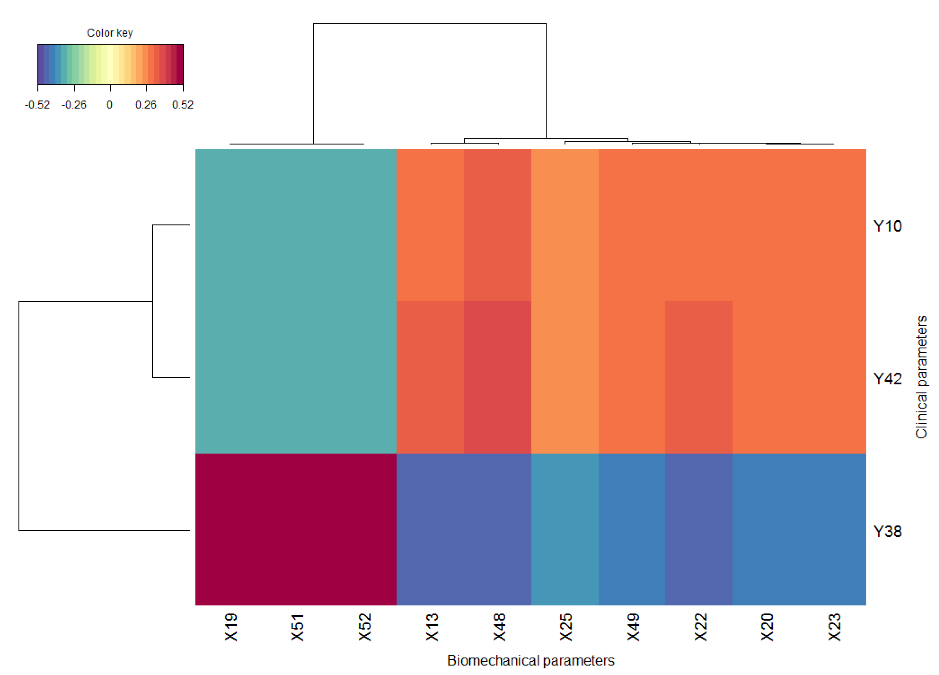
The representation of cross-correlation variable is shown by the heatmap in Figure 2 and relevance network in Figure 3. For the hierarchical clustering in the heatmap, the Euclidean distance was used as proximity measure and the Ward’s method was used for the agglomeration hierarchical clustering procedure [33,34]. The correlation between groups of the variable $\mathit{X}$ and $\mathit{Y}$ is represented by a colored block. The two clusters C1 and C2 identified in Figure 1 are clearly highlighted in Figure 2 by the blue and red blocks that correspond to the two long sections of the dendrograms and are summarized in a single subnetwork in Figure 3, which visualizes simultaneously positive and negative correlations of variables to represent only the strongest cross-correlations.

The representation of canonical variables (Figure 1) and of the cross-correlation variables (Figure 2 and Figure 3) highlights the importance of a combined analysis. For instance, the cluster C3 in Figure 1, which combines the pair of parameters $\left\{Y3,X46\right\}$, is not visualized by the cross-correlation variable representations in Figure 2 and Figure 3 because of the neglected correlation between C3 and the other two clusters C1 and C2. For that reason, the combination of correlation and cross-correlation variable representations implies to consider the cluster 3 with the clusters 1 and 2 as the groups of variables highlighting the highest correlations. From a clinical point of view the cluster C3 is important. As, it emphases the relationship between the BMI and internal/external tibial rotation angle at the end of push-off phase.

Following the combination of these representations, the correlated clinical and kinematic parameters are described in

Table 2. Clusters of correlations between the variables $\mathit{X}$ and $\mathit{Y}$.

Clusters	Variables	Characteristics
C1	X67 X51, X52, X19	Absolute variation in tibial rotation between the end of loading phase and heel strike Flex/Ext total range of motion, absolute value of the Flex/Ext angle, Flex/Ext angle.
	Y38 Y37	Index Joint Ext: knee extension range of motion (ROM) Index Joint Flex: knee flexion ROM
	X13	Flexion angle at heel strike (at initial contact)
	X48	Absolute value of flexion angle at heel strike
	X25	Flexion angle at the end of terminal stance phase
	X49	Absolute value of the minimum Flex/Ext angle during loading phase
	X22	Minimum Flex/Ext angle (Min Flex/Ext) during the gait cycle
C2	X20, X23	Min Flex/Ext during stance phase, Min Flex/Ext during stance and early swing phases
	Y42	Frailty Index: Clinical Frailty Scale (CFS)
	Y10	Q4 OKS: For how long have you been able to walk before pain becomes severe?
	Y12	Q6 OKS: Have you been limping when walking, because of your knee?
	Y17	Q11 OKS: Could you do the household shopping on your own?
	Y19	Total Oxford Score
C3	X46	Internal/external tibial rotation angle at the end of push-off phase
	Y3	BMI

. Cluster C1 regroups kinematic parameter in the sagittal plane related to flexion/extension ROM ($X_{52}$) and transverse plane, which include only the tibial rotation variation value between the end of loading phase and initial contact. Each of these parameters in sagittal and transverse plane are highly and positively correlated with the functional tests indicating the active knee flexion ROM ($Y_{37}$) and flexion contracture ($Y_{38}$) (or extension ROM). The couple of parameters that is important is the one that connects the flexion/extension ROM ($X_{52}$) with the index of joint extension ROM ($Y_{38}$), this corresponds to the red rectangle in the heatmap (2) where correlation are higher than $0.5$.

The second cluster C2 regroups five clinical parameters and seven kinematic parameters. The clinical parameters consist in the functional test of the Clinical Frailty Scale (CFS) index and the Oxford questionnaire (using the scale 1 to 5 of feeling experiencing activities of daily living during the past 4 weeks) that includes four measures Q4, Q6, Q11, and the total Oxford score, which reflects the severity of problems that the patients have with their knee. The kinematic parameters comprise only those of the sagittal plane: flexion angle at initial contact ($X_{13}$ and $X_{48}$) and the end of terminal stance phase ($X_{25}$), and minimum flexion/extension angle during the loading phase, the stance phase, the stance and early swing phases, and during the gait cycle. The functional test of CFS ($Y_{42}$) and the Q4 Oxford Question ($Y_{10}$) have the largest positive correlations with the kinematic parameters in the sagittal plane.

The third cluster C3 relates the internal/external tibial rotation angle at the end of push-off phase and the BMI by a considerable positive correlation (near the inner circle of correlation with a cut-off = $0.5$ in Figure 1).

Finally, the between cluster analysis shows that the correlation between the clinical variables in cluster C1 and the kinematic variables in cluster C2 are strongly negative. The same statement is observed for the correlation between the clinical variables in cluster C2 and the kinematic variables in cluster C1. Moreover, the correlations are negligible between the third cluster C3 and the other two clusters (C1 and C2). As explained above, the angle between each pair of clusters (C1, C3) and (C2, C3) is apparently right, so that the correlation is almost null.

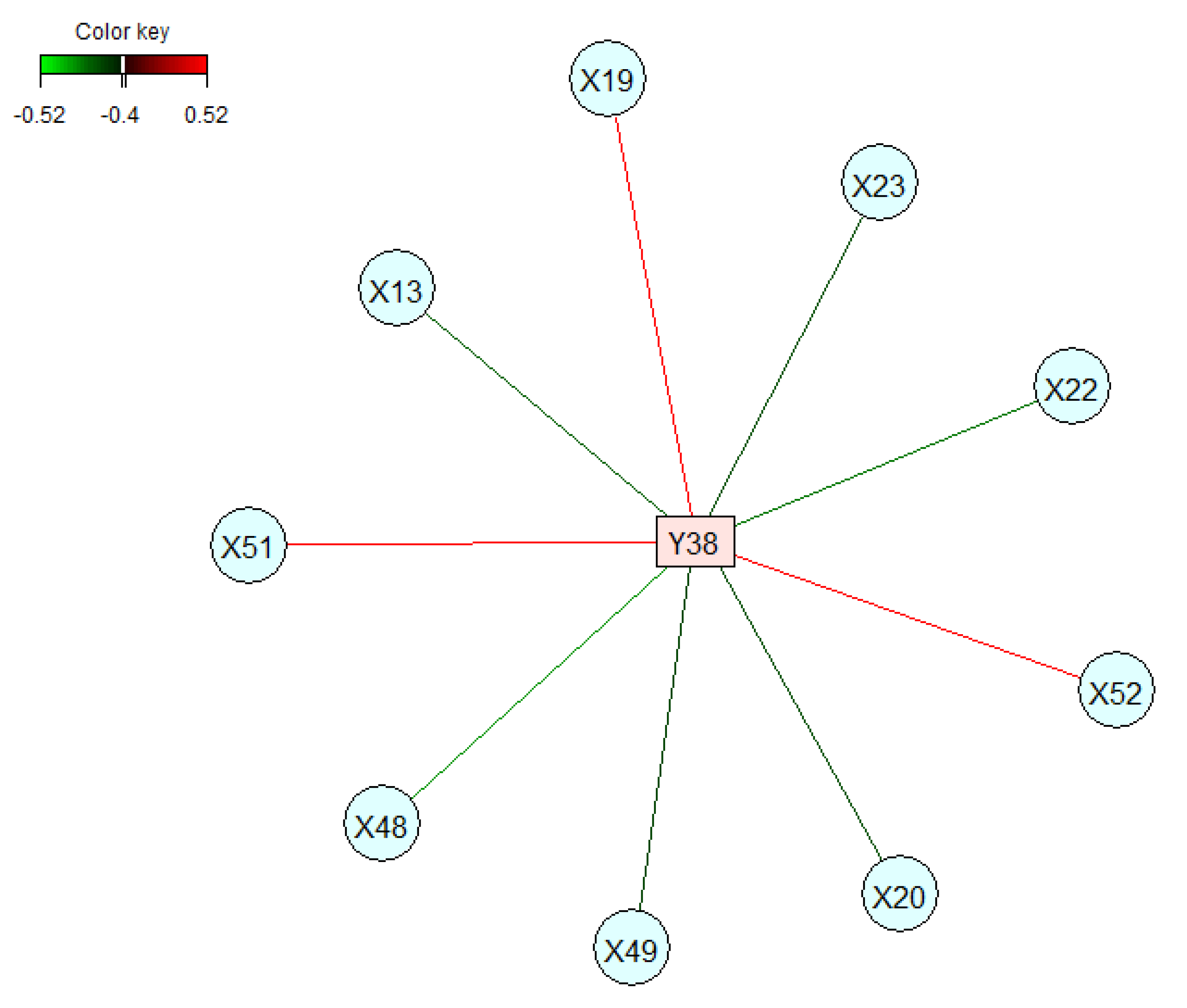
The correlation analysis is expanded to a higher level of threshold. Figure 4 shows a cross-correlation variable representation by relevance networks with a cut-off $=0.40$. We notice that only one subset (of few variables) remains important with higher correlation level. The number of correlated variables is reduced for the most important clinical parameters $Y_{38}$ (in cluster C1) strongly correlated with nine kinematic parameters (in clusters C1 and C2). This analysis shows that increasing the threshold value establishes the most important correlated parameters. However, it leads to the loss of certain correlations that remain significant.

The analysis of correlation between kinematic features of gait waveform data and clinical parameters has been, basically, done using a univariate correlation analysis [9,10,11,12]. The later investigate the relationship between a pair of two variables individually, which could occult important correlation as shown in our previous study [16]. CCA belongs to the family of exploratory analysis and allows investigation of the (simultaneous) relationship between two sets of variables. The multivariate relationship depends on the covariance derived from the two sets of variables which is not the case with the univariate correlation. Moreover, the former is more adapted to investigate the correlation between kinematic and clinical parameters considering the complexity of biomechanical data [15].

4. Conclusions

The purpose of this research was to explore some interesting visual approaches for better analyzing and explaining the multivariate relationships between kinematic measurements and clinical parameters. We performed RCCA and implemented three types of insightful graphical outputs to better understand and interpret the results. The complementarity of these graphical displays was illustrated and allowed us to extract and deduce clusters of sub-sets of variables that are highly correlated, taking into account the positive and negative correlations between variables.

Some parameters of the OKS are clustered with more particular kinematic parameters than others. This was evident by the graphical representation of the data. These associations would not be seen with a regular univariate analysis. The kinematic parameters are in the sagittal plane (according to cluster C2), and it would therefore be possible to consider paying particular attention to these parameters to improve the OKS score. Furthermore, the BMI must be considered if it would act to reduce the rotation deficits in the transverse plane (according to cluster C3).

In conclusion, the visualizations allow a fairly accurate description of the multivariate correlation and aid to identify the clusters underlying higher cross-correlation. Moreover, the combined visualization of the graphical outputs summarizes multivariate data into understandable and meaningful forms for determining the patterns of cross-correlation of the variables relating to the two sets of data. Finally, the method proposed in this study highlights hidden information and allows more understanding of the multivariate correlation.

This study could be expanded using a canonical partial correlation analysis that studies the correlation between two sets of data by controlling another set of confounding variables whose effect will give misleading results if they are not partialled out.