Application of Machine Learning Method to Quantitatively Evaluate the Droplet Size and Deposition Distribution of the UAV Spray Nozzle

Featured Application

Progress in Spray Science and Technology.

Abstract

Unmanned Aerial Vehicle (UAV) spray has been used for efficient and adaptive pesticide applications with its low costs. However, droplet drift is the main problem for UAV spray and will induce pesticide waste and safety concerns. Droplet size and deposition distribution are both highly related to droplet drift and spray effect, which are determined by the nozzle. Therefore, it is necessary to propose an evaluating method for a specific UAV spray nozzles. In this paper, four machine learning methods (REGRESS, least squares support vector machines (LS-SVM), extreme learning machine, and radial basis function neural network (RBFNN)) were applied for quantitatively evaluating one type of UAV spray nozzle (TEEJET XR110015VS), and the case of twin nozzles was investigated. The results showed REGRESS and LS-SVM are good candidates for droplet size evaluation with the coefficient of determination in the calibration set above 0.9 and root means square errors of the prediction set around 2 µm. RBFNN achieved the best performance for the evaluation of deposition distribution and showed its potential for determining the droplet size of overlapping area. Overall, this study proved the accuracy and efficiency of using the machine learning method for UAV spray nozzle evaluation. Additionally, the study demonstrated the feasibility of using machine learning model to predict the droplet size in the overlapping area of twin nozzles.

1. Introduction

Comparing with other pesticide applicators, unmanned aerial vehicles (UAV) can achieve accurate and specific management with its low costs, high efficiency, and mobility [1,2]. UAV crop protection has the characteristics of strong field adaptability and controllable flight parameters, which can be suitable for different crop planting areas [3]. However, UAV spray will produce droplet drift when downwind movement of airborne spray occurs, and a fraction of the dosage does not reach the target area [4,5]. Safety questions and pesticide waste induced by spray drift are the main problems in the UAV spray field [6]. When pesticides drift out of the operation area, it will cause people nearby to have diseases like cancers and allergies [7].

Droplet size is one of the most important characteristic parameters for spray and highly related to spray drift, especially the percentage of fine droplets [4]. The pest control efficiency, on-target deposition, and spray losses are all influenced by droplet size [8]. It is also very important to quantitatively analyze the droplet size distribution for studying the trajectory of the droplet and interaction between droplet and plant target interface [9]. Volume medium diameter (VMD) is one of the most commonly used parameters of the collection of droplets. The volume of all droplets are accumulated from small to large during spraying, VMD corresponds to droplet diameter when the droplet volume equals 50% of the total droplet [10]. Droplet deposition uniformity is also an important aspect of spray characterization [11]. In order to achieve effective diseases and pests control, researchers used many methods to measure the deposition during UAV spraying [12].

The nozzle is the most critical component of pesticide spray technology, which determines the droplet size and deposition distribution [13]. Zhou et al. [14] found that choosing the right nozzle to atomize the droplets with the right size can significantly reduce the drift. Creech et al. [15] found that nozzle type had the most evident effect on the droplet size of the herbicide spray compared with orifice size, herbicide active ingredient, pressure, and carrier volume. Guler et al. [16] studied the droplet deposition uniformity of different nozzles and found the condition of achieving the same spray characteristics of air induction nozzles with a conventional nozzle. Thus, it is of great significance to analyze and evaluate the droplet size and deposition distribution of nozzles.

In recent years, researchers have carried out the analysis and modeling of the nozzle’s droplet size and deposition distribution. Oh et al. [17] developed a three-dimensional Lagrangian model to simulate the deposition patterns produced by twin-nozzle electrospray. Kang et al. [18] established droplet size models for two brands of nozzles, and the two models showed a high degree of confidence after validated by the actual test method. Wang et al. [19] studied the droplets deposition distribution by UAV spraying in the wind tunnel and obtained a prediction model. Hong et al. [20] developed an integrated computational fluid dynamics (CFD) model to predict deposition from air-assisted sprayer onto the tree canopies and demonstrated the ability of this model to evaluate spray application performance.

Machine learning is a branch of artificial intelligence, which can reduce the burden of computing and accelerate the modeling process. It reduces the complexity and improves the performance compared with the physical model [21]. Machine learning methods have been widely used in agriculture, energy engineering, biomedicine, and other fields [22,23,24]. As one kind of machine learning model, artificial neural network model can be well trained and proved to be an alternative numerical simulation technology of CFD under the spray cooling condition [25]. Junior et al. [26] proposed a new approach based on machine learning of the deposition prediction in real time and proved its feasibility. Taghavifar et al. [27] established a prediction model of diesel engine spray characteristics based on artificial neural network and artificial neural network-genetic algorithm; artificial neural network-genetic algorithm showed a better result for modeling.

As far as we know, machine learning methods haven’t been widely investigated in quantitative modeling of the atomization performance of nozzle used for UAV spray. Furthermore, the mean diameter of the multi-nozzle will increase after droplet collision, and the shape of size distribution will also be changed [28]. Thus, the droplet size and deposition distribution in the overlapping area of multi-nozzle spray should be investigated. TEEJET XR 110,015 pressure flat fan-shaped nozzle has been widely used in aerial spray [29,30,31]. In this study, we took TEEJET XR110015VS nozzle as the object and aimed to explore the reliability of using the machine learning method to quantitatively evaluate droplet size and deposition distribution for TEEJET XR110015VS nozzle and twin nozzles condition. The specific objectives were as follows: (1) to establish evaluation model of VMD for TEEJET XR110015VS nozzle using machine learning method; (2) to establish evaluation models of VMD and deposition distribution for twin nozzles condition; (3) explore the feasibility of using machine learning to predict VMD in the overlapping area of twin nozzles by VMD evaluation model of TEEJET XR110015VS nozzle. Overall, this study was the first time to apply machine learning methods to the quantitative evaluation of the droplet size of the UAV spray nozzle, and the reliability of these methods was proved. Additionally, it was also the first time to investigate atomization performance under twin nozzles condition and predict the droplet size in the overlapping area of twin nozzles by using machine learning methods.

2. Materials and Methods

2.1. Spray System

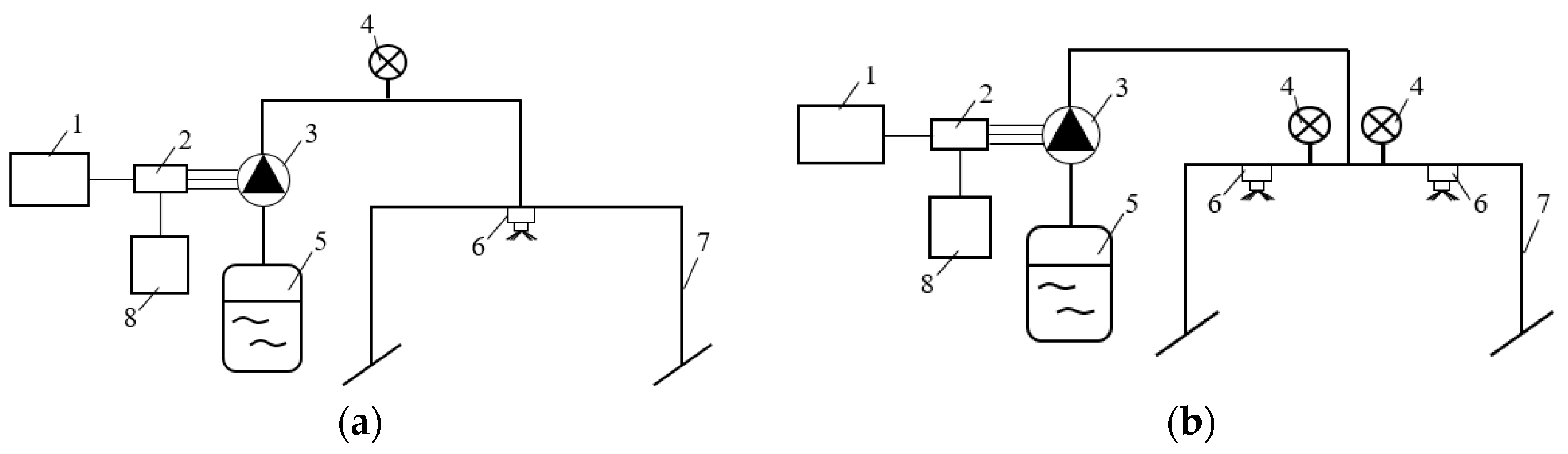
Two spray systems for the experiment were designed as shown in Figure 1.

Two spraying systems consisted of the spray part and the electronic part. The spray part was made up of a three-phase back-flow diaphragm with brushless water pump (Effort tech, Hefei, China, brushless water pump), extended range pressure flat fan-shaped nozzle (TEEJET, USA, XR110015VS), spray tank (10 L), pressure gauge (Chenyi Instrument, Shanghai, China, Shockproof pressure gauge) and support frame. Arduino (Arduino UNO R3), electronic speed control (15 A, 3 S), and battery (12 V, 3 S) formed the electronic part.

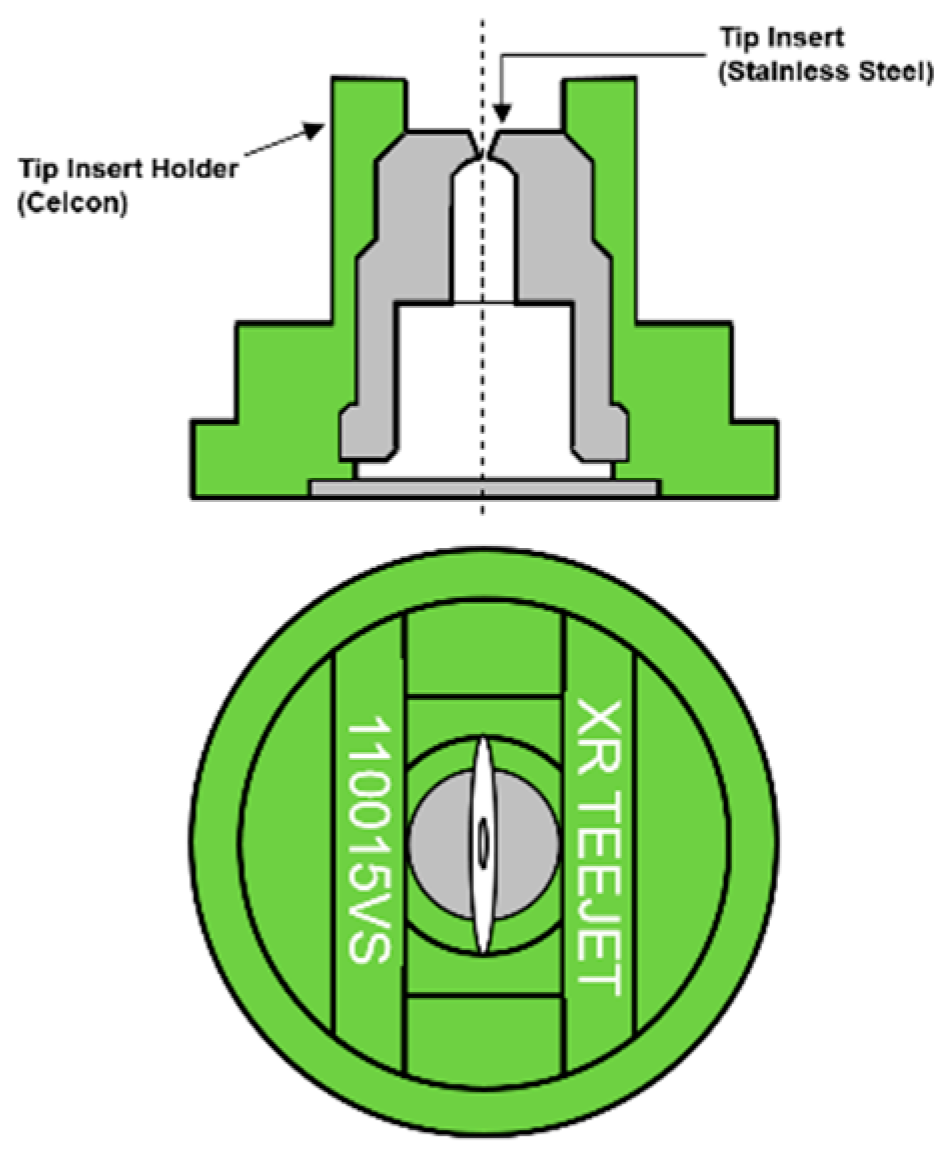
The pressure range of the water pump was 0–0.48 MPa, which can definitely meet the needs of this experiment (0.2 MPa) and easily controlled by the electronic part. The nozzle selected in this experiment (TEEJET XR110015VS) was most commonly used in UAV spraying, it had excellent spray distribution over a wide range of pressures. As shown in Figure 2, The nozzle was mainly composed of the tip insert and tip insert holder. The nozzle could achieve fan-shaped mist spray with a 110° spray angle; it had well spray coverage in high pressure and could be used to reduce the drift in low pressure. A pressure gauge was used to determine that the pressure of spray system was at the set value (0.2 MPa) through experiment. The function of the support frame was to change the spray height of nozzles from 1 m to 2 m and supporting the whole system.

Arduino can provide pulse width modulation (PWM) signal from Pin3 for the experiment with stable and reliable performance when the experiment was operated in two different settings. The Timer2 function of Arduino was used to set the PWM signal and defined the output pin. Electronic speed control could receive the PWM signal from the Arduino and controlled the voltage of the brushless pump, providing 5 V power for Arduino. Battery supplied the required voltage (12 V) needed for these two systems.

2.2. Equipment and Data Collection Methods

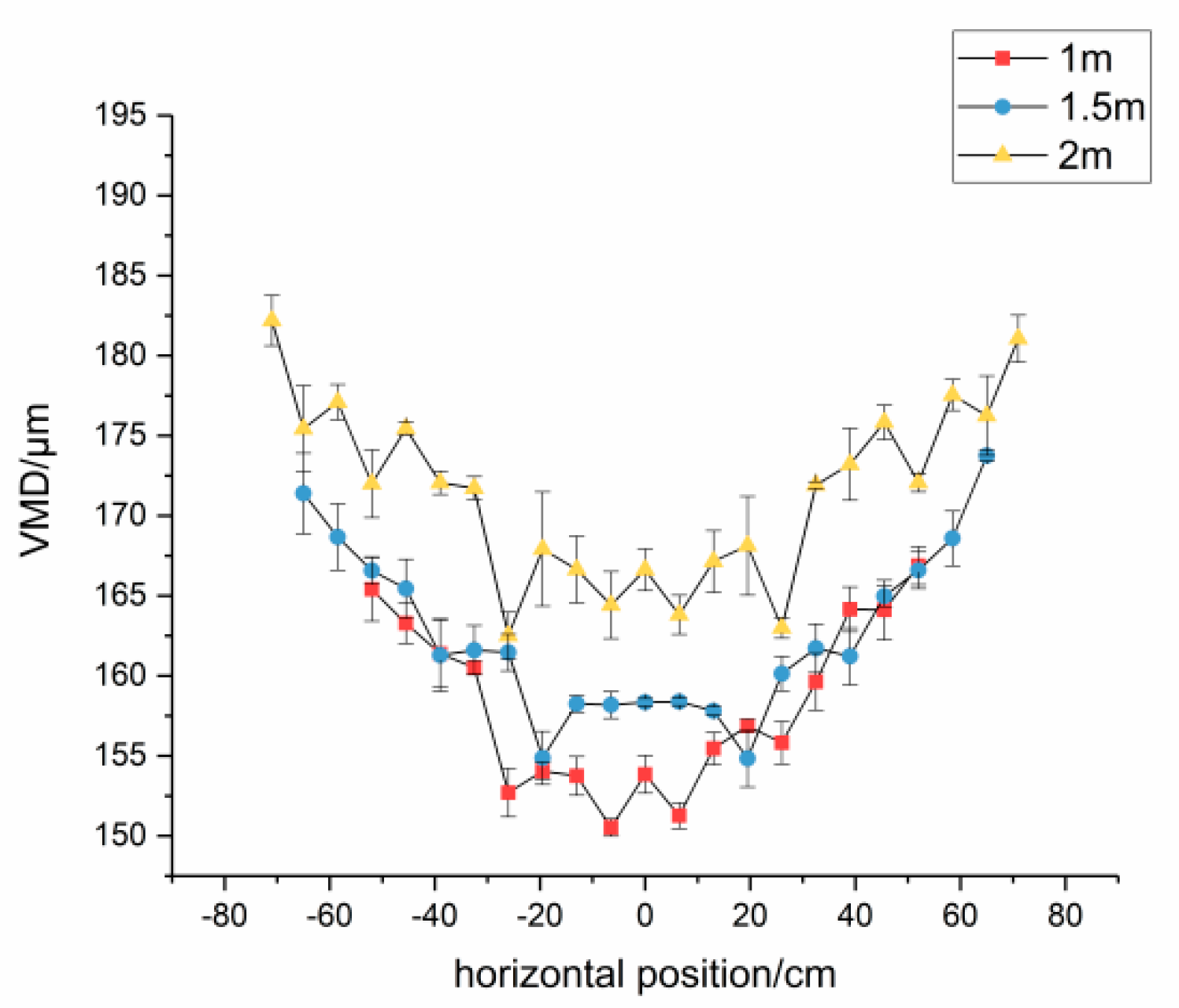
The particle size of the droplets produced by the nozzle and the deposition distribution were two main parameters in this study, the water was used instead of pesticide. The experiment was conducted under the pressure of 0.2 MPa with the environmental temperature at 25 ± 2 °C and the relative humidity of 55 ± 5%. Spray particle size analyzer (NKT Analysis Instrument, Shandong, China, PW180-B) was used to measure the droplet size, the measurement range was 1–1000 µm and the repeatability error was kept within 1%. According to the commonly used UAV spraying flight attitude, spray heights were set to 1 m, 1.5 m, and 2 m.

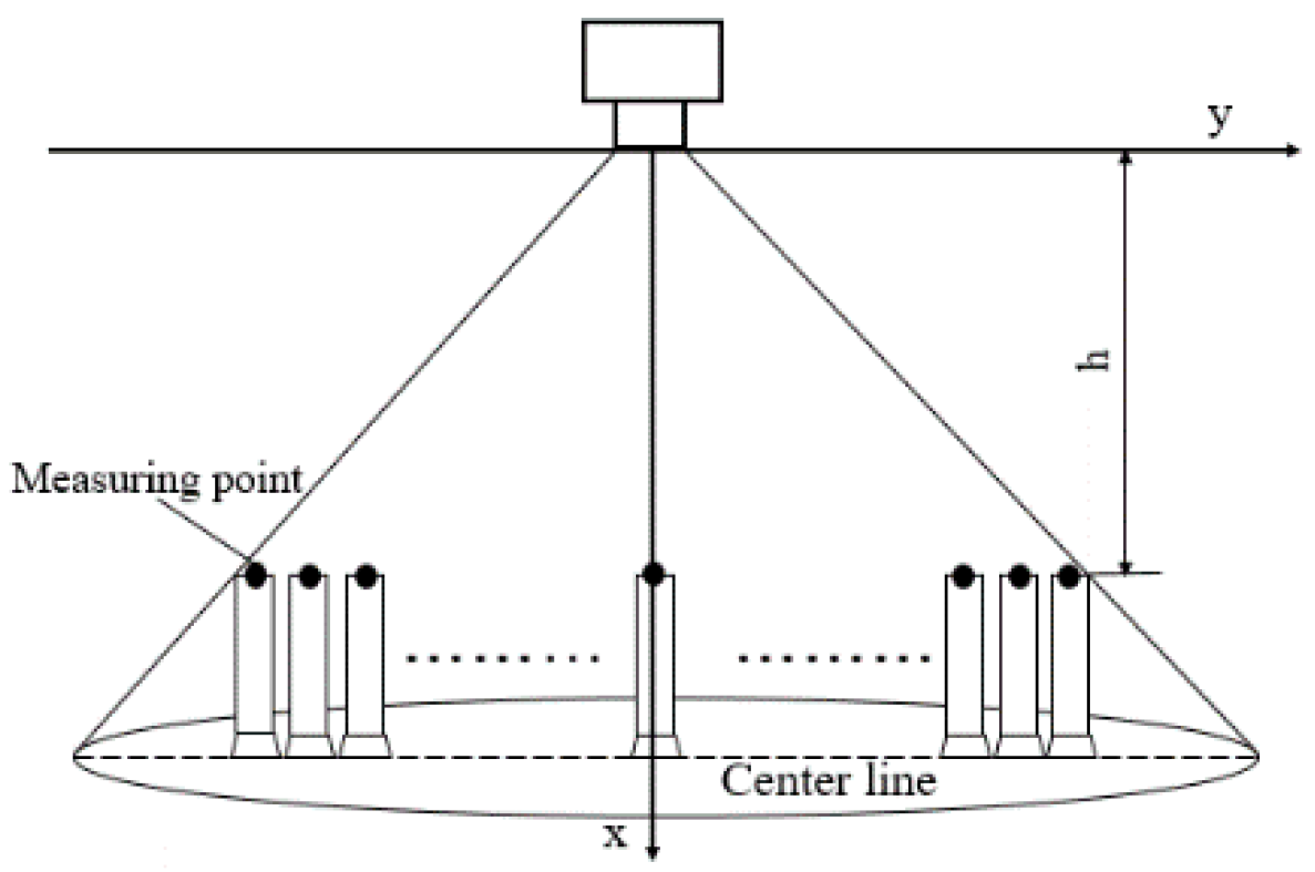
As shown in Figure 3, the deposition was measured by several 100mL measuring cylinders, the center of the upper surface of each measuring cylinder was the position of each measuring point. The experiment put measuring cylinders along the centerline, the time for collecting was 5 min, and the collection repeated for three times. Since the external diameter of the100 mL measuring cylinder was 65 mm (the distance between the centers of two adjacent measuring cylinders is the same as the value of external diameter), we set the distance between each measuring point at the same spray height as 65 mm. the inner diameter of measuring cylinder was 27 mm, and we can get the area of spray for each measuring cylinder, the conversion formula of measured volume and deposition was obtained as follows:

$${\mathsf{\beta }}_{dep}=\frac{V}{0.25\pi d^2}$$

(1)

where ${\mathsf{\beta }}_{dep}$ is the deposition (mL/cm²), V is the measured volume (mL), d is the inner diameter of the measuring cylinder (cm).

The droplet size was measured by passing the laser of particle size analyzer through the measuring point accordingly, and vertically, each experiment collected 60 data of the same measuring point as a group and every test repeated for three times, 60 data were averaged as one measuring value for one measuring point.

The 50% effective deposition determination method was used to determine the spray span of TEEJET XR110015VS nozzle [32]. According to the ASAE standard S341.3, the two-point distance between half of the maximum deposition on both sides was defined as the effective spray span. The deposition was measured in 29 horizontal positions (14 different measuring point on both sizes and one center point) at each height, the measuring cylinders were placed along the center line just as shown in Figure 3, every test was repeated for three times. After this experiment, the spray spans were determined for each height, 1040 mm for 1 m, 1300 mm for 1.5 m, and 1430 mm for 2 m accordingly. The spray span showed symmetry along the spray height direction (axis x).

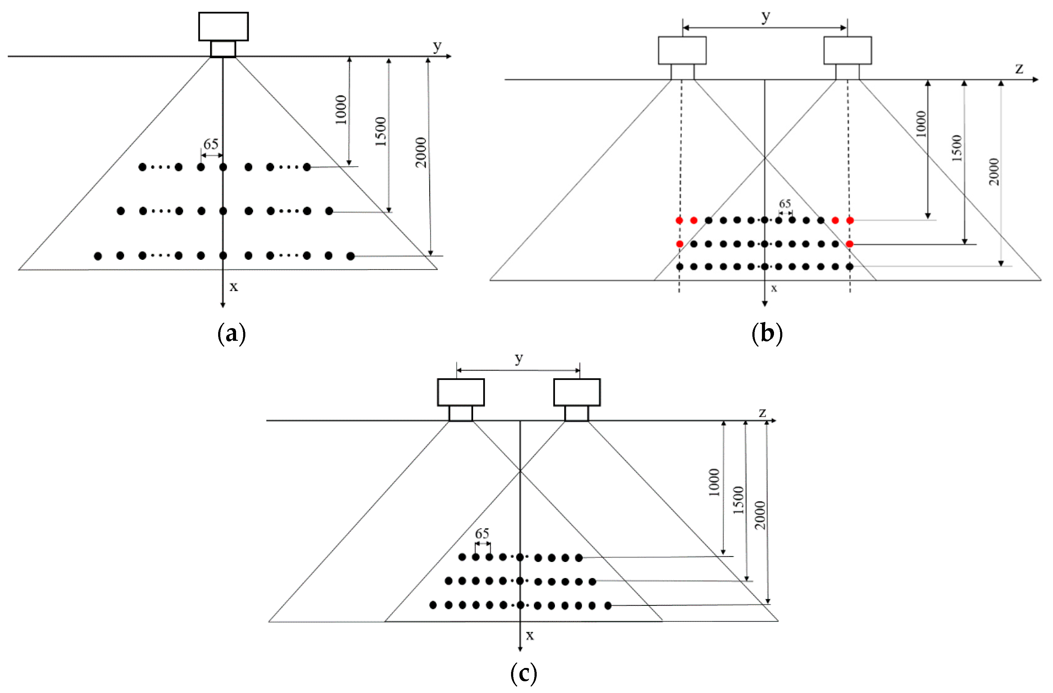
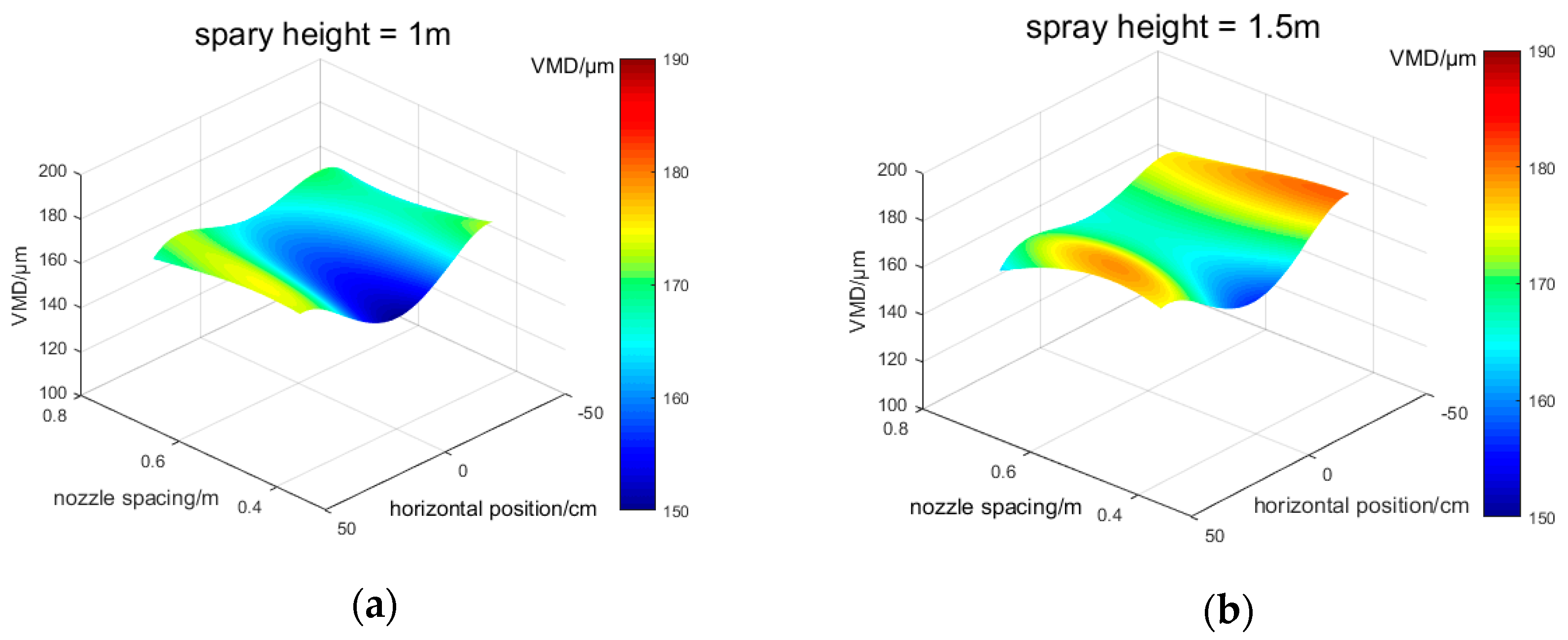
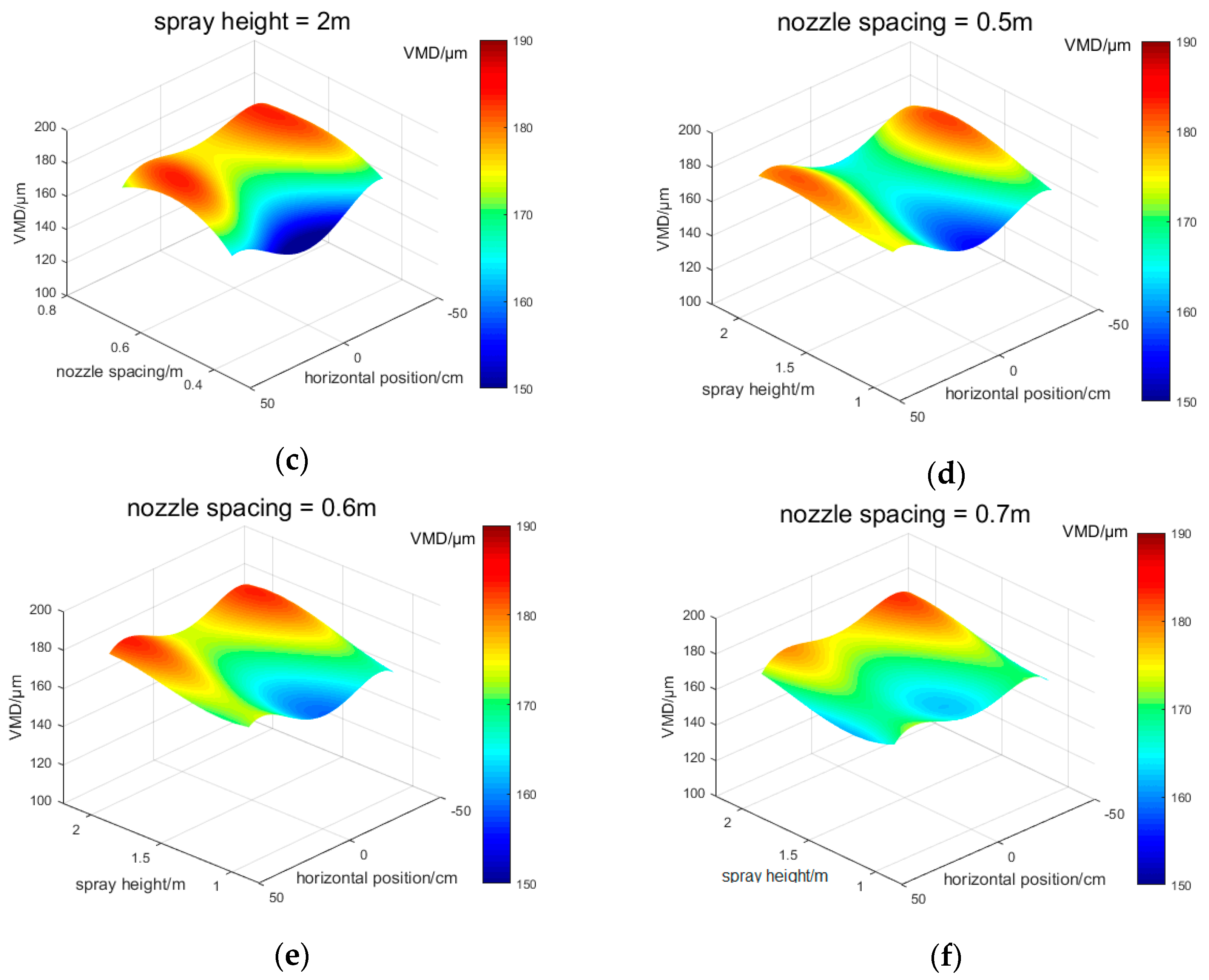
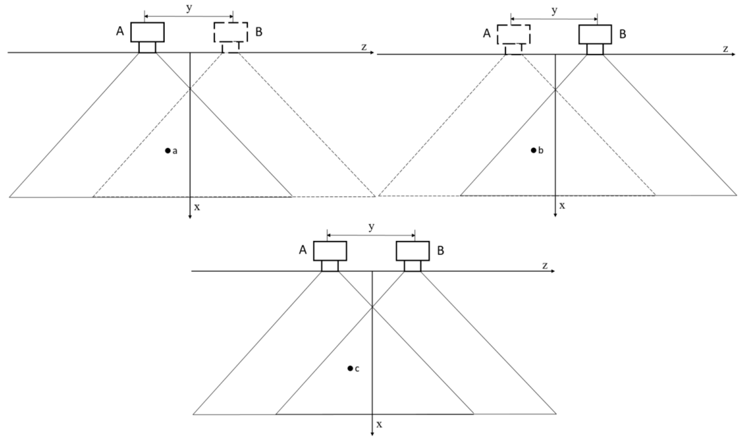
According to preliminary experiment, the spray height remained the sets before (1 m, 1.5 m and 2 m), the measuring points were set along the horizontal line and the interval is 65 mm, the maximum horizontal position were set to ±520 mm, ±650 mm and ±715 mm for each spray height. Additionally, we selected three most commonly used spacing of nozzles in UAV spraying for twin nozzles experiment (0.5 m, 0.6 m, and 0.7 m).

The distribution diagram of measuring points was shown in Figure 4, the VMD values and deposition values obtained from these measuring points were shown in

Table 1. Measured values of volume medium diameter (VMD) and deposition.

	Calibration Set				Prediction Set
Groups	Sum	Range	Mean	S.D.	Sum	Range	Mean	S.D.
A	46	151.26–182.19	165.25	8.13	15	150.53–172.00	163.09	5.64
B	72	154.20–183.00	170.99	7.08	24	156.23–182.30	170.79	7.06
C	72	1.0829–3.2137	1.9144	0.4711	24	1.1818–3.1031	1.8962	0.4609
D	66	154.20–183.82	171.15	7.49	22	156.23–182.74	170.95	7.44

Group A means the group for measured volume medium diameter (VMD) values of the single nozzle (µm); Group B represents all measured volume medium diameter (VMD) values of twin nozzles (µm); Group C represents measured deposition values of twin nozzles (mL/cm²); Group D represents overlapping measured volume medium diameter (VMD) values of twin nozzles (µm). “S.D.” means standard deviation.

. As shown in Figure 4a, the first experiment was to measure the droplet size at each measuring point of the single nozzle, the study took the center of the nozzle as the zero point of the y-axis and collected data of all measuring points within the maximum horizontal position on both sides, group A in Table 1 represents the VMD values obtained by this experiment. In the second experiment (Figure 4b), different position and nozzle spacing were tested in the second experiment, and the VMD values and deposition values were obtained, the zero points of z-axis was at midpoint of the two nozzles, the measuring points were mainly composed of the overlapping area points, points out of the overlapping area and between the vertical lines of two nozzles (red measuring points) were also included, group B and group C in Table 1 represented the VMD values and deposition values obtained by the second experiment. The measuring points of overlapping area were shown in Figure 4c, group D in Table 1 represented the VMD values obtained in this area. Group A, B, C, and D represented the data in Section 3.1, Section 3.2, Section 3.3 and Section 3.4.

Table 2. The mean values, standard deviation, and significant difference for all groups under different experimental conditions.

Groups		Spray Height
	Nozzle Spacing	1 m	1.5 m	2 m
A	\	158.21 ± 5.30 µm c	162.58 ± 5.24 µm b	171.48 ± 5.65 µm a
B	0.5 m	161.15 ± 4.96 µm d	171.33 ± 6.85 µm c	173.12 ± 7.02 µm b
	0.6 m	163.03 ± 4.92 µm d	172.98 ± 3.97 µm b	178.55 ± 2.97 µm a
	0.7 m	167.87 ± 4.00 µm c	168.71 ± 3.96 µm c	178.48 ± 3.99 µm a
C	0.5 m	2.8265 ± 0.2591 mL/cm2 a	1.9069 ± 0.1819 mL/cm2 c	1.6924 ± 0.2573 mL/cm2 d
	0.6 m	2.6962 ± 0.3879 mL/cm2 a	1.8879 ± 0.2492 mL/cm2 d	1.5997 ± 0.2267 mL/cm2 d
	0.7 m	2.1961 ± 0.2630 mL/cm2 b	1.6391 ± 0.1728 mL/cm2 d	1.5222 ± 0.1721 mL/cm2 d
D	0.5 m	161.15 ± 4.96 µm d	171.33 ± 6.85 µm c	172.17 ± 6.40 µm b
	0.6 m	161.72 ± 4.76 µm d	172.98 ± 3.97 µm b	178.56 ± 2.97 µm a
	0.7 m	165.59 ± 3.91 µm d	167.72 ± 3.63 µm c	178.37 ± 3.46 µm a

The data type is mean values ± standard deviation; the same letter note indicates no significant difference at the p = 0.05 significant level, different letters indicate significant differences at p = 0.05 significant level.

shows the result of the mean values, standard deviation, and significant difference for VMD values and deposition values under different spray heights and nozzle spacing. From the saliency analysis, the VMD values in group A showed a significant difference under different spray height. For group B, C and D, the VMD values and deposition values showed significant difference under different nozzle spacing and spray height. On the whole, different experimental conditions in this study can change the droplet size and deposition of the UAV spray nozzle (TEEJET XR110015VS).

2.3. Machine Learning Methods

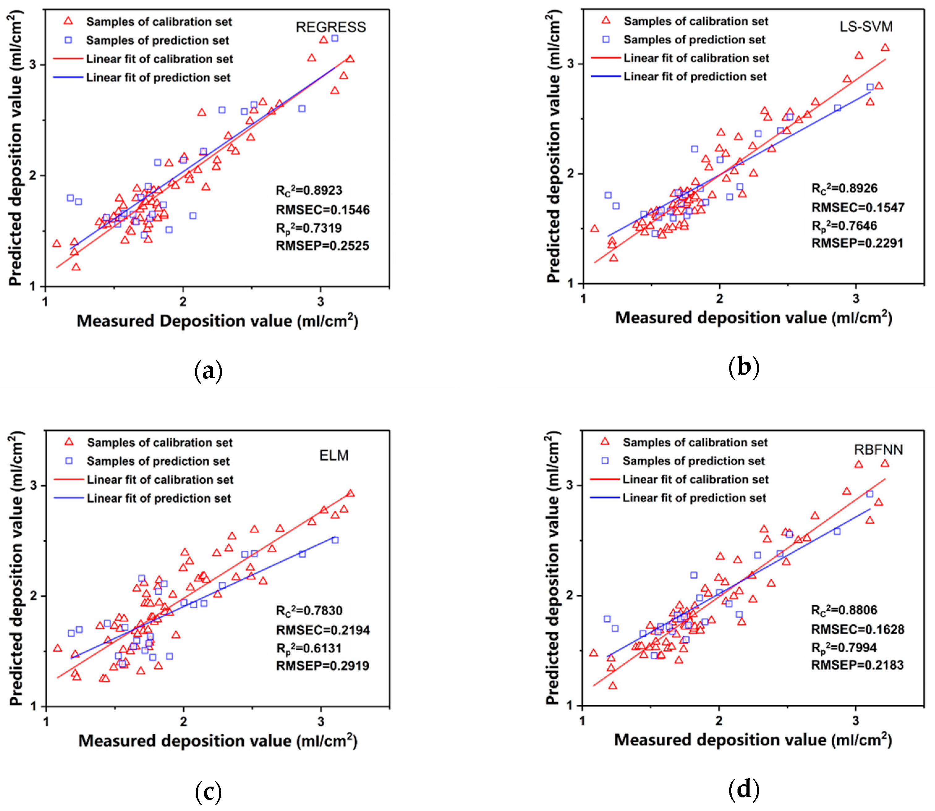
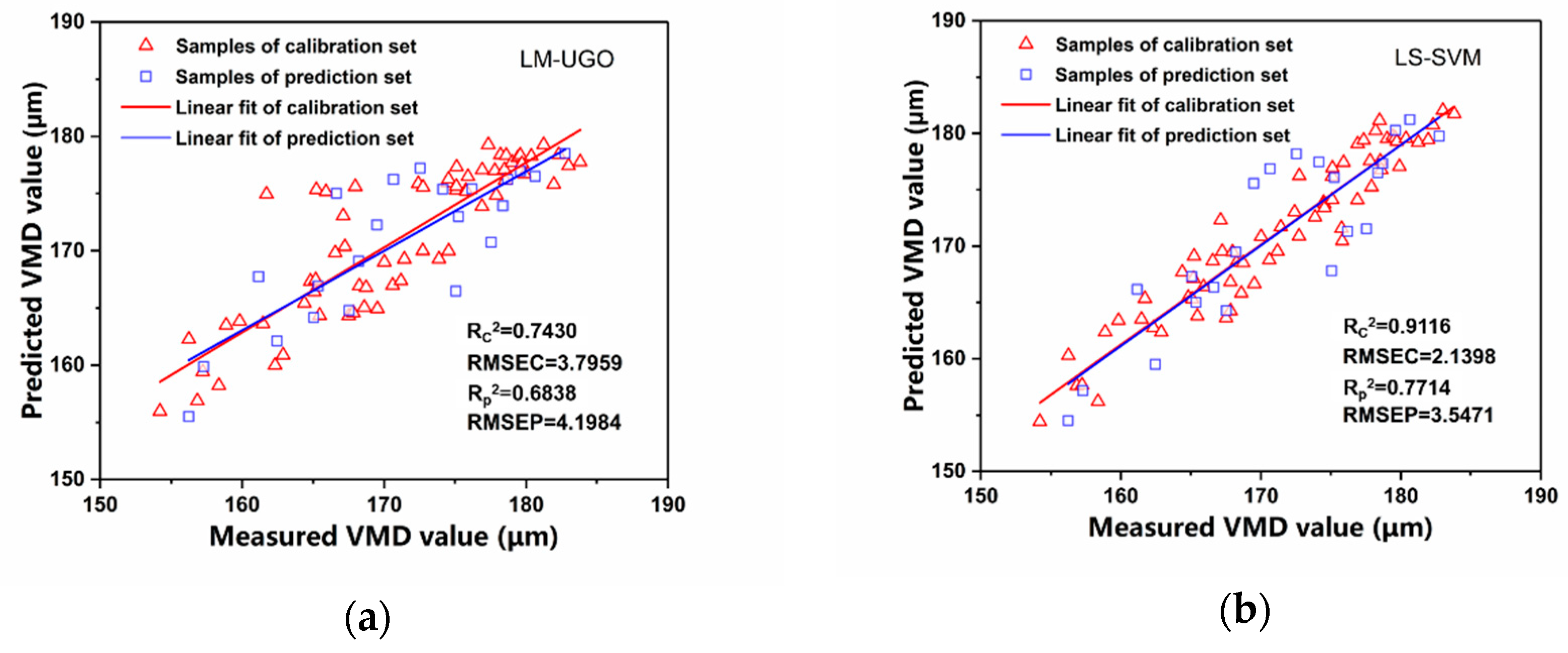
Regress function achieved by MATLAB is an orthogonal least squares method for multiple linear regression; it has been applied in the fields of meteorology, economics [33,34,35]. The least-square algorithm is used in the REGRESS function. Furthermore, REGRESS divides the residuals of observed values of y by an estimate of their standard deviation. The obtained values present t-distributions under a certain degree of freedom. The intervals returned in this function are shifts of the confidence intervals of these t-distributions and centered at the residuals [36]. The F statistic is used to evaluate the significance of the model, the significance level is set to 0.05, and the confidence interval of the coefficient estimation value is set to 95% in this study.

Support vector machine (SVM) is a widely used modeling method, but problems like large workload and long training time occur when this method being used in large size sample. Least squares support vector machines (LS-SVM) can solve these problems with its high efficiency [37]. It is a support vector machine version that involves equality constraints and works with a least-squares cost function [38]. LS-SVM regression used in this study is highly related to regularization networks, Gaussian processes, and reproducing kernel Hilbert spaces, emphasizing the primal-dual interpretations of constrained optimization problems [39]. LS-SVM can solve small-sample, nonlinear, and high-dimensional problems, and the selection of kernel function will affect the final result [40]. Kernel functions are important in SVM with its ability to transform original data from low dimension space to high dimension space. We used the LS-SVM method and chose the radial basis function (RBF) as the kernel function in this study. The penalty coefficient and bandwidth of the RBF (γ) kernel must be determined for better performance.

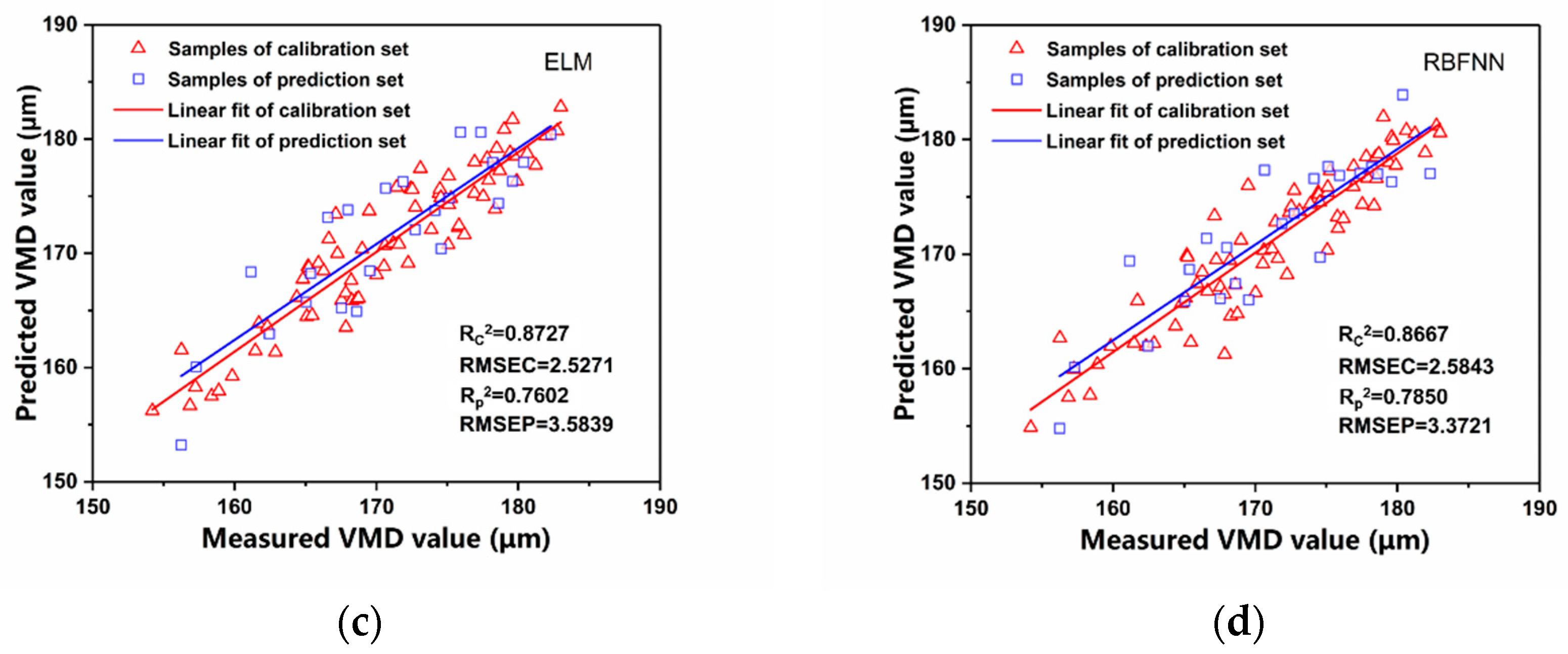
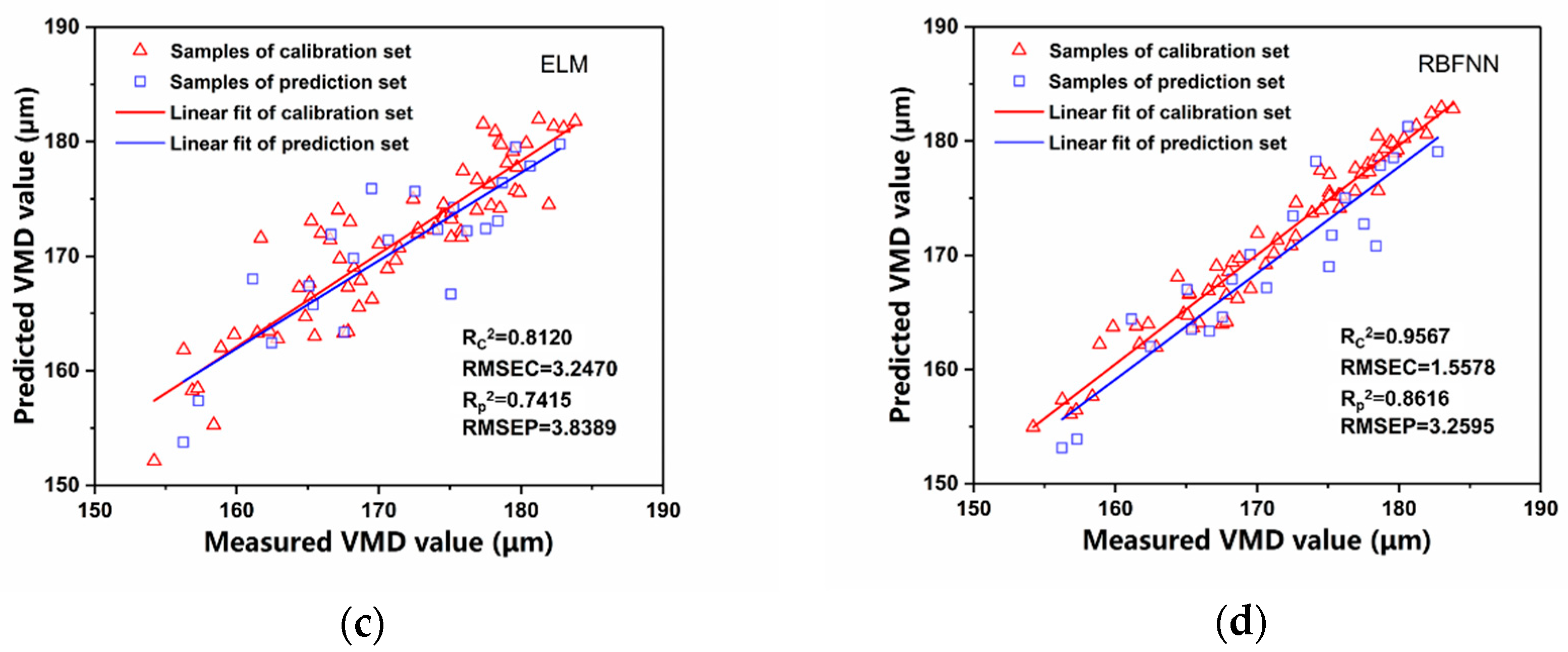
Extreme learning machine (ELM) is a feedforward neural network and has an extremely fast learning speed with a single hidden layer; it can be easily used to many applications by only setting the number of neurons in the hidden layer. It shows the advantage of generalization comparing with most gradient-based learning methods and simpler than neural networks learning algorithms in most cases [41]. ELM was extended from the SLFNs (single-hidden layer feedforward neural networks) with additive or RBF hidden nodes to SLFNs with a wide variety of hidden nodes [42]. It includes an input layer, hidden layer, and output layer, input weights link the input layer to the hidden layer, and output weights link the hidden layer to the output layer. Input weights and hidden biases are randomly chosen, Moore-Penrose generalized inverse is used to determine the output weights [43]. ELM shows faster learning speed than SVM and tends to be more suitable in applications request speed and capability, it also can be applied to nonlinear modeling with its strong nonlinear learning ability.

Radial basis function neural network (RBFNN) is a three-layer feedforward neural network that includes an input layer, a hidden layer and an output layer, taking radial basis function (RBF) as the kernel function. Because of its fast training speed and strong generalization ability, it has been widely used in discrimination and regression analysis [44]. The input layer connected with the external environment and consists of several perception neurons. Due to the output characteristics, there is only one hidden layer in the RBFNN, the hidden layer comprises some hidden nodes. The output layer comprises of some output nodes and acts as a responder for the input layer [45]. RBFNN creates complex decision regions by utilizing overlapping localized regions comprise of simple kernel functions [46]. There are two steps to accomplish the learning procedure of RBFNN, training of the kernel functions centers by using a clustering procedure, and calculating output weights by solving a system of linear equations [47]. The RBF kernels used in this study directly rely on the computation of the relevant distances and reduce the complexity of training. For operating RBFNN on MATLAB, we must determine the best spread coefficient.

2.4. Performance Evaluation

The performance of quantitative models for droplet size and deposition distribution was evaluated by the coefficient of determination (R²), root means square error (RMSE). R² is also called the multiple correlation coefficient and defined as the proportion of variance explained by the regression model. This definition makes it a measure of success of predicting the dependent variable from the independent variables [48]. Rc² and Rp² are coefficients of determination in calibration set and prediction set, respectively, indicating the accuracy of the calibration and prediction models. The error was measured by RMSE, which included root mean square error of validation (RMSEV) and root mean square error of prediction (RMSEP). Smaller RMSE represents a better performance and higher accuracy of the model. The calculation process of these parameters is written below:

$${\mathrm{R}}^2={\left(\frac{{{\displaystyle \sum }}_{i=1}^N\left(\widehat{y_i}-\overline{\widehat{y}}\right)\left(y_i-\overline{y}\right)}{\sqrt{{{\displaystyle \sum }}_{i=1}^N{\left(\widehat{y_i}-\overline{\widehat{y}}\right)}^2{\left(y_i-\overline{y}\right)}^2}}\right)}^2$$

(2)

$$\mathrm{RMSE}=\sqrt{\frac{{{\displaystyle \sum }}_{i=1}^N{\left(y_i-\widehat{y_i}\right)}^2}{N-1}}$$

(3)

where $y_i$ and $\widehat{y_i}$ are the reference and prediction values of measuring point i, $\overline{y}$ and $\overline{\widehat{y}}$ are the average of reference and prediction values, N is the number of measuring points.

3. Results

3.1. Evaluation of Droplet Size for TEEJET XR110015VS Nozzle

The volume medium diameter (VMD) distribution was shown in Figure 5; standard deviations were labeled as error bars; the VMD values of XR110015VS nozzle were increased with the horizontal position and spray height. For the same spray height, when the absolute value of the horizontal position was greater than 26, the tendency of increase for droplet size along the direction became more obvious. The influence of height on droplet size is less than that of horizontal position. This distribution indicated that the proportion of small droplets decreases with the increasing distance of measuring point and nozzle.

According to the Jet theory in the cross-flow environment, the droplet sector spreading with the increase of spray height, more and more small droplets drift away from the spray fan with the velocity of droplet and entrainment air flow attenuates, resulting in the overall increase of VMD. Because of the porous media structure of droplet sector, the entrainment of airflow and the velocity distribution of small droplets, transverse airstream will invade the two flanks of the droplet sector, producing forces on small droplets and blow the droplets off the spray fan, leading to the increase of VMD at the edge of horizontal position.

Quantitative evaluation models based on REGRESS, LS-SVM, ELM, and RBFNN were built to quantify the relationship between spray height, horizontal position, and the droplet size of the nozzle. The number of the calibration set and prediction set was 46 and 15, respectively, with a scale of 3:1. The results of the different models are shown in

Table 3. Results of VMD modeling for TEEJET XR110015VS nozzle.

Model	Parameter [a]	Accuracy of Calibration Set		Accuracy of Prediction Set
		RC2	RMSEC (μm)	RP2	RMSEP(μm)
REGRESS	3	0.9382	2.2011	0.9201	1.9761
LS-SVM	(24.169, 2.445 × 104)	0.9378	2.2026	0.9201	1.8939
ELM	9	0.7413	4.1362	0.6795	3.8519
RBFNN	763	0.9395	1.9960	0.9253	1.9183

Parameters of different models: the highest degree of the polynomial for REGRESS, the bandwidth of kernel function (sig2), and the trade-off between minimum model complexity and minimum training error(gam) for LS-SVM, the number of hidden nodes for ELM, the spreading coefficient for RBFNN.

. Models based on REGRESS, LS-SVM, and RBFNN all had good modeling performance, with Rc² values above 0.92 and RMSEP within 2 µm, indicating these models were capable of predicting VMD values. At the significant level α = 0.05, the F value of 70.2383 was greater than its corresponding critical value, showing the accuracy and robustness of the model based on REGRESS. However, ELM performed bad; the results of the calibration and prediction were worse than the other three models. In the study, we used the model obtained by the REGRESS method to express the VMD distribution. The formula was as follows:

$$\mathrm{z}=147.3650+15.5766x+0.0661y-17.0732x^2-0.0776x·y+0.0073y^2+7.001x^3+0.0222x^2·y-0.0022x·y^2$$

(4)

where x stands for spray height (m), y stands for the horizontal position (cm), and z stands for VMD (μm) (four decimal places are reserved for each coefficient).

3.2. Evaluation of Droplet Size for Twin Nozzles Condition

The REGRESS, LS-SVM, ELM, and RBFNN models were built using spray heights, nozzle spacing, and horizontal positions for quantitatively evaluating the VMD distribution of twin nozzles. The numbers of calibration sets and prediction sets were 72 and 24, respectively with a scale of 3:1.

Table 4. Results of VMD modeling for the twin nozzle condition.

Model	Parameter [a]	Accuracy of Calibration Set		Accuracy of Prediction Set
		RC2	RMSEC (μm)	Rp2	RMSEP(μm)
REGRESS	4	0.9206	1.9949	0.9204	2.0602
LS-SVM	(7.159, 1.490 × 106)	0.9382	1.7634	0.9154	2.2450
ELM	36	0.8727	2.5271	0.7602	3.5839
RBFNN	130	0.8667	2.5843	0.7850	3.3721

Parameters of different models: the highest degree of the polynomial for REGRESS, the bandwidth of kernel function (sig2), and the trade-off between minimum model complexity and minimum training error(gam) for LS-SVM, the number of hidden nodes for ELM, the spreading coefficient for RBFNN.

shows the results of quantitative models based on four different methods. The scatter plot of measured values vs. predicted values of twin nozzles are shown in Figure 6. The result of REGRESS model was almost the same as the LS-SVM model and showed the best performance, with Rc² and Rp² both above 0.9. The F value of 36.8578 was greater than its corresponding critical value, indicating the effectiveness of REGRESS. ELM performed with a Rc² value of 0.8727, and RMSEP of 3.5839 μm, RBFNN with an Rc² value of 0.8667 and RMSEP of 3.3721 μm, both worse than models based on REGRESS and LS-SVM, indicating these two methods were not suitable for VMD prediction. As for the REGRESS model, the study also found that increasing the order of polynomials can improve the Rc² but significantly reduced the accuracy of prediction set; a better result could be obtained by Quartic polynomial regressing with fewer terms and coefficients. LS-SVM had better performance with Rc² and relatively small RMSEP, while quartic polynomial based on the REGRESS model was the best to express the relationship between the independent variable and dependent variable in a simpler way with formula and cured surface graphs.

We used the quantitative evaluation model based on the regress function to express the formula and visualize the VMD distribution of the twin nozzle, the formula was as follows:

$$\begin{array}{l}\mathrm{y}=127.4970-5.6276x_1{}^4+154.6896x_2{}^4-1.0552\times {10}^{-5}{x}_3{}^4-0.1914x_1{x}_2{x}_3\\ \hspace{1em}\hspace{1em}\hspace{1em}+4.1692x_2{x}_3-0.8158x_1{x}_3+57.0344x_1{x}_2-450.9652x_1{x}_2{}^2\\ \hspace{1em}\hspace{1em}\hspace{1em}-0.0019x_1{x}_3{}^2-0.0438x_2{x}_3{}^2+163.9057x_2{x}_1{}^2+0.2832x_3{x}_1{}^2\\ \hspace{1em}\hspace{1em}\hspace{1em}-3.5307x_3{x}_2{}^2-22.5764x_1{}^2+191.8288x_2{}^2+0.0505x_3{}^2-0.4886x_3\end{array}$$

(5)

x₁ stands for spray height (m), x₂ stands for nozzle spacing (m), x₃ stands for horizontal position (cm) and y stands for VMD (μm). (four decimal places are reserved for each coefficient).

As shown in Figure 7, the quantitatively modeling result of VMD for the twin nozzles condition using REGRESS was presented visually. In Figure 7a–c, referring to the relationships between horizontal position, nozzle spacing, and VMD, VMD gradually increased when the measuring point is approaching the bottom of the two nozzles (the edge of two spray fans), presenting symmetrical distribution at the same height. Furthermore, VMD of measuring points near the middle of two nozzles increased evidently with the nozzle spacing. Figure 7d–f showed the relationships between horizontal position, spray height, and VMD. VMD increased with the relative horizontal position and the spray height. The divergence of VMD values along the horizontal direction decreased with the nozzle spacing. These results indicated the difference of droplet size distribution for a single nozzle would cause uneven droplet size distribution after the spray fans were overlapped.

3.3. Evaluation of Deposition Distribution for Twin Nozzles Condition

For quantitatively evaluating the deposition distribution of twin nozzles, the REGRESS, LS-SVM, ELM, and RBFNN models were built using spray heights, nozzle spacing, and horizontal positions. Numbers of the calibration sets and prediction sets were 72 and 24, respectively with a scale of 3:1. The results of the quantitative models are shown in

Table 5. Results of deposition modeling for twin nozzles condition.

Model	Parameter [a]	Accuracy of Calibration Set		Accuracy of Prediction Set
		RC2	RMSEC (mL/cm2)	Rp2	RMSEP (mL/cm2)
REGRESS	3	0.8923	0.1546	0.7319	0.2525
LS-SVM	(2.664, 314.218)	0.8926	0.1547	0.7646	0.2291
ELM	18	0.7830	0.2194	0.6131	0.2919
RBFNN	358	0.8806	0.1628	0.7994	0.2183

Parameters of different models: the highest degree of the polynomial for REGRESS, the bandwidth of kernel function (sig2), and the trade-off between minimum model complexity and minimum training error(gam) for LS-SVM, the number of hidden nodes for ELM, the spreading coefficient for RBFNN.

, and the scatter plot of measured values vs. predicted values of deposition distribution for twin nozzles condition are shown in Figure 8. Performances obtained by LS-SVM and RBFNN methods were both better than models based on REGRESS and ELM, achieving relatively higher accuracy of prediction set. The RMSEP value of RBFNN was smaller than LS-SVM, indicating RBFNN was the best method for deposition distribution quantitative modeling. REGRESS with a Rc² value of 0.8923 and RMSEP of 0.2525 mL/cm² showed the feasibility of the deposition distribution prediction. The overfitting and terms of uncertainty problems also occurred when the order of the polynomial regression based on REGRESS was increasing. ELM models did not achieve expected performance with an Rc² value of 0.7830 and RMSEP of 0.2919 mL/cm² compared with other methods. The results showed that the deposition distribution could be accurately evaluated by nozzle spacing and spatial position of the nozzle using machine learning methods.

3.4. Droplet Size Prediction of Overlapping Area for Twin Nozzles Condition

In order to predict the droplet size of the overlapping area for twin nozzles condition, we established a quantitative model based on different machine learning models. As shown in Figure 9, ‘a’ and ‘b’ represents the VMD value of nozzle A and B for the same measuring point, which were obtained by the REGRESS model of TEEJET XR110015VS nozzle. ‘c’ represents the actual VMD value of twin nozzle measured in the corresponding measuring point of ‘a’ and ‘b’. In order to achieve a better fitting effect of two independent variables and dependent variables with more options, we used Levenberg-Marquardt + Universal Global Optimization (LM-UGO) instead of REGRESS. Software package 1stOpt was used to realize LM-OGO. Quantitative models based on LM-UGO, LS-SVM, ELM, and RBFNN were built to quantify the relationship between ‘a’, ‘b’ and ‘c’. The numbers of the calibration set and prediction set were 66 and 22, respectively with a scale of 3:1.

Table 6. Results of VMD modeling for the overlapping areas of the twin nozzles condition.

Model	Parameter [a]	Accuracy of Calibration Set		Accuracy of Prediction Set
		RC2	RMSEC (μm)	Rp2	RMSEP(μm)
LM-UGO	/	0.7430	3.7959	0.6838	4.1984
LS-SVM	(0.599, 22.789)	0.9116	2.1398	0.7714	3.5471
ELM	36	0.8120	3.2470	0.7415	3.8389
RBFNN	35	0.9567	1.5578	0.8616	3.2595

Parameters of different models: the bandwidth of kernel function (sig2), and the trade-off between minimum model complexity and minimum training error(gam) for LS-SVM, the number of hidden nodes for ELM, the spreading coefficient for RBFNN.

shows the results of four models. The scatter plot of measured values vs. Predicted values of twin nozzle VMD are shown in Figure 10. For VMD, the prediction of overlapping area, RBFNN achieved the best performance with an Rc² value of 0.9567 and RMSEP of 3.2595 μm, indicating the good potential of this machine learning method. The results obtained by LS-SVM and ELM methods showed expected performance, LS-SVM with an Rc² value of 0.9116, RMSEP of 3.5471 μm, and ELM with an Rc² value of 0.8120, RMSEP of 3.8389 μm. The large RMSE values and the scatter points deviated from the fitting line indicated the LM-UGO was not a good candidate for quantitative modeling of VMD relationship. The results indicated that the regression model of a single nozzle could be used to predict the droplet size of the overlapping area for twin nozzles condition.

4. Conclusions

In this study, machine learning methods were applied to accomplish droplet size and deposition distribution quantitative evaluation for TEEJET XR110015VS nozzle. REGRESS and LS-SVM achieved good performance for droplet size quantitative evaluating of single and twin nozzles, with Rc² and Rp² values both above 0.9. The droplet size distribution of twin nozzles was visualized by formula obtained from REGRESS, the principles leading to the droplet size distribution of single and twin nozzles were also explained. Additionally, RBFNN showed great effectiveness for deposition distribution quantitative evaluation for twin nozzles condition with the best Rp² value of 0.7994 and RMSEP value of 0.2183 mL/cm². The results of Models for deposition distribution were inferior to models for droplet size distribution but still promising. Finally, the model of a single nozzle based on REGRESS was used to predict the droplet size in the overlapping area of twin nozzles; RBFNN showed the best performance for quantitatively predicting, with an Rc² value of 0.9567 and RMSEP of 3.2595 μm.

This study provided a novel and precise method for effective quantitative evaluation of droplet size and deposition distribution for UAV spray nozzle. The quantitative determination of droplet size distribution for UAV spray nozzle can help to control the spray drift and provide a basis for realizing uniform deposition and efficacy of UAV spraying. Furthermore, the study showed the feasibility to predict droplet size of the overlapping area by using the model based on machine learning methods, providing a basis for studying the droplet size distribution of a multi-nozzle spray. In future studies, more types of UAV spray nozzles and more measuring points will be studied under different conditions, the effect of the wind field and the interaction between droplets and crop leaves also need to be investigated in the future experimental design.