Article

Experiments and Modeling for Investigation of Oily Sludge Biodegradation in a Wastewater Pond Environment

1
Department of Chemical and Natural Gas Engineering, Texas A&M University-Kingsville, Kingsville, TX 78363, USA
2
Chemical Engineering Department, Al-Imam Muhammad Bin Saud University, Riyadh 11432, Saudi Arabia
3
Techevon LLC, Lancaster, SC 29720, USA
4
Aker BP, 4020 Stavanger, Norway
5
Arcanum Infrastructure, Raven Butene-1 LLC, Baytown, TX 77521, USA
*
Author to whom correspondence should be addressed.
Appl. Sci. 2020, 10(5), 1659; https://doi.org/10.3390/app10051659
Submission received: 21 December 2019 / Revised: 18 February 2020 / Accepted: 24 February 2020 / Published: 1 March 2020
(This article belongs to the Special Issue Hazardous Waste Treatment)

Abstract

:

Potential Application

Remediation of oily sludge ponds at historic refinery sites and related petroleum facilities.

Abstract

Historic operating and abandoned refineries frequently contain ponds or lagoons that contain oily sludge from historic wastewater treatment processes and separator sludge disposal activities that occurred prior to the implementation of regulations forbidding such disposal. These oily sludge-containing wastewater ponds represent a long-term liability at older operating refineries or abandoned refinery sites. Dewatering and solidification/stabilization are the most common technologies used to treat these sludges; however, these approaches are labor, equipment, and material-intensive. For sites where the time required to complete treatment is not a high priority, biodegradation treatment may be effective for final site remedy. The objective of this study was to investigate potential improvements in oily material biodegradation using dispersants and petroleum-degrading microbial consortia, along with the modeling of this system. The oil dispersed with mixing or remaining in the bulk aqueous phase with biodegradation was measured using methods from a dispersant effectiveness test. The experimental results indicated that mixing at levels of 200 rpm or higher resulted in positive effects on both the extent of hydrocarbon dispersion (80 to 90% of oil dispersed) and the biodegradation of the oil phase (50 to nearly 100% degraded), while the modeling results, taken along with the experimental results, indicated smaller dispersed phase droplet sizes and promoted more efficient biodegradation.

1. Introduction

Many older operating refineries or abandoned refinery properties have oily sludge ponds that require remediation. Dewatering, solidification/stabilization, incineration, or oxidation are the most common technologies used to treat these sludges; however, these approaches are labor, equipment, and material-intensive [1,2]. Frequently, cleanup of such sites may be drawn out, due to either a financially insolvent responsible party, or the site at present being within an existing operating facility, and thus RCRA (Resource Conservation and Recovery Act) closure may not be immediately required. In these instances, a method of treatment/degradation such as aerobic biodegradation, which can be slow but still effective under the proper conditions [2], may represent a desirable alternative to both the owner/responsible party and the regulatory agency. A primary challenge in applying biodegradation to oily sludge material is the significantly lower aqueous availability and biodegradation rate of the heavier hydrocarbons, including polynuclear aromatic hydrocarbons (PAHs) [2].
This research considers the use of oil dispersants and microbial consortia developed for open ocean crude oil spill treatment applied to this particular problem of oily sludge treatment via aerobic biodegradation. This treatment would occur in a more controlled and potentially engineered environment as compared to the open ocean, such as a pond or large basin. The use of surfactants or dispersant formulations, along with the addition of petroleum-degrading microbial consortia, for treatment of non-aqueous phase liquids (NAPL) such as oily sludges has been considered by others [1,2,3]. Rahsepar et al. [4] applied the dispersant Corexit in testing the biodegradation of a non-weathered and a weathered crude oil and determined that the active control in which the dispersant was not included indicated a greater extent of biodegradation, as compared to the test conditions that included the dispersant. Overholt et al. [5] found that the addition of the dispersant Corexit hindered the biodegradation of crude oil by the species Acinetobacter, while oil biodegradation by the species Alcanivorax was improved with the addition of Corexit. Pan et al. [6] conducted experiments on oil dispersion at different mixing speeds (correlated to energy dissipation rates) and different mixing durations, and found that oil dispersion improved slightly with an increase in the mixing time. These cited works primarily relate to the open ocean crude oil spill management problem, rather than an engineered oily sludge biodegradation challenge. The work reported herein is an initial effort to assess dispersing and biodegradation of an oil sludge surrogate (crude oil) in a controlled laboratory setting using dispersants and microbial consortia developed and utilized in oil spill management, with the end objective being the selection of techniques for scale-up to a pond-based engineered treatment system. Other works similar to this, utilizing oil spill dispersants and microbial consortia for the purpose of oily sludge biodegradation in a controlled environment, have not been recognized by these authors. The specific objective of the research presented herein is to measure the dispersant effectiveness and biodegradation extent of the oil sludge surrogate in several laboratory-controlled environments with varying mixing intensity and scale beyond the typical small flask scale used in the literature cited above. The modeling of oil dissolution from droplets and aqueous phase biodegradation was also included as an objective.
Preliminary results indicate the effectiveness in dispersing NAPL is primarily dependent on mixing intensity, and secondly on the dispersant used. The dispersant effectiveness is correlated with energy dissipation of mixing, and greater effectiveness is demonstrated with different types of impellers. Also, the mean dispersed oil drop diameter is calculated based on energy dissipation value. The biodegradation extent, as measured by residual oil content in the aqueous phase, is hampered by some dispersants and not others, and also exhibits a moderate dependence on the mixing intensity.

2. Materials and Methods

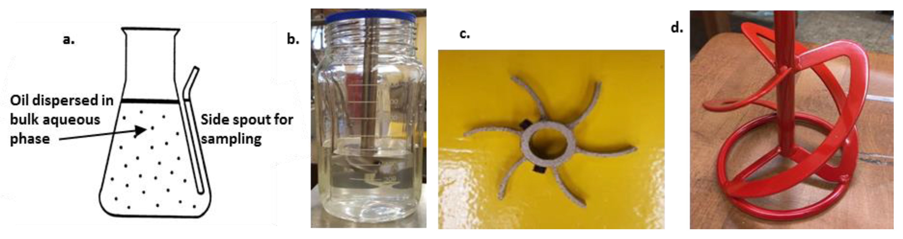
2.1. Experimental Methods

The dispersant effectiveness (DE) test was implemented using the USEPA protocol developed for the assessment of dispersant formulations for oil spill cleanup/treatment [7]. This DE procedure was implemented with dichloromethane (DCM) as the extraction solvent and concentration of residual oil determined by spectrophotometric absorbance of extracted oil, measured at wavelengths of 340, 370, and 400 nanometers, as specified in the protocol. The DE is determined by direct measurement of the concentration of oil dispersed in the continuous phase after dispersant addition and completion of the mixing protocol, as determined using absorbance versus concentration calibration curves established for each oil and dispersant mixture, and for each of the three spectrophotometer wavelengths. The oil concentrations calculated based upon each separate wavelength measurement are averaged to give the final estimated dispersed oil concentration in the continuous phase. This test was extended to different size containers and different means of mixing (orbital shaking of flask, stirring with paddle mixer or helical ribbon mixer (see Figure 1)) to evaluate the dispersion of oil by different means and at different scales (250-mL Erlenmeyer flask, 1000-mL baffled jar flask, or a 30-L plastic container with no baffles). The amount of oil added and the ratio of oil to dispersant were also altered in this work. In particular, one set of experiments for dispersant effectiveness was conducted using a fraction factorial design (see Table S1 in the Supplementary Materials), with mixing speed, dispersed phase volume, dispersant type, and dispersant to oil ratio as the independent variables. Aside from the paddle mixer, the helical ribbon mixer was selected for testing because this type of impeller is used in commercial wastewater pond mixing equipment (Solarbee and Gridbee, Medora Corporation, Dickinson, ND, USA). The oily material used for testing in the entirety of this work was West Texas Crude Oil (WTCO), sold as West Texas blend from ONTA Corp. The dispersants tested included a confidential dispersant (commercially available product), Petroclean (Alabaster Corporation, Pasadena, TX, USA) and FFT (FFT Technologies, Charleston, SC, USA).
The calculation of the oil droplet average size was based upon oil fluid properties and the energy dissipation. Equation (1) below is based on the Weber number theory to predict the average equilibrium droplet size (Equation (1)), as presented by Pan et al. [6]. This method is based on a semi-empirical theory, the Sauter mean droplet diameter, D32, at equilibrium, as previously developed by Hinze [8], Calabrese et al. [9], Chen and Middleman [10], and Shinnar and Church [11].
D 32 D = A ( ρ c ( ε D ) 2 3 D / σ ) 3 / 5 [ 1 + B ( ρ c ρ d ) 1 2 μ d ε 1 3 D 32 1 3 / σ ] 3 / 5
In Equation (1), D is the diameter of the vessel (m), σ is the oil-water interfacial tension (N/m), ε is the average energy dissipation rate (W/kg), ρd is the density of the dispersed phase (kg/m3), ρc is the density of continuous phase (kg/m3), μd is the viscosity of the dispersed phase (N/m), and A and B are system-dependent constants based on geometry and impeller. Wang et al. found that the constants A and B for μd < 500 cP are 0.054 and 4.08, respectively [12]. The fluid properties used in this instance to calculate the droplet size are listed in Table 1.
The energy dissipation and applied energy were calculated utilizing Equations (2) and (3), based upon the rotational speed and impeller diameter.
P = N p · ρ c · N 3 · d 5
ε = P V
where P = power applied (watts), Np = power number, 𝜌c = density of water (kg/m3), N = impeller rotational speed (rpm), d = diameter of the impeller (m), and V = mass of the continuous phase (kg). Depending upon the type of impeller and the presence or absence of baffles, the appropriate power number correlations were used and calculated. Specifically, for the unbaffled container and paddle impeller, the power number was calculated using the unbaffled condition equations of Kamai et al. [13,14], while for the baffled flask and paddle impeller, the baffled equations presented by Kamai et al. were used. For the unbaffled container and the helical ribbon impeller, the power number was calculated using the helical ribbon equations given in the reference of Furukawa et al. [15]. The amount of power actually applied was not measured in these experiments, but only estimated by the calculation of the power number and use of Equation (2).
Biodegradation testing was conducted using the addition of an oil and dispersant NAPL phase, mixing to disperse the NAPL in the same or similar manner as for the dispersant effectiveness test, then inoculating with Oppenheimer formula, which consists of microbial strains of Actinobacteria, Gammaproteobacteria, Bacteroidia, Flavobacteriia and Bacilli (Oppenheimer Biotechnology, Austin, TX, USA, relative amounts of the different bacterial species not provided nor measured), and subsequently incubating with passive aeration and mixing via orbital shaking at room temperature. The M9 minimal salts medium used as the nutrient broth for the biodegradation testing consisted of (per liter of distilled water) 6.0 g/L potassium phosphate (KH2PO4), 3.0 g/L ammonium chloride (NH4Cl), 9.0 g/L sodium phosphate dibasic (Na2HPO4), 2.1 g/L potassium chloride (KCl), 3.0 g/L bio-nutrients from Oppenheimer, and 1 mL of micronutrients solution containing 12.0 g/L magnesium sulfate (MgSO4), 1.098 g/L sulfate heptahydrate (FeSO4.7H2O), 0.942 g/L manganese chloride tetrahydrate (MnCl2.4H2O), and 0.792 g/L calcium chloride dihydrate (CaCl2.2H2O). The chemicals used in this work are of analytical grade and obtained from Fisher Scientific International, Inc., Sigma-Aldrich, and VWR International Inc. The extent of biodegradation was determined periodically via the difference from the initial level by using the DCM extraction technique described above to determine the amount of residual oil present in the aqueous phase. For the biodegradation tests, controls were also conducted alongside the test conditions, and consisted of the same materials as the test conditions, except that no petroleum-degrading microbial consortia were added.

2.2. Modeling Methods

A model of monodisperse hydrocarbon particles of a single hydrocarbon component slowly dissolving into a bulk aqueous phase was developed and run with various conditions. The processes modeled were dissolution of the non-aqueous phase liquid (NAPL) into the aqueous phase, and subsequent biodegradation of the dissolved hydrocarbon component. The dissolution was governed by hydrocarbon solubility and mass transport into the bulk phase, evaluated as diffusion-only transport or advection transport. The model consisted of ordinary differential equations (ODEs) representing the mass balance of the hydrocarbon component in the NAPL phase and dissolved in the bulk phase. The solution of the two ODEs resulted in the estimation over time of the complete dissolution of the hydrocarbon component in the aqueous phase, and subsequent hydrocarbon biodegradation. The rate of dissolution was governed by the mass transfer, which is directly proportional to the surface area, concentration difference, and mass transfer coefficient. The following equation represents the mathematical form of the dissolution process:
F = A S K c ( C S x i C s x )
where F is the mass flux, AS is the interfacial area, Kc is the mass transfer coefficient, CSxi is the hydrocarbon component concentration at the particle/bulk phase interface, and CSx is the bulk phase component concentration. The biodegradation of the dissolved form of the hydrocarbon component was represented as a first-order reaction, dependent only on the component concentration (oxygen required for aerobic biodegradation assumed not to be limiting). Thus, the following equations represent the dissolution and aerobic biodegradation phenomena.
d M S x d t = K c × ( C S x i C S x ) × A s × N p
d C S x d t = K C × ( C S x i C S x ) × A S × N P K r × C S x
where MSx is the total mass of the NAPL phase, NP is the number of NAPL particles, and Kr is the biodegradation rate constant for the specific hydrocarbon component. The term that requires further definition in these two equations, in order for the ODEs to be solved using numerical integration techniques, is the product of the particle surface area times the number of particles AS × NP. For this purpose, the initial diameter of the monodisperse particles was selected as an initial parameter, along with the initial hydrocarbon component mass in the NAPL phase. With these two values, the As × NP term was replaced according to the following equations, derived from the formulas for volume and surface area of a sphere (detailed derivation for Equation (7) is given in the supplementary material). The constant B defined in Equation (8) below is a function only of the parameter values specified at the outset of the problem, namely the monodisperse particle size and the initial hydrocarbon mass.
A S N p = 6 × M S x i 1 3 D S x i ρ S x × M S x 2 3
Assuming   constant ,   B = ( 6 × M S x i 1 3 D S x i ρ S x )
A s u r f a c e × N p = B × M S x 2 3
where MSxi is the initial value of the total mass of the NAPL phase (initial value of the Msx parameter), ρSx is the hydrocarbon density, and DSxi is the initial particle size. Substituting the values from Equation (9) into Equations (5) and (6), the final form of the ODEs for numerical solution are:
d M S x d t = K c × ( C S x i C S x ) × B × M S x 2 3
d C S x d t = K C × ( C S x i C S x ) × B × M S x 2 3 K r C S x
The coefficient of mass transfer Kc was evaluated with the following expressions, for either the diffusion only, or the diffusion plus advection cases:
With   diffusion   only :   K c = 2 × D a b D S x i
With   advection :   N r e = D S x p × v × ρ s x µ c
N s c = µ c ρ s x × D a b
N s h = 2 + 0.95 ( N r e 0.5 × N s c 1 3 )
K c = N s h × D a b D S x i
where Dab is the diffusivity of the component in water, v is the velocity that the particle experiences compared to the bulk aqueous phase under advection conditions, μc is the viscosity of the bulk phase, and Nre, Nsc, and Nsh are, respectively, the Reynolds, Schmidt, and Sherwood numbers. The biodegradation rate constant Kr is given as per Equation (17), based on reported half-life value τ½. Values for individual component half-lives (aerobic biodegradation in an aqueous environment) were obtained from Handbook of Environmental Degradation Rates [16], while diffusivity and solubility values for components were obtained from the GSI Environmental database [17].
Half - life :   K r = l n ( 2 ) τ 1 / 2

3. Results

3.1. Experimental Results

The experimental results presented here include the effectiveness in dispersing oil into a water column using different dispersants and mixing levels, biodegradation testing after oil was dispersed into the water phase, and modeling of the dissolution and biodegradation of single hydrocarbon components.

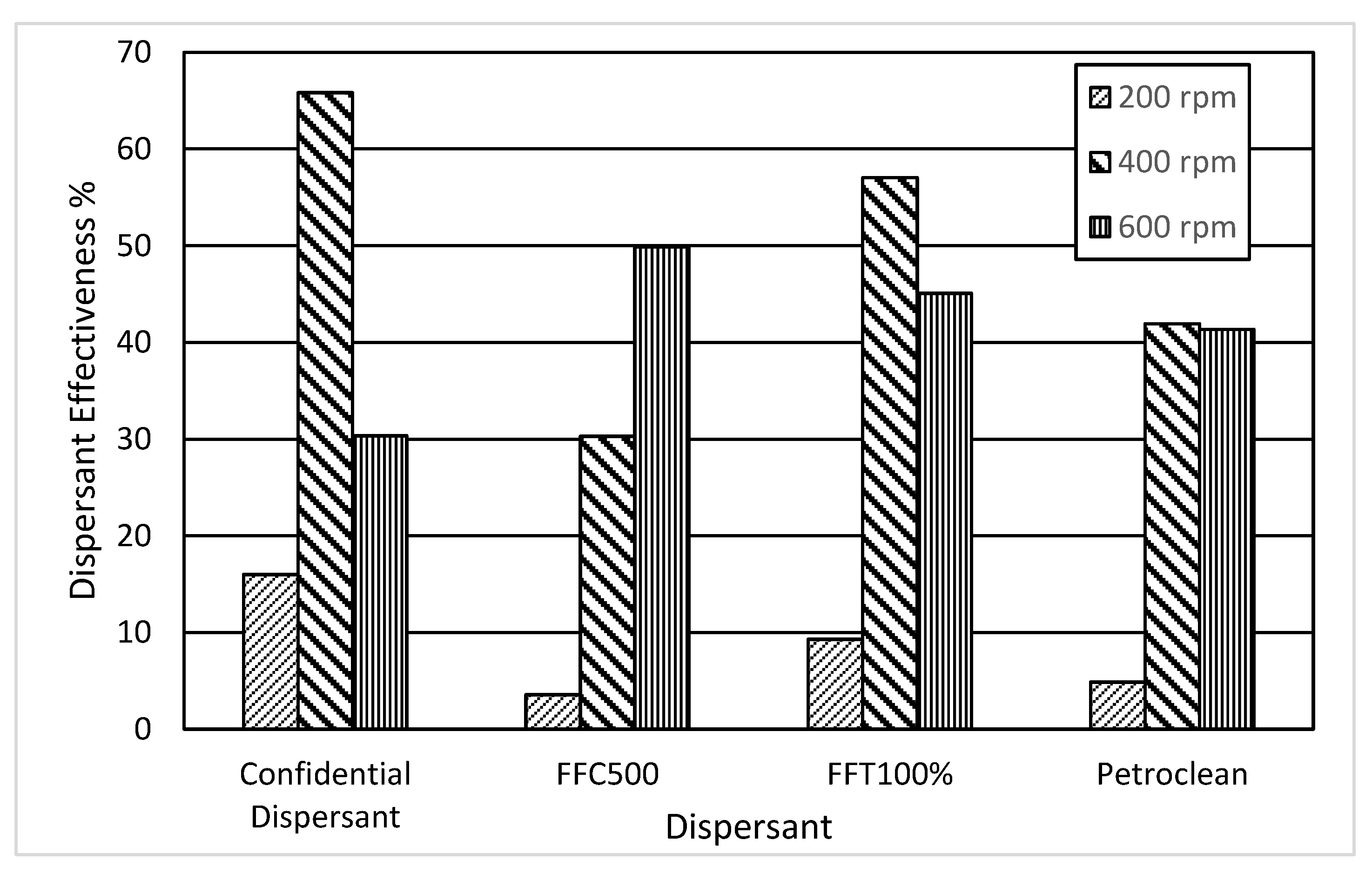
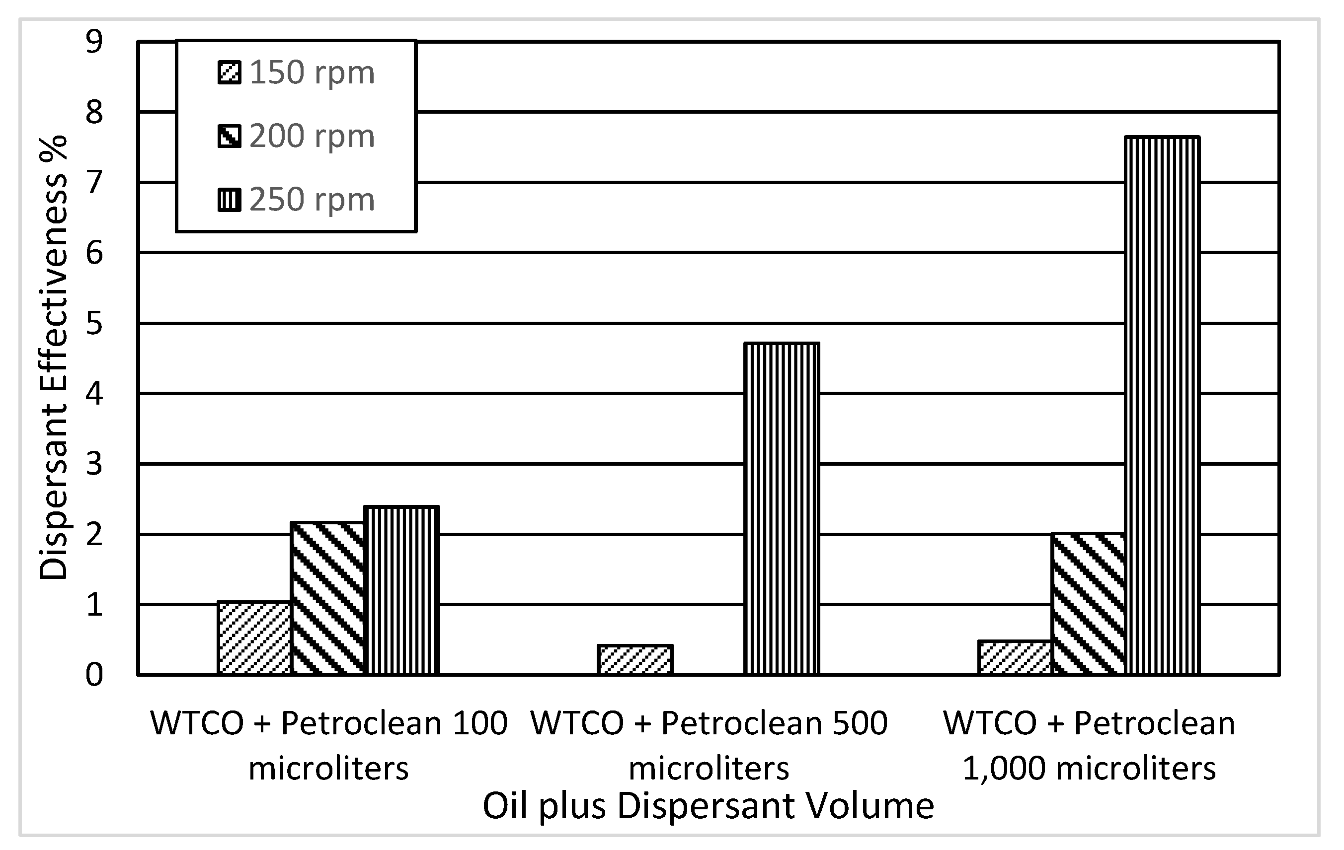
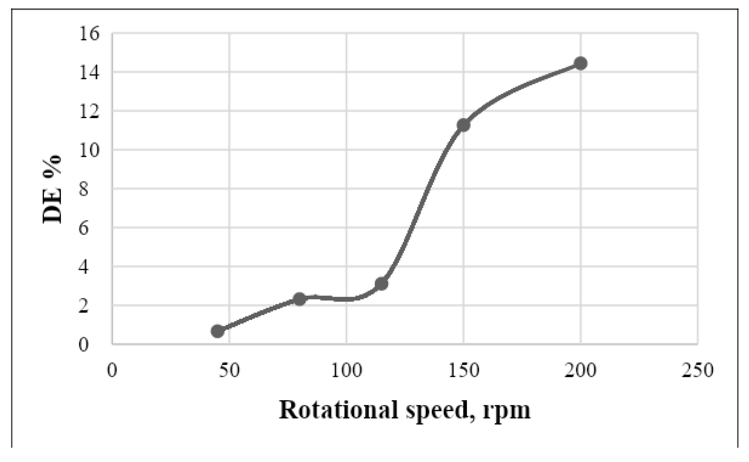
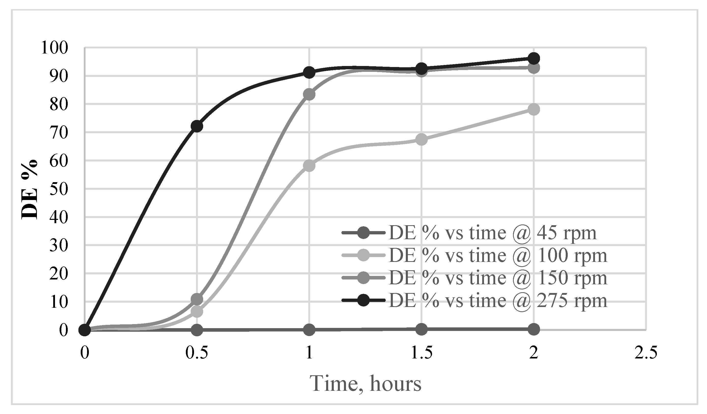
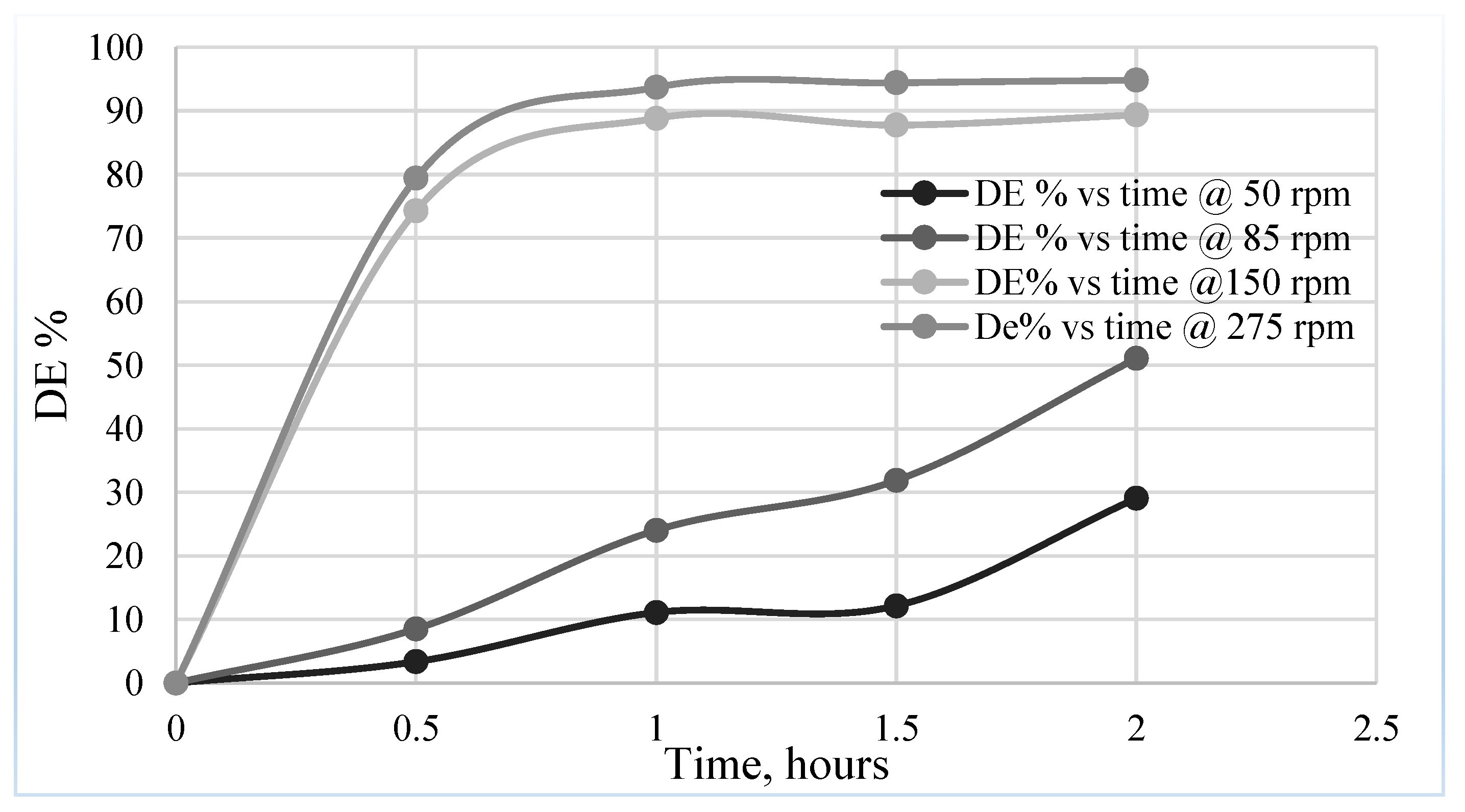
3.1.1. Dispersant Effectiveness

The effectiveness of dispersing WTCO while controlling paddle mixer rotational speed and dispersant formulation added with the oil phase at a ratio of 10 parts oil to 1 part dispersant on a volume basis is presented in Figure 2. This series of experiments was conducted in a 1000 mL baffled flask (see Figure 1), using a working volume of 360 mL. The greatest DE occurred with the confidential dispersant (DE = 66%) and the FFT100% dispersant (DE = 57%) at the 400 rpm speed. Significant DE (DE in the 30–70% range) occurred at the 400 and 600 rpm speeds, while only minimal DE (15% or less) occurred at the 200 rpm speed. The calculated energy dissipation values associated with these mixing speeds were 0.29 W/kg at 200 rpm 2.3 W/kg at 400 rpm, and 7.8 W/kg at 600 rpm. Very little dispersion (<10%) occurred when the energy dissipation was less than 1.0 (specifically 0.29), at the 200 rpm condition. A marine impeller was also tested in this series of experiments (data not shown), but was much less effective than the paddle impeller in the baffled flask.
The effectiveness of dispersing WTCO (100 to 1000 µL oil with Petroclean as dispersant) at three different flask orbital shaking speeds is shown in Figure 3. These experiments were conducted in a in a 250 mL Erlenmeyer flask with side spout (see Figure 1), using a working volume of 120 mL. The mixing involved orbital shaking of the flask at speeds of 150, 200, or 250 rpm, rather than stirring with a mixer inside the vessel, as occurred in the previous set of experiments. All DE levels were lower than 10% in this particular experiment, which is believed to be due to the relatively low rotational speeds and the fact that the mixing was accomplished without blade mixing of any type. At the shaking speed of 150 rpm, the low DE levels (1% or less) decreased as the volume of the oil/dispersant applied to the system increased from 100 to 1000 µL. At the shaking speed of 250 rpm, the DE levels increased from 2% to 7% as the volume of the oil/dispersant applied to the system increased from 100 to 1000 µL. The DE levels at 200 rpm (approximately 2%) in this set of experiments were generally consistent with the DE results with Petroclean dispersant presented in Figure 2. The Design Expert software was used to develop an empirical equation (Equation (18)) for the mass of oil dispersed (directly related to DE%) using the results from the full fractional factorial set of experiments, based upon the independent parameters mixing speed (A), volume of oil plus dispersant added (B), type of dispersant (C), and ratio of oil to dispersant (D). The equation originally included four first-order terms, six second-order terms mixed parameter terms, and the second-order parameter squared terms for A and B. The ANOVA table that resulted from this analysis is included as Table S5 (Supplemental Materials). The significant terms (p < 0.05) were A, B, C, A*B, A*D, and B*D; all others were not significant since their p-values were greater than 0.05.
Mass of oil = 19.06 + 14.33*A + 16.86*B + 2.36*C + 15.98*AB − 3.38*AD − 3.55*BD
In the third series of dispersant effectiveness experiments, the duration of the mixing period was utilized as a control parameter, along with the rotational speed of mixing of two different types of impellers (paddle and helical ribbon). Additionally, the experiments were carried out at two different scales, namely a laboratory scale using the 1000-mL baffled flask (working volume of 360 mL), followed by a pilot-scale container of volume 41 L, and working volume of 30 L. Additionally, the container sizes, mixing blade size, and mixer rpm were used to calculate power and energy dissipation for each experimental case according to the equations presented in Section 2, which were then correlated on a single graph of energy dissipation versus power of mixing. For the entirety of this set of experiments, Petroclean was used as the dispersant.
The first graph in this set of experiments presents (Figure 4) the DE levels as measured at five different mixing speeds (impeller mixing, 50 to 200 rpm) in the 1000 mL baffled flask. The results indicate relatively low but generally increasing DE levels, from less than 1% up to 14%, as the speeds rise from the 45 to 200 rpm. All results in this subset of experiments are for DE readings taken after 20 min of mixing.
The next two graphs (Figure 5 and Figure 6) present the time-based progression of DE levels at four different mixer speeds at the pilot scale using a 4-inch paddle impeller (Figure 5) and a 4.2-inch helical ribbon impeller (Figure 6). In these sub experiments, samples for determination of DE were collected at four time intervals, namely 0.5, 1.0, 1.5, and 2.0 h. In both cases, the DE rose abruptly at the higher speeds, and gradually at the lower speeds, except for the case of the lower speed of 45 rpm for the 4-inch paddle impeller, where the DE stayed at virtually zero for all time points measured. The final DE levels attained at the two highest speeds of 175 and 250 rpm were roughly all the same, at approximately 90%, regardless of mixer type. At the intermediate speeds of 100 rpm (paddle) or 85 rpm (helical), the DE levels increased but in a different manner, abruptly (paddle) versus gradually (helical). The results observed at the shorter time point of 0.5 h are directly in line with the previous results presented in Figure 2 and Figure 3, as only low DE levels were achieved at mixing speeds of 100 rpm or lower, while quite high (90%) DE levels were achieved with mixing speeds above 150 rpm. Finally, Figure 7 presents a graph of the calculated average particle size, determined using Equation (1), as a function of mixing speed for all dispersant effectiveness data described above. The calculated particle sizes range from a low of approximately 200 μm for the highest speed at the lab scale (200 rpm) to approximately 5000 μm for the lowest speed (50 rpm) at the pilot scale with the helical impeller. An apparent disadvantage of the helical impeller indicated in Figure 7 is that its use results in a larger particle size as compared to the paddle impeller at the same rpm.
The final figure from this set of experiments depicts all of the DE results from Figure 4, Figure 5 and Figure 6 above, plotted as individual points on a graph of energy dissipation ε versus power of mixing (Figure 8). In this graph, four diagonal lines represent the values of energy dissipation and power at a range of mixing speeds (rpm values), as calculated from the equations presented in Section 2, for three cases of the laboratory scale, pilot scale paddle mixer, and paddle pilot scale helical mixer. Then, the individual DE results are plotted, with the DE levels notated per data point. This graph shows how the helical impeller is able to achieve high DE levels at lower power input values, as compared to the paddle impeller at the pilot scale.

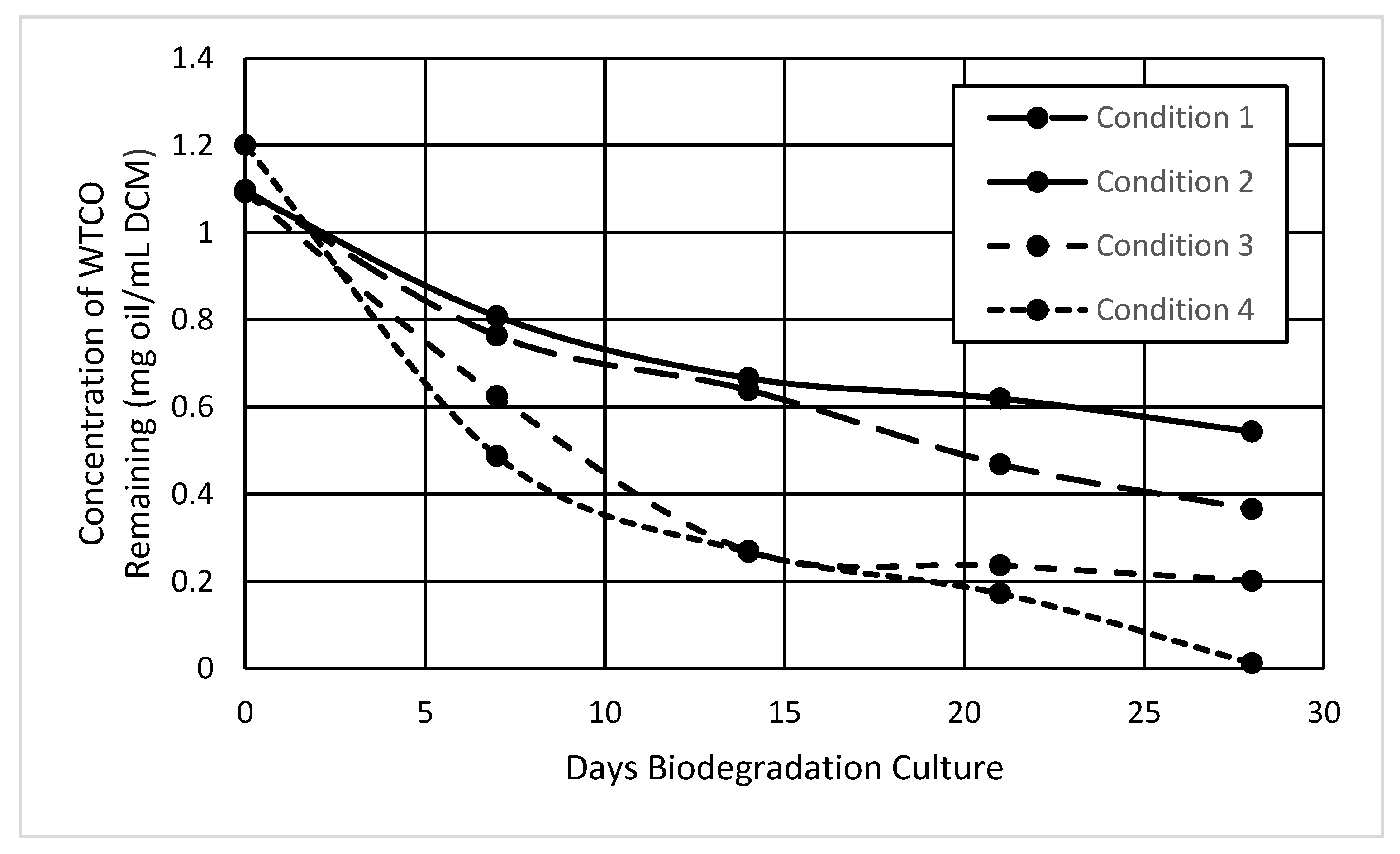
3.1.2. Biodegradation

A batch culture demonstrating biodegradation of WTCO under four test conditions is presented in Figure 9. In this series of experiments, the first three conditions included WTCO and the confidential dispersant as the oil/dispersant phase, along with the Oppenheimer formula as the petroleum-degrading microbial culture. The fourth condition included WTCO and the Oppenheimer formula, but no dispersant was included with the oil phase. Conditions 1 and 2 included mixing with the paddle impeller at 300 and 600 rpm during the up-front oil dispersion step, prior to commencement of the biodegradation culturing, while conditions 3 and 4 had no oil dispersing step at the beginning. The test condition that resulted in the greatest extent of biodegradation was the fourth condition, which did not include any dispersant formulation. This result suggests that perhaps this particular dispersant has a moderate negative effect upon hydrocarbon biodegradation activity. Nearly complete biodegradation of the dispersed oil was observed in this condition, while for the other three conditions, roughly 50 to 80% removal of the dispersed oil by biodegradation was accomplished.
The next two series of biodegradation experiments provided results very similar in nature to those shown in Figure 8. Thus, the results are shown only in table format in Table 2 and Table 3 below. In Table 2, the test conditions that were varied were the dispersant and the oil to dispersant ratio, as indicated in the first two columns of the table. All four conditions gave similar results for the extent of biodegradation (76% to 85% hydrocarbon removal) after culturing for a 21-day duration, with those using the Petroclean as dispersant indicating slightly greater biodegradation extent. These results are quite similar to the 21-day results for conditions 3 and 4 depicted in Figure 8. In this set of experiments, two controls with no bacterial culture added resulted in constant dispersed hydrocarbon levels throughout the entire 21-day period (data not shown).
In Table 3, the only test condition that was varied was the orbital shaking speed (55 to 200 rpm) used to disperse the oil for 20 min at the beginning of this biodegradation test. The orbital shaking speed used during the culturing step was 150 rpm for all conditions, while the other constants were the use of Petroclean as the dispersant, and the use of the Oppenheimer formula as the added bacterial culture. The results presented indicate a steady rise in the extent of WTCO biodegraded in step with the shaking rpm, with a large difference between the first two conditions of 50 and 100 rpm. In this set of experiments, two controls with no bacterial culture added resulted in constant dispersed hydrocarbon levels throughout the entire 21-day period.

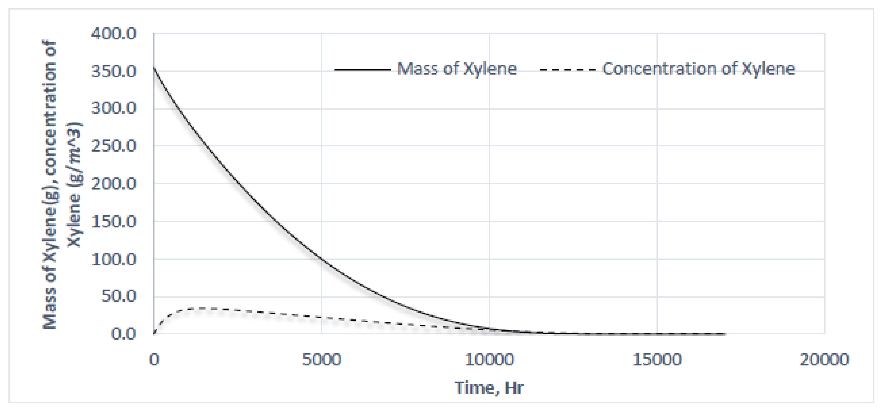
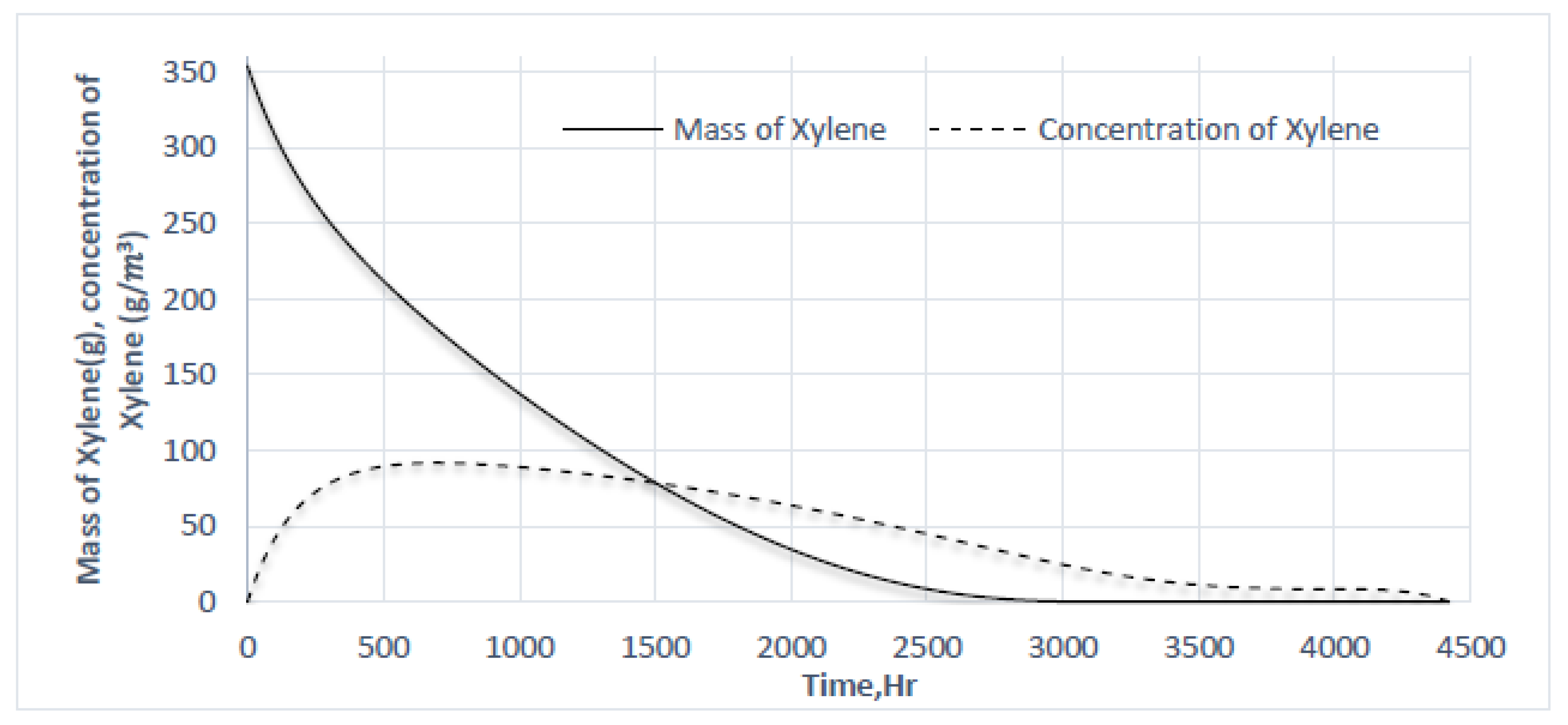
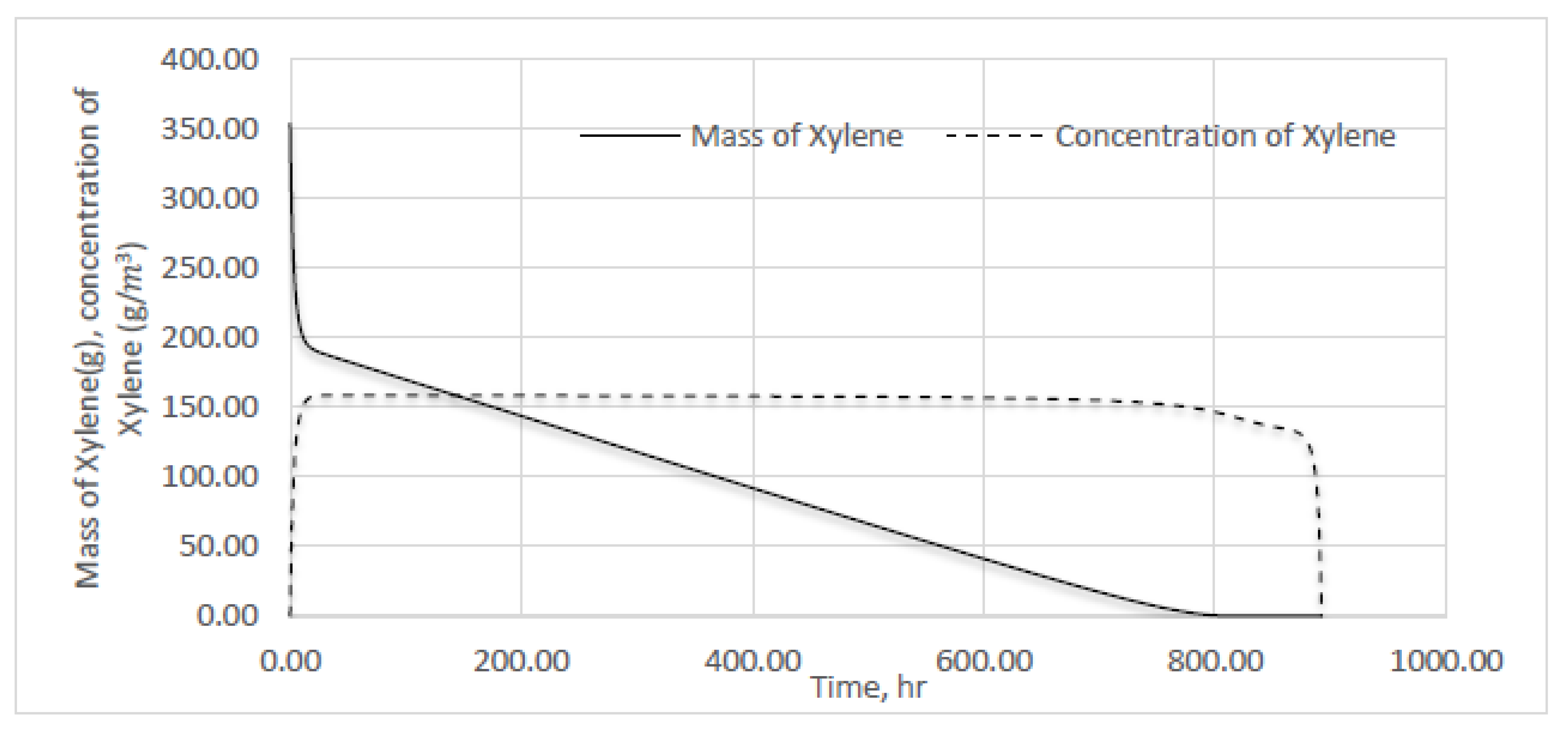
3.2. Modeling Results

All modeling results presented herein were completed using a single component, such as one of the four BTEX compounds, with the particle diameter serving as the independent parameter for each model run. The first results presented below are specifically for xylene, based on the equations and parameters presented in Section 2.2. The typical batch curves generated by the model for total mass MSx (grams) and dissolved concentration CSx (grams/m3) of xylene, for three dispersed phase particle sizes of 5000 µm, 2000 µm, and 200 µm, are shown in Figure 10, Figure 11 and Figure 12, respectively. In all cases, the model predicts a steady decline in the xylene mass M, and a rise and later fall in the dissolved xylene concentration, with different character depicted for the concentration curve, depending on the particle size. Large NAPL phase particles result in a lower dissolved phase concentration (Figure 10) over time, due to the limited amount of surface area for mass transfer of the NAPL particles in contact with the aqueous phase. Conversely, the dissolved concentration rises to the solubility limit in the case of the smaller NAPL phase particle size (Figure 12), due to the greatly increased surface area for mass transfer associated with this case. Figure 10, Figure 11 and Figure 12 also depict the batch time at which 99% of the original mass is biodegraded, with this value decreasing as the particle size decreases.
A summary graph of the time required to attain 99% biodegradation versus particle size for xylene, over the range of particle sizes of 6000 µm to 100 µm, is depicted in Figure 13. The data in this graph were developed using model runs with the mass transport from dispersed particles to the dissolved phase occurring only by diffusion. Below a particle size of 500 µm, the time period needed to reach 99% biodegradation levels is in the range of 500 to 1000 h. These biodegradation time periods are roughly consistent with the experimental biodegradation results presented in Figure 8 and Table 1 and Table 2 above. The qualitative agreement in biodegradation times between the experimental and modeling results suggests that perhaps the portion of WTCO dispersed and biodegraded in these experiments is predominantly lighter hydrocarbons of similar biodegradability (half-life values) as the xylene employed in the modeling.
The sensitivity of the results for the time period used to reach 99% biodegration as a function of variation in the biodegradation constant for xylene is shown in Figure 14. The first and last values shown in the figure represent the high end (168 h) and low end (672 h) of the range of biodegradation half-life values for xylene [16]. Over this range of biodegradation rate constants, the time to 99% biodegradation varies from 1200 h to 300 h.
Additional model runs for xylene were completed using advective transport (Equations (13)–(16)) as compared to diffusive transport (Equation (12)) only. The results presented in Figure 15 depict the time to 99% biodegradation as a function of advection velocity over the range from 0 to 5 m/s, for the two different particle sizes of 150 and 500 µm. The results indicate that the positive effect of advection mass transport is greater at the larger particle size of 500 µm (biodegradation time decreases from 940 h to 490 h), and much less for the smaller particle size of 150 µm (biodegradation time decreases only from 840 h to 740 h).
Finally, the variation in time to attain 99% biodegradation as a function of the range of reported biodegradation rate constants for all four BTEX compounds is presented in Figure 16 (xylene data only presented previously in Figure 14). The graph suggests that the biodegradation times are quite insensitive to the range of biodegradation rate constants for benzene and toluene, while the trend for ethylbenzene is quite similar to that for xylene. The difference between the BT versus EX compounds is expected to be related to their aqueous solubility values. Benzene and toluene each have a notably higher solubility in aqueous solution (1770 mg/L and 530 mg/L respectively) as compared to xylene and ethylbenzene (169 mg/L and 198 mg/L, respectively).

4. Discussion

The dispersant effectiveness results in both shake flasks (mixing by orbital shaking) and in the baffled flask (mixing with paddle mixer) indicate a certain level of mixing energy is needed to effect good dispersion or breakup of NAPL into particles in the bulk phase (Figure 2, Figure 3 and Figure 4). In these laboratory-scale environments, generally a mixing speed above 200 rpm is needed to achieve a desirable level of dispersion. At mixing speeds of 200 rpm or below, which corresponds with energy dissipation values of 1 or below at this scale, only low dispersant effectiveness results were obtained, specifically levels of 20% DE or lower. The dispersion tests performed at the pilot scale demonstrated improved NAPL breakup was achieved at lower mixing speeds (and lower energy dissipation levels), although it involved higher power input (Figure 8). The pilot scale results also indicated a significant difference in dispersion using the helical ribbon impeller versus the paddle impeller. The helical ribbon provided dispersion results comparable to the paddle impeller, but at energy dissipation levels that were roughly one order of magnitude lower (see Figure 8). Also at the pilot scale, dispersion was evaluated over 2 h. At the higher mixing speeds (150 and 275 rpm), high dispersion levels of 80 to 90% were achieved within 1 h, while at the lower mixing speeds in the range of 45 to 100 rpm, a slower and continually-increasing dispersion occurred out to 2 h. Similar results of increasing dispersion with time was observed in the work Pan et al. [6]. The dispersant effectiveness test detailed from the Code of Federal Regulations [7] is described for only small lab-scale testing volumes and only one time period of mixing. In this work, the size of testing and duration of mixing have been expanded for the purposes of evaluating dispersion as a possible oily sludge treatment method. These changes present challenges, such as obtaining a dispersed-phase-only sample when used at a larger scale, and the size of the mixing element as compared to the container of testing, which need to be adequately addressed by careful experimental planning if similar methods are used for larger scale testing. Estimates of the energy dissipation that occurs in the open ocean environment were also provided by Pan et al. in an experiment conducted in a lake in Ontario, where the mixing by wave action was estimated to represent an energy dissipation rate between 10−3 and 10−2 W/kg for the open water surface and between 1 and 10 W/kg for breaking waves [6]. The results depicted in Figure 6 and Figure 8 suggest that a helical mixer operated at a low to medium rotational speed may be effective at a full scale to effectively disperse NAPL oil material over time so as to feed an aqueous phase biodegradation process.
The comparison of the different dispersants used per the results presented in Figure 2 suggests that the confidential dispersant is the best and the Petroclean dispersant performed as least desirable. However, other results presented here suggest that the Petroclean can achieve high dispersant effectiveness results when the mixing time is extended beyond the originally prescribed 20 min (Figure 5 and Figure 6). These comparable outcomes are also implied by the biodegradation results presented in Table 2. The polynomial equation derived from the fractional factorial design experiment indicated the C term (type of dispersant) was significant; however, review of the p-values in Table S5 indicates that the type of dispersant term is not as highly significant as the first two terms; that is, the mixing speed (A) and volume of oil added to the system (B).
The biodegradation of dispersed oil in batch culture demonstrated oil removal, as measured by the difference from the dispersed oil remaining in the aqueous phase over a testing period of 21 to 28 days. The chemical makeup of the portion of WTCO dispersed into the bulk aqueous phase was not analyzed in this work; therefore, we are not able to define whether the portion of oil degraded was the lighter portion of the crude oil, although presumably that is the case. Regarding the biodegradation data presented in Figure 9, the fourth test condition, which did not include the confidential dispersant formulation as did the others, was the condition which indicated the greatest level of dispersed oil biodegradation. Other researchers have also reported hindered dispersed oil biodegradation apparently due to the presence of a dispersant Corexit, as compared to a condition with no dispersant added, under similar 35-day batch test conditions [4]. However, this effect is not consistent with other cases [5]. The dispersants Petroclean and FFT indicated 70 to 80% biodegradation levels at 21 days of culture in shake flasks (Table 2). The biodegradation extent was also positively enhanced by higher levels of mixing energy (Table 3), which is expected based on the higher mixing energy responsible for small disperse particle sizes.
The modeling presented herein is simplistic in that NAPL particle size is an input parameter rather than a calculated result of the model. Even so, the dissolution and biodegradation data presented by model runs conducted at different particle sizes qualitatively reflect the findings determined in the experimental work. In particular, the model results indicate a time frame of 300 to 1200 h (12 to 50 days) to attain biodegradation of 99% of an original xylene NAPL mass, while comparable endpoints from the experimental biodegradation tests were demonstrated by the attainment of 90% or greater biodegradation over 21 or 28 days (Figure 9 and Table 2 and Table 3). The additional result of interest arising from the modeling work is the minor contribution that advection may have, as compared to diffusion-only mass transport, on overall time required to achieve 99% biodegradation as a function of the particle size. The results indicated a very minimal effect on the time required to achieve 99% biodegradation for the 150 μm particle size, with a more pronounced effect of approximately a two-fold difference for the 500 μm particle size. This difference is expected to be due to the smaller total surface area for mass transfer associated with the larger particle size.

5. Conclusions

The results of the dispersant effectiveness test indicated that mixing with an intensity of approximately 150 to 200 rpm is necessary to achieve hydrocarbon dispersion of 80% or higher, using either the paddle or the helical ribbon impeller. The power levels calculated in using the helical ribbon impeller were five to ten-fold lower than that required for a similar sized paddle impeller, with similar dispersant effectiveness. The oil biodegradation tests conducted with dispersants and mixing in the same manner as the dispersant effectiveness test resulted in 50% to nearly 100% degradation over a duration of 21 to 28 days, with minor variations due to dispersant type and speed of mixing in the initial oil dispersion step. The modeling of the single component hydrocarbon dissolution from droplets and subsequent aqueous phase biodegradation indicated smaller dispersed phase droplet sizes promoted more efficient biodegradation, which supports the laboratory findings that greater mixing intensity is needed for effective dispersion, dissolution, and biodegradation.
The preliminary research findings of improved oil dispersion with higher levels of mixing energy, and use of different impeller types (helical ribbon akin to pond mixer type device), support the idea of implementing oil sludge biodegradation in a pond environment enhanced via dispersant and petroleum-degrading microbial consortia addition. However, the greatest challenge will likely be attaining the desired higher oil dispersion levels in a medium to large pond area without the need for an unreasonably high number of mixers. Future research directions will include further investigation of pilot and small full-scale mixing and oil dispersion using an impeller of the helical ribbon type that is used in commercial wastewater pond mixers, and concentrating on the ability to disperse NAPL to suitable particle sizes with reasonable power levels, and to provide adequate oxygen levels for aerobic biodegradation at operational scales larger than the 30-L pilot employed here. Additionally, the dispersing and biodegradation tests conducted in the future should incorporate means to assess the range of oil components dispersed or biodegraded, with particular interest in the fate of the heavier hydrocarbons present in a crude sample. Future work on the modeling portion of this investigation will include multicomponent dissolution and modeling using a population balance approach to represent a distribution of particles.

Supplementary Materials

The following are available online at https://www.mdpi.com/2076-3417/10/5/1659/s1, Table S1. Independent values for dispersant effectiveness tests conducted in 250-mL Erlenmeyer flasks; Table S2. Power number, Power consumed and energy dissipation at various rotational speeds-Lab scale with 2.5" paddle impeller; Table S3. Power number, Power consumed and energy dissipation at various rotational speeds-Pilot scale using 4" paddle impeller; Table S4. Power number, Power consumed and energy dissipation at various rotational speeds-Pilot scale using 4.2" helical ribbon impeller; Table S5. ANOVA table for fractional factorial analysis (see Equation (18) in text); Derivation for Equation (7).

Author Contributions

Dispersion effectiveness and biodegradation in baffled flask, N.A.; dispersion effectiveness and biodegradation in shake flasks, M.C.; dispersion effectiveness, energy dissipation, at laboratory and pilot scale, A.S.; modeling work for xylene, T.M.; modeling work for other BTEX compounds, S.R.; supervision and writing, M.A. All authors have read and agreed to the published version of the manuscript.

Funding

This research received no external funding.

Conflicts of Interest

The authors declare no conflict of interest.

References

  1. Hu, G.; Li, J.; Zeng, G. Recent development in the treatment of oily sludge from petroleum industry: A review. J. Hazard. Mater. 2013, 261, 470–490. [Google Scholar] [CrossRef] [PubMed]
  2. Rathi, V.; Yadav, V. Oil degradation taking microbial help and bioremediation: A review. J. Bioremediat. Biodegrad. 2019, 10, 460–465. [Google Scholar]
  3. Yateem, A.; Balba, M.T.; Al-Shayji, Y.; Al-Awadhi, N. Isolation and characterization of biosurfactant-producing bacteria from oil-contaminated soil. Soil Sediment Contam. 2002, 11, 41–55. [Google Scholar] [CrossRef]
  4. Rahsepar, S.; Smit, M.P.; Murk, A.J.; Rijnaarts, H.H.; Langenhoff, A.A. Chemical dispersants: A biodegradation friend or foe? Chemosphere 2016, 108, 113–119. [Google Scholar] [CrossRef] [PubMed]
  5. Overholt, W.A.; Marks, K.P.; Romero, I.C.; Hollander, D.J.; Snell, T.W.; Kostka, J.E. Hydrocarbon degrading bacteria exhibit a species specific response to dispersed oil while moderating ecotoxicity. Appl. Environ. Microbiol. 2015. [Google Scholar] [CrossRef] [PubMed] [Green Version]
  6. Pan, Z.; Zhao, L.; Boufadel, M.C.; King, T.; Robinson, B.; Conmy, R.; Lee, K. Impact of mixing time and energy on the dispersion effectiveness and droplets size of oil. Chemosphere 2017, 166, 246–254. [Google Scholar] [CrossRef] [PubMed]
  7. Office of the Federal Register. Title 40: Protection of Environment. In Code of Federal Regulations (CFR); Office of the Federal Register: Washington, DC, USA, 2010; pp. 300–399. [Google Scholar]
  8. Hinze, J. Fundamentals of the Hydrodynamic Mechanism of Splitting in Dispersion Processes; Royal Dutch Shell-Laboratory: Delft, The Netherlands, 1955. [Google Scholar]
  9. Calabrese, R.V.; Chang, T.P.K.; Dang, P.T. Drop Breakup in Turbulent Stirred-Tank Contactors. Part I: Effect of Dispersed-Phase Viscosity. AIChE J. 1986, 32, 657–666. [Google Scholar] [CrossRef] [Green Version]
  10. Chen, H.T.; Middleman, S. Drop Size Distribution in Agitated in Liquid-Liquid Systems. AIChE J. 1967, 13, 989–995. [Google Scholar] [CrossRef]
  11. Shinnar, R.; Church, J.M. Statistical Theories of Turbulence in Predicting Particle Size in Agitated Dispersions. Ind. Eng. Chem. 1960, 52, 253–256. [Google Scholar] [CrossRef]
  12. Wang, C.Y.; Calabrese, R.V. Drop Breakup in Turbulent Stirred-Tank Contactors. Part II: Relative Influence of Viscosity and Interfacial Tension. AIChE J. 1986, 32, 667–676. [Google Scholar] [CrossRef] [Green Version]
  13. Kamei, N.; Hiraoka, S.; Kato, Y. Power correlation for paddle impellers in spherical and cylindrical agitated vessels. Kagaku Kogaku Ronbunshu 1995, 21, 41–48. [Google Scholar] [CrossRef] [Green Version]
  14. Kamei, N.; Hiraoka, S.; Kato, Y. Effects of impeller and baffle dimensions on power consumption under turbulent flow in an agitated vessel with paddle impeller. Kagaku Kogaku Ronbunshu 1996, 22, 255–256. [Google Scholar] [CrossRef] [Green Version]
  15. Furukawa, H.; Kato, Y.; Inoue, Y.; Kato, T.; Tada, Y.; Hashimoto, S. Correlation of power consumption for several kinds of mixing impellers. Int. J. Chem. Eng. 2012. [Google Scholar] [CrossRef] [Green Version]
  16. Howard, P.H.; Boethling, R.S.; Jarvis, W.F.; Meylan, W.M.; Michalenko, E.M. Handbook of Environmental Degradation Rates; Lewis Publishers: Chelsea, MI, USA, 1991. [Google Scholar]
  17. GSI Chemical Database. Available online: www.gsi-net.com/en/publications/gsi-chemical-database.html (accessed on 1 May 2019).
Figure 1. Glassware and mixers used for laboratory dispersant effectiveness and biodegradation testing: (a) 250-mL Erlenmeyer flask used with mixing by orbital shaking; (b) 1000-mL baffled flask used with shaft-driven mixer; (c) paddle mixer; (d) helical ribbon mixer.
Applsci 10 01659 g001
Figure 2. Dispersant effectiveness for WTCO in a 1000-mL baffled flask using 2.5-inch paddle impeller at laboratory ambient temperature (approximately 25 °C) and a 10:1 oil to dispersant ratio.
Applsci 10 01659 g002
Figure 3. Dispersant effectiveness for WTCO in 250-mL Erlenmeyer flask with orbital shaking and at a laboratory ambient temperature of approximately 25 °C (there is no 200 rpm bar in the “WTCO + Petroclean 500” category due to fractional factorial design of this experiment (see Table S1)).
Applsci 10 01659 g003
Figure 4. Dispersant effectiveness in a 1000-mL baffled flask (lab scale) at five different impeller 2.5-inch diameter) speeds at the laboratory ambient temperature (approximately 25 °C). (Power number results for this test are included in Table S2).
Applsci 10 01659 g004
Figure 5. Dispersant effectiveness at the pilot scale (30 L) using a 4-inch paddle impeller at the laboratory ambient temperature (approximately 25 °C). (Power number results for this test are included in Table S3).
Applsci 10 01659 g005
Figure 6. Dispersant effectiveness at the pilot scale (30 L) using a 4.2-inch helical impeller at the laboratory ambient temperature (approximately 25 °C). (Power number results for this test are included in Table S4).
Applsci 10 01659 g006
Figure 7. Calculated dispersed oil particle sizes as a function of mixing speed.
Applsci 10 01659 g007
Figure 8. Dispersant effectiveness results plotted on a graph of energy dissipation of mixing versus power at the laboratory and pilot scales.
Applsci 10 01659 g008
Figure 9. Dispersant effectiveness in the 250-mL Erlenmeyer flask at four different orbital shaking speeds. Condition 1: WTCO, confidential dispersant, and Oppenheimer formula, mixing at 300 rpm during oil dipsersion; Condition 2: WTCO, confidential dispersant, and Oppenheimer formula, mixing at 600 rpm during oil dipsersion; Condition 3: WTCO, confidential dispersant, and Oppenheimer formula, no mixing in oil dispersion step; Condition 4: WTCO and confidential dispersant only, no mixing in oil dispersion step. All biodegradation tests were conducted at room temperature (nominally 25 °C).
Applsci 10 01659 g009
Figure 10. Mass and concentration of xylene particles with Dp = 5000 μm.
Applsci 10 01659 g010
Figure 11. Mass and concentration of xylene particles with Dp = 2000 μm.
Applsci 10 01659 g011
Figure 12. Mass and concentration of particles of xylene with Dp = 200 μm.
Applsci 10 01659 g012
Figure 13. Particle size vs. time for xylene to reach 99% biodegradation.
Applsci 10 01659 g013
Figure 14. Kr vs. Time for xylene to reach 99% biodegradation (Dp = 500 μm).
Applsci 10 01659 g014
Figure 15. Velocity vs. time for xylene to reach 99% biodegradation.
Applsci 10 01659 g015
Figure 16. BTEX comparison at 500 µm with respect to various biodegradation rates.
Applsci 10 01659 g016
Table 1. Constant factors used in oil droplet size (Sauter diameter) prediction.
ParameterSymbolValue
Bulk phase densityρc998 kg/m3
Disperse phase densityρd821 kg/m3
Dispersed phase viscosityμd0.005 Pa-sec
Interfacial tensionσ0.03 N/meters
Table 2. Biodegradation extent for 250 mL shake flask cultures.
DispersantOil/Dispersant Ratio% Oil Biodegraded at 21 Days
Petroclean10:185.4
Petroclean10:282.8
FFT 7%10:178.6
FFT 7%10:276.3
Table 3. Biodegradation extent for 250-mL shake flask cultures.
Orbital Shaking Speed 1% Oil Biodegraded at 21 Days
5048
10083
15093
20099
1 speed for dispersing step only. During biodegradation culture duration, orbital shaking was at 150 rpm.

