Article

Delimitation of Agricultural Areas with Natural Constraints in Greece: Assessment of the Dryness Climatic Criterion Using Geostatistics

by
Konstantinos X. Soulis
1,*,
Dionissios P. Kalivas
2 and
Costas Apostolopoulos
3
1
Division of Water Resources, Department of Natural Resources Management and Agricultural Engineering, Agricultural University of Athens, 11855 Athens, Greece
2
Division of Soil Science and Agricultural Chemistry, Department of Natural Resources Management and Agricultural Engineering, Agricultural University of Athens, 11855 Athens, Greece
3
Evaluation and Institutional Support Unit, Managing Authority for RDP 2014–2020, Ministry for Rural Development and Food, 10441 Athens, Greece
*
Author to whom correspondence should be addressed.
Agronomy 2018, 8(9), 161; https://doi.org/10.3390/agronomy8090161
Submission received: 16 July 2018 / Revised: 10 August 2018 / Accepted: 21 August 2018 / Published: 23 August 2018

Abstract

:
The Less Favored Areas (LFAs) scheme has existed in various forms since 1975 and it is a broad mechanism supporting rural development in agricultural areas with natural constraints (ANC). Within the programme period 2014–2020, the European Commission developed a common set of biophysical criteria (soil, climate, and terrain) to meet the requirement for a robust and harmonized approach of delimiting ANC throughout the EU Member States. Soil and terrain criteria can be derived directly from soil maps using geospatial analysis techniques based on the provided guidelines. However, the assessment of climatic criteria can be challenging especially in regions characterized by increased spatial variability and data scarcity. In this paper, the assessment of the dryness climatic criterion in a data-scarce region (Greece) as well as the challenges, limitations, and solutions are presented. Daily data-series from 140 meteorological stations for a 30-year reference period were analyzed and the spatial distribution of the precipitation and the potential evapotranspiration for each year were estimated in order to make the final assessment of the dryness criterion. Climate variability and the presence of trends were investigated as well. The obtained results indicated that most of the utilized agricultural area is affected by dryness due to a combination of low precipitation and high evapotranspiration rates. The extreme spatial variability especially in precipitation was also highlighted. An important temporal variability was observed as well, including indications of decreasing trends in precipitation and aridity index. Climate variability and possible trends should be investigated in more detail using longer time series in order to evaluate their impact in agricultural production.

1. Introduction

The necessity of maintaining agricultural activity in less favored areas (LFAs) recognized since the beginning of the Common Agricultural Policy (CAP) of the European Union (EU) focuses on improving the viability of agriculture in areas with natural constraints [1,2]. The LFAs scheme is a major element of the EU Rural Development Policy and has existed in various forms since 1975 as a broad mechanism supporting rural development in agricultural areas with natural constraints (ANCs) [3,4]. Furthermore, the need for innovative strategies for the sustainable development of LFAs in order to promote environmental protection, social equity, and economic growth is recognized in many studies [5,6,7,8].
In 2003, the European Court of Auditors recommended that the delimitation of LFAs should be based on a set of common biophysical criteria rather than the socio-economic criteria on which the previous scheme was based [1,4,9]. Several studies were conducted in order to identify a set of common biophysical criteria capable of indicating the overall suitability of land for agriculture for the delimitation of LFAs in Europe, as well as several studies reviewing the various proposals [1,4,9,10,11,12,13,14,15,16,17,18]. Accordingly, the European Commission developed a common set of biophysical criteria (i.e., soil, climate, and terrain) to meet the requirement for a robust and harmonized approach of delimiting areas that experience natural constraints to agriculture throughout the EU Member States [9,10].
The most recent updated guidelines for applying common soil, climate, and terrain criteria to identify agricultural areas with natural constraints as set out in the EU Regulation 1305/2013 on support for rural development by the European Agricultural Fund for Rural Development (EAFRD) and repealing Council Regulation (EC) No 1698/2005 were published in 2016 [19].
The criteria are based on the “problem-land approach” [19,20,21]. The eight biophysical criteria developed for identifying significant natural constraints to agriculture in Europe are divided in climate criteria (Low Temperature, Dryness), climate and soil criteria (Excess Soil Moisture), soil criteria (Limited Soil Drainage, Unfavorable Texture and Stoniness, Shallow Rooting Depth, Poor Chemical Properties), and terrain criteria (Steep Slope). However, in countries or regions for which particular criteria are not relevant, they do not need to be calculated. Criteria are assessed according to the agronomic law of the minimum. More details are provided by Terres et al. [19]. Finally, it should be noted that the above criteria concern “natural” soil and climate conditions. Therefore, when natural conditions have been improved (e.g., through drainage, irrigation or other techniques), the corresponding areas should be excluded as the natural constraints have been overcome.
Previous studies investigated the assessment of soil and terrain criteria and described the data requirements and geospatial analysis techniques as well as possible challenges and limitations [2,16,22,23,24]. The assessment of climatic criteria can be also particularly challenging especially in regions characterized by increased spatial variability and data scarcity, while the obtained results are sensitive to data availability and quality as well as to interpolation methods and parameters [17,19,25,26].
A key characteristic of the South European countries and especially the Mediterranean countries is the huge spatial variability of meteorological conditions within short distances due to the steep relief, the long coast lines, and the great number of islands and peninsulas [25,27,28]. At the same time, in most cases the meteorological information available is scarce compared to other EU countries and limited to lower altitudes and/or coastal locations [25,29]. Therefore, this information cannot describe the rates of change in precipitation and temperature with respect to elevation and the strong spatial variability of the climate as influenced by elevation, relief, and advective processes [30]. Furthermore, some of the weather variables required for the estimation of potential evapotranspiration (ETo) such as wind speed and solar radiation are often lacking or are of low or questionable quality [31,32,33]. Especially, in the case of Greece, there is a vast spatial variability of both precipitation and potential evapotranspiration [26,34,35,36].
In this context, the assessment of the dryness climatic criterion using geographical information systems (GIS) and kriging interpolation techniques in a data-scarce region (Greece) are being presented. The main objective of this study is to analyze the most important challenges and limitations and to identify feasible solutions for the delimitation of agricultural areas subject to constraints due to dryness. Furthermore, climate variability and the presence of trends in the meteorological time series that may affect agricultural production and water resources availability at the future were investigated as well.

2. Materials and Methods
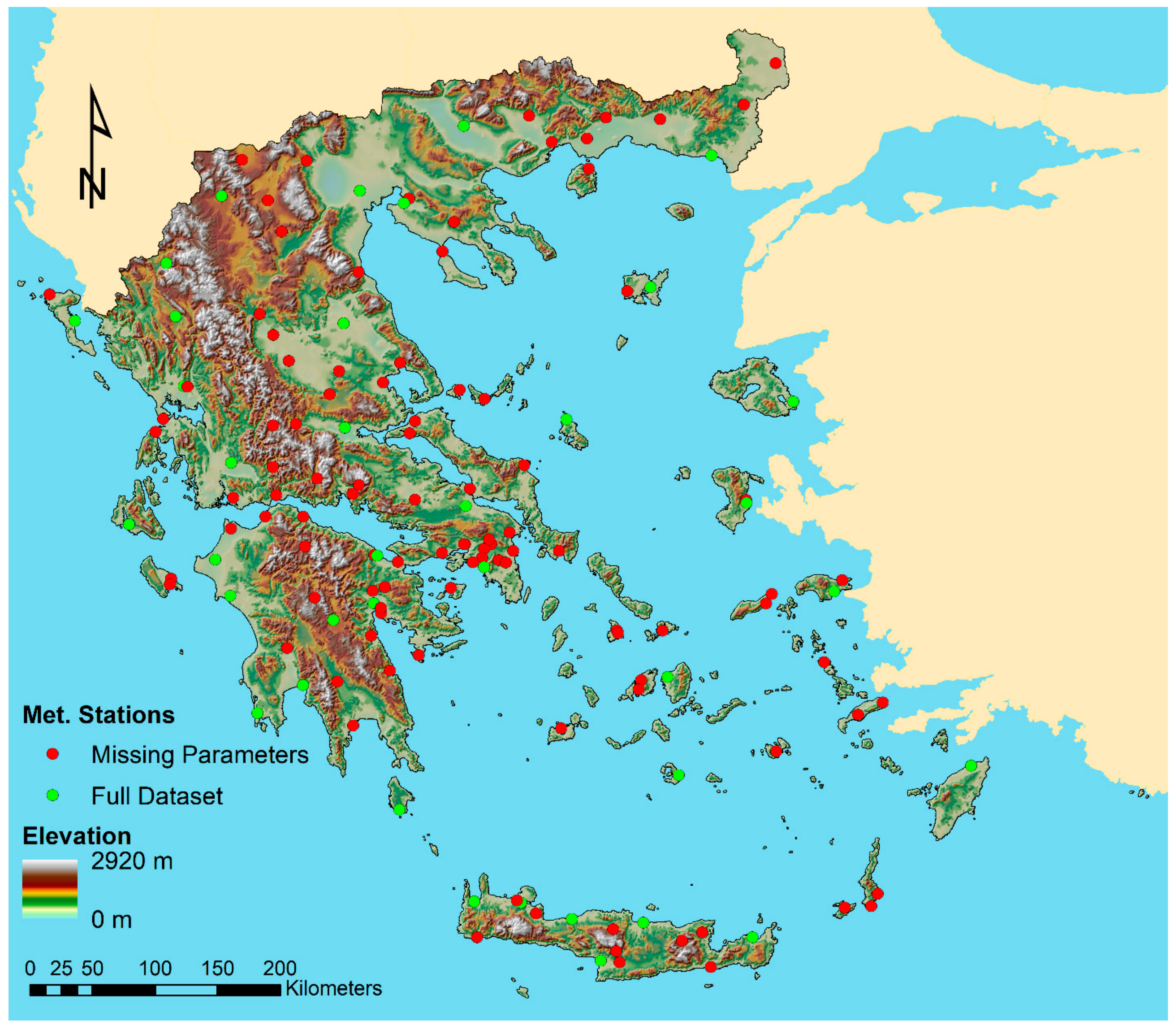
2.1. Data

The required climate data comes from the Hellenic National Meteorological Service (HNMS) [37], which is the National Service responsible to cover all the meteorological and climatological data needs of Greece. A total of 140 meteorological stations distributed all over the country were used (Figure 1). The density of meteorological stations is 1 station per 950 km2 and it can be considered adequate according to the international standards. However, Greece is characterized by a vast spatial variability of meteorological conditions in contrast to the relatively small size of the country (e.g., the annual precipitation depth ranges from well above 2000 mm/year at the higher elevation at the northwest to well below 500 mm/year at the southeast of the country [26,36]), which can be attributed to its steep relief including a massive sierra with a north-south direction dividing the mainland of the country, as well as its very long shoreline (Figure 1). Accordingly, possible limitations could be the variability of meteorological stations density across the country and the underrepresentation of higher elevations as most meteorological stations are located at lower altitudes (Figure 1).
Another important issue is that most of the 140 meteorological stations’ data-series had big gaps or didn’t record all the required weather parameters. As an example, only 37 meteorological stations provided solar radiation or sunshine hour data (Figure 1) and only these stations had adequate completeness and verified data quality by HNMS [37].
According to the EC guidelines [19], the recommended World Meteorological Organization’s (WMO) reference climatic period should be used. The current climate reference period in use by WMO consists of 30 years from 1 January 1961 to 31 December 1990. However, it is also suggested that it is possible to adapt the reference period to following a “rolling” set of 30 year, updated every 10 years depending on best available datasets. Based on the above and considering the best available meteorological data series in the meteorological stations of the study area, in this application the reference climatic period consists of 30 years from 1 January 1971 to 31 December 2000.
The data used in this study were daily time-series of precipitation (P) as well as daily time series of the required parameters for the estimation of potential evapotranspiration (ETo) with the FAO Penman–Monteith method [38], which are minimum, maximum, and mean temperature (Tmin, Tmax, and Tmean), mean relative humidity (RH), wind speed at 2 m height (WS), and solar radiation (Rs) or alternatively sunshine hours (SH).
In addition to the meteorological data, a digital elevation model of Greece provided by Shuttle Radar Topography Mission (SRTM) [39] was also used (Figure 1) as a secondary dataset in the geostatistical methods applied (cokriging). The spatial data of the Utilized Agricultural Area (UAA) were also used. The data were obtained by the Integrated Administration and Control System (OPEKEPE) [40] in the form of vector files with scale 1:10,000.
Finally, administrative boundaries (water districts, local administrative units) that were also used in the current analysis, were obtained by the Hellenic Statistical Authority [41] and by the Greek Public Open Geodata Service [42].

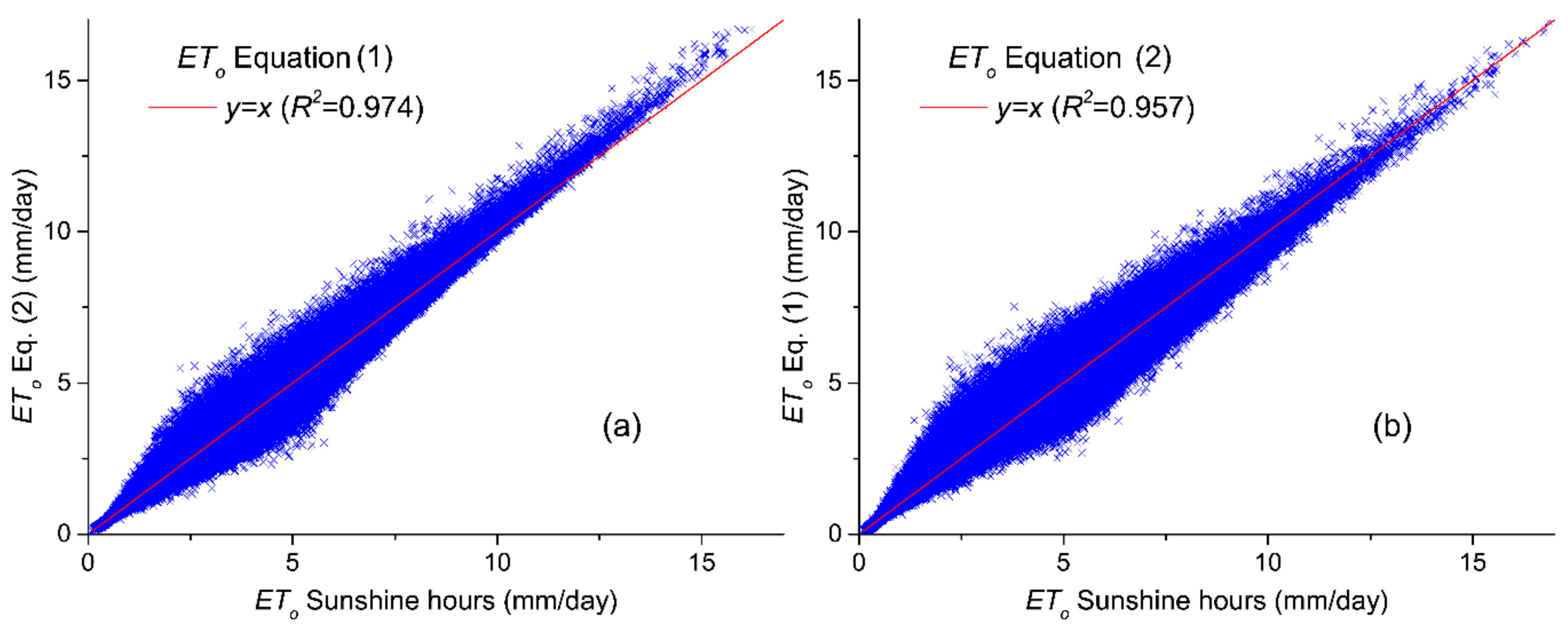
2.2. Meteorological Data Processing

The first step of this analysis was the assessment of the available datasets for integrity and consistency. As it was explained in more detail in the previous section, most of the 140 meteorological stations’ data series had big gaps or did not record all the required weather parameters (Figure 1). A possible option would be the use of only the stations having full datasets (all the required parameters), adequate completeness, and verified data quality. However, as can be seen in Figure 1, very few of the available stations meet these criteria. Consequently, the density of meteorological stations would not meet the minimum requirements according to the international standards and more important, the remaining stations would not be able to describe the vast spatial variability of meteorological conditions. A second possible option would be the use of alternative simplified ETo estimation formulas requiring for example only temperature data [43] or temperature and relative humidity data [44]; however, the specified EC guidelines [19] dictated the use of the FAO Penman–Monteith method [38].
Accordingly, in order to address the abovementioned problems of the available data series, a semi-automatic supervised data quality testing and gap filling algorithm was developed using MS Excel VBA in order to be able to process the huge dataset in reasonable time. The algorithm read the available data from the ASCII files of each station, created the data series for each parameter, identified gaps, and reported obviously erroneous values. The absolute minimum and absolute maximum recorded values for each parameter were used as thresholds for the identification of erroneous values. Various other checks were also performed, such as minimum values higher than average values or maximum values lower than average values, negative precipitation, sunshine hours or wind speed values etc. Marked erroneous values were manually examined in order to explore possible easy ways of correcting them in order to avoid the loss of precious data. As an example, stations with misplaced data values were identified and corrected or in cases that only the minimum value of a parameter was missing it was estimated based on the maximum and the average value and so on. Finally, the remaining gaps were filled using data from the three nearest stations based on the Inverse Distance Weight (IDW) method with a power of 1 and considering precipitation and temperature lapse rates for precipitation and temperature data respectively. Here, it should be noted that other alternative gap filling methods such as autoregressive models or artificial neural networks could be possibly used in order to avoid the problem of using spatial interpolation twice; first for gap filling and then for gridded surfaces generation. However, in this study, the approach used was the only feasible alternative given the available dataset limitations (e.g., large gaps, lack of autocorrelation for critical parameters like precipitation) as well as the limitations posed by the requirements of the guidelines (e.g., daily time step, meteorological stations density).
Especially for the case of sunshine hour data, which are used for the estimation of solar radiation, the available data come only from 37 meteorological stations, while there were several gaps in the data series including periods without any data in most of the available stations. Therefore, in the case of missing sunshine hour data, the estimation of solar radiation was made using the following equation [33]:
R s k R s   R A ( T max T d e w ) 0.5
where Rs is the solar radiation, RA is s the extraterrestrial radiation, Tmax is the maximum temperature, Tdew is the dew point temperature and kRs is an empirical radiation adjustment coefficient which generally varies from 0.12 to 0.25 and with a conventionally adopted value of 0.17 [33].
This equation is based on a similar equation proposed Hargreaves and Samani [43]:
R s k R s   R A ( T max T min ) 0.5
where Tmin is the minimum temperature.
Both equations were calibrated and evaluated by comparing the ETo values calculated using solar radiation estimated by sunshine hour data with the ETo values calculated using solar radiation estimated using Equations (1) and (2) for all the data points that sunshine hours data were available (376,000 data points).

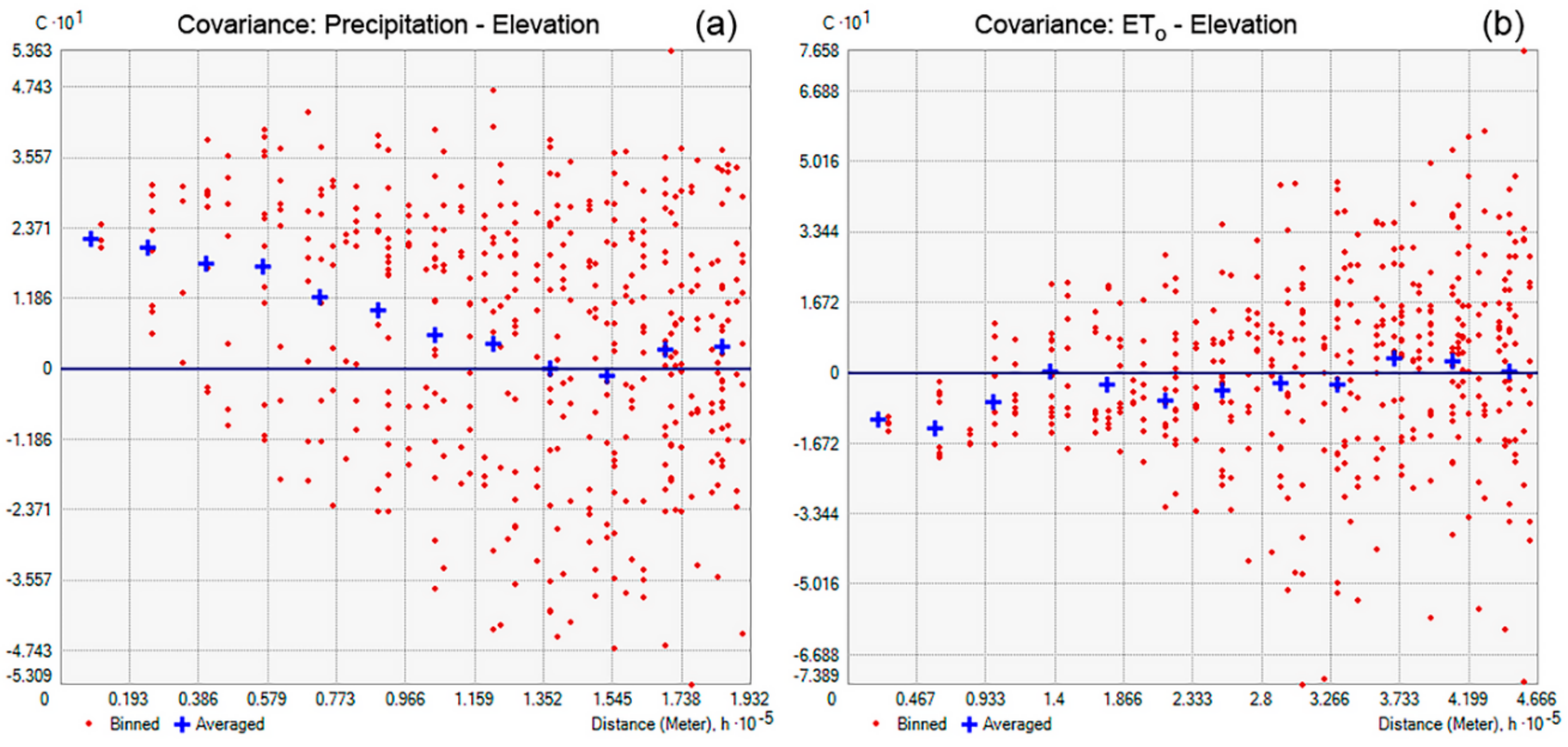
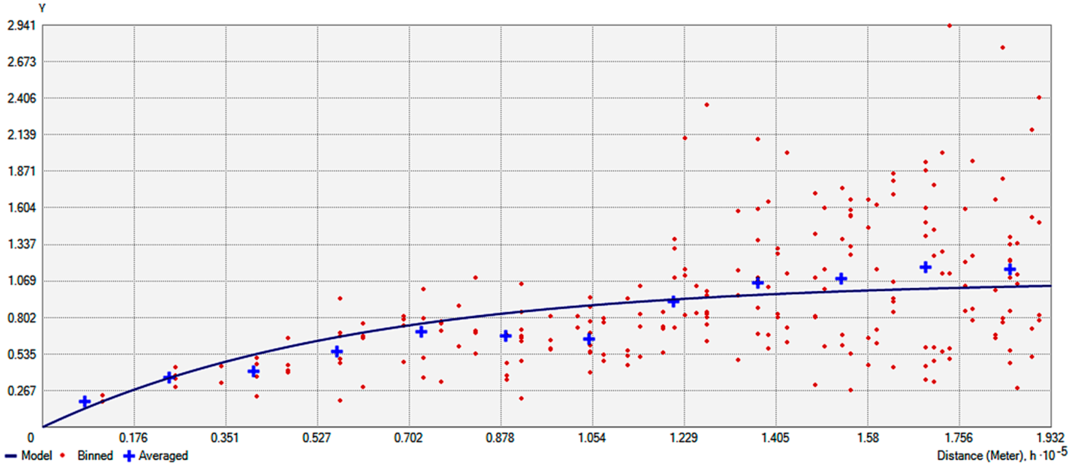
2.3. Spatial Interpolation

According to the EC guidelines [19], the calculation should be carried out with the annual totals of precipitation and of potential evapotranspiration for each year of the available data time series. Therefore, the daily grass reference evapotranspiration rates (potential evapotranspiration rates in relation to a living grass reference crop) were calculated using the FAO Penman–Monteith formula [38] for each day of the 30 years reference period and for each of the 140 meteorological stations. Then, the annual totals of P and of ETo for each year of the 30-year reference period and for each of the 140 meteorological stations were calculated. These calculated annual P and ETo data were then interpolated to produce the spatial distribution of the annual P and ETo depths for each year of the 30-years reference period. Considering the number and distribution of the meteorological stations as well as the steep relief of the studied area on one hand and the computational limitations on the other hand a grid resolution of 1000 m was chosen for the spatial interpolation in the study area.
In most similar applications the preferred spatial interpolation method is the kriging method [27,28,45,46,47,48] and this method is also proposed by the EC [19]. Especially for the case of Greece, which is characterized by vast spatial variability of P mainly due to its steep relief [26,34,35,36], the cokriging method may help to overcome the limitations posed by the meteorological stations density and the underrepresentation of higher elevations as most meteorological stations are located at lower altitudes. The cokriging method utilizes the covariance between two or more regionalized variables that are related to provide improved results when the main attribute of interest (e.g., precipitation) is sparse, but related with secondary information (e.g., elevation) which is abundant.
Therefore, the correlations between P and elevation and between ETo and elevation were examined in order to determine if the use of the cokriging method is justified. Arowolo et al. [49] reported that the use of additional secondary information such as the distance to the sea or longitude and latitude may further improve the obtained results. Accordingly, the possible use of the Euclidean distance to the nearest coast as secondary information was also investigated. However, including longitude and latitude as secondary information was not considered because P and ETo are not monotonically vary with respect to latitude and longitude.
The most suitable kriging method was also selected and the semivariogram/covariance modeling functions and parameters were evaluated. Then, using the selected interpolation parameters, two series of 30 interpolated layers each representing the spatial distribution of the annual P depth and the spatial distribution of the annual ETo depth for each year were created.
Finally, in order to test the accuracy of the interpolated surfaces cross-validation of all the obtained results was made. The statistical measures that were used are the mean error (ME), the root mean square error (RMSE), and the root mean square standardized error (RMSSE). The ME measures the bias of the prediction and should be close to zero for unbiased methods. The RMSE measures the average precision of the prediction and should be as small as possible. In RMSE the effect of each error is proportional to the size of the squared error; thus, RMSE is more sensitive to outliers. The RMSSE is a normalized statistical measure and facilitates the comparison between datasets or models with different scales. RMSSE values close to one indicate better performance.
All the above analysis was made using ESRI’s ArcGIS software package (version 10.5.1, Environmental Systems Research Institute, Redlands, CA, USA).

2.4. Dryness Climatic Criterion Assessment and Climate Variability

Using the interpolated P and ETo layers, the Aridity Index (AI) layers corresponding to each year of the 30-year reference period were calculated as follows:
A I = P E T o
Next, a raster layer representing the number of years, during which the dryness threshold is fulfilled (AI values ≤ 0.5 according to the guidelines [19]) was computed. Based on this layer, the areas subject to dryness were obtained by assigning 1 to values of the previous output raster with number of dry years > 20% according to the guidelines [19], and by assigning 0 to values ≤ 20%. The cells with a value of 1 are those areas subject to constraints due to dryness.
Finally, climate variability and the presence of trends in the time series were investigated. To this end, the areal P, ETo, and AI statistics were calculated for each of the 30 years and then their variability and possible trends were analyzed. Furthermore, the corresponding linear regression lines were fitted to the areal average of the annual P, ETo, and AI values and the corresponding 95% confidence bands were calculated. The significance of the difference of the corresponding slope values from 0 at the 0.05 confidence level was evaluated as well.

3. Results and Discussion

After the quality assessment, the correction, and the completion of the available datasets, a total of 140 meteorological stations (Figure 1) containing complete data-series for all the required parameters except from Rs were made available.
Concerning the evaluation of Rs, as can be observed in Figure 2a,b, both equations performed very well but Equation (1) performed slightly better (R2 = 0.974) than equation (2) (R2 = 0.957). Here it should be noted that the scatter observed in Figure 2 is created from a very small part of the 376,000 data points plotted in each graph and most of the data points are located near the x = y line. The calibrated kRs parameter values were 0.168 for Equation (1) and 0.195 for Equation (2). Therefore, Equation (1) was used to estimate solar radiation in the cases of missing sunshine hour data. The very high R2 values obtained and the overall performance of Equation (2), as can be clearly seen in Figure 2, indicate that the estimated ETo values for the cases of missing SH data are sufficiently accurate. The obtained kRs values were in the normal variation range for both equations. For the case of Equation (1) its value is very near to the conventional value of 0.17; however, for the case of Equation (2) it is a bit higher but well below 0.25.
Here, it should be noted that for locations having limited data availability or where the data quality is questionable, several simplified formulas requiring less parameters were developed from various researchers [33,43,44,50,51] and could simplify the procedure or in specific cases provide even better results [44]. However, the EC guidelines [19] dictate the use of FAO Penman–Monteith. This is an issue that should be more thoroughly studied and considered during the formulation of future guidelines.
After preparing the complete data-series for all the meteorological stations, the correlation of P and of ETo with elevation was investigated in order to examine if the use of the co-kriging method may provide improved predictions by taking advantage of the elevation data for each one of the parameters. In Figure 3a,b, the covariance between P and elevation and between ETo and elevation are plotted respectively. In Figure 3a a clear positive covariance can be observed for the case of precipitation. However, as can be seen in Figure 3b, for the case of ETo its covariance with elevation is weak. As it is also reported by Shi et al. [52] and Soulis [25], the relationship between ETo and elevation is complicated and it is very difficult to develop an algorithm for estimating spatially distributed ETo over mountainous regions. In contrast, it would be possible to consider the clearer relationships between meteorological parameters and topography (e.g., temperature-elevation, aspect-solar radiation, etc.) in order to improve the estimation of ETo spatial distribution [26,34,35,36]. However, in this case the calculation of ETo using the FAO Penman-Monteith formula and the spatial interpolation should be done in a daily time step. Accordingly, using this approach (i.e., first to estimate the spatial distribution of the meteorological parameters and then to compute ETo in spatially distributed form) would require the interpolation of the corresponding meteorological parameters for each day of the 30-year reference period requiring the calculation of 30 years × 365 days × 5 parameters = 54,750 layers. Accordingly, the use of co-kriging was neglected in the case of ETo. Nevertheless, it should be noted that any resulting inaccuracies are mainly expected in mountainous areas with very high elevations, which are not important for this analysis that concerns non-mountainous agricultural areas.
Arowolo et al. [49], in their study investigating spatial interpolation techniques to generate high-resolution climate surfaces for Nigeria, concluded that the use of kriging with longitude, latitude, elevation, and distance to coastline as external drifts provided improved results in the spatial interpolation of climate parameters. However, in the case of Greece the obtained results indicated that the spatial covariances between P and distance to the sea and between ETo and distance to the sea were weak, probably due to the complex topography of the country, which has a very long coastline and has many islands. Interestingly, the covariance between elevation and the distance to the sea was stronger, indicating that the two variables may not be independent in the case of Greece. However, it should be noted that more thorough study is needed to assess in more detail the effect of considering other external drifts on the spatial interpolation of climate parameters for the case of Greece due to its very complex geomorphology.
Following, the most suitable cokriging method was selected for the case of precipitation and the semivariogram/covariance modeling function and parameters were evaluated. The best results were obtained using the simple cokriging method. Furthermore, the exponential semivariogram model fitted adequately well in the studied dataset as can be seen in Figure 4. Finally, it was found that considering anisotropy improved the interpolation performance because it allowed taking into account the effect of the massive sierra with a north-south direction dividing the mainland of the country (Figure 1). It should be noted that the interpolation parameters evaluation was made using as a paradigm the 30 years average annual precipitation depths.
Following, using the selected interpolation parameters a series of 30 interpolated layers representing the spatial distribution of the annual precipitation depth for each year was created. The obtained results can be seen in Figure 5.
Finally, to test the accuracy of the interpolated surfaces cross-validation of all the obtained results was made. The obtained statistical measures were the following
  • Mean Error ranged between −52 and −64 mm
  • Root Mean Square Error ranged between 158 and 184
  • Root Mean Square Standardized Error ranged between 0.82 and 1.07
As can be seen in Figure 5, there is a vast spatial variability, which is present in both wet and dry years. The influence of the steep relief and especially of the massive sierra dividing the mainland of the country is also profound. Annual precipitation depths range from almost 2500 mm/year at the higher elevations at the northwest to almost 300 mm/year at the lower elevations at the southeast of the country and especially at the central Aegean islands. The presence of high temporal variability is also highlighted. As can be seen, there are some very wet years (e.g., 1979) and some very dry years (e.g., 1989). The big drought that lasted from 1988 to 1993 and caused major water shortages problems is also illustrated in Figure 5. What is also interesting is that the above observations are very similar with the general patterns presented in previous studies using different geostatistical methodologies and different datasets [26,36]. This fact supports the validity of the obtained results
For the case of ETo, the best results were obtained using the ordinary kriging method. Furthermore, the rational quadratic semivariogram model fitted adequately well in the studied dataset as can be seen in Figure 6. It was also found that in this case considering anisotropy did not improve the interpolation performance. It should be noted once again that the interpolation parameters evaluation was made using as a paradigm the 30 years average annual ETo.
Following, using the selected interpolation parameters a series of 30 interpolated layers representing the spatial distribution of the annual ETo depth for each year was created. The obtained results can be seen in Figure 7.
Finally, to test the accuracy of the interpolated surfaces cross-validation of all the obtained results was made. The obtained statistical measures were the following:
  • Mean Error ranged between −4 to −7.7 mm
  • Root Mean Square Error ranged between 72 to 124
  • Root Mean Square Standardized Error ranged between 0.84 to 1.52
As can be seen in Figure 7, there is profound spatial variability for the case of ETo as well. However, in this case the main differences are observed in the north-south axis. Specifically, annual ETo depths range from about 1800 mm/year at the southern part to about 900 mm/year at the northern part. The effect of the relief is also less obvious in this case. Temporal variability is less notable as well. In contrast with the case of P, in this case the obtained results have significant differences from a similar previous study [36], in which the relief had a dominant effect. Though, in that previous study, only temperature data were used in ETo estimation with the Hargreaves and Samani [43] method. The temperature lapse rate was also used in the spatial interpolation of temperature. In contrast, in this study the FAO Penman-Monteith method [38] using the complete set of parameters was used. The results of the current study are more in line with the findings of Shi et al. [51] and Soulis [25] reporting that the relationship between ETo and elevation is not clear.
The Aridity Index (AI) surfaces corresponding to each year of the 30-year reference period that were calculated using the interpolated P and ETo surfaces can be seen in Figure 8. As can be seen, the spatial and temporal patterns of AI mostly follow the spatial and temporal patterns of P. There are some very dry years that almost the entire country fells below the 0.5 threshold, while there are areas that fell below the 0.5 threshold in every year.
Based on the AI surfaces, a raster representing the number of years during which the dryness threshold is fulfilled (AI values ≤ 0.5) was computed as can be seen in Figure 9. The areas subject to dryness are the areas with a number of dry years greater or equal to 20% of the total reference period. The final results are illustrated in Figure 10, where the cells with a value of 1 represent those areas subject to constraints due to dryness. As can be observed, the areas subject to dryness are mainly located at the southeast part of the country and at lower elevations. Though, the eastern part of the country is also the most populated and where the biggest cities are located. Besides, the three most important and most productive plains are also located at the eastern part of the country (Thessaly, Thessaloniki, and Strymonas river valley). This fact leads to very high irrigation water needs at the eastern and mostly dry part of the country as it is also reported by Soulis and Tsesmelis [26], putting a lot of pressure on water resources.
As regards climate variability and the possible presence of trends in the time series, the temporal variability of the areal average of the annual P, ETo, and AI values as well as the corresponding linear regression lines and the corresponding 95% confidence bands are presented in Figure 11. As can be seen, P is characterized by high temporal variability, while for ETo and AI temporal variability is less notable. Furthermore, for the case of P a decreasing trend is observed with a slope of −6.57, which is significantly different from 0 at the 0.05 confidence level. In contrast, a slight increasing trend is observed for ETo with a slope of 0.27, which however, is non-significantly different from 0 at the 0.05 confidence level. As a result, a decreasing trend is also observed for AI with a slope of −0.0057, which is significantly different from 0 at the 0.05 confidence level. However, this preliminary analysis cannot provide safe conclusions due also to the short period studied (30 years). A more thorough analysis with longer data series is needed for this purpose. For example, Mimides et al. [53,54] using a long data series from stations in southern Bulgaria and northern Greece (1914–1994) observed the appearance of wet periods with periodic trends of about 20 years. However, Markonis et al. [55] reported that most regions in Greece show a decline in precipitation since 1950, an increase since 1980 and remain stable during the last 15 years. They also report that the significance of the observed decline is highly dependent to the statistical assumptions used and that change in time is strongly linked with the change in space (for scales below 40 years, relatively close regions may develop even opposite trends, while in larger scales change is more uniform).
As regards to the expected future conditions, Tolika et al. [56], considering twenty-two simulations from various Regional Climate Models (RCMs) reported that all the models estimated warmer and dryer conditions over the study area with the changes being larger in the continental than in the marine area of Greece. In terms of precipitation, a decrease up to −60% (A2 scenario) was estimated.
These trends may have important implications for agricultural production and could make water resources management in the country even more challenging. Accordingly, climate variability and possible trends should be investigated in more detail, using longer time series, in order to evaluate their impact in agricultural production.

4. Conclusions

In this paper the challenges, the limitations, and the solutions given for the assessment of the dryness climatic criterion using geographical information systems (GIS) and geostatistical techniques in a data-scarce region (Greece) were presented.
One of the most important challenges was the data quality testing and gap filling of the required meteorological parameters time series and especially for the case of solar radiation. For this purpose, two equations estimating Rs based on temperature and relative humidity data were tested and calibrated. Both equations performed very well and the calibrated kRs coefficient values were in the normal variation range for both equations.
The correlation of P and of ETo with elevation was also investigated in order to examine if the use of the cokriging method may provide improved prediction by taking advantage of the elevation data for each one of the parameters. A clear positive covariance was observed for the case of precipitation, while for the case of ETo the covariance between ETo and elevation is weak. For the case of precipitation, the best results were obtained using the simple cokriging method, the exponential semivariogram model, and considering anisotropy. For the case of ETo the best results were obtained using the ordinary kriging method and the rational quadratic semivariogram model.
A vast spatial and temporal variability of P was observed, while the influence of the steep relief and especially of the massive sierra dividing the mainland of the country is also profound. For the case of ETo there is also high spatial variability; however, in this case the main differences are observed in the north-south axis. The effect of the relief is also less obvious in the latest case and temporal variability is less notable.
The spatial and temporal patterns of aridity index mostly follow the spatial and temporal patterns of P. There are some very dry years that almost the entire country fells below the 0.5 threshold, while there are areas that fell below the 0.5 threshold in every year. The areas subject to dryness are mainly located at the southeast part of the country and at lower elevations, where the biggest cities and the most productive plains are located. This fact leads to very high irrigation water needs at the eastern and mostly dry part of the country putting a lot of pressure on water resources. Generally, most of the non-mountainous utilized agricultural area in Greece is affected by dryness due to a combination of low precipitation and high evapotranspiration rates. Considering also the findings of other studies estimating warmer and dryer future conditions over the study area it can be concluded that climate variability and possible trends should be also investigated in more detail, using longer time series, in order to evaluate their impact in agricultural production.
The present study may act as a paradigm for the assessment of climatic criteria in areas characterized by spatial variability and data scarcity.

Author Contributions

K.X.S., Conceptualization, Data curation, Formal analysis, Investigation, Methodology, Resources, Coding, Validation, Visualization, Writing, Review & editing; D.P.K., Project administration, Conceptualization, Methodology, Investigation, Resources, Supervision, Review & editing; C.A., Conceptualization, Methodology, Investigation, Resources, Review & editing.

Funding

This research was co-financed by the European Agricultural Fund for Rural Development and the Hellenic Ministry of Rural Development and Foods, Administrative Sector for Community Resources and Infrastructure, under the Technical Support measure of the Greek Rural Development Programme 2014–2020, grant number 320015.

Acknowledgments

The authors wish to sincerely thank the editor and the anonymous reviewers for their constructive comments and valuable suggestions.

Conflicts of Interest

The authors declare no conflict of interest.

References

  1. Eliasson, Å.; Jones, R.J.A.; Nachtergaele, F.; Rossiter, D.G.; Terres, J.; van Orshoven, J.; Le Bas, C. Common criteria for the redefinition of intermediate less favoured areas in the European Union. Environ. Sci. Policy 2010, 13, 766–777. [Google Scholar] [CrossRef]
  2. Erdogan, H.E.; Tóth, T. Potential for using the world reference base for soil resources to identify less favoured areas. Soil Use Manag. 2014, 30, 560–568. [Google Scholar] [CrossRef]
  3. Kučera, J.; Hlavsa, T. Agricultural land evaluation considering the Czech less favoured areas delineation. Acta Univ. Agric. Et Silvic. Mendel. Brun. 2017, 65, 1195–1204. [Google Scholar] [CrossRef]
  4. Schulte, R.P.O.; Fealy, R.; Creamer, R.E.; Towers, W.; Harty, T.; Jones, R.J.A. A review of the role of excess soil moisture conditions in constraining farm practices under Atlantic conditions. Soil Use Manag. 2012, 28, 580–589. [Google Scholar] [CrossRef]
  5. Střeleček, F.; Lososová, J.; Zdeněk, R. Economic results of agricultural holdings in less favoured areas. Agric. Econ. 2008, 54, 510–520. [Google Scholar] [CrossRef] [Green Version]
  6. Tsiaras, S.; Andreopoulou, Z. Sustainable development perspectives in a less favoured area of Greece. J. Environ. Prot. Ecol. 2015, 16, 164–172. [Google Scholar]
  7. Tsiaras, S.; Spanos, I. Tree crops cultivation. A sustainable alternative for the development of mountainous, less favoured areas. J. Environ. Prot. Ecol. 2017, 18, 271–281. [Google Scholar]
  8. Tsiaras, S.; Triantafillidou, E.; Katsanika, E. Green marketing as a strategic tool for the sustainable development of less favoured areas of Greece: Women’s agro-tourism cooperatives. Int. J. Electron. Cust. Relationsh. Manag. 2016, 10, 54–64. [Google Scholar] [CrossRef]
  9. Böttcher, K.; Eliasson, A.; Jones, R.; Le Bas, C.; Nachtergaele, F.; Pistocchi, A.; Ramos, F.; Rossiter, D.; Terres, J.M.; van Orshoven, J.; et al. Guidelines for Application of Common Criteria to Identify Agricultural Areas with Natural Handicaps; Office for Official Publications of the European Communities: Luxembourg, 2009; Volume 34. [Google Scholar]
  10. Asins-Velis, S.; Arnau-Rosalïn, E.; Romero-Gonzïlez, J.; Calvo-Cases, A. Analysis of the consequences of the european union criteria on slope gradient for the delimitation of “areas facing natural constraints” with agricultural terraces. Ann.-Anali Za Istrske Mediter. Studije-Ser. Hist. Et Sociol. 2016, 26, 433–448. [Google Scholar] [CrossRef]
  11. Castelo-Grande, T.; Augusto, P.A.; Fiúza, A.; Barbosa, D. Strengths and weaknesses of European soil legislations: The case study of Portugal. Environ. Sci. Policy 2018, 79, 66–93. [Google Scholar] [CrossRef]
  12. Ciglič, R.; Hrvatin, M.; Komac, B.; Perko, D. Karst as a criterion for defining areas less suitable for agriculture. Acta Geogr. Slov. 2012, 52, 61–98. [Google Scholar] [CrossRef] [Green Version]
  13. Gmeiner, P.; Hovorka, G. New delimitation of less favoured areas in Austria. J. Austrian Soc. Agric. Econ. 2011, 20, 63–72. [Google Scholar]
  14. Ivits, E.; Cherlet, M.; Tóth, T.; Lewińska, K.E.; Tóth, G. Characterisation of productivity limitation of salt-affected lands in different climatic regions of Europe using remote sensing derived productivity indicators. Land Degra. Dev. 2013, 24, 438–452. [Google Scholar] [CrossRef]
  15. Jarasiunas, G. Assessment of the agricultural land under steep slope in Lithuania. J. Cent. Eur. Agric. 2016, 17, 176–187. [Google Scholar] [CrossRef]
  16. Jarasiunas, G.; Kinderiene, I.; Bašić, F. Delineation Lithuanian agricultural land for agro-ecological suitability for farming using soil and terrain criteria. Ekol. Bratisl. 2017, 36, 88–100. [Google Scholar] [CrossRef] [Green Version]
  17. Pogačar, T.; Valher, A.; Zalar, M.; Črepinšek, Z.; Kajfež-Bogataj, L. Calculation of climate factors as an additional criteria to determine agriculturally less favoured areas. Acta Agric. Slov. 2016, 107, 229–242. [Google Scholar] [CrossRef]
  18. Štolbová, M. Eligibility criteria for less-favoured areas payments in the EU countries and the position of the Czech republic. Agric. Econ. 2008, 54, 166–175. [Google Scholar] [CrossRef]
  19. Terres, J.M.; Toth, T.; Wania, A.; Hagyo, A.; Koeble, R.; Nisini, L. Updated Guidelines for Applying Common Criteria to Identify Agricultural Areas with Natural Constraints; Joint Research Centre Technical Report; Publications Office of the European Union: Luxembourg, 2016. [Google Scholar]
  20. Dent, F.J. Land Resources of Asia and the Pacific: Problem Soils of Asia and the Pacific; RAPA Report; FAO: Bangkok, Thailand, 1990; p. 283. [Google Scholar]
  21. Nachtergaele, F.O. The FAO Problem Land Approach adapted to EU conditions. In Presentation at the Expert Meeting “Land Quality Assessment for the Definition of the EU Less Favoured Areas Focusing on Natural Constraints; JRC: Ispra, Italy, 2006; pp. 16–17. [Google Scholar]
  22. Confalonieri, R.; Francone, C.; Cappelli, G.; Stella, T.; Frasso, N.; Carpani, M.; Fernandes, E. A multi-approach software library for estimating crop suitability to environment. Comput. Electron. Agric. 2013, 90, 170–175. [Google Scholar] [CrossRef]
  23. Panagos, P.; van Liedekerke, M.; Jones, A.; Montanarella, L. European soil data centre: Response to European policy support and public data requirements. Land Use Policy 2012, 29, 329–338. [Google Scholar] [CrossRef]
  24. Pásztor, L.; Szabó, J.; Bakacsi, Z. Application of the digital kreybig soil information system for the delineation of naturally handicapped areas in Hungary. Agrok. Es Talajt. 2010, 59, 47–56. [Google Scholar] [CrossRef]
  25. Soulis, K.X. Discussion of “Procedures to Develop a Standardized Reference Evapotranspiration Zone Map” by Noemi Mancosu, Richard, L. Snyder, and Donatella Spano.”. J. Irrig. Drain. Eng. 2015, 141, 07014055. [Google Scholar] [CrossRef]
  26. Soulis, K.X.; Tsesmelis, D.E. Calculation of the irrigation water needs spatial and temporal distribution in Greece. Eur. Water 2017, 59, 247–254. [Google Scholar]
  27. Mancosu, N.; Snyder, R.L.; Spano, D. Procedures to develop a standardized reference evapotranspiration zone map. J. Irrig. Drain. Eng. 2014, 140, A4014004. [Google Scholar] [CrossRef]
  28. Mardikis, M.G.; Kalivas, D.P.; Kollias, V.J. Comparison of interpolation methods for the prediction of reference evapotranspiration—An application in Greece. Water Resour. Manag. 2005, 19, 251–278. [Google Scholar] [CrossRef]
  29. Papadaki, C.; Soulis, K.X.; Muñoz-Mas, R.; Martinez-Capel, F.; Zogaris, S.; Ntoanidis, L.; Dimitriou, E. Potential impacts of climate change on flow regime and fish habitat in mountain rivers of the south-western Balkans. Sci. Total Environ. 2015, 540, 418–428. [Google Scholar] [CrossRef] [PubMed] [Green Version]
  30. Brito, E.; Pereira, L.S.; Itier, B. Modelling the local climate in island environments: Water balance applications. Agric. Water Manag. 1999, 40, 393–403. [Google Scholar] [CrossRef]
  31. Allen, R.G. Assessing integrity of weather data for reference evapotranspiration estimation. J. Irrig. Drain. Eng. 1996, 122, 97–106. [Google Scholar] [CrossRef]
  32. Valiantzas, J.D. Discussion of “Case Study on the Accuracy and Cost/Efectiveness in Simulating Reference Evapotranspiration in West-Central Florida” by Exner-Kittridge, M.G., Rains. M.C. J. Hydrol. Eng. 2012, 17, 224–225. [Google Scholar] [CrossRef]
  33. Valiantzas, J.D. Simplified forms for the standardized FAO-56 Penman–Monteith reference evapotranspiration using limited weather data. J. Hydrol. 2013, 505, 13–23. [Google Scholar] [CrossRef]
  34. Soulis, K.; Dercas, N. AgroHydroLogos: Development and testing of a spatially distributed agro-hydrological model on the basis of ArcGIS. In Proceedings of the International Congress on Environmental Modelling and Software, Modelling for Environment’s Sake, Fifth Biennial Meeting, Ottawa, ON, Canada, 5–8 July 2010. [Google Scholar]
  35. Soulis, K.; Dercas, N. Development of a GIS-based Spatially Distributed Continuous Hydrological Model and its First Application. Water Int. 2007, 32, 177–192. [Google Scholar] [CrossRef]
  36. Soulis, K.X.; Manolakos, D.; Anagnostopoulos, J.; Papantonis, D. Development of a geo-information system embedding a spatially distributed hydrological model for the preliminary assessment of the hydropower potential of historical hydro sites in poorly gauged areas. Renew. Energy 2016, 92, 222–232. [Google Scholar] [CrossRef]
  37. HNMS Hellenic National Meteorological Service, El. Venizelou 14, Hellinikon, Greece. Available online: http://www.hnms.gr/hnms/english/index_html (accessed on 15 May 2018).
  38. Allen, R.G.; Pereira, L.S.; Raes, D.; Smith, M. Crop Evapotranspiration-Guidelines for Computing Crop Requirements-Irrigation and Drainage Paper 56; FAO: Rome, Italy, 1998; Volume 300, p. D05109. [Google Scholar]
  39. Jarvis, A.; Reuter, H.I.; Nelson, A.; Guevara, E. Hole-filled Seamless SRTM Data V4: International Centre for Tropical Agriculture (CIAT). 2008. Available online: http://srtm.csi.cgiar.org (accessed on 7 May 2018).
  40. OPEKEPE Integrated Administration and Control System; Payment and Control Agency for Guidance and Guarantee Community Aid, Ministry of Agricultural Development and Food, Athens, Greece. Available online: http://www.opekepe.gr/ (accessed on 15 May 2018).
  41. ELSTAT Census of Agricultural and Livestock Holdings. Hellenic Statistical Authority, 46 Pireos St. Eponiton St. 185 10, Piraeus, Greece. Available online: http://www.statistics.gr/ (accessed on 10 May 2018).
  42. Geodatagovgr, Greek Public Open Geodata Service. Available online: http://geodata.gov.gr/ (accessed on 16 May 2018).
  43. Hargreaves, G.H.; Samani, Z.A. Estimating potential evapotranspiration. J. Irrig. Drain. Div. 1982, 108, 225–230. [Google Scholar]
  44. Valiantzas, J.D. Temperature-and humidity-based simplified Penman’s ET0 formulae. Comparisons with temperature-based Hargreaves-Samani and other methodologies. Agric. Water Manag. 2018, 208, 326–334. [Google Scholar] [CrossRef]
  45. Armani, A.; Lebel, T. Lagrangian kriging for the estimation of Sahelian rainfall at small time steps. J. Hydrol. 1997, 192, 125–157. [Google Scholar] [CrossRef]
  46. Kassim, A.H.M.; Kottegoda, N.T. Rainfall network design through comparative kriging methods. [A planification des réseaux de pluviomètres par les méthodes comparatives de krigeage]. Hydrol. Sci. J. 1991, 36, 223–240. [Google Scholar] [CrossRef]
  47. Kebaili Bargaoui, Z.; Chebbi, A. Comparison of two kriging interpolation methods applied to spatiotemporal rainfall. J. Hydrol. 2009, 365, 56–73. [Google Scholar] [CrossRef]
  48. Yeung, H.Y.; Man, C.; Chan, S.T.; Seed, A. Development of an operational rainfall data quality-control scheme based on radar-raingauge co-kriging analysis. Hydrol. Sci. J. 2014, 59, 1293–1307. [Google Scholar] [CrossRef] [Green Version]
  49. Arowolo, A.O.; Bhowmik, A.K.; Qi, W.; Deng, X. Comparison of spatial interpolation techniques to generate high-resolution climate surfaces for Nigeria. Int. J. Climatol. 2017, 37, 179–192. [Google Scholar] [CrossRef]
  50. Valiantzas, J.D. Simplified versions for the Penman evaporation equation using routine weather data. J. Hydrol. 2006, 331, 690–702. [Google Scholar] [CrossRef]
  51. Valiantzas, J.D. Simplified limited data Penman’s ET0 formulas adapted for humid locations. J. Hydrol. 2015, 524, 701–707. [Google Scholar] [CrossRef]
  52. Shi, H.; Fu, X.; Chen, J.; Wang, G.; Li, T. Spatial distribution of monthly potential evaporation over mountainous regions: A case of the Lhasa River basin in China. Hydrol. Sci. J. 2014, 59, 1856–1871. [Google Scholar] [CrossRef]
  53. Mimides, Th.; Kotsovinos, N.; Rhizos, S.; Soulis, C.; Karakatsoulis, P. Integrated Rainfall Analysis Concerning Greek-Bulgarian Transboundary Hydrological Basin of River Nestos/Mesta. In Proceedings of the International Conference on New Water Culture of South East European Countries-AQUA, Helexpo, Athens, Greece, 21–23 October 2005. [Google Scholar]
  54. Mimides, Th.; Kotsovinos, N.; Rizos, S.; Soulis, C.; Karakatsoulis, P.; Stavropoulos, D. Integrated runoff and balance analysis concerning Greek-Bulgarian transboundary hydrological basin of River Nestos/Mesta. Desalination 2007, 213, 174–181. [Google Scholar] [CrossRef]
  55. Markonis, Y.; Batelis, S.C.; Dimakos, Y.; Moschou, E.; Koutsoyiannis, D. Temporal and spatial variability of rainfall over Greece. Theor. Appl. Climatol. 2017, 130, 217–232. [Google Scholar] [CrossRef]
  56. Tolika, C.K.; Zanis, P.; Anagnostopoulou, C. Regional climate change scenarios for Greece: Future temperature and precipitation projections from ensembles of RCMs. Glob. Nest J. 2012, 14, 407–421. [Google Scholar]
Figure 1. Study area map (Greece), meteorological stations positions, and shaded relief.
Agronomy 08 00161 g001
Figure 2. Comparison of ETo values calculated using solar radiation values estimated by sunshine hour data with values calculated based on (a) Equation (1) and (b) Equation (2) for all the data points that sunshine hours data were available.
Agronomy 08 00161 g002
Figure 3. Cross-covariance between (a) precipitation and elevation and (b) ETo and elevation.
Agronomy 08 00161 g003
Figure 4. Semivariogram and fitted exponential model for the case of precipitation.
Agronomy 08 00161 g004
Figure 5. Spatial distribution of the annual precipitation depth.
Agronomy 08 00161 g005
Figure 6. Semivariogram and fitted rational quadratic model for the case of ETo.
Agronomy 08 00161 g006
Figure 7. Spatial distribution of the annual ETo depth.
Agronomy 08 00161 g007
Figure 8. Spatial distribution of Aridity Index (AI).
Agronomy 08 00161 g008
Figure 9. Number of years during which the dryness threshold is fulfilled.
Agronomy 08 00161 g009
Figure 10. Areas subject to constraints due to dryness.
Agronomy 08 00161 g010
Figure 11. Temporal variability of P, ETo, and AI and the corresponding linear regression lines.
Agronomy 08 00161 g011

