
A Regional 100 m Soil Grid-Based Geographic Decision Support System to Support the Planning of New Sustainable Vineyards

 , , ,
, , ,
Abstract
:
1. Introduction
2. Materials and Methods
2.1. Climatic Data
2.2. Downscaling of Tuscany Legacy Soil Database
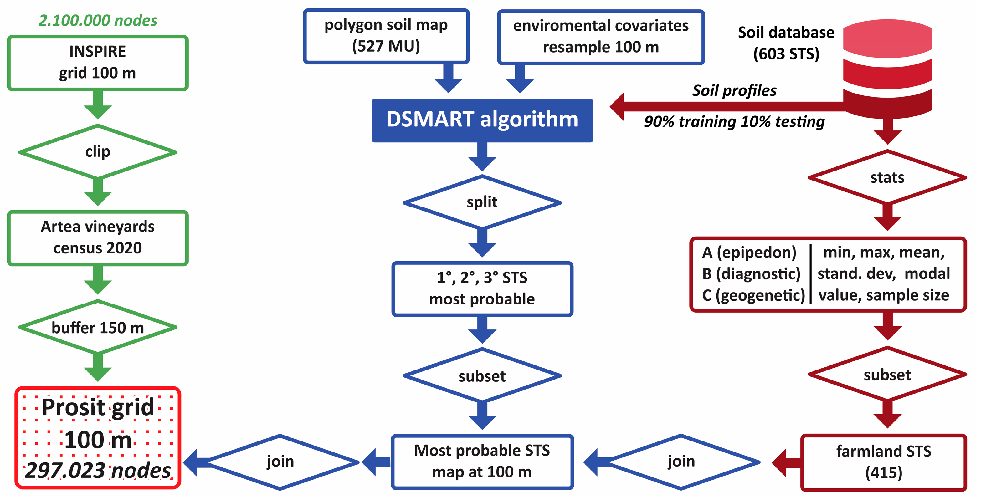
- (1)
- Use soil profile (training set) and intersected covariate values to build a decision tree to predict the spatial distribution of soil classes or STSs.
- (2)
- Extraction of the subset from the soil database corresponding to the land cover class “agriculture” (farmland STS).
- (3)
- For the sake of simplicity, the most probable STS is assigned at each grid cell (see Figure 2 for more details).
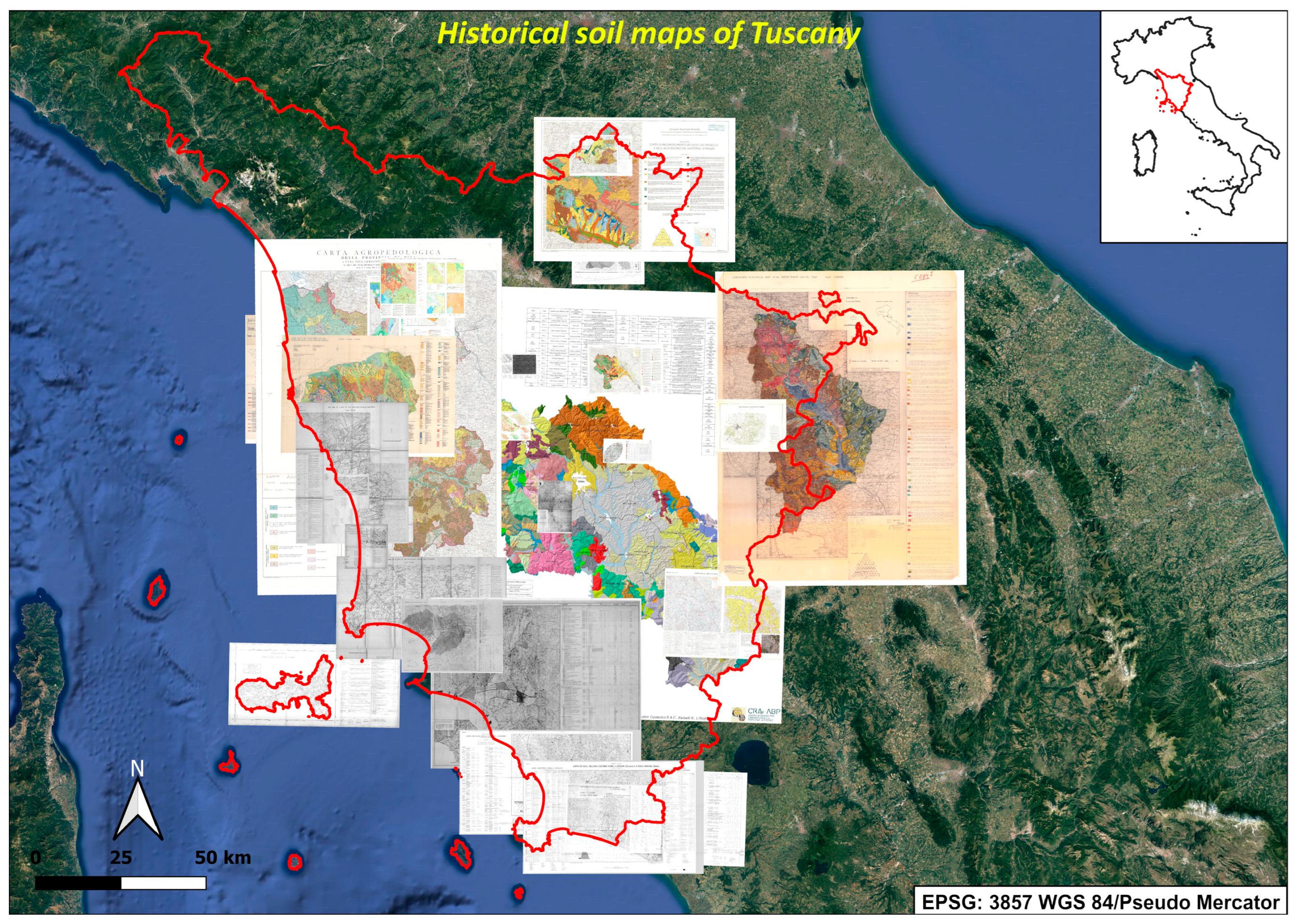
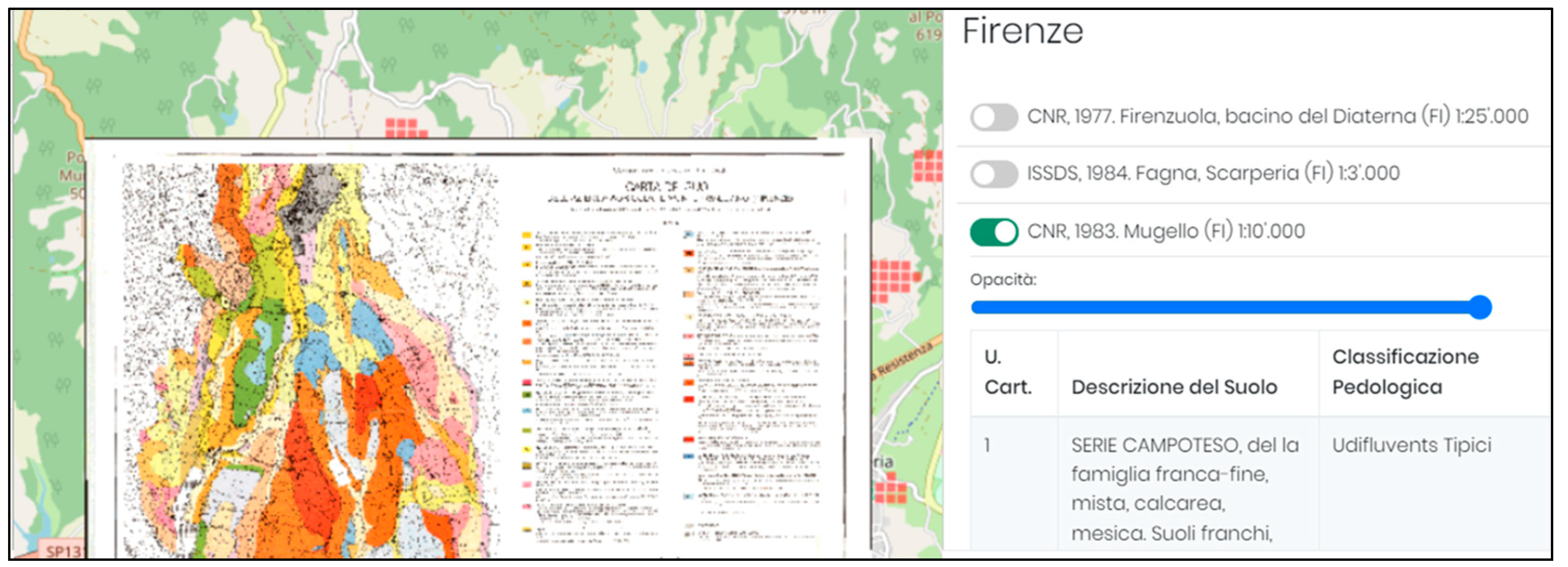
2.3. Digitalization of Existing Paper Maps
2.4. List of Models
2.4.1. New Vineyard Plant Carbon Footprint (by LCA)
2.4.2. Hydrological and Physical Models
Water Stress Risk in the Pre-Planting Phase
Erosion Susceptibility by RUSLE Model and Identification of the Maximum Vine Row Length
Susceptibility to Waterlogging and Surface Runoff: Useful Information to Guide the Hydrological Design of a New Vineyard
2.4.3. Identification of Most Suitable Rootstocks
2.4.4. Soil Chemical–Physical Properties as a Basis for Pre-Planting Fertilization
3. Results and Discussion
3.1. Soil Data Elaboration
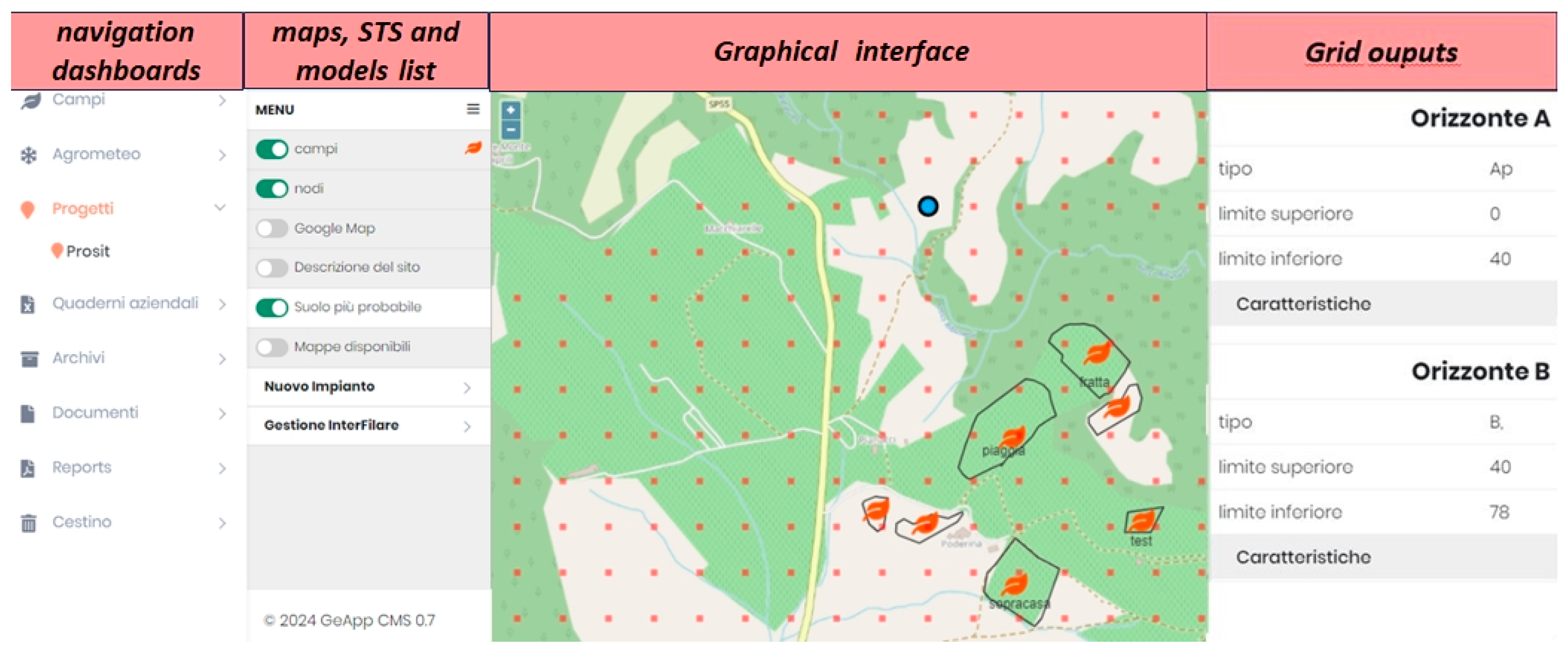
3.2. Graphical User Interface, Digitalized Maps, and WebGis
3.3. Models Results
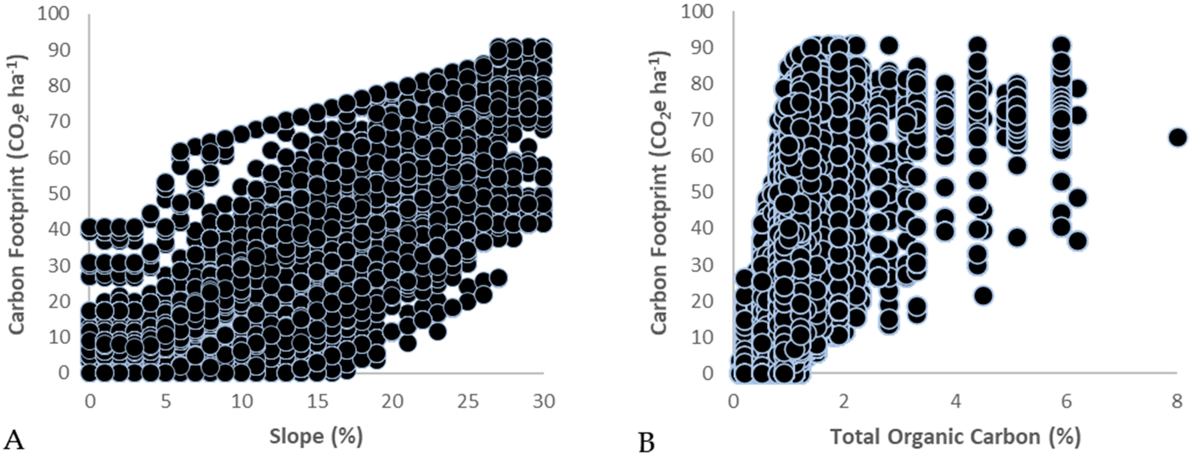
3.3.1. Sustainability Assessment by Carbon Footprint
3.3.2. Hydrological and Physical Model
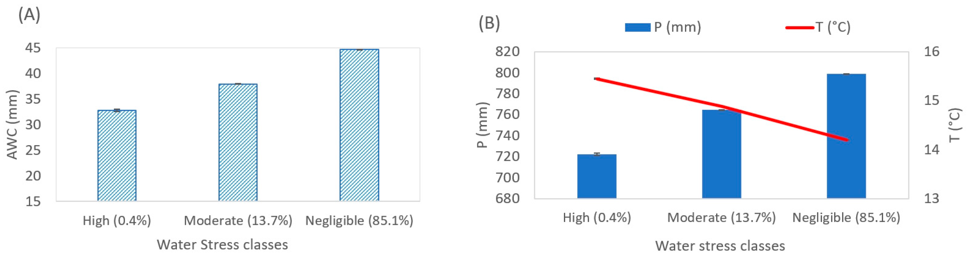
Water Stress Risk
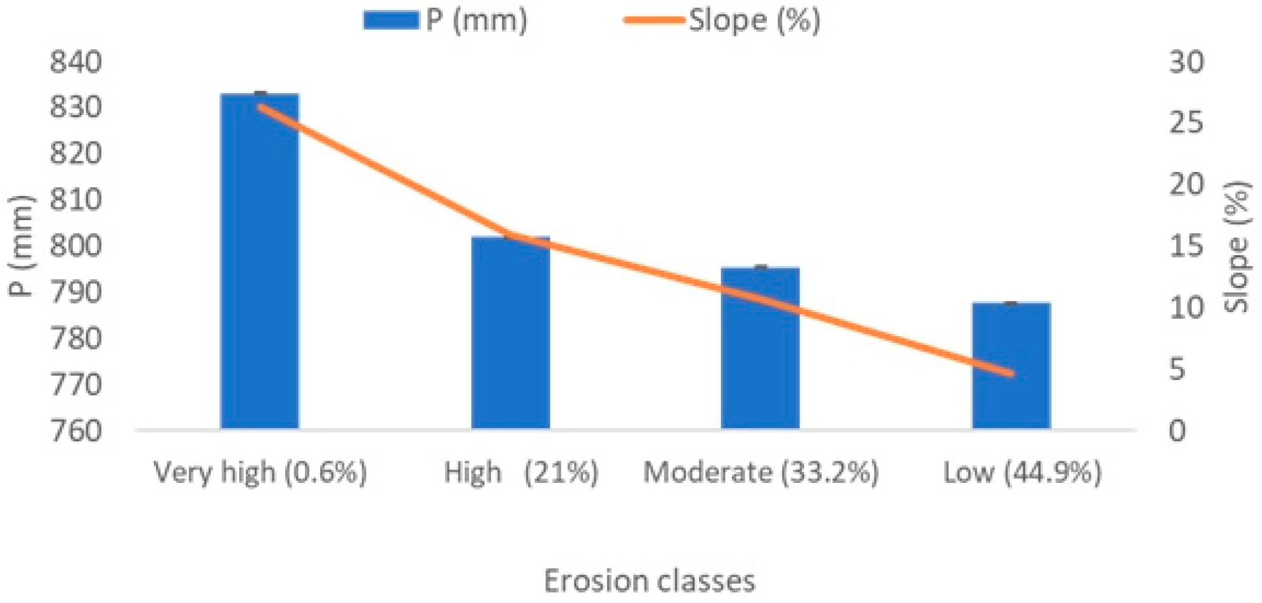
Erosion Risk
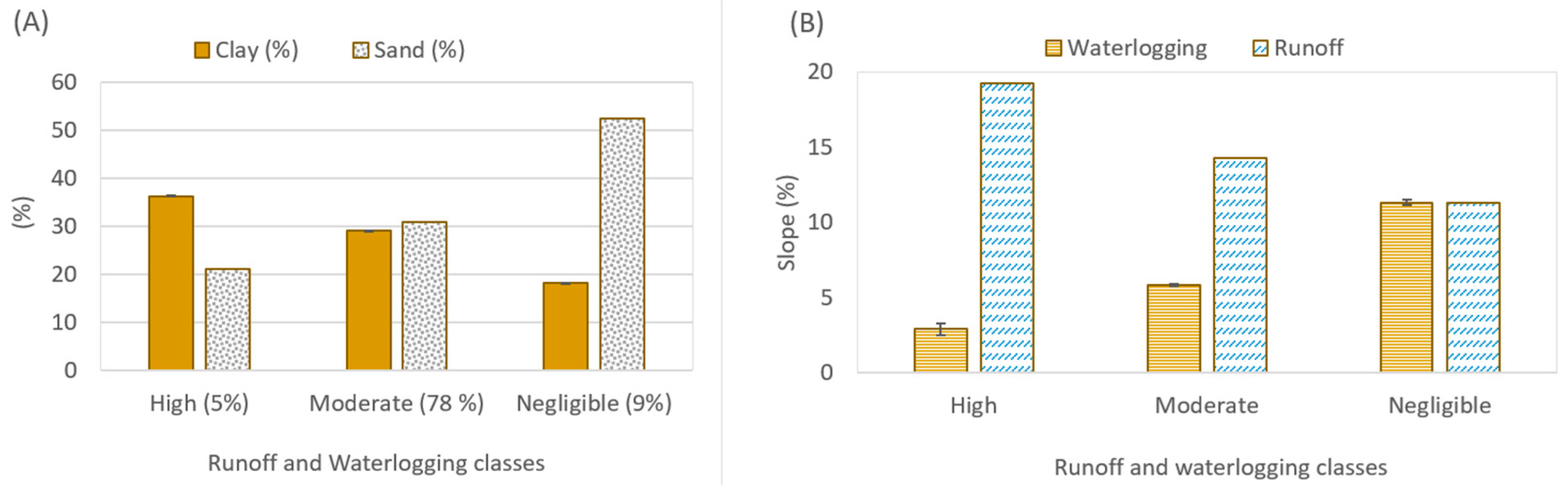
Runoff and Waterlogging Susceptibility
3.3.3. Rootstocks Selection
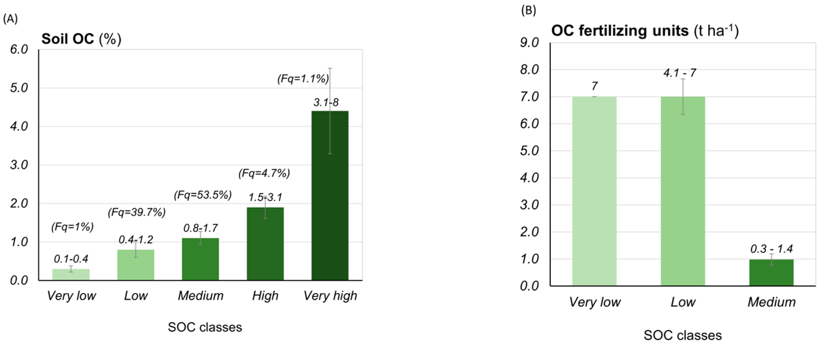
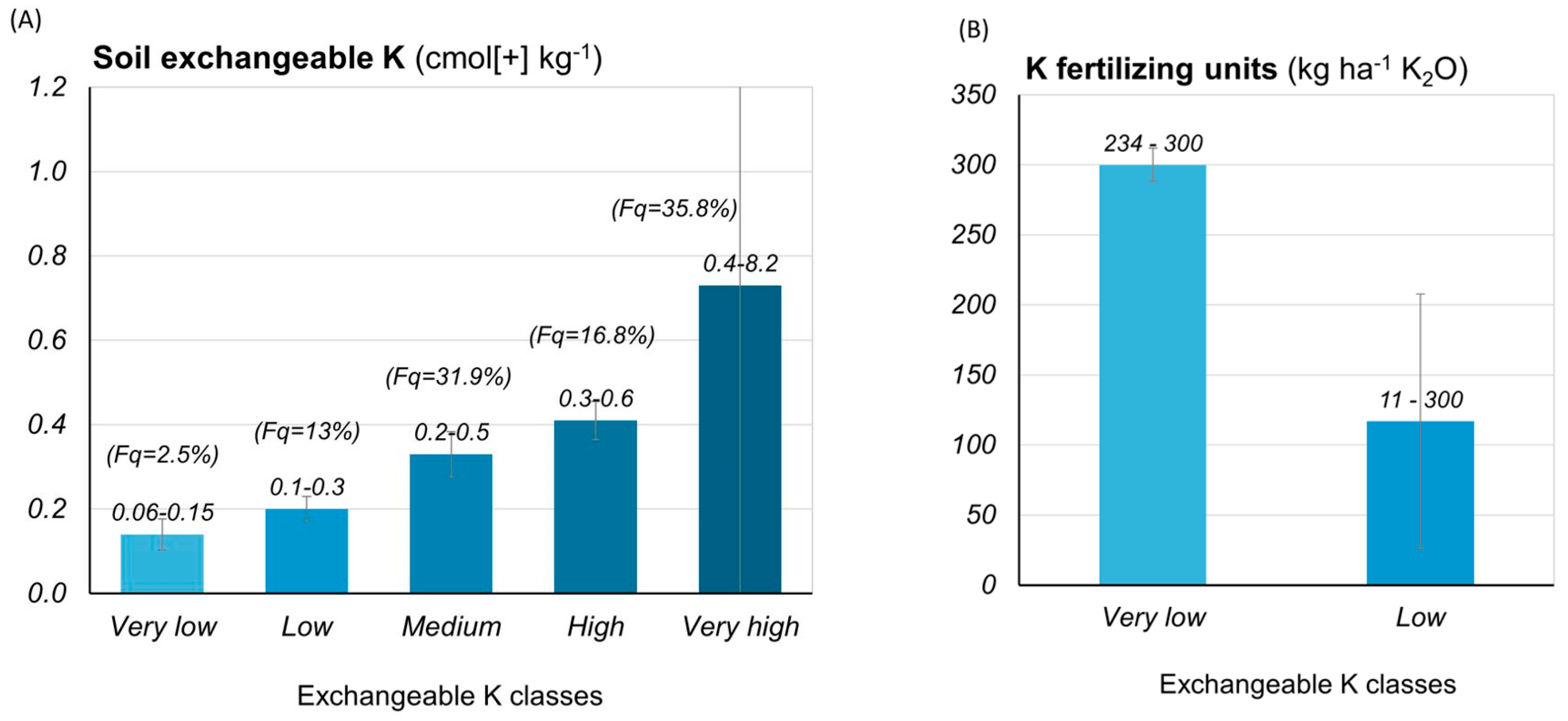
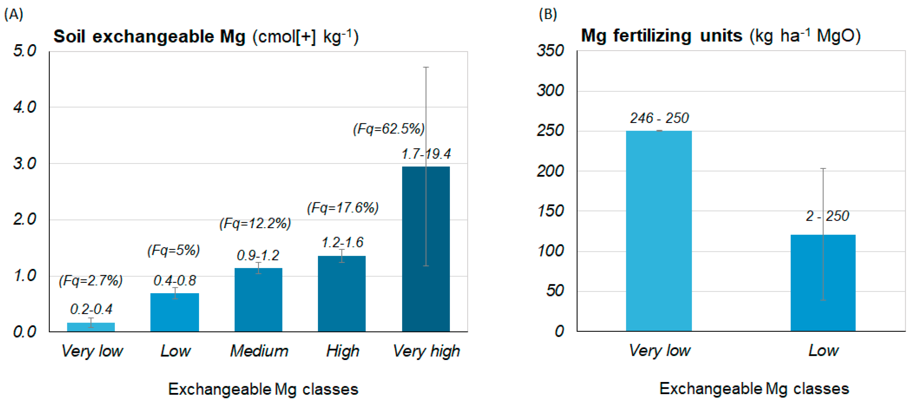
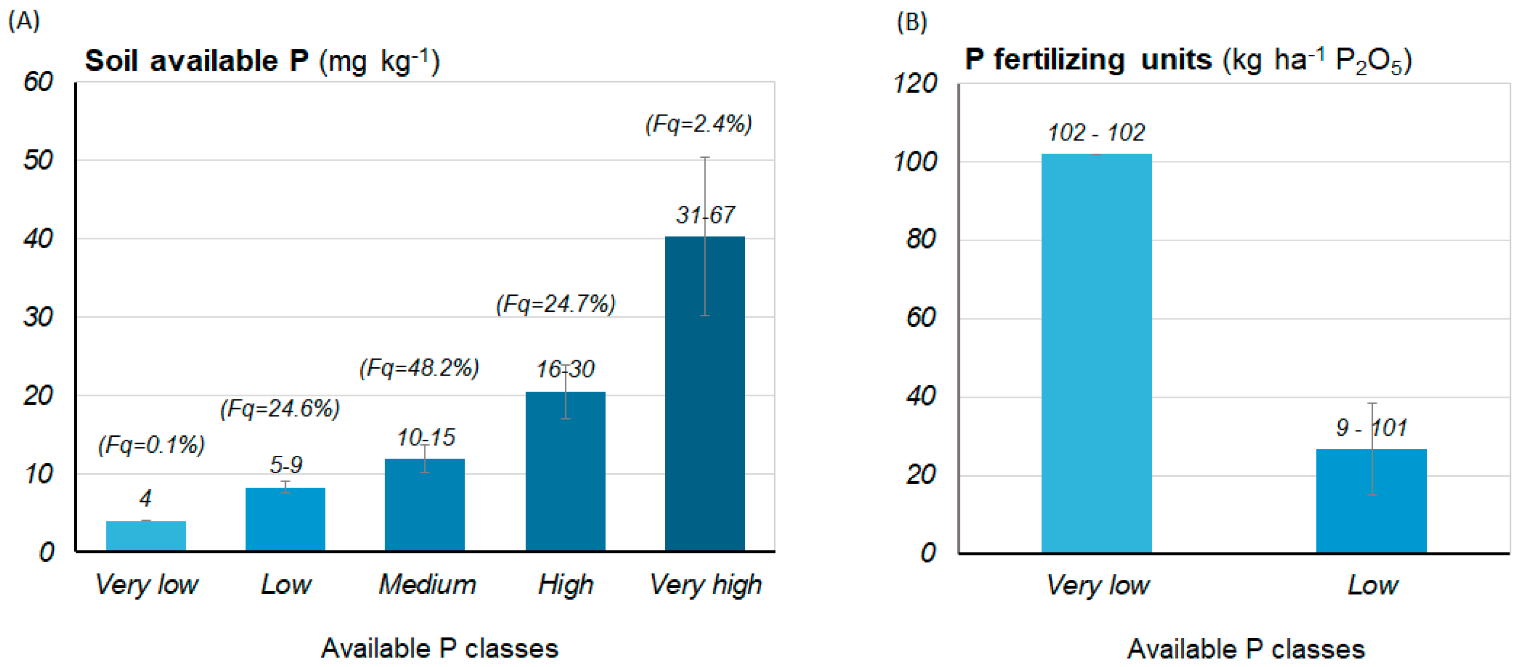
3.3.4. Nutritional Model
4. Conclusions
Author Contributions
Funding
Data Availability Statement
Acknowledgments
Conflicts of Interest
References
- Gil, J.; Alter, E.; La Rota, M.J.; Tello, E.; Galletto, V.; Padró, R.; Marull, J. Towards an agroecological transition in the Mediterranean: A bioeconomic assessment of viticulture farming. J. Clean. Prod. 2022, 380, 134999. [Google Scholar] [CrossRef]
- Cots-Folch, R.; Martínez-Casasnovas, J.A.; Ramos, M. C Land terracing for new vineyard plantations in the north-eastern Spanish Mediterranean region: Landscape effects of the EU Council Regulation policy for vineyards’ restructuring. Agric. Ecosyst. Environ. 2006, 115, 88–96. [Google Scholar] [CrossRef]
- Kosmas, C.; Danalatos, N.; Cammeraat, L.H.; Chabart, M.; Diamantopoulos, J.; Farand, R.; Gutierrez, L.; Jacob, A.; Marques, H.; Martínez-Fernandez, J.; et al. The effect of land use on runoff and soil erosion rates under Mediterranean conditions. Catena 1997, 29, 45–59. [Google Scholar] [CrossRef]
- Cerdan, O.; Govers, G.; Le Bissonnais, Y.; Van Oost, K.; Poesen, J.; Saby, N.; Gobin, A.; Vacca, A.; Quinton, J.; Auerswald, K.; et al. Rates and spatial variations of soil erosion in Europe: A study based on erosion plot data. Geomorphology 2010, 122, 167–177. [Google Scholar] [CrossRef]
- Van Leeuwen, C.; Roby, J.P.; De Rességuier, L. Soil-related terroir factors: A review. OENO ONE 2018, 52, 173–188. [Google Scholar] [CrossRef]
- Pomarici, E.; Corsi, A.; Mazzarino, S.; Sardone, R. The Italian Wine Sector: Evolution, Structure, Competitiveness and Future Challenges of an Enduring Leader. Ital. Econ. J. 2021, 7, 259–295. [Google Scholar] [CrossRef]
- Van Leeuwen, C.; Destrac-Irvine, A.; Dubernet, M.; Duchêne, E.; Gowdy, M.; Marguerit, E.; Pieri, P.; Parker, A.; de Rességuier, L.; Ollat, N. An Update on the Impact of Climate Change in Viticulture and Potential Adaptations. Agronomy 2019, 9, 514. [Google Scholar] [CrossRef]
- Centro Studi Tagliacarne-Unioncamere, Imprese agricole e Cambiamento, 9 June 2023. Available online: https://www.tagliacarne.it/ricerche-20/altri_studi_ed_analisi_economiche-89/ (accessed on 8 August 2023).
- Javaid, M.; Haleem, A.; Singh, R.P.; Suman, R. Enhancing smart farming through the applications of Agriculture 4.0 technologies. Int. J. Intell. Netw. 2022, 3, 150–164. [Google Scholar] [CrossRef]
- GEAPP. La piattaforma integrata per l’agricoltura 4.0. Available online: https://app.geapp.net/utente/registrazione “WebApp Demo” (accessed on 8 March 2024).
- Terribile, F.; Bonfante, A.; D’Antonio, A.; De Mascellis, R.; De Michele, C.; Langella, G.; Basile, A. A geospatial decision support system for supporting quality viticulture at the landscape scale. Comput. Electron. Agric. 2017, 140, 88–102. [Google Scholar] [CrossRef]
- Tardaguila, J.; Stoll, M.; Gutiérrez, S.; Proffitt, T.; Diago, M.P. Smart applications and digital technologies in viticulture: A review. Smart Agric. Technol. 2021, 1, 100005. [Google Scholar] [CrossRef]
- Zhai, Z.; Martínez, J.F.; Beltran, V.; Martínez, N.L. Decision support systems for agriculture 4.0: Survey and challenges. Comput. Electron. Agric. 2020, 170, 1052. [Google Scholar] [CrossRef]
- INSPIRE 2021 (16/03/2021). Available online: https://ec.europa.eu/eurostat/web/gisco/geodata/reference-data/grids (accessed on 8 August 2023).
- A.R.T.E.A Azienda Regionale Toscana per le Erogazioni in Agricoltura. Available online: https://www.artea.toscana.it/ (accessed on 8 August 2023).
- GeoPackage. 2023. Available online: https://www.geopackage.org (accessed on 8 August 2023).
- Agroclima Dati Agroclimatici 1981/2010. Available online: https://www.reterurale.it/agroclima (accessed on 8 August 2023).
- Geoscopio 2023 Regione Toscana. Available online: http://www502.regione.toscana.it/geoscopio/pedologia.html (accessed on 8 August 2023).
- IUSS Working Group WRB. World Reference Base for Soil Resources 2014, Update 2015. In International Soil Classification System for Naming Soils and Creating Legends for Soil Maps; World Soil Resources Reports No. 106; FAO: Rome, Italy, 2015. [Google Scholar]
- Odgers, N.P.; Sun, W.; McBratney, A.B.; Minasny, B.; Clifford, D. Disaggregating and harmonising soil map units through resampled classification trees. Geoderma 2014, 214–215, 91–100. [Google Scholar] [CrossRef]
- McBratney, A.B.; Mendonça Santos, M.L.; Minasny, B. On digital soil mapping. Geoderma 2003, 117, 3–52. [Google Scholar] [CrossRef]
- INSPIRE Thematic Working Group Soil. D2.8.III.3 Data Specification on Soil—Technical Guidelines; European Commission Joint Research Centre: Brussels, Belgium, 2013. [Google Scholar]
- Costantini, E.A.C.; Barbetti, R.; Fantappié, M.; L’Abate, G.; Lorenzetti, R.; Magini, S. Pedodiversity. In The Soils of Italy; World Book Series; Costantini, E.A.C., Dazzi, C., Eds.; Springer Science Business, Media: Dordrecht, The Netherlands, 2013. [Google Scholar]
- Dsmartr-Package: Dsmartr: An R Implementation of the DSMART Algorithm. Available online: https://rdrr.io/github/obrl-soil/dsmartr/man/dsmartr-package.html (accessed on 4 March 2024).
- Wilkinson, M.D.; Dumontier, M.; Aalbersberg, I.J.; Appleton, G.; Axton, M.; Baak, A.; Blomberg, N.; Boiten, J.W.; da Silva Santos, L.B.; Bouwman, J.; et al. The FAIR Guiding Principles for scientific data management and stewardship. Sci. Data 2016, 3, 1–9. [Google Scholar] [CrossRef] [PubMed]
- Menke, K.; Smith, J.; Pirelli, L.; Van Hosen, J. Mastering QGIS; Packt Publishing Ltd.: Birmingham, UK, 2015. [Google Scholar]
- Graser, A.; Peterson, G.N. QGIS Map Design; Sherman, G., Ed.; Locate Press: New York, NY, USA, 2019. [Google Scholar]
- ISO 14044:2006; Environmental management—Life cycle assessment—Requirements and guidelines. ISO: London, UK, 2006.
- Product Environmental Footprint Category Rules (PEFCR) for Still and Sparkling Wine; European Commission: Brussels, Belgium, 26 April 2018.
- IPCC. Climate Change 2014: Synthesis Report. Contribution of Working Groups I, II and III to the Fifth Assessment Report of the Intergovernmental Panel on Climate Change; Core Writing Team, Pachauri, R.K., Meyer, L.A., Eds.; IPCC: Geneva, Switzerland, 2014; 151p. [Google Scholar]
- Costantini, E.A.C.; Agnelli, A.E.; Fabiani, A.; Gagnarli, E.; Mocali, S.; Priori, S.; Simoni, S.; Valboa, G. Short-term recovery of soil physical, chemical, micro-and mesobiological functions in a new vineyard under organic farming. Soil 2015, 1, 443–457. [Google Scholar] [CrossRef]
- Cerdà, A.; Keesstra, S.D.; Rodrigo-Comino, J.; Novara, A.; Pereira, P.; Brevik, E.; Giménez-Morera, A.; Fernández-Raga, M.; Pulido, M.; di Prima, S.; et al. Runoff initiation, soil detachment and connectivity are enhanced as a consequence of vineyards plantations. J. Environ. Manag. 2017, 202, 268–275. [Google Scholar] [CrossRef]
- Refinement to the 2006 IPCC Guidelines for National Greenhouse Gas Inventories; Calvo Buendia, E.; Tanabe, K.; Kranjc, A.; Baasansuren, J.; Fukuda, M.; Ngarize, S.; Osako, A.; Pyrozhenko, Y.; Shermanau, P.; Federici, S. (Eds.) Refinement to the 2006 IPCC Guidelines for National Greenhouse Gas Inventories; IPCC: Genève, Switzerland, 2019. [Google Scholar]
- D’Avino, L.; Di Bene, C.; Farina, R.; Francesco, R. Introduction of Cardoon (Cynara cardunculus L.) in a Rainfed Rotation to Improve Soil Organic Carbon Stock in Marginal Lands. Agronomy 2020, 10, 946. [Google Scholar] [CrossRef]
- Razza, F.; D’Avino, L.; L’Abate, G.; Lazzeri, L. The role of compost in bio-waste management and circular economy. In Designing Sustainable Technologies, Products and Policies—From Science to Innovation; Benetto, E., Gericke, K., Guiton, M., Eds.; Springer Nature International Publishing AG: Berlin/Heidelberg, Germany, 2018; pp. 133–143. ISBN 978-3-319-66980-9. [Google Scholar] [CrossRef]
- Wei, W.; Larrey-Lassalle, P.; Faure, T.; Dumoulin, N.; Roux, P.; Mathias, J.D. How to Conduct a Proper Sensitivity Analysis in Life Cycle Assessment: Taking into Account Correlations within LCI Data and Interactions within the LCA Calculation Model. Environ. Sci. Technol. 2015, 49, 377–385. [Google Scholar] [CrossRef] [PubMed]
- Santos, J.A.; Fraga, H.; Malheiro, A.C.; Moutinho-Pereira, J.; Dinis, L.T.; Correia, C.; Moriondo, M.; Leolini, L.; Dibari, C.; Costafreda-Aumedes, S.; et al. A review of the potential climate change impacts and adaptation options for European viticulture. Appl. Sci. 2020, 10, 3092. [Google Scholar] [CrossRef]
- Deloire, A.; Carbonneau, A.; Wang, Z.; Ojeda, H. Vine and water: A short review. J. Int. Sci. Vigne Vin. 2004, 38, 1–13. [Google Scholar] [CrossRef]
- Mirás-Avalos, J.M.; Araujo, E.S. Optimization of Vineyard Water Management: Challenges, Strategies, and Perspectives. Water 2021, 13, 746. [Google Scholar] [CrossRef]
- Thornthwaite, C.W.; Mather, J.R. Instructions and tables for computing potential evapotranspiration and the water balance. Climatology 1957, 10, 181–311. [Google Scholar]
- Gaiotti, F. Gestione dell’irrigazione per la qualità in vigneto. L’uso corretto della microirrigazione; CREA-VIT Conegliano: Albinea, Italy, 2012. [Google Scholar]
- Armiraglio, S.; Cerabolini, B.; Gandellini, F.; Gandini, P.; Andreis, C. Calcolo informatizzato del bilancio idrico del suolo. “Natura Bresciana”. Ann. Mus. Civ. Sc. Nat. Brescia 2003, 33, 209–216. [Google Scholar]
- Saxton, K.E.; Rawls, W.J. Soil water characteristic estimates by texture and organic matter for hydrologic solutions. Soil Sci. Soc. Am. J. 2006, 70, 1569–1578. [Google Scholar] [CrossRef]
- Knijff, J.; Jones, R.; Montanarella, L. Soil Erosion Risk Assessment in Italy; European Soil Bureau: Ispra, Italy, 2002. [Google Scholar]
- Renard, K.G.; Foster, G.R.; Weesies, G.A.; McCool, D.K.; Yoder, D.C. Predicting soil erosion by water: A guide to conservation planning with the Revised Universal Soil Loss Equation (RUSLE). In USDA Agriculture Handbook; USDA: Washington, DC, USA, 1997; 404p. [Google Scholar]
- Diodato, N.; Bellocchi, G. Assessing and modelling changes in rainfall erosivity at different climate scales. Earth Surf. Process. Landf. 2009, 34, 969–980. [Google Scholar] [CrossRef]
- Napoli, M.; Cecchi, S.; Orlandini, S.; Mugnai, G.; Zanchi, C.A. Simulation of field-measured soil loss in Mediterranean hilly areas (Chianti, Italy) with RUSLE. Catena 2016, 145, 246–256. [Google Scholar] [CrossRef]
- Bazzoffi, P.; Francaviglia, R.; Neri, U.; Napoli, R.; Marchetti, A.; Falcucci, M.; Pennelli, B.; Simonetti, G.; Barchetti, A.; Migliore, M.; et al. Environmental effectiveness of GAEC cross-compliance Standard 1.1a (temporary ditches) and 1.2g(permanent grass cover of set-aside) in reducing soil erosion and economic evaluation of the competitiveness gap for farmers. Ital. J. Agron. 2016, 10, 9. [Google Scholar] [CrossRef]
- Soil Conservation Service (SCS). National Engineering Handbook, Section 4: Hydrology; Department of Agriculture: Washington, DC, USA, 1972; 762p. [Google Scholar]
- Rahemi, A.; Dodson Peterson, J.C.; Lund, K.T. Choosing Grape Rootstock. In Grape Rootstocks and Related Species; Springer: Cham, Switzerland, 2022. [Google Scholar] [CrossRef]
- Lambert, J.; Anderson, M.; Wolpert, J. Vineyard nutrient needs vary with rootstocks and soils. Calif. Agr. 2008, 62, 202–207. [Google Scholar] [CrossRef]
- Bihari, Z.; Tóth, J.P.; Zsigrai, G.; Balling, P.; Fischinger, R.; Éles, S. Rootstock effects on vegetative growth of ‘Furmint’. Acta Hortic. 2016, 1136, 39–44. [Google Scholar] [CrossRef]
- Goldammer, T. Grape Grower’s Handbook. A Guide to Viticulture for Wine Production; Apex Publishers: Centreville, Virginia, 2012. [Google Scholar]
- Costantini, E.A.C. (Ed.) Metodi di Valutazione dei Suoli e Delle Terre; Cantagalli: Siena, Italy, 2006. [Google Scholar]
- Rootstock Comparison Chart. Available online: https://www.vivairauscedo.com/indice-prodotti/portinnesti/#!/descrizione_portinnesti (accessed on 18 February 2024).
- Fregoni, M. Viticoltura di Qualità, Trattato Dell’eccellenza da Terroir, 3rd ed.; Tecniche Nuove editore: Milan, Italy, 2013. [Google Scholar]
- LGNTA—Linee Guida Nazionali di Produzione Integrata—Tecniche Agronomiche. Ministero Delle Politiche Agricole, Alimentari e Forestali, Direzione Generale Dello Sviluppo Rurale, Organismo Tecnico Scientifico, Rev. 6. 2022. Available online: https://www.reterurale.it/flex/cm/pages/ServeBLOB.php/L/IT/IDPagina/24284 (accessed on 4 March 2024).
- Masoni, A.; Bechini, L.; Fagnano, M.; Marino Gallina, P. Interventi sulle caratteristiche chimiche e biologiche del suolo: Fertilizzazione. In Agronomia; Ceccon, P., Fagnano, M., Grignani, C., Monti, M., Orlandini, S., Eds.; Edises-SIA: Napoli, Italy, 2017; Volume 9, pp. 279–323. [Google Scholar]
- Regione Campania—Assessorato Agricoltura. Disciplinare di Produzione Integrata. Norme Tecniche Generali. Allegato A. 2020. Available online: http://www.agricoltura.regione.campania.it/disciplinari/DRD_46-01-04-22.pdf (accessed on 4 March 2024).
- Regione Emilia-Romagna—Direzione Generale Agricoltura, Caccia e Pesca 2020. Disciplinare di Produzione Integrata—Norme Generali, Edizione 2020. Available online: https://agricoltura.regione.emilia-romagna.it/produzioni-agroalimentari/temi/bio-agro-climambiente/agricoltura-integrata/disciplinari-produzione-integrata-vegetale/Collezione-dpi/dpi_2020/copy2_of_norme_generali-2020-def.pdf/@@download/file/Norme_generali%202020%20def.pdf (accessed on 4 March 2024).
- Soil Survey Staff. Keys to Soil Taxonomy, 13th ed.; USDA-Natural Resources Conservation Service: Washington, DC, USA, 2022. [Google Scholar]
- Rossiter, D.G.; Zeng, R.; Zhang, G.L. Accounting for taxonomic distance in accuracy assessment of soil class predictions. Geoderma 2017, 292, 118–127. [Google Scholar] [CrossRef]
- Costantini, E.A.C.; Priori, S. Avoiding improper earth movements before planting tree crops. In FAO and ITPS. Recarbonizing Global Soils: A Technical Manual of Recommended Management Practices; Volume 3: Cropland, Grassland, Integrated Systems and Farming Approaches—Practices Overview; FAO: Rome, Italy, 2021. [Google Scholar] [CrossRef]
- Cruz-Ruiz, E.; Cristòfol, F.J.; Zamarreño-Aramendia, G. Managing Digital Presence in Wineries Practicing Heroic Agriculture: The Cases of Ribeira Sacra and Lanzarote (Spain). Agronomy 2023, 13, 946. [Google Scholar] [CrossRef]
- FAO; ITPS. Recarbonizing Global Soils—A Technical Manual of Recommended Management Practices; Volume 1: Introduction and Methodology; FAO: Rome, Italy, 2021. [Google Scholar] [CrossRef]


| Soil Water Potential (MPa) | Vine Water Stress Tolerance (MPa) | |
|---|---|---|
| August–October 0.2–0.4 | April–July; November <0.2 | |
| >0.6 | VH | VH |
| 0.6–0.4 | H | VH |
| 0.4–0.2 | M | H |
| <0.2 | N | N |
| Site Slope (%) | RC Class | ||
|---|---|---|---|
| High | Moderate | Negligible | |
| <5 | H(S) | M(S) | M(S) |
| 5–10 | M(S) | M(S) | N |
| 10–20 | M(R) | M(S) | N |
| 20–35 | H(R) | M(S) | N |
| 35–45 | H(R) | H(R) | M(R) |
| >45 | H(R) | H(R) | H(R) |
| Parameter Input Models Data | ||||||
|---|---|---|---|---|---|---|
| Site | Min | Q1 | Me./Mo. | Q3 | Max | Unit Measure |
| elevation | 0 | 103 | 229 | 307 | 1019 | m. a.s.l. |
| aspect | 5 | 145 | 191 | 233 | 350 | ° |
| slope | 0 | 5 | 9 | 12 | 68 | % |
| Climate | ||||||
| air temperature | 10.3 | 13.3 | 13.8 | 14.3 | 15.7 | °C |
| precipitation | 625 | 781 | 790 | 813 | 1028 | mm |
| Soil quality | ||||||
| rooting depth | 20 | 89 | 110 | 132 | 250 | cm |
| root impediment | paralithic contact | class | ||||
| intern. drainage | well drained | 7 ordinal level | ||||
| Soil layer (0–30 cm) | ||||||
| available P | 4 | 10 | 12 | 16 | 77 | mg/kg |
| bulk density | 0.33 | 1.39 | 1.46 | 1.5 | 1.86 | g/cm3 |
| field capacity | 19.6 | 66.1 | 75.3 | 96.1 | 147 | mm |
| wilting point | 11.1 | 33.5 | 38.8 | 50.4 | 103 | mm |
| coarse fragments | 0 | 1.5 | 6 | 18.5 | 73 | g/100 g |
| org. carbon | 0.1 | 0.9 | 1.1 | 1.3 | 7 | g/100 g |
| tot. nitrogen | 0.2 | 0.7 | 1 | 1.3 | 8.0 | g/kg |
| Soil-derived profile, from surface to bedrock, 1 to 4 master horizons (A, B, C, R) | ||||||
| horizon type | B | class (A, B, C, R) | ||||
| upper limit | 0 | 0 | 34 | 54 | 106 | cm |
| lower limit | 2 | 40 | 72 | 101 | 250 | cm |
| coarse fragments | 0 | 0 | 6 | 24 | 90 | g/100 g |
| clay | 0 | 19 | 27 | 38 | 80 | g/100 g |
| silt | 1 | 31 | 38 | 45 | 92 | g/100 g |
| sand | 1 | 18.8 | 32 | 48 | 98 | g/100 g |
| tot. carbonates | 0 | 0 | 7 | 15 | 84 | g/100 g |
| org. carbon | 0.06 | 0.48 | 0.77 | 1.13 | 7.0 | g/100 g |
| tot. nitrogen | 0.00 | 0.46 | 0.79 | 1.15 | 8 | g/kg |
| reaction | 4.2 | 7.1 | 7.7 | 8 | 8.7 | pH H2O |
| exchang. Ca2+ | 0.2 | 10.5 | 14.9 | 19.7 | 97 | meq/100 g |
| exchang. Mg+ | 0.08 | 1.32 | 2.29 | 3.49 | 27 | meq/100 g |
| exchang. K+ | 0 | 0.23 | 0.31 | 0.45 | 23 | meq/100 g |
| ESP | 0 | 0.9 | 1.9 | 3.3 | 83 | meq/100 g |
| CEC | 0.7 | 14.9 | 19.8 | 24.5 | 60 | meq/100 g |
| electr. conduct. | 0.01 | 0.12 | 0.16 | 0.26 | 7.6 | (1:2.5) dS/m |
| Models’ Outputs | ||||||
|---|---|---|---|---|---|---|
| Eco-Sustainability | Min | Q1 | Me./Mo | Q3 | Max | Unit Measure |
| carbon footprint | 0 | 5.6 | 15.1 | 28.5 | 91.0 | t CO2e/ha |
| Water stress | ||||||
| cuttings water stress | Negligible | 4 classes | ||||
| Hydrological and physical models | ||||||
| erosion susceptibility | Low susceptibility | 4 classes | ||||
| soil loss | 0.1 | 6.2 | 12.3 | 18.8 | 115 | t/ha |
| max. length of rows | 50 | 100 | 100 | 100 | 100 | m |
| Water limitations | ||||||
| runoff risk | Medium risk | 3 classes | ||||
| waterlogging risk | Stagnation moderate | 3 classes | ||||
| Rootstock | ||||||
| suitable rootstock | M1–M3–M4–41B–420A–Gravesac–Fercal | 15 rootstocks (42 clusters) | ||||
| Soil OC and nutrient requirement for basal fertilization | ||||||
| Potassium (K2O) | 0 | 0 | 0 | 0 | 300 | kg/ha |
| Phosphorus (P2O5) | 0 | 0 | 0 | 0 | 102 | kg/ha |
| Magnesium (MgO) | 0 | 0 | 0 | 0 | 250 | kg/ha |
| Organic C | 0 | 0.92 | 1.10 | 7 | 7 | t/ha |
| Water Stress Class | Tuscan Provinces | Total | |||||||||
|---|---|---|---|---|---|---|---|---|---|---|---|
| AR | FI | GR | LI | LU | MS | PI | PO | PT | SI | ||
| High | 0.00 | 0.01 | 0.38 | 0.02 | 0.00 | 0.00 | 0.00 | 0.00 | 0.00 | 0.01 | 0.43 |
| Moderate | 1.15 | 1.49 | 7.11 | 0.64 | 0.06 | 0.01 | 0.48 | 0.03 | 0.08 | 2.76 | 13.82 |
| Negligible | 12.69 | 23.49 | 9.48 | 4.13 | 2.05 | 1.09 | 6.46 | 0.75 | 1.69 | 23.93 | 85.75 |
| Total | 13.84 | 25.00 | 16.96 | 4.79 | 2.11 | 1.10 | 6.94 | 0.78 | 1.77 | 26.70 | 100.00 |
| Group * | n. | Area % | Fertility Class | Total CaCO3 Class | Salinity Class | pH Class |
|---|---|---|---|---|---|---|
| A | 8 | 59.9 | High | <Very calcareous | Low | Neutral/ Alkaline |
| B | 7 | 13.6 | High | <Very calcareous | Medium | Alkaline |
| C | 12 | 6.5 | Medium | Strongly calcareous | Low | Alkaline |
| D | 4 | 5.9 | High | Non-calcareous | Low | Acidic |
| E | 15 | 4.9 | Medium | <Very calcareous | Low | Neutral/ Alkaline |
| F | 14 | 3.3 | Medium | Moderate–Very calcareous | Medium | Alkaline |
| G | 11 | 2.2 | Low | <Moderately calcareous | Low | Neutral |
| H | 10 | 1.3 | Medium | Non-calcareous | Low | Acidic |
| I | 7 | 1.2 | Medium | Very calcareous | High | Alkaline |
Disclaimer/Publisher’s Note: The statements, opinions and data contained in all publications are solely those of the individual author(s) and contributor(s) and not of MDPI and/or the editor(s). MDPI and/or the editor(s) disclaim responsibility for any injury to people or property resulting from any ideas, methods, instructions or products referred to in the content. |
© 2024 by the authors. Licensee MDPI, Basel, Switzerland. This article is an open access article distributed under the terms and conditions of the Creative Commons Attribution (CC BY) license (https://creativecommons.org/licenses/by/4.0/).
Share and Cite
Barbetti, R.; Criscuoli, I.; Valboa, G.; Vignozzi, N.; Pellegrini, S.; Andrenelli, M.C.; L’Abate, G.; Fantappiè, M.; Orlandini, A.; Lachi, A.; et al. A Regional 100 m Soil Grid-Based Geographic Decision Support System to Support the Planning of New Sustainable Vineyards. Agronomy 2024, 14, 596. https://doi.org/10.3390/agronomy14030596
Barbetti R, Criscuoli I, Valboa G, Vignozzi N, Pellegrini S, Andrenelli MC, L’Abate G, Fantappiè M, Orlandini A, Lachi A, et al. A Regional 100 m Soil Grid-Based Geographic Decision Support System to Support the Planning of New Sustainable Vineyards. Agronomy. 2024; 14(3):596. https://doi.org/10.3390/agronomy14030596
Chicago/Turabian StyleBarbetti, Roberto, Irene Criscuoli, Giuseppe Valboa, Nadia Vignozzi, Sergio Pellegrini, Maria Costanza Andrenelli, Giovanni L’Abate, Maria Fantappiè, Alessandro Orlandini, Andrea Lachi, and et al. 2024. "A Regional 100 m Soil Grid-Based Geographic Decision Support System to Support the Planning of New Sustainable Vineyards" Agronomy 14, no. 3: 596. https://doi.org/10.3390/agronomy14030596