
Construction and Validation of Peanut Leaf Spot Disease Prediction Model Based on Long Time Series Data and Deep Learning


1
National Engineering Research Center for Peanut, Shandong Peanut Research Institute, Qingdao 266100, China
2
Research Center of Information Technology, Beijing Academy of Agriculture and Forestry Sciences/National Engineering Research Center for Information Technology in Agriculture/National Engineering Laboratory for Agri-Product Quality Traceability/Meteorological Service Center for Urban Agriculture, China Meteorological Administration-Ministry of Agriculture and Rural Affairs, Beijing 100097, China
3
International PhD School, University of Almería, 04120 Almería, Spain
4
Key Laboratory of Special Fruits and Vegetables Cultivation Physiology and Germplasm Resources Utilization of Xinjiang Production and Construction Crops, College of Agriculture, Shihezi University, Shihezi 832003, China
*
Authors to whom correspondence should be addressed.
Agronomy 2024, 14(2), 294; https://doi.org/10.3390/agronomy14020294
Submission received: 29 December 2023
/
Revised: 18 January 2024
/
Accepted: 25 January 2024
/
Published: 29 January 2024
(This article belongs to the Section Farming Sustainability)
Abstract
:Peanut leaf spot is a worldwide disease whose prevalence poses a major threat to peanut yield and quality, and accurate prediction models are urgently needed for timely disease management. In this study, we proposed a novel peanut leaf spot prediction method based on an improved long short-term memory (LSTM) model and multi-year meteorological data combined with disease survey records. Our method employed a combination of convolutional neural networks (CNNs) and LSTMs to capture spatial–temporal patterns from the data and improve the model’s ability to recognize dynamic features of the disease. In addition, we introduced a Squeeze-and-Excitation (SE) Network attention mechanism module to enhance model performance by focusing on key features. Through several hyper-parameter optimization adjustments, we identified a peanut leaf spot disease condition index prediction model with a learning rate of 0.001, a number of cycles (Epoch) of 800, and an optimizer of Adma. The results showed that the integrated model demonstrated excellent prediction ability, obtaining an RMSE of 0.063 and an of 0.951, which reduced the RMSE by 0.253 and 0.204, and raised the by 0.155 and 0.122, respectively, compared to the single CNN and LSTM. Predicting the occurrence and severity of peanut leaf spot disease based on the meteorological conditions and neural networks is feasible and valuable to help growers make accurate management decisions and reduce disease impacts through optimal fungicide application timing.
1. Introduction
Peanut, a significant cash crop, plays a vital role in global food security. Its yield and quality are crucial, yet they are threatened by peanut leaf spot disease. This widespread affliction, causing necrosis in peanut leaves and stalks, poses a substantial risk to the global peanut industry. Accurately predicting the onset and severity of this disease is essential for implementing effective control strategies and mitigating crop loss [1,2].
Traditionally, the prediction of plant disease incidence and severity has predominantly utilized statistical methods and crop growth models [3,4,5]. However, these conventional monitoring techniques are constrained by temporal and spatial limitations [6,7]. They struggled with complex spatio-temporal data and multi-source information integration, hindering their applicability in precision agriculture. Recently, the burgeoning field of artificial intelligence, especially data-driven and deep learning methods, has garnered attention for its potential in agricultural applications, particularly in plant disease forecasting [8,9,10].
Several studies have illustrated the advance in this research direction. Azadbakht et al. [11] employed machine learning techniques, including Gaussian process regression, Random Forest regression, v-support vector regression, and boosted regression trees, to predict the severity of wheat leaf rust. Guan et al. [12] utilized K-Nearest Neighbor (KNN), Support Vector Machines (SVMs), and Back-Propagation (BP) neural network classifiers to assess Hyperspectral feature wavelengths of peanut leaf spot disease, predicting its severity. Bhatia et al. [13] explored the use of random forest approaches to analyze soil microbial communities, predicting the likelihood of blight occurrence. Xiao et al. [14] treated cotton pest and disease incidence as a time-series classification problem, and addressed it with LSTM networks, demonstrating its superiority over other machine learning methods such as KNN, Support Vector Classification (SVC), and Random Forest (RF) in predicting cotton bollworm incidence.
The prevalence of plant diseases was intricately linked to weather conditions and pathogen transmission [15,16,17]. Seasonal plant diseases, in particular, were influenced by varying climatic and environmental variables [18]. Our understanding and forecasting capabilities using mathematical or statistical techniques remain inherently limited [19]; fortunately, deep learning methods can analyze these data to discern patterns between climatic conditions and plant diseases, enabling future outbreak predictions. The Aprioro algorithm has been used to determine associations between meteorological factors and cotton pests and diseases, subsequently developing a time-series prediction model using LSTM [20]. Fenu and Malloci [21] investigated the use of meteorological variables from regional weather stations to predict potato late blight, and concluded that temperature, humidity, and wind speed were critical predictive factors [22]. Similarly, Kim et al. [23] applied LSTM to historical data on rice blast incidence and climatic conditions to predict the rice blast incidence index. Liu et al. [24] used LSTM to study the potential association between environmental factors and plant diseases to establish a prediction model for cucumber downy mildew, which was migrated to be applied to an early warning system for chili pepper pest and disease epidemics in a follow-up study [25]. Huang et al. [26] combined mobile Internet and high-resolution spatio-temporal meteorological data to provide new ideas for pest and disease prediction, and they utilized a machine learning approach to establish a prediction model of Alternaria Leaf Spot disease of apple.
Nowadays, machine learning and artificial intelligence techniques are adapted to uncover complex models and relationships compared to conventional mathematical methods. Particularly, Recurrent Neural Networks (RNN) and LSTM have shown exceptional capability in identifying patterns and trends in time-series data [27,28]. Although the above studies have improved the accuracy of disease prediction to a certain extent, there were still some problems, such as insufficient model generalization ability and limited ability to process the fusion of multi-source data. Commonly, models have used a limited set of variables—temperature, relative humidity, rainfall, and wind speed—potentially overlooking crucial disease-related features. Predominantly, previous studies have employed BP neural networks and generalized regression neural networks (GRNN), which were prone to issues like gradient vanishing or explosion, and struggled with long-term dependencies due to their lack of gating mechanisms [29,30].
To address these challenges, this study has developed a predictive model for peanut leaf spot disease, which leveraged an enhanced CNN-LSTM network, incorporating several years of meteorological data, supplemented by disease field survey data. This approach has culminated in the establishment of a predictive model for peanut leaf spot disease, which was substantiated through two years of continuous experimental validation.
2. Materials and Methods
2.1. Data Acquisition and Normalization
In this study, we used peanut leaf spot disease as the research object and meteorological data as the main data source. The meteorological data were obtained from the open-source meteorological website. Open-Meteo is an open-source weather API and offers free access for non-commercial use (https://open-meteo.com/, accessed on 12 October 2023). We purchased from this website five consecutive years of meteorological data from 2017 to 2023 for the peanut planting base in Laixi, Qingdao City, Shandong Province, containing nine elements, including temperature, humidity, dew point, precipitation, sea level barometric pressure, surface barometric pressure, wind direction, wind speed, and solar radiation. Open-Meteo provides high-resolution open data from 1 to 11 km, which is more reflective of the meteorological conditions over a large area. The monitoring range of a single weather station is very limited, which may be only a few tens of meters, so we calibrate the data through a small weather station at the experimental base. We set the local meteorological data as the dependent variable (Y) and the Open-Meteo data as the independent variable (X). Since both the response and predictor variables contained measurement errors, we performed the calibration process using a linear regression model, Deming, with the goal of minimizing the orthogonal (vertical) distance from the data points to the fitted line, while ensuring that the data timestamps are consistent. It was verified that the RMSE for the temperature of X (Open-Meteo data) versus Y (local small weather station data) was only 0.214.
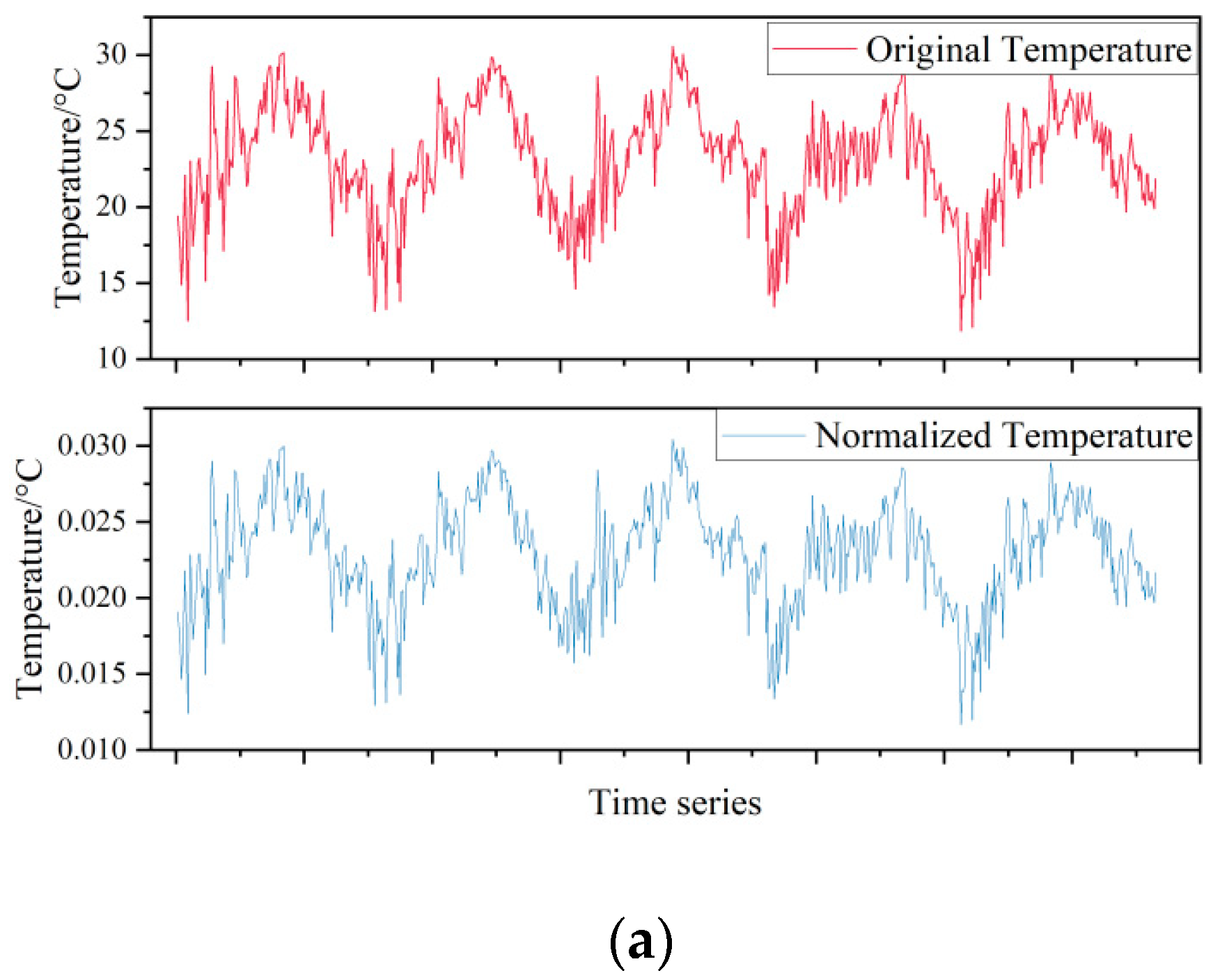
In this study, we used the data from 2017 to 2021 as inputs to the model, and the data from 2022 and 2023 to conduct the actual validation of the model. Considering that if an input has a large scale, its weight update may be larger than other inputs, which may cause the model to rely too much on certain features during training. In order to eliminate the presence of scale effects between different metrics, the data are normalized. Normalization speeds up the convergence of the model while preventing numerical overflow and gradient explosion, and improves the accuracy of the prediction model to some extent. We use the mapminmax function to carry out the normalization operation of the data, and its calculation principle is:
The time series raw meteorological data and normalized data are shown in Figure 1.
2.2. Disease Survey
We studied the relationship between meteorological conditions and peanut leaf spot disease, and in addition to obtaining meteorological data, we needed to investigate the occurrence of peanut leaf spot disease. Peanut plants were cultivated in an experimental field at the Shandong Peanut Research Institute (SPRI) in Laixi City, Qingdao, China, which is located at latitude 36°48′46″ N-longitude 120°30′5″ E. The field is planted biennially in a peanut/wheat/corn rotation. Peanuts are sown in early May each year, and the experimental site is a multi-year peanut cropping field with severe peanut leaf spots (brown spot and black spot). Peanut planting plots were arranged in randomized groups, repeated twice, and the density of peanut planting was 10,000 holes per mu, with two grains per hole. Peanut varieties are “HuaYu”, “LuoHua”, and “PuHua” three series, which are moderate or highly susceptible to leaf spot disease. We use a manual survey method to record the disease index and relative resistance index sampling, from early July to the beginning of September each year for the survey. The severity of peanut leaf spot was assessed on a scale of 0–4, with 0 representing no disease and 4 representing plant death. The leaf spot scoring system was imported and revised from reference [31], and shown in Table 1.
We randomly selected 20 plants in each plot to assess the severity of leaf spot disease. The average disease index (DI) was calculated using the following formula:
Due to the weather anomaly in 2017, peanut disease occurrence was generally light in June and July due to persistent high temperatures and drought, and the rest of the year did not experience weather anomalies. Based on manual surveys, peanut brown spot disease appeared in mid-July, peanut black spot disease appeared in mid-to-late August, and with increased rainfall in mid-to-late August, peanut black spot and brown spot disease occurred in large quantities, and net blotch disease basically did not occur.
2.3. Model Building
2.3.1. Feature Processing Module
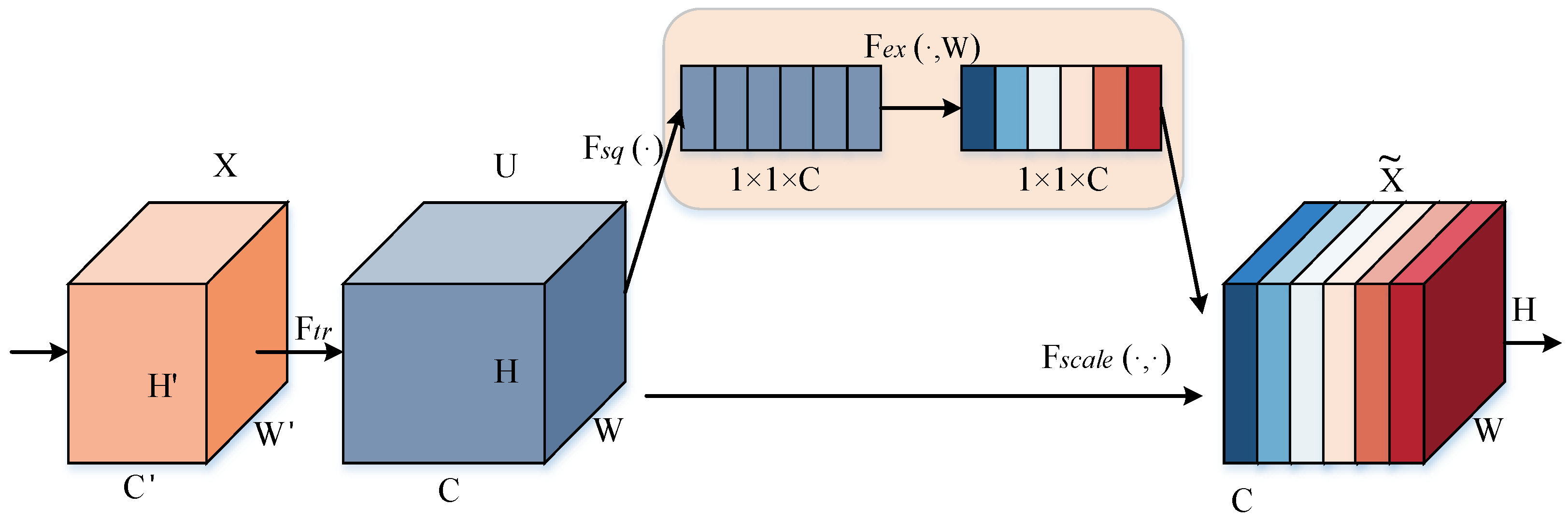
To enable the model to focus on more useful data features, we embedded the SE networks in the network [32]. The traditional feature transfer method is to pass the weights such as the Feature Map of the network to the next layer, while the SE Network Block attention mechanism adaptively recorrects the intensity of the feature response between channels through the global loss function of the network; which is to say, the SE block extracts effective features by augmenting or aligning the corresponding channels for different tasks through the weights of the importance of each feature channel [33]. As shown in Figure 2, the process of an SE network is divided into two steps: Squeeze and Excitation. Squeeze obtains the global compressed feature vector of the current Feature Map by performing Global Average Pooling on the Feature Map layer, and Excitation obtains the weights of each channel in the Feature Map through the two-layer full connectivity, and uses the weighted Feature Map as the input of the next layer of the network. The weighted Feature Map is applied as the input to the next layer of the network.
In the figure, the Feature Map is squeezed into a 1 × 1 × C feature vector to obtain the global information embedding (feature vector) for each channel of U. This process is based on the global average pooling to obtain the average value of the Feature Map, i.e., Equation (3):
After Excitation learns the feature weights of each channel in C, the feature map with the same dimension as the squeeze operation is obtained, and the computation process is as follows:
where δ denotes the ReLU activation function, denotes the sigmoid activation function. W1 and W2 are the weight matrices of the two fully connected layers, respectively. r is the number of hidden nodes in the middle layer. The compressed and activated values will be weighted by the F scale (⋅,⋅) of U to obtain the feature map.
2.3.2. The Proposed Model
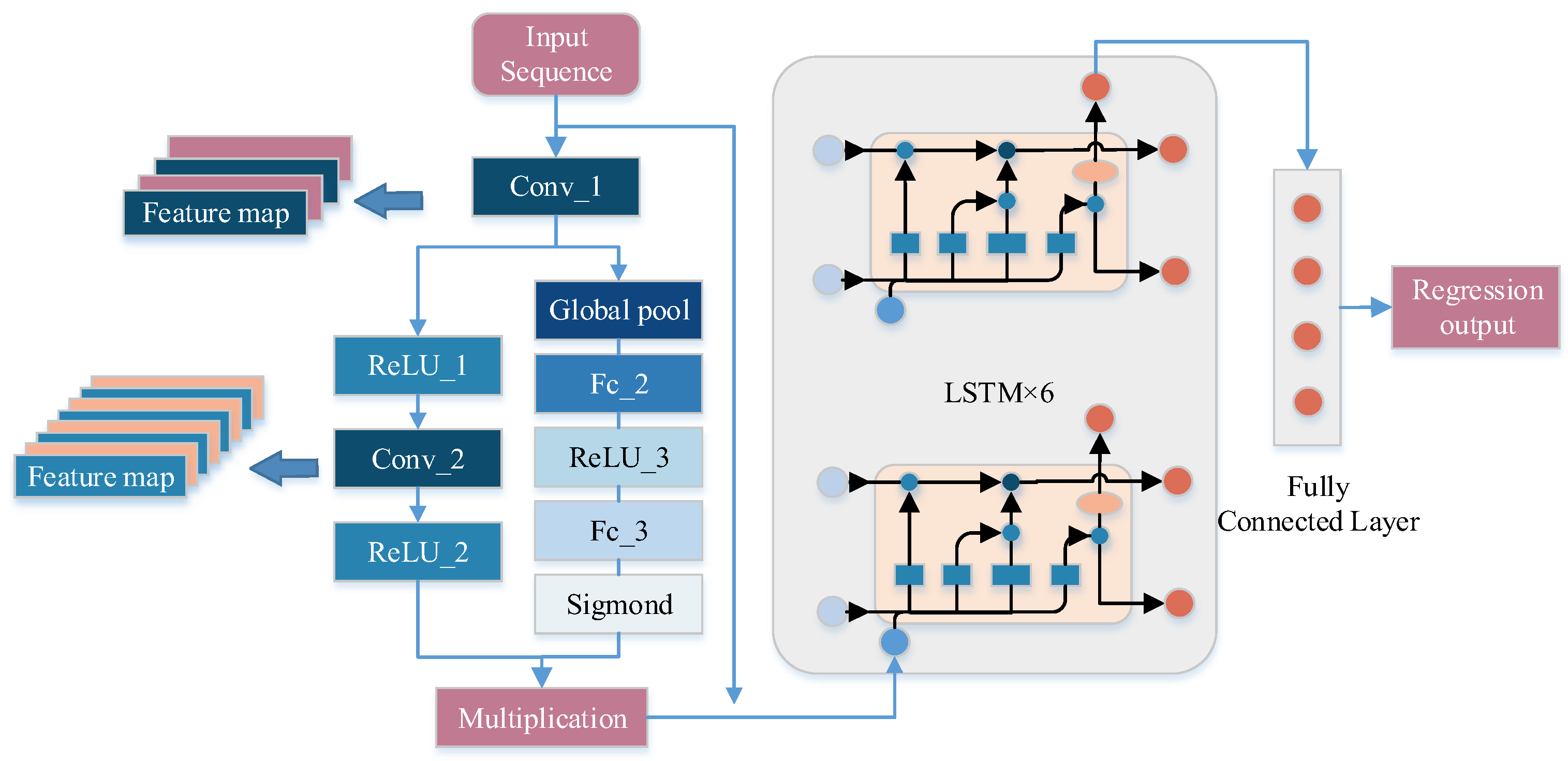
Since the dimension of the input features was not large in the design of the improved model, we designed the part of the CNN as a three-layer convolutional structure and fused the SE Attention Mechanism module through the short-circuit mechanism, and the Feature map after the convolutional neural network was used as the input of the LSTM. The increase in the number of implicit layers of the LSTM promoted the prediction performance of the model, which increased the amount of computation, but, unfortunately, did not affect the performance of the computer. Therefore, we set the number of LSTM hidden units to 8.
As shown in Figure 3, we preprocessed M × N sequences of historical meteorological data and condition indices and used them as input sequences for this model. In the CNN layer, we set the convolution kernel as 2 convolutional layers of 3 × 1 and the pooling kernel as 2 maximal pooling layers of 5 × 5. The activation function of the convolutional layer is ReLU function and the padding was set to the same. The pooling layer took the overall statistical features of the regions adjacent to a position of the input matrix as the output for that position, with the aim of reducing the number of nodes in the fully connected layer and thus simplifying the network parameters. The convolutional layer and the pooling layer together formed a feature extractor that can maximize the potential information of the input values to be reasonably extracted and also reduce the bias that occurs when the data are extracted by human beings. Therefore, in this study, CNN was firstly used to extract features from the normalized data, and subsequently analyzed and predicted by the LSTM network. The data were extracted from the convolutional layer, as well as from the pooling layer, and the obtained joint feature map was fed into the LSTM layer of the neural network through the SE Attention Mechanism. The LSTM layer mainly learned the features extracted from the CNN layer. The model was built with 8 layers of hidden units to fully learn the extracted features.
When the data were input at moment t, the LSTM first went through the computation of the forgetting gate:
The value of the input gate was then passed:
The formula for the candidate memory cell was:
The current memory cell state value was:
Then the value of the output gate was:
So the final output of LSTM at moment t was:
In Equations (5)–(10), σ represents the sigmond activation function, and tanh is the hyperbolic tangent activation function. , , are the values of the forgetting gate, the input gate, and the output gate, respectively, and the weights of the forgetting gate, the input gate, the state gate, and the output gate are and the weights of the state gate and the output gate, respectively, and the weights and biases of the cell and output gates, respectively.
The training of neural networks was prone to overfitting. Once overfitting occurs, even the model showed a small loss function value and high accuracy in the training set, but when applied to the test set, not only was the loss value large, but also the prediction accuracy was low; so, in this case, the model had no practical significance [34]. Dropout randomly and temporarily set the neurons of the neural network to zero during the training process; that is, it “discarded” the output of these neurons. “Dropout” is the output of these neurons [35]. In this way, each time a forward propagation was performed, it was equivalent to training a different, smaller sub-network. This process was similar to randomly removing neurons during training, thus reducing the network overdependence on specific neurons. We therefore set 2 layers of Dropout (with the discard rate set to 0.3 and 0.5, respectively) to prevent overfitting during training.
The hardware device used for the model building process was a Dell laptop with Intel(R) Core(TM) CPU i5-8250U @1.60 GHz processor, 16 GB of RAM, Window10 operating system, and the software for data processing and network training was MATLAB 2022b.
2.4. Evaluation Metrics
Prediction performance evaluation indexes are criteria for evaluating the performance of peanut leaf spot disease index prediction models. In this study, the coefficient of determination (), mean absolute error (MAE), mean bias error (MBE), and root mean square error (RMSE) were used to evaluate the prediction accuracy of the disease prediction model.
reflected the degree of fit of the model, and the closer its value was to 1, the better the input explained the response, which was calculated as:
MAE was the mean of the absolute value error, which truly reflected the magnitude of the prediction error and was calculated as:
MBE reflected the average deviation between the predicted value and the true value. The indicator was directional with positive values indicating overestimation and negative values indicating underestimation, and was calculated using the formula:
RMSE took into account the variation in the actual value and measured the average magnitude of the error, which was calculated as:
In each of the above formulas denoted the test value, the actual value of the output at that moment; denoted the predicted value of the output through the model prediction; N was the number of samples in the test set; and denoted the sample mean.
3. Results
3.1. Model Optimization
An exponential scale was used to set the learning rate during the training process, and comparative experiments with different learning rates and number of training parameters were conducted. A larger learning rate may cause the model to converge faster during training. However, if the learning rate is too large, it may cause the model to oscillate around the optimal point or even fail to converge. On the contrary, a smaller learning rate may cause slower convergence or even fall into a local minimum and fail to continue learning. According to the results in Table 2, it can be seen that under the same number of training times, the improved network model outperforms the performance of other learning rates on the test set when the learning rate was 0.001, especially the reached 0.951. The MAE, MBE, and RMSE metrics that we were concerned about had different degrees of decrease in comparison with the learning rate of 0.01. On the contrary, if the learning rate was set to 0.0001, even though the model can converge quickly, there was anomalous performance of the model R2 with this hyperparameter.
For this study, we applied multiple inputs to develop the prediction model. Among the numerous meteorological metrics, such as dew point and precipitation data with rapidly changing gradients or the presence of noise, Stochastic Gradient Descent with Momentum (SGDM) optimizers were less adaptive to non-stationary data, while adaptive learning algorithms (such as the Adam optimizer) were more advantageous. In other words, the adaptivity of Adam may be more advantageous for different input features when they may have different scales or importance. Moreover, Adam introduced the concept of momentum, which served to accelerate convergence by considering an exponentially weighted moving average of the gradient to overcome local minima during training [36,37,38], which was useful for dealing with complex loss surfaces or avoiding falling into local minima.
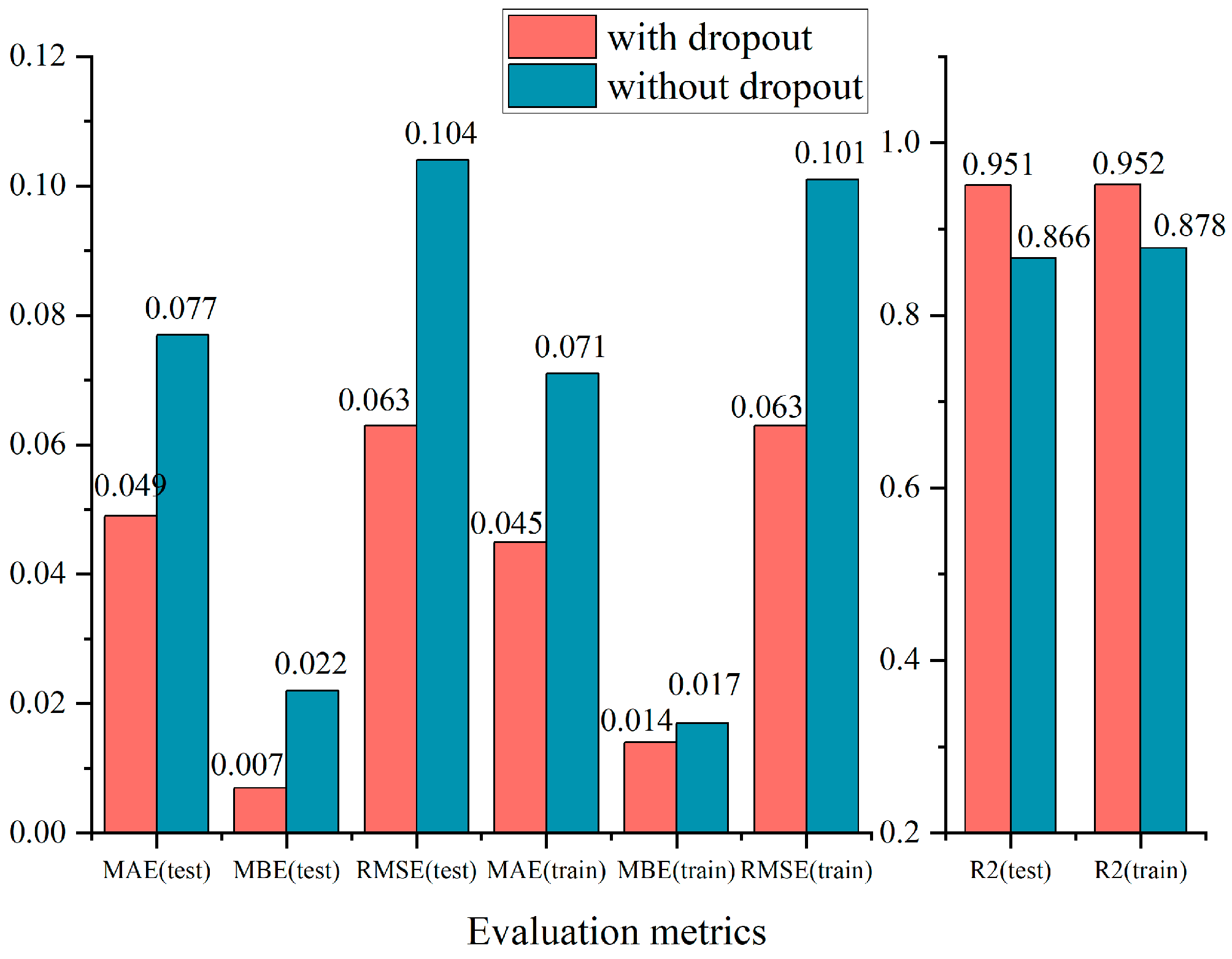
In addition, in order to reduce the interaction between LSTM hidden nodes and decrease the dependence on local features, we added dropout when designing the network. The results are displayed in Figure 4. When we regularized the network using dropout, MAE, MBE, and RMSE were 0.049, 0.007, and 0.063 on the test set, and reached 0.951. It was obvious that the addition of dropout decreased the test data by 0.028, 0.015, and 0.041 in MAE, MBE, and RMSE, respectively, and improved the by 0.085.
3.2. Disease Index Prediction
We constructed the weather data containing nine elements and the disease index and disease warning time as a dataset (weather data as input, and disease index and disease warning time as output), and divided them into a training set, test set, and validation set according to the ratio of 7:2:1 in the hold-out method [39]. After the training of the improved network, we obtained the prediction results on the training set and test set, respectively.
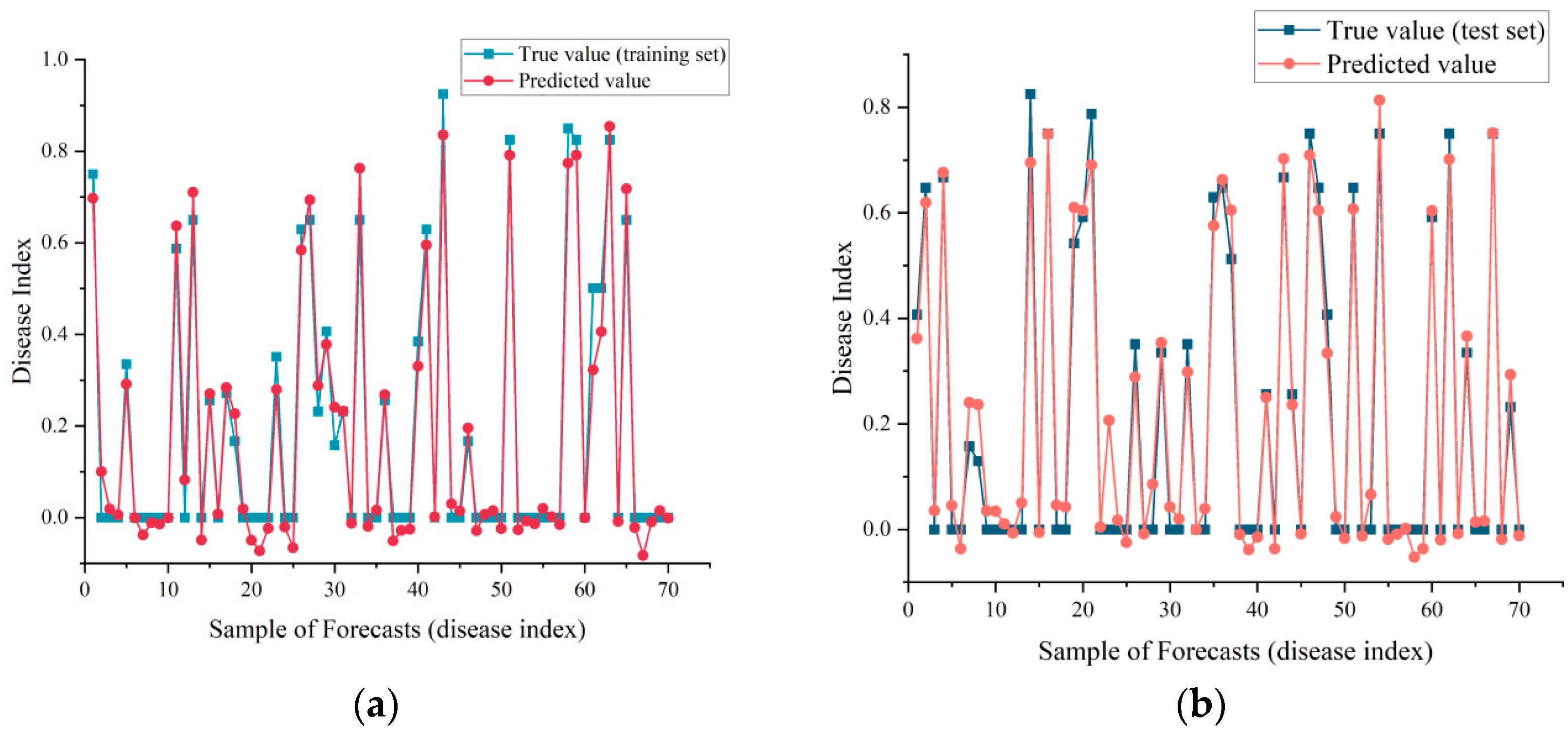
For disease index prediction, we observed that the model achieved disease index prediction with randomly disrupted samples. In Figure 5b, the prediction performance of the model for the test set data was subsequently not as good as that of the training set data in Figure 5a; overall, the true and predicted values matched well, and, fortunately, there was no overfitting such as poor accuracy on the test set.
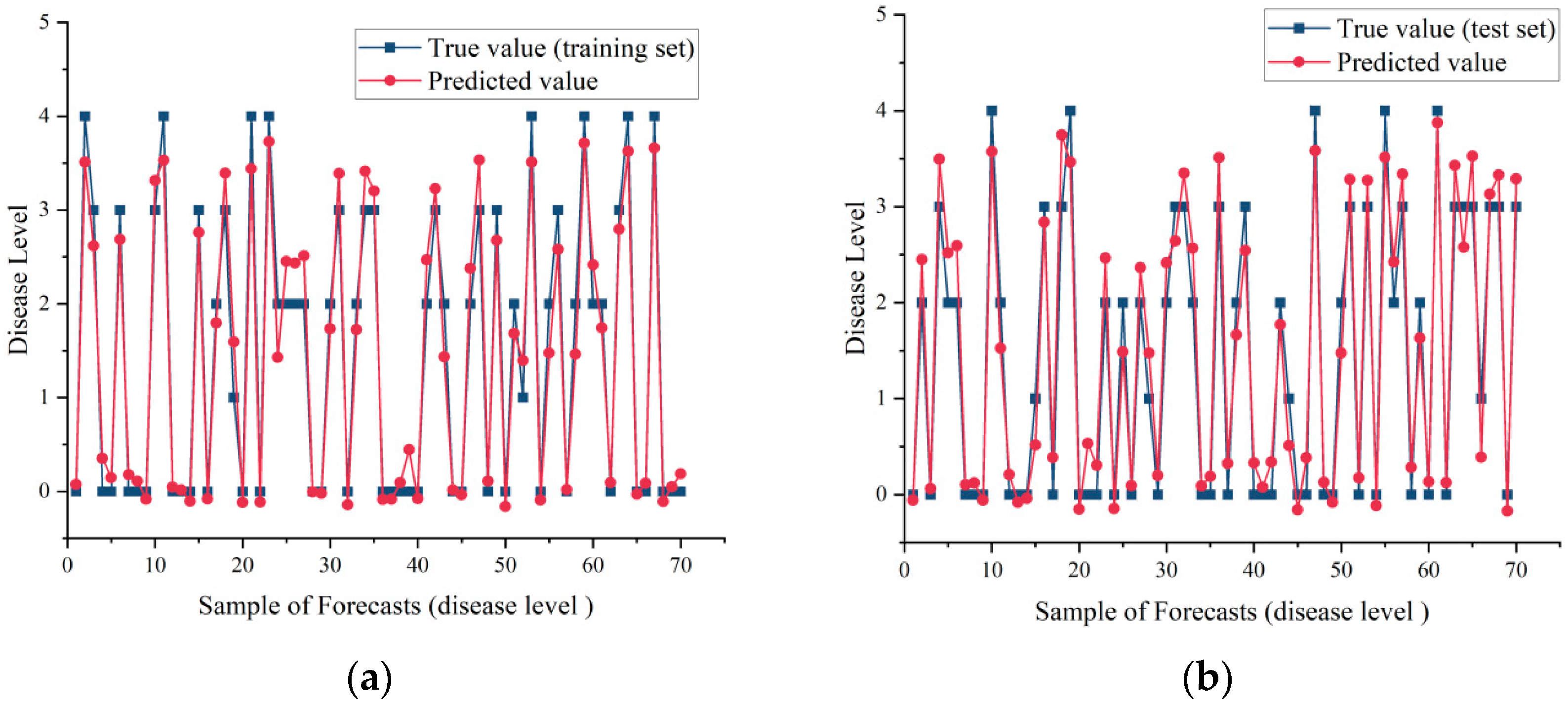
For the disease level, we also obtained better prediction results (Figure 6). We found that although there were differences in the prediction results of the improved network, the error was extremely small after we rounded the prediction results of the disease level, and by using the disease level zero and one, as well as the survey of onset times over the years, we could predict the disease level under future weather forecasts and subsequently infer the onset times.
3.3. Comparison of Prediction Models
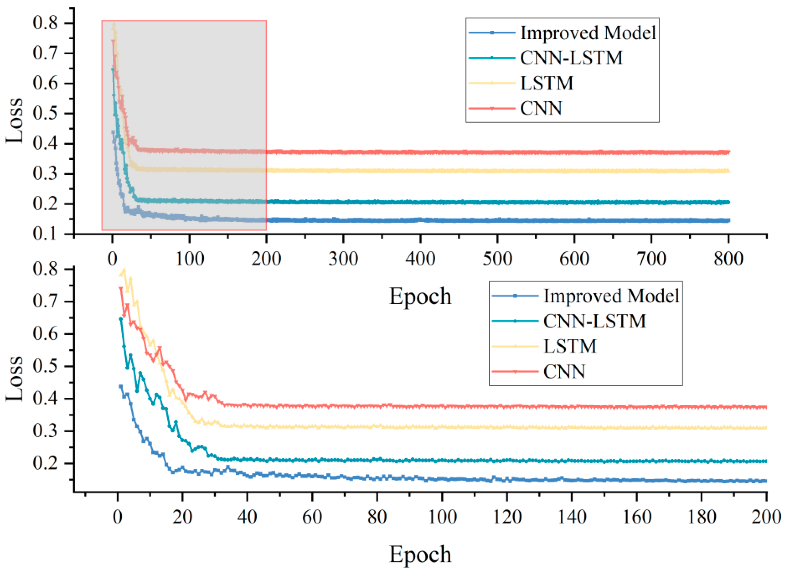
Since the improved model combines CNN, LSTM, and SE attention mechanisms, we compared the performance of CNN, LSTM, and the improved model under the same training parameters and environment. From Table 3, the performance of either the single CNN model or the LSTM model, or the CNN-LSTM model combining the two, was worse than the improved model. Focusing on the test data, the of the improved network was 0.121, 0.155, and 0.013 higher than that of the LSTM, CNN, and CNN-LSTM, in that order, and the RMSE decreased by 0.204, 0.253, and 0.019, in that order. In the loss curves of the training process, we observed that the loss of the improved model was consistently below that of the remaining three models. In particular, for the first 200 Epochs (bottom half of Figure 7), the improved model converged rapidly at the beginning of training (first 20 Epochs), and the loss still fluctuated up to 50 Epochs, and then decays and stabilizes at about 200 Epochs. The results indicated that the model achieved our expectations.
In addition, we included the classic BP neural network and the generalized regression neural network GRNN in the field of deep learning in the comparison. In order to ensure the rationality of the experiment, we also set the same training conditions (hardware environment and model hyperparameters). We found through Table 3 that the index of the GRNN model on the training set was as high as 0.994, which exceeded the improved model, but for the test set GRNN, was only 0.811, which was an anomalous performance through the actual test results. Therefore, we believed that the trained GRNN was in an overfitting state. For the BP neural network, the of the improved model was 0.496 higher, and the MAE, MBE, and RMSE decreased by 0.085, 0.007, and 0.155, respectively. Collectively, the improved model had the best performance in predicting peanut leaf spot disease.
3.4. Model Validation
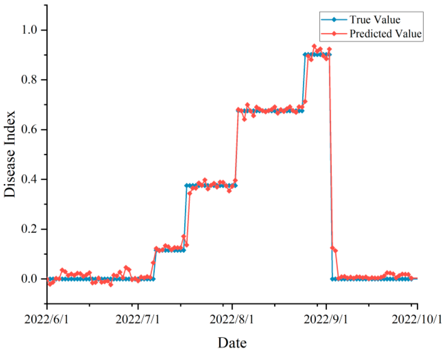
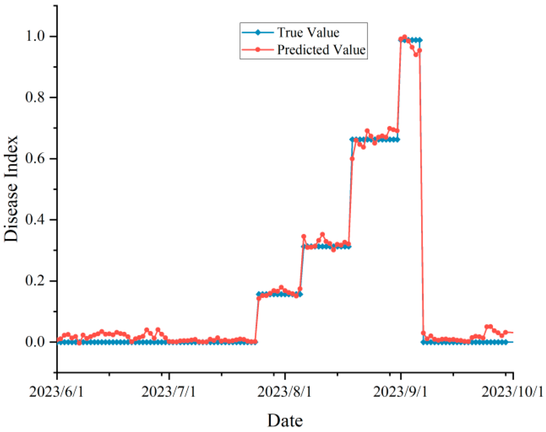
In order to practically test the robustness of our proposed model in real agricultural production scenarios, we investigated the peanut leaf spot disease occurrence in 2022 and 2023, and also obtained the meteorological data from June to September (peanut planting season) of these two years through the Open-Meteo interface. We used the day-by-day meteorological data and time series as inputs to the improved model, or to obtain the prediction results of the disease index, and compared them with the actual surveyed disease occurrence, and the validation results were shown in Figure 8 and Figure 9.
In the validation experiment, we predicted disease occurrence based on time scales (without randomly upsetting the data). Since the disease surveys in 2022 and 2023 were not conducted on a day-by-day basis, they were adjusted to a stage-specific disease index when the data were organized. From the figure, the predicted and actual values were highly consistent with each other, and there was no prediction abnormality, which proved that the proposed model was not overfitting and achieves our expected effect. According to the evaluation indexes, the , MAE, MBE, and RMSE of the data in 2022 were 0.932, 0.043, −0.018, and 0.067, respectively, and the indexes in 2023 were 0.938, 0.045, 0.012, and 0.052, respectively, which was a satisfactory result.
3.5. Sensitivity Analysis of the Proposed Model
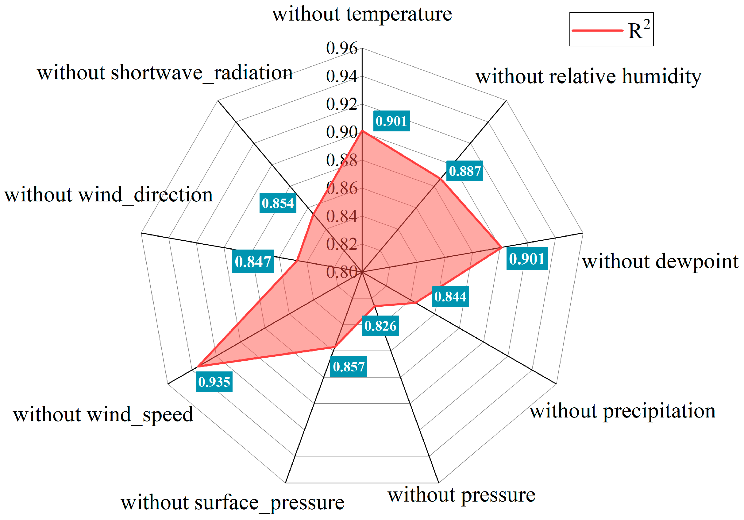
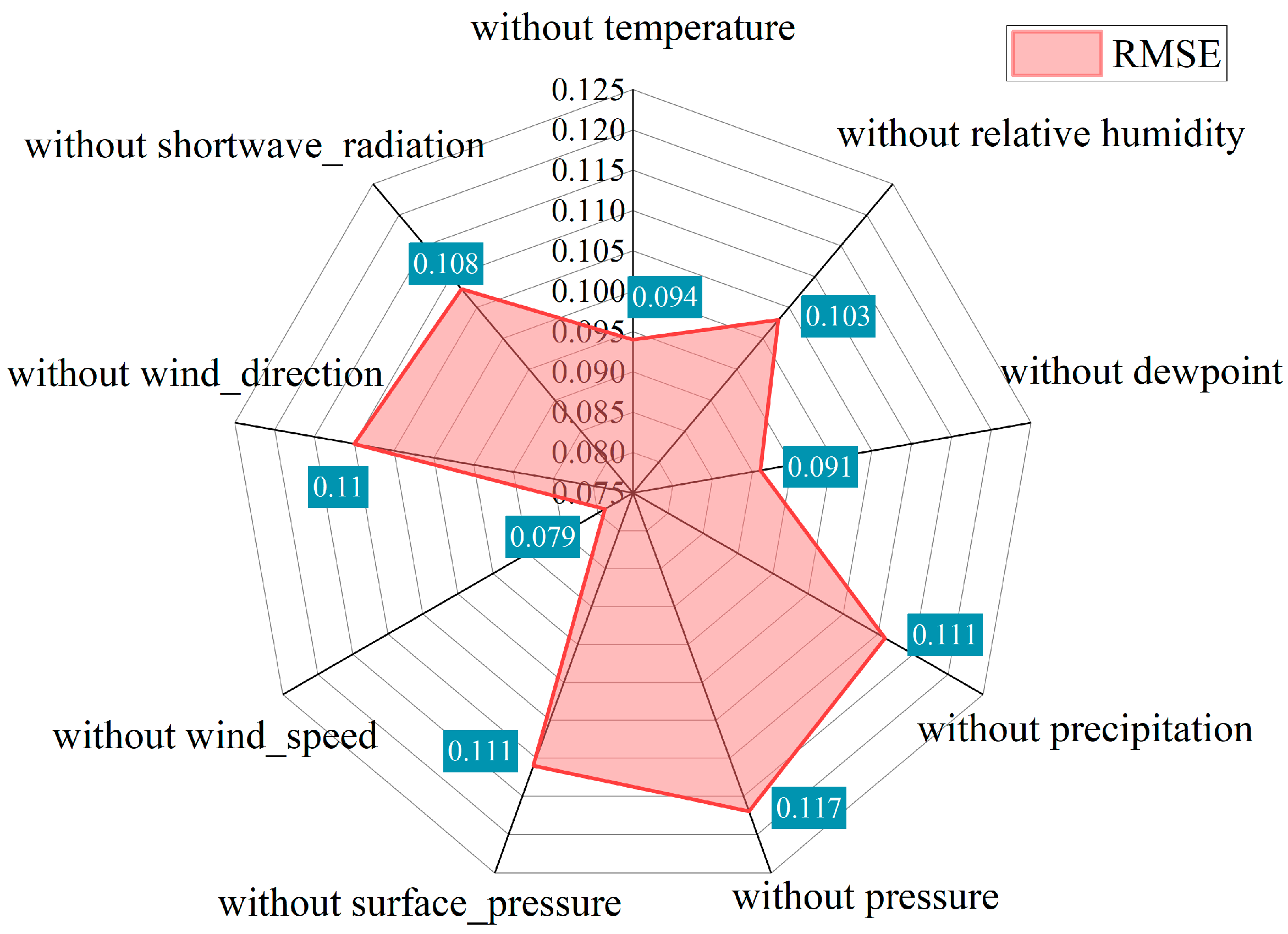
In order to gain a deeper understanding of the performance of the peanut leaf spot disease prediction model under the absence of different environmental variables, we retrained the model by masking out one weather element at a time and investigated the impact of each meteorological input feature on model performance metrics, particularly and RMSE. These findings are reflected in Figure 10 and Figure 11.
The results depicted in the figures unveil the intricate interplay between model prediction accuracy and the absence of individual meteorological data points. In Figure 10, a comprehensive examination of values revealed that excluding windspeed ( = 0.935) had the least adverse impact on the model, suggesting a relatively minor influence of this factor on disease prediction. Conversely, the exclusion of atmospheric pressure ( = 0.826) and relative humidity ( = 0.887) led to a more pronounced decrease in , emphasizing their crucial roles in the model. This indicated a substantial compromise in the model’s predictive ability when atmospheric pressure data were lacking, highlighting pressure as a key factor in understanding the atmospheric conditions influencing disease development. Furthermore, even with the omission of dewpoint data, the model exhibited a relatively high R2 value of 0.901, indicating robust performance despite the absence of this specific variable. The adaptability of the model to the absence of dewpoint data may be attributed to the intricate interactions captured by LSTM and SE networks, compensating for the missing information. In Figure 11, the RMSE values provided additional insights, where lower values signified more precise predictions. The marginal increase in RMSE after excluding windspeed (0.079) aligns with the analysis, further emphasizing the comparatively lower importance of wind speed. Conversely, the exclusion of atmospheric pressure and relative humidity resulted in elevated RMSE values, underscoring their critical roles in accurate disease prediction.
4. Discussion
The variability in meteorological patterns engenders microclimatic differences that significantly influence crop growth and the incidence of diseases, as observed in crops like soybeans [40], cucumbers [24], and peanuts [41]. Investigating the potential correlations between weather conditions and the prevalence of plant diseases is pivotal for the development of predictive models for these diseases [42]. A highlight of this study is the employment of data spanning five consecutive years for modeling, a relatively rare approach in the realm of predicting peanut leaf spot disease. This methodology enables a more comprehensive capture of long-term trends and patterns within the data, thereby enhancing the model’s generalizability and accuracy. Utilizing two years of data for validation purposes demonstrates the model’s stability and reliability across different time periods. In this research, we addressed the prediction of peanut leaf spot disease by synergizing an enhanced LSTM model with CNNs, and utilizing meteorological data. This integration aimed to meticulously capture the spatio-temporal features of the data, thus bolstering the model proficiency in discerning the dynamic nuances of the disease. Further, the incorporation of the SE Network Attention Mechanism module strategically focuses on pivotal features, significantly augmenting model performance.
We compared meteorological modeling methods with other approaches for predicting the prevalence of plant diseases. Liu [24] developed an LSTM-based predictive model using sensors in greenhouses, achieving a 95% accuracy rate in forecasting four environmental factors, which, in turn, predicted the occurrence of cucumber downy mildew. However, their model relied on single-factor inputs: one of our strengths was that the integration of multiple meteorological data provided richer features for the model. Similarly, Patle [43] utilized sensor data to establish an LSTM model for predicting mango diseases, attaining a 96% accuracy rate. Our predictive model, however, operates in open-air conditions, which, compared to the stable climate of greenhouses, presents greater data variability. Chen [44] framed the prediction of cotton pest occurrences as a time-series forecasting problem and applied a bidirectional LSTM model, achieving a prediction precision of 95%. Therefore, overall, employing LSTM for the establishment of a model to predict peanut leaf spot disease appears to be a justified approach.
The study delineated a substantial enhancement in predicting peanut leaf spot disease, surpassing traditional statistical methods. Our LSTM model, refined with CNN and SE networks, unraveled a more intricate understanding of plant disease dynamics. Table 3 showcased various models with their performance metrics (, MAE, MBE, RMSE) on both the test and training sets. The proposed model exhibited superior performance, particularly in terms of and RMSE, indicating a high degree of accuracy and consistency in prediction. The integration of CNN and LSTM benefited from the spatial feature extraction capability of CNNs and the temporal data processing strength of LSTMs. The addition of SE networks enhanced this by focusing on salient features, thus improving both predictive performance and interpretability. This model was likely more adept at identifying and emphasizing critical patterns linking meteorological conditions to disease outbreaks, offering valuable insights for agricultural decision making. This integration model eclipsed prior machine learning models in precision, attributable to its prowess in processing complex datasets and decoding intricate patterns emblematic of disease progression [45,46]. The standalone CNN and LSTM models showed lower performance metrics compared to the integrated approach. This suggested that while CNNs were adept at spatial feature extraction and LSTMs excelled in temporal data analysis, their combination leveraged these strengths synergistically. The integrated model captured complex spatial–temporal relationships more effectively, crucial for predicting diseases influenced by varying environmental factors. The integrated model’s high accuracy and low error metrics implied a deep understanding of the disease’s dynamics. This integrated approach resonated with findings in allied domains such as wind speed, energy consumption, and air quality prediction [47,48,49,50,51], corroborating our conclusion that the CNN-LSTM integrated model excels in performance. Additionally, through meticulous multi-parameter optimization, a model configuration with a learning rate of 0.001, a period (Epochs) of 800, and employing the Adam optimizer, demonstrated exceptional efficacy on the test set.
Furthermore, our study substantiated the feasibility and utility of a predictive methodology for peanut leaf spot disease grounded in meteorological conditions and neural networks. By scrutinizing historical meteorological data and disease survey records, we furnished agricultural practitioners with precise disease management insights, facilitating the formulation of efficacious control strategies to ameliorate the impact of diseases on crop yield. This innovative approach was integral to the realization of precision agriculture and the enhancement of crop yields. Employing meteorological data from the preceding two years as inputs to our model yielded predictions for peanut leaf spot disease with minimal deviation from actual manual survey records. This outcome attested to the model’s resilience against overfitting and its ability to render satisfactory predictions for the data of the years 2022 and 2023, which were not included in the training set (Figure 8 and Figure 9).
While our model exhibited encouraging outcomes, there were some shortcomings. Presently, the model was specifically tailored to the environmental and climatic nuances associated with peanut leaf spot disease. Adapting this model to other crops or varying geographical contexts may necessitate recalibrations, accommodating disparate disease dynamics and environmental variables. Our reliance on a constrained set of meteorological data and disease records prompted the exploration of additional data types, such as soil parameters and crop varietal information, in future research endeavors to enhance predictive precision. Moreover, there was a propensity for the model to exhibit hypersensitivity to certain attributes, potentially skewing predictions. To circumvent this, the exploration and implementation of advanced data augmentation techniques were warranted to bolster the model generalization capacity.
In summation, this research introduced a pioneering peanut leaf spot disease prediction methodology, amalgamating CNN, LSTM, and SE networks, and substantiated its efficacy and accuracy using empirical data. This novel approach furnishes farmers with an indispensable tool for disease management, propelling the aspirations of precision agriculture and diminishing disease-related losses. Future research trajectories may involve the refinement of the model architecture to optimize predictive accuracy and extend this methodology to a broader spectrum of crop disease prognostication.
5. Conclusions
For consecutive years of meteorological data and peanut leaf spot disease records, we investigated the use of CNN, SE Block, and LSTM to build a prediction model for peanut leaf spot disease. Among many deep learning models, by analyzing the relevance and expected goals of each module, we obtained an enhanced LSTM peanut leaf spot disease prediction model to predict its disease index and disease grade with and RMSE of 0.951 and 0.063, respectively. Through hyper-parameter optimization, it was established that when the learning rate was 0.001, the optimizer was Adam, and the number of cycles was 800, the improved network model achieved the best performance on the test set. The experimental results demonstrated that the use of meteorological data and the enhanced LSTM model had certain application value for timely and accurate prediction of peanut leaf spot disease, which could help growers make accurate management decisions and reduce disease impacts. In further studies, we will aim to explore the remaining environmental variables and crop physiological parameters used in plant disease prediction models.
Author Contributions
Conceptualization, D.S., Y.C. and M.L.; Methodology, M.L., Z.G. and D.S.; Software, D.S.; Validation, X.C. and Z.G.; Formal analysis, Z.G.; Investigation, D.S., Z.G. and X.C.; Resources, M.L. and Z.G.; Data curation, Z.G., X.C. and D.S.; Writing—original draft preparation, Z.G. and D.S.; Writing—review and editing, D.S.; Manuscript revising, Z.G. and M.L.; Study design, Z.G., X.C. and D.S.; Supervision, M.L., Y.C. and D.S.; Project administration, M.L. and Y.C.; Funding acquisition, Y.C. and M.L. All authors have read and agreed to the published version of the manuscript.
Funding
This research was funded by National Natural Science Foundation of China (31972967), National Key Technology Research and Development Program of China (2022YFE0199500), the EU FP7 Framework Program (PIRSES-GA-2013-612659), and Shandong Academy of Agricultural Sciences innovation project (CXGC2023G35).
Data Availability Statement
Data are contained within the article.
Conflicts of Interest
The authors declare no conflicts of interest.
References
- Giordano, D.F.; Pastor, N.; Palacios, S.; Oddino, C.M.; Torres, A.M. Peanut leaf spot caused by Nothopassalora personata. Trop. Plant Pathol. 2021, 46, 139–151. [Google Scholar] [CrossRef]
- Kundu, N.; Rani, G.; Dhaka, V.S.; Gupta, K.; Nayak, S.C.; Verma, S.; Ijaz, M.F.; Woźniak, M. IoT and interpretable machine learning based framework for disease prediction in pearl millet. Sensors 2021, 21, 5386. [Google Scholar] [CrossRef] [PubMed]
- Fulmer, A.M.; Mehra, L.K.; Kemerait, R.C., Jr.; Brenneman, T.B.; Culbreath, A.K.; Stevenson, K.L.; Cantonwine, E.G. Relating Peanut Rx risk factors to epidemics of early and late leaf spot of peanut. Plant Dis. 2019, 103, 3226–3233. [Google Scholar] [CrossRef] [PubMed]
- Kankam, F.; Akpatsu, I.B.; Tengey, T.K. Leaf spot disease of groundnut: A review of existing research on management strategies. Cogent Food Agric. 2022, 8, 2118650. [Google Scholar] [CrossRef]
- Paredes, J.A.; Edwards Molina, J.P.; Cazón, L.I.; Asinari, F.; Monguillot, J.H.; Morichetti, S.A.; Rago, A.M.; Torres, A.M. Relationship between incidence and severity of peanut smut and its regional distribution in the main growing region of Argentina. Trop. Plant Pathol. 2021, 47, 233–244. [Google Scholar] [CrossRef]
- Buja, I.; Sabella, E.; Monteduro, A.G.; Chiriacò, M.S.; De Bellis, L.; Luvisi, A.; Maruccio, G. Advances in plant disease detection and monitoring: From traditional assays to in-field diagnostics. Sensors 2021, 21, 2129. [Google Scholar] [CrossRef] [PubMed]
- Martinelli, F.; Scalenghe, R.; Davino, S.; Panno, S.; Scuderi, G.; Ruisi, P.; Villa, P.; Stroppiana, D.; Boschetti, M.; Goulart, R.L.; et al. Advanced methods of plant disease detection: A review. Agron. Sustain. Dev. 2015, 35, 1–25. [Google Scholar] [CrossRef]
- Patil, R.R.; Kumar, S. Predicting rice diseases across diverse agro-meteorological conditions using an artificial intelligence approach. PeerJ Comput. Sci. 2021, 7, e687. [Google Scholar] [CrossRef]
- Islam, M.M.; Adil, M.A.A.; Talukder, M.A.; Ahamed, M.K.U.; Uddin, M.A.; Hasan, M.K.; Sharmin, S.; Rahman, M.; Debnath, S.K. DeepCrop: Deep learning-based crop disease prediction with web application. J. Agric. Food Res. 2023, 14, 100764. [Google Scholar] [CrossRef]
- Fenu, G.; Malloci, F.M. Forecasting plant and crop disease: An explorative study on current algorithms. Big Data Cogn. Comput. 2021, 5, 2. [Google Scholar] [CrossRef]
- Azadbakht, M.; Ashourloo, D.; Aghighi, H.; Radiom, S.; Alimohammadi, A. Wheat leaf rust detection at canopy scale under different LAI levels using machine learning techniques. Comput. Electron. Agric. 2019, 156, 119–128. [Google Scholar] [CrossRef]
- Guan, Q.; Zhao, D.; Feng, S.; Xu, T.; Wang, H.; Song, K. Hyperspectral Technique For Detection Of Peanut Leaf Spot Disease Based On Improved PCA Loading. Agronomy 2023, 13, 1153. [Google Scholar] [CrossRef]
- Bhatia, A.; Chug, A.; Singh, A.P. Application of extreme learning machine in plant disease prediction for highly imbalanced dataset. J. Stat. Manag. Syst. 2020, 23, 1059–1068. [Google Scholar] [CrossRef]
- Xiao, Q.; Li, W.; Chen, P.; Wang, B. Prediction of crop pests and diseases in cotton by long short term memory network. In Intelligent Computing Theories and Application: Proceedings of the 14th International Conference, ICIC 2018, Wuhan, China, 15–18 August 2018; Proceedings, Part II 14; Springer International Publishing: New York, NY, USA, 2018; pp. 11–16. [Google Scholar]
- Ji, T.; Languasco, L.; Li, M.; Rossi, V. Effects of temperature and wetness duration on infection by Coniella diplodiella, the fungus causing white rot of grape berries. Plants 2021, 10, 1696. [Google Scholar] [CrossRef]
- Ji, T.; Salotti, I.; Dong, C.; Li, M.; Rossi, V. Modeling the effects of the environment and the host plant on the ripe rot of grapes, caused by the Colletotrichum species. Plants 2021, 10, 2288. [Google Scholar] [CrossRef] [PubMed]
- Juroszek, P.; Racca, P.; Link, S.; Farhumand, J.; Kleinhenz, B. Overview on the review articles published during the past 30 years relating to the potential climate change effects on plant pathogens and crop disease risks. Plant Pathol. 2020, 69, 179–193. [Google Scholar] [CrossRef]
- Benos, L.; Tagarakis, A.C.; Dolias, G.; Berruto, R.; Kateris, D.; Bochtis, D. Machine learning in agriculture: A comprehensive updated review. Sensors 2021, 21, 3758. [Google Scholar] [CrossRef]
- Bhagawati, R.; Bhagawati, K.; Singh, A.K.K.; Nongthombam, R.; Sarmah, R.; Bhagawati, G. Artificial neural network assisted weather based plant disease forecasting system. Int. J. Recent Innov. Trends Comput. Commun. 2015, 3, 4168–4173. [Google Scholar]
- Prank, M.; Kenaley, S.C.; Bergstrom, G.C.; Acevedo, M.; Mahowald, N.M. Climate change impacts the spread potential of wheat stem rust, a significant crop disease. Environ. Res. Lett. 2019, 14, 124053. [Google Scholar] [CrossRef]
- Fenu, G.; Malloci, F.M. An application of machine learning technique in forecasting crop disease. In Proceedings of the 3rd International Conference on Big Data Research, Cergy-Pontoise, France, 20–22 November 2019; pp. 76–82. [Google Scholar]
- Fenu, G.; Malloci, F.M. Artificial intelligence technique in crop disease forecasting: A case study on potato late blight prediction. In Intelligent Decision Technologies: Proceedings of the 12th KES International Conference on Intelligent Decision Technologies (KES-IDT 2020), Virtual, 17–19 June 2020; Springer: Singapore, 2020; pp. 79–89. [Google Scholar]
- Kim, Y.; Roh, J.-H.; Kim, H.Y. Early forecasting of rice blast disease using long short-term memory recurrent neural networks. Sustainability 2017, 10, 34. [Google Scholar] [CrossRef]
- Liu, K.; Zhang, C.; Yang, X.; Diao, M.; Liu, H.; Li, M. Development of an Occurrence Prediction Model for Cucumber Downy Mildew in Solar Greenhouses Based on Long Short-Term Memory Neural Network. Agronomy 2022, 12, 442. [Google Scholar] [CrossRef]
- Liu, K.; Mu, Y.; Chen, X.; Ding, Z.; Song, M.; Xing, D.; Li, M. Towards developing an epidemic monitoring and warning system for diseases and pests of hot peppers in Guizhou, China. Agronomy 2022, 12, 1034. [Google Scholar] [CrossRef]
- Huang, Y.; Zhang, J.; Zhang, J.; Yuan, L.; Zhou, X.; Xu, X.; Yang, G. Forecasting Alternaria Leaf Spot in Apple with Spatial-Temporal Meteorological and Mobile Internet-Based Disease Survey Data. Agronomy 2022, 12, 679. [Google Scholar] [CrossRef]
- Janiesch, C.; Zschech, P.; Heinrich, K. Machine learning and deep learning. Electron. Mark. 2021, 31, 685–695. [Google Scholar] [CrossRef]
- Dargan, S.; Kumar, M.; Ayyagari, M.R.; Kumar, G. A survey of deep learning and its applications: A new paradigm to machine learning. Arch. Comput. Methods Eng. 2020, 27, 1071–1092. [Google Scholar] [CrossRef]
- Hecht-Nielsen, R. Theory of the backpropagation neural network. In Neural Networks for Perception; Academic Press: Cambridge, MA, USA, 1992; pp. 65–93. [Google Scholar]
- Specht, D.F. A general regression neural network. IEEE Trans. Neural Netw. 1991, 2, 568–576. [Google Scholar] [CrossRef] [PubMed]
- Chiteka, Z.A.; Gorbet, D.W.; Shokes, F.M.; Kucharek, T.A.; Knauft, D.A. Components of resistance to late leafspot in peanut. I. Levels and variability-implications for selection. Peanut Sci. 1988, 15, 25–30. [Google Scholar] [CrossRef]
- Hu, J.; Shen, L.; Sun, G. Squeeze-and-excitation networks. In Proceedings of the IEEE Conference on Computer Vision and Pattern Recognition, Salt Lake City, UT, USA, 18–22 June 2018; pp. 7132–7141. [Google Scholar]
- Jin, X.; Xie, Y.; Wei, X.S.; Zhao, B.R.; Chen, Z.M.; Tan, X. Delving deep into spatial pooling for squeeze-and-excitation networks. Pattern Recognit. 2022, 121, 108159. [Google Scholar] [CrossRef]
- Ying, X. An overview of overfitting and its solutions. J. Phys. Conf. Ser. 2019, 1168, 022022. [Google Scholar] [CrossRef]
- Poernomo, A.; Kang, D.-K. biased dropout and crossmap dropout: Learning towards effective dropout regularization in convolutional neural network. Neural Netw. 2018, 104, 60–67. [Google Scholar] [CrossRef]
- Postalcıoğlu, S. Performance analysis of different optimizers for deep learning-based image recognition. Int. J. Pattern Recognit. Artif. Intell. 2020, 34, 2051003. [Google Scholar] [CrossRef]
- Kingma, D.P.; Ba, J. Adam: A method for stochastic optimization. arXiv 2014, arXiv:1412.6980. [Google Scholar]
- Dogo, E.M.; Afolabi, O.J.; Nwulu, N.I.; Twala, B.; Aigbavboa, C.O. A comparative analysis of gradient descent-based optimization algorithms on convolutional neural networks. In Proceedings of the 2018 International Conference on Computational Techniques, Electronics and Mechanical Systems (CTEMS), Belagavi, India, 21–23 December 2018; pp. 92–99. [Google Scholar]
- Larcher, C.H.; Barbosa, H.J. Evaluating Models with Dynamic Sampling Holdout. In Applications of Evolutionary Computation: Proceedings of the 24th International Conference, EvoApplications 2021, Held as Part of EvoStar 2021, Virtual Event, 7–9 April 2021; Proceedings 24; Springer International Publishing: New York, NY, USA, 2021; pp. 729–744. [Google Scholar]
- Bhamra, G.K.; Borah, M.; Borah, P.K. Rhizoctonia Aerial Blight of Soybean, its Prevalence and Epidemiology: A Review. Agricultural 2022, 43, 463–468. [Google Scholar] [CrossRef]
- Barocco, R.L.; Sanjel, S.; Dufault, N.S.; Barrett, C.; Broughton, B.; Wright, D.L.; Small, I.M. Peanut Disease Epidemiology under Dynamic Microclimate Conditions and Management Practices in North Florida. Plant Dis. 2021, 105, 2333–2342. [Google Scholar] [CrossRef]
- Jain, S.; Ramesh, D. AI based hybrid CNN-LSTM model for crop disease prediction: An ML advent for rice crop. In Proceedings of the 2021 12th International Conference on Computing Communication and Networking Technologies (ICCCNT), Kharagpur, India, 6–8 July 2021; pp. 1–7. [Google Scholar]
- Patle, K.S.; Saini, R.; Kumar, A.; Palaparthy, V.S. Field evaluation of smart sensor system for plant disease prediction using lstm network. IEEE Sens. J. 2021, 22, 3715–3725. [Google Scholar] [CrossRef]
- Chen, P.; Xiao, Q.; Zhang, J.; Xie, C.; Wang, B. Occurrence prediction of cotton pests and diseases by bidirectional long short-term memory networks with climate and atmosphere circulation. Comput. Electron. Agric. 2020, 176, 105612. [Google Scholar] [CrossRef]
- Kim, T.-Y.; Cho, S.-B. Predicting residential energy consumption using CNN-LSTM neural networks. Energy 2019, 182, 72–81. [Google Scholar] [CrossRef]
- Chung, W.H.; Gu, Y.H.; Yoo, S.J. District heater load forecasting based on machine learning and parallel CNN-LSTM attention. Energy 2022, 246, 123350. [Google Scholar] [CrossRef]
- Tang, J.; Li, Y.; Ding, M.; Liu, H.; Yang, D.; Wu, X. An ionospheric tec forecasting model based on a CNN-LSTM-attention mechanism neural network. Remote Sens. 2022, 14, 2433. [Google Scholar] [CrossRef]
- Wan, A.; Chang, Q.; Al-Bukhaiti, K.; He, J. Short-term power load forecasting for combined heat and power using CNN-LSTM enhanced by attention mechanism. Energy 2023, 282, 128274. [Google Scholar] [CrossRef]
- Livieris, I.E.; Pintelas, E.; Pintelas, P. A CNN–LSTM model for gold price time-series forecasting. Neural Comput. Appl. 2020, 32, 17351–17360. [Google Scholar] [CrossRef]
- Elmaz, F.; Eyckerman, R.; Casteels, W.; Latré, S.; Hellinckx, P. CNN-LSTM architecture for predictive indoor temperature modeling. Build. Environ. 2021, 206, 108327. [Google Scholar] [CrossRef]
- Yan, R.; Liao, J.; Yang, J.; Sun, W.; Nong, M.; Li, F. Multi-hour and multi-site air quality index forecasting in Beijing using CNN, LSTM, CNN-LSTM, and spatiotemporal clustering. Expert Syst. Appl. 2021, 169, 114513. [Google Scholar] [CrossRef]
Figure 1.
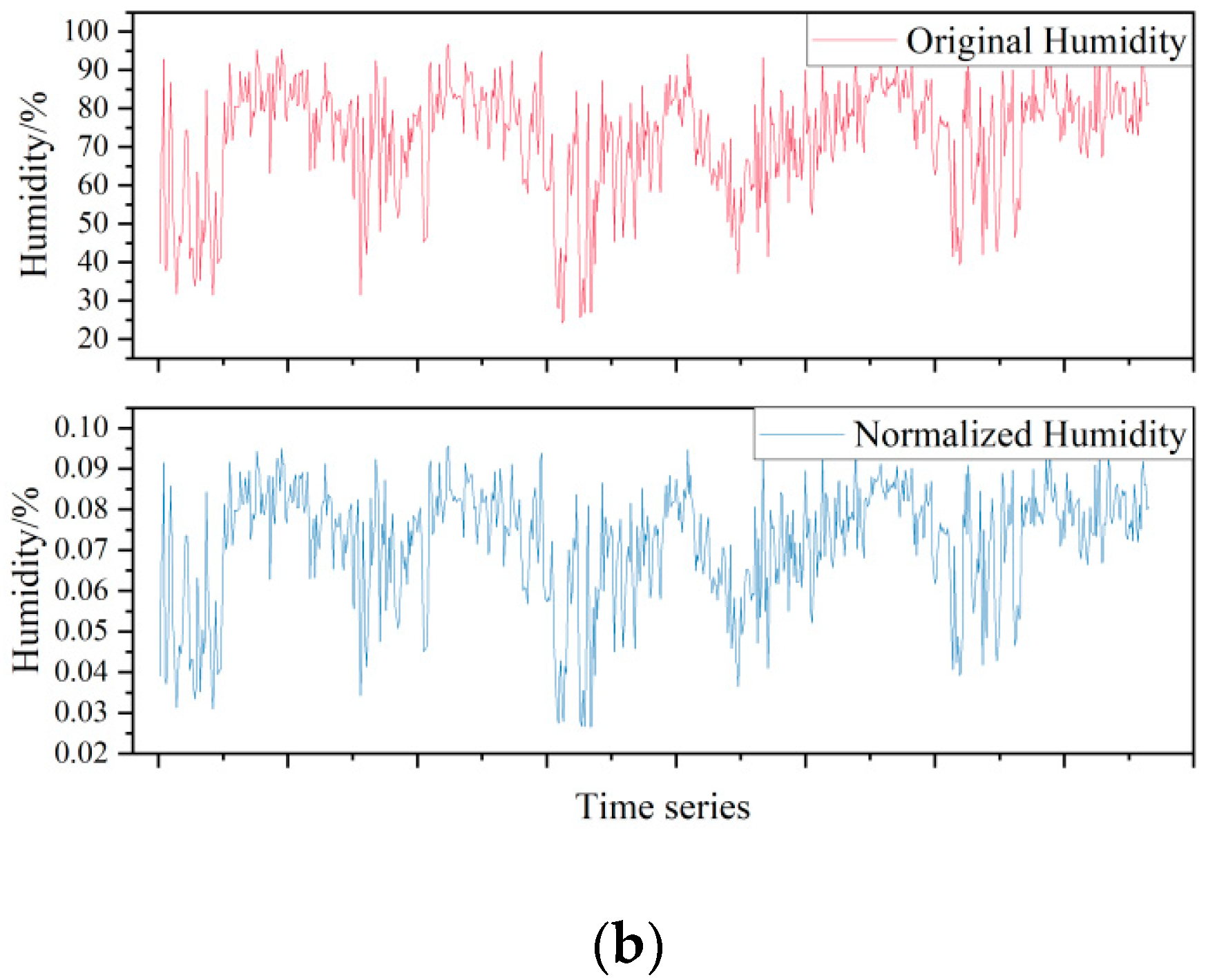
Comparison of curves before and after data normalization: (a) Temperature. (b) Relative humidity.
Figure 1.
Comparison of curves before and after data normalization: (a) Temperature. (b) Relative humidity.


Figure 2.
SE Block structure. The first orange square indicates the feature before regular convolution and the blue square indicates the feature after regular ordinary convolution. The last colored square represents the features output by SE Networks. Note: is the conventional convolution; denotes the squeeze operation; is the excitation operation.

Figure 3.
Structure of the improved network model. Feature map represents the features of the convolution operation; Conv represents the convolution operation, ReLU and Sigmond represent the activation functions; Fc represents the fully connected operation.
Figure 3.
Structure of the improved network model. Feature map represents the features of the convolution operation; Conv represents the convolution operation, ReLU and Sigmond represent the activation functions; Fc represents the fully connected operation.

Figure 4.
Effect of dropout on model performance. Red blocks represented the addition of a dropout layer to the proposed model; blue blocks represented the absence of a dropout layer. Smaller values of MAE, MBE, and RMSE implied smaller prediction errors. Higher values of represented higher prediction accuracy. Note: The values on the graph represented specific evaluation indicators for the model.

Figure 5.
Disease index prediction results: (a) Training set prediction results; (b) Test set prediction results. The red line represented the model’s predicted value and the blue line represented the true value.
Figure 5.
Disease index prediction results: (a) Training set prediction results; (b) Test set prediction results. The red line represented the model’s predicted value and the blue line represented the true value.

Figure 6.
Results of disease level prediction: (a) Training set prediction results; (b) Test set prediction results. The red line represented the model’s predicted value and the blue line represented the true value.
Figure 6.
Results of disease level prediction: (a) Training set prediction results; (b) Test set prediction results. The red line represented the model’s predicted value and the blue line represented the true value.

Figure 7.
Training loss curves for different models. The bottom half was a detailed plot of the training losses of the first 200 epochs after zooming in, making it easy to observe the convergence rate of each model.
Figure 7.
Training loss curves for different models. The bottom half was a detailed plot of the training losses of the first 200 epochs after zooming in, making it easy to observe the convergence rate of each model.

Figure 8.
Disease prediction and actual validation in 2022. The red line represents the model’s predicted value and the blue line represents the true value.
Figure 8.
Disease prediction and actual validation in 2022. The red line represents the model’s predicted value and the blue line represents the true value.

Figure 9.
Disease prediction and actual validation in 2023. The red line represented the model’s predicted value and the blue line represented the true value.
Figure 9.
Disease prediction and actual validation in 2023. The red line represented the model’s predicted value and the blue line represented the true value.

Figure 10.
radar plot for sensitivity analysis of meteorological data to the model.

Figure 11.
RMSE radar plot for sensitivity analysis of meteorological data to the model.


Table 1.
Leaf spot scoring system used for plant appearance score.
| Disease Level | Description |
|---|---|
| 0 | No disease |
| 1 | The lower leaves of the peanut plants having small necrotic spots or a small number of necrotic spots (none on upper canopy) |
| 2 | More lesions on the lower leaves and obvious lesions on the middle leaves |
| 3 | The middle and lower leaves of the peanut plant having more necrotic-spots and slight defoliation, and the upper leaves having necrotic spots |
| 4 | The upper, middle, and lower leaves of the peanut plant covered with necrotic spots and noticeable defoliation |
Table 2.
Effect of different learning rates on model performance.
| Learning Rate | Test Set | Training Set | ||||||
|---|---|---|---|---|---|---|---|---|
| MAE | MBE | RMSE | MAE | MBE | RMSE | |||
| 0.01 | 0.907 | 0.059 | 0.005 | 0.071 | 0.914 | 0.050 | 0.003 | 0.052 |
| 0.001 | 0.951 | 0.049 | 0.006 | 0.063 | 0.952 | 0.045 | 0.014 | 0.063 |
| 0.0001 | 0.532 | 0.138 | 0.012 | 0.196 | 0.552 | 0.141 | 0.002 | 0.193 |
Table 3.
Comparison of the performance of different models for predicting peanut leaf spot disease.
| Model | Test Set | Training Set | ||||||
|---|---|---|---|---|---|---|---|---|
| MAE | MBE | RMSE | MAE | MBE | RMSE | |||
| CNN-LSTM | 0.938 | 0.052 | 0.016 | 0.082 | 0.983 | 0.031 | 0.002 | 0.047 |
| LSTM | 0.830 | 0.184 | 0.146 | 0.267 | 0.845 | 0.139 | 0.113 | 0.221 |
| CNN | 0.796 | 0.235 | −0.205 | 0.316 | 0.802 | 0.218 | −0.197 | 0.302 |
| GRNN | 0.811 | 0.048 | −0.004 | 0.120 | 0.994 | 0.010 | −0.001 | 0.023 |
| BP Network | 0.455 | 0.134 | 0.014 | 0.218 | 0.509 | 0.120 | 0.007 | 0.199 |
| Ours | 0.951 | 0.049 | 0.007 | 0.063 | 0.952 | 0.045 | 0.014 | 0.063 |
Disclaimer/Publisher’s Note: The statements, opinions and data contained in all publications are solely those of the individual author(s) and contributor(s) and not of MDPI and/or the editor(s). MDPI and/or the editor(s) disclaim responsibility for any injury to people or property resulting from any ideas, methods, instructions or products referred to in the content. |
© 2024 by the authors. Licensee MDPI, Basel, Switzerland. This article is an open access article distributed under the terms and conditions of the Creative Commons Attribution (CC BY) license (https://creativecommons.org/licenses/by/4.0/).
Share and Cite
MDPI and ACS Style
Guo, Z.; Chen, X.; Li, M.; Chi, Y.; Shi, D. Construction and Validation of Peanut Leaf Spot Disease Prediction Model Based on Long Time Series Data and Deep Learning. Agronomy 2024, 14, 294. https://doi.org/10.3390/agronomy14020294
AMA Style
Guo Z, Chen X, Li M, Chi Y, Shi D. Construction and Validation of Peanut Leaf Spot Disease Prediction Model Based on Long Time Series Data and Deep Learning. Agronomy. 2024; 14(2):294. https://doi.org/10.3390/agronomy14020294
Chicago/Turabian StyleGuo, Zhiqing, Xiaohui Chen, Ming Li, Yucheng Chi, and Dongyuan Shi. 2024. "Construction and Validation of Peanut Leaf Spot Disease Prediction Model Based on Long Time Series Data and Deep Learning" Agronomy 14, no. 2: 294. https://doi.org/10.3390/agronomy14020294
Note that from the first issue of 2016, this journal uses article numbers instead of page numbers. See further details here.