Integration of Deep Learning and Sparrow Search Algorithms to Optimize Greenhouse Microclimate Prediction for Seedling Environment Suitability

Abstract

The climatic parameters within greenhouse facilities, such as temperature, humidity, and light, exert significant influence on the growth and yield of crops, particularly seedlings. Therefore, it is crucial to establish an accurate predictive model to monitor and adjust the greenhouse microclimate for optimizing the greenhouse environment to the fullest extent. To precisely forecast the greenhouse microclimate and assess the suitability of nursery environments, this study focuses on greenhouse environmental factors. This study leveraged open-source APIs to acquire meteorological data, integrated a model based on Convolutional Neural Networks (CNN) and Long Short-Term Memory Networks (LSTM), and utilized the sparrow search algorithm to optimize model parameters, consequently developing a time series greenhouse microclimate prediction model. Furthermore, Squeeze-and-Excitation (SE) Networks were employed to enhance the model’s attention mechanism, enabling more accurate predictions of environmental factors within the greenhouse. The predictive results indicated that the optimized model achieved high precision in forecasting the greenhouse microclimate, with average errors of 0.540 °C, 0.936%, and 1.586 W/m² for temperature, humidity, and solar radiation, respectively. The coefficients of determination (${\mathrm{R}}^2$) reached 0.940, 0.951, and 0.936 for temperature, humidity, and solar radiation, respectively. In comparison to individual CNN or LSTM models, as well as the back-propagation (BP) neural network, the proposed model demonstrates a significant improvement in predictive accuracy. Moreover, this research was applied to the greenhouse nursery environment, demonstrating that the proposed model significantly enhanced the efficiency of greenhouse seedling cultivation and the quality of seedlings. Our study provided an effective approach for optimizing greenhouse environmental control and nursery environment suitability, contributing significantly to achieving sustainable and efficient agricultural production.

1. Introduction

In the current era, marked by escalating global climate change and food security challenges, greenhouse agriculture emerges as a pivotal technology for enhancing crop yield and quality. Compared to open field cultivation, greenhouses offer the advantage of facilitating optimal plant growth conditions and a more uniform environment [1,2]. Key environmental factors within greenhouses, such as temperature, humidity, and solar radiation, are recognized as primary components associated with the microclimate effects of greenhouses [3], exerting a decisive influence on the growth and development of greenhouse crops. Adhering to the perspectives of Santini and Shahzad [4,5], maintaining temperature within an ideal range was crucial for crop growth. Studies also indicated [6,7] that relative humidity and solar radiation played significant roles in crop development within greenhouse settings. Accurate prediction of these environmental factors was therefore essential to ensure optimal growing conditions for crops, minimize resource wastage, perpetuate sustainable agriculture, and meet the challenges posed by climate extremes.

Greenhouses, as nonlinear and temporally variant microsystems, were influenced by external climatic changes, internal crop physiology, and human interventions. Early studies in greenhouse microclimate simulation were dominated by mechanistic models [8,9,10]. However, these models often required extensive parameter collection, directly impacting their fit and efficacy [11]. The evolution of computer technology had infused new vitality into greenhouse microclimate simulation; deep learning approaches, considering multiple indoor and outdoor factors, achieved precise predictions [12,13,14,15,16]. For instance, Hong et al. [17] developed an Elman recurrent neural network model to predict temperature and humidity in greenhouses, utilizing a momentum BP algorithm to modify connection weights for reducing prediction errors and enhancing learning capacity. Petrakis et al. [12] emphasized the significance of maintaining the appropriate greenhouse environment using a computational decision support system (DSS). They developed a multilayer perceptron neural network (MLP-NN) utilizing Levenberg–Marquardt backpropagation for modeling the internal temperature and relative humidity of an agricultural greenhouse. Similarly, Gharghory et al. [18] proposed an enhanced architecture of a recurrent neural network based on LSTM for predicting greenhouse microclimates. Further, LSTM was focused on capturing correlations between historical greenhouse climate data to predict multiple greenhouse environmental factors [19].

In the advancing field of model algorithm research, many scholars have shifted their focus towards the refinement of optimization algorithms. These algorithms enhanced the learning and convergence speed of models. For instance, the use of the Levenberg–Marquardt (LM) algorithm in training multilayer perceptron (MLP) neural networks was applied for the prediction of temperatures within greenhouses [20]. Ullah’s study [21] integrated the Kalman Filter algorithm into an Artificial Neural Network (ANN) for optimizing a microclimate parameter prediction model in greenhouses, adapting to rapidly changing environmental conditions. Xie [22] employed an improved Grey Wolf Optimization algorithm for optimizing CNNs and LSTM networks, achieving efficient time series prediction tasks. Similarly, Yu [23] utilized the Particle Swarm Optimization algorithm to enhance the eXtreme Gradient Boosting (XGBoost) model, predicting soil moisture evapotranspiration in solar greenhouses, with results significantly surpassing conventional models. Likewise, Zhu et al. [24] combined a hybrid Particle Swarm algorithm with the Extreme Learning Machine, achieving precise predictions of temperature and relative humidity. Furthermore, Evren [25] proposed a new method for optimizing CNN arrhythmia classifiers by a metaheuristic (MH) algorithm. In summary, these studies underscored the substantial potential of optimization algorithms in refining the accuracy of predictive models. Despite the mention of model performance and optimization, more empirical studies were needed for an in-depth study on the application and effectiveness of the model in real greenhouse agriculture, especially its applicability under different climatic conditions.

Deep learning techniques, especially CNNs and LSTM, were esteemed for their proficiency in handling large-scale data and time series predictions [26,27]. While CNNs were effective in capturing spatial features, they were relatively weaker in time series modeling due to the lack of an explicit memory mechanism for handling temporal dependencies [28]. Singular LSTM models may be somewhat limited in handling complex spatiotemporal relationships and feature extraction [29,30]. Effectively combining these two models and tailoring them to specific greenhouse environments has become a new research focus [31,32,33,34]. Kow et al. [35] proposed a hybrid deep learning model, ConvLSTM*CNN-BP, for accurate prediction of greenhouse environmental factors over three hours. Another research study [36] applied time series data and CNN-LSTM models for predicting tomato transpiration and humidity, facilitating irrigation planning and humidity control in greenhouse cultivation. While extant research has explored the utilization of deep learning models such as CNN and LSTM in predicting greenhouse microclimates, significant research gaps persist. The integration of these models, particularly in addressing intricate spatio-temporal relationships and facilitating feature extraction within specific greenhouse contexts, necessitated further investigation. Furthermore, the application and optimization of advanced algorithms for model refinement warranted a more exhaustive inquiry. Equally important was the need for additional empirical studies to conduct a thorough investigation into the application and effectiveness of the proposed model in authentic greenhouse agricultural settings. This was particularly crucial to assess its adaptability under diverse climatic conditions. Therefore, there remained a requirement for a more comprehensive exploration of the model’s practical implications and performance in real-world greenhouse agriculture scenarios.

Building on this, we aimed to develop a hybrid CNN and LSTM predictive model which was applied and validated in a real greenhouse nursery environment, to precisely control the nursery environment and significantly enhance the efficiency of seedling cultivation and the quality of plant growth. Our study predicted climatic conditions within greenhouses, including temperature, humidity, and solar radiation, by analyzing historical meteorological data (such as temperature, humidity, dew point, atmospheric pressure, and wind speed) as well as greenhouse ventilation and sprayer status. The proposed model’s superior performance in predicting greenhouse environmental factors offered new technical support for the intelligent management of greenhouse agriculture. The highlights of this work are as follows: (1) we designed and investigated a greenhouse microclimate prediction model based on a deep learning approach to address the variable climatic environment in the Xinjiang region; (2) the sparrow search algorithm optimized the parameter configuration of the proposed model to obtain an efficient prediction performance; and (3) the proposed model was applied to optimize the suitability of greenhouse seedlings to provide an effective solution.

2. Materials and Methods

2.1. Data Collection and Preparation

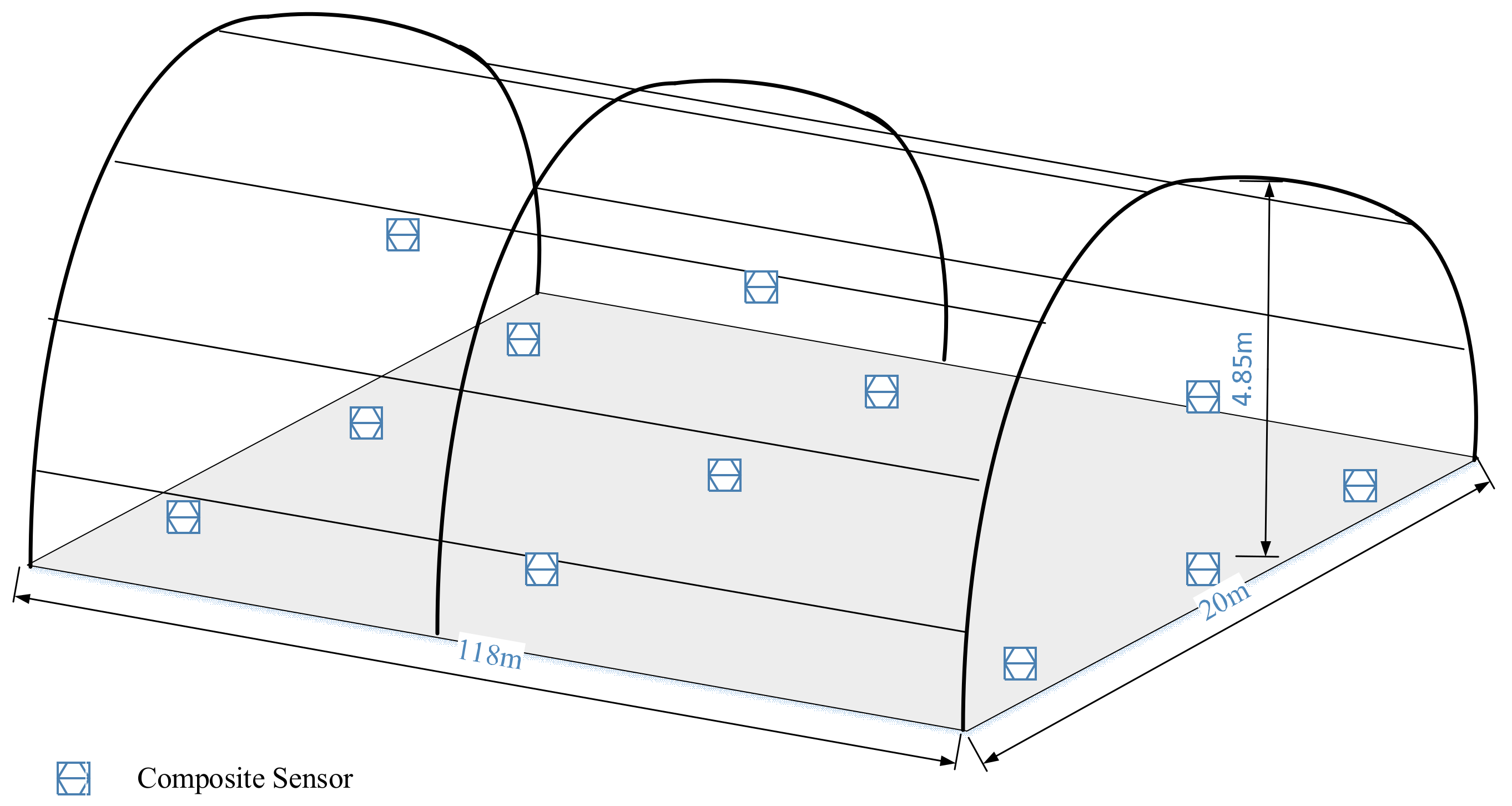
This study was conducted in the Xinjiang Kashi (Shandong Shuifa) Vegetable Industry Demonstration Garden, Kashgar, Xinjiang Uygur Autonomous Region, China (39°21′15.04″ N, 76°01′33.43″ E). The greenhouse had a dual-mode, double-arched structure (see Figure 1), with a longitudinal ridge as the greenhouse roof. The outer dimensions of the greenhouse were 118 m in length, 20 m in width, and a height of 4.85 m. The greenhouse was equipped with a quilt insulation system, a spray cooling system, and a ventilation system. We gathered data from multiple meteorological stations within the greenhouse, encompassing temperature, humidity, and solar radiation, which were critical microclimatic factors influencing crop growth in greenhouses. To ensure effective monitoring of the greenhouse environment, we strategically deployed multiple sensor arrays throughout the greenhouse and installed a miniature meteorological station for data calibration. The sensors utilized an S10A greenhouse data acquisition instrument (Green Water, NERCITA) to capture data on greenhouse temperature [°C], relative humidity [%], and solar radiation [W/m²] at a collection frequency of every 10 min. Considering data redundancy, we obtained final data at an hourly sampling rate. The entire experimental data collection spanned from 10 April to 30 August 2023.

Consistent with the frequency of data collection from small weather stations, we recorded the operational status of quilts, vents, and spraying, which also affected microclimate changes in the greenhouse. The specific recording methods were presented in

Table 1. Execution module operation records.

Implementation Module	Operational Status	Data Recording
Quilts	Quilts completely covered	0
	25% coverage by quilts	1/4
	50% coverage by quilts	1/2
	75% coverage by quilts	3/4
	Quilt completely rolled up	1
Sprayers	Turning on the sprinkler system	1
	Turning off the sprinkler system	0
Ventilation	Vent opening	1

.

We procured meteorological data for the greenhouse base during the experimental period from the Open-Meteo open-source meteorological website (https://open-meteo.com/) accessed on 1 April 2023, which included eight elements: temperature, humidity, dew point, precipitation, surface atmospheric pressure, wind direction, wind speed, and solar radiation. Owing to Open-Meteo provision of high-resolution data ranging from 1 to 11 km, which more accurately reflects extensive meteorological conditions, we calibrated our data using the external meteorological station at the experimental base.

2.2. Seedling Growth Monitoring

The greenhouses in the Vegetable Industry Demonstration Garden primarily focused on cultivating chili pepper and tomato seedlings. Sowing was carried out on 23 July 2023, with continuous documentation of seedling growth parameters across growing seasons. The materials selected were chili pepper (Hongbao No. 2) and tomato (Mao Fen 802). The experimental staff applied uniform treatments during the nursery process, including the use of plug trays, water, nutrient solutions, and substrates. We recorded the seedlings’ plant height, stem thickness, and leaf area bi-daily over the course of two months for both growing seasons.

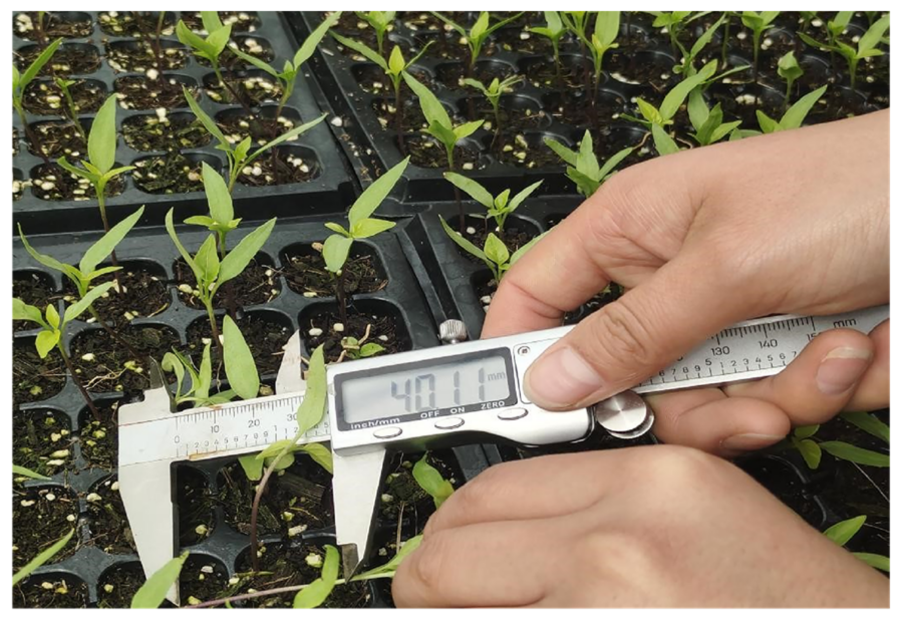
Seedling plant height was measured using a combination of IP54 electronic digital vernier calipers (150 mm, 0.01 mm) and a straightedge (200 mm, 0.1 mm) from the base of the seedling to the top of the plant, and when the plant height exceeded 150 mm, a transparent straightedge was used to estimate the plant height. For the measurement of seedling stem thickness, we used the area near the cotyledons as a marking point for the measurement, and clamped the vernier calipers gently with moderate force to measure the stem thickness (Figure 2). Considering the large error in the measurement of leaf area by the square method and the need for a large number of destructive samples by the instrumental method, together with the similarity of the size and shape rules of the two seedling leaf blades, we used vernier calipers to measure the leaf length and leaf width of the seedlings and calculated the leaf area of the seedlings according to Equation (1) [37]. We randomly sampled one hole tray for each seedling, and 18 seedlings were randomly selected from each hole tray. The data for seedling height and stem thickness were averaged, and the leaf area values for a single seedling were too small, so we summed up the leaf area records for the 18 seedlings we measured.

$$\mathrm{S}=\mathrm{L}\times \mathrm{W}\times 0.75.$$

(1)

Note: L is the blade length and W is the blade width.

Figure 2. Measurement of seedling height and stem thickness using vernier calipers.

Figure 2. Measurement of seedling height and stem thickness using vernier calipers.

2.3. Data Preprocessing

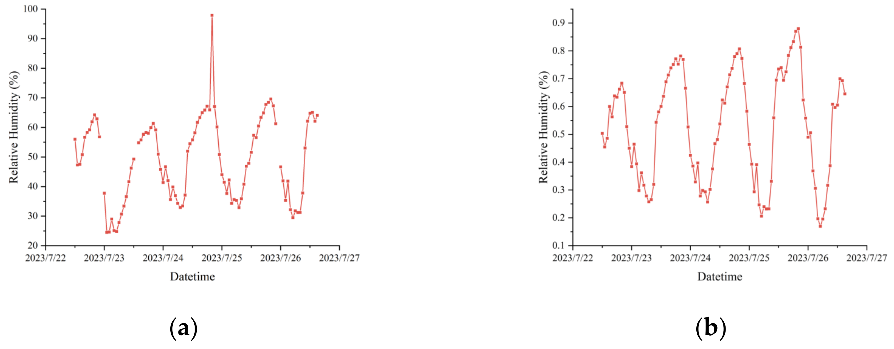
The collected data were susceptible to noise, drift, and anomalies, as illustrated in Figure 3a; therefore, quality control and data cleansing were imperative. Missing values were addressed through interpolation or deletion, and anomalies were corrected or eliminated based on domain knowledge. In this study, we employed a combination of forward filling, backward filling, and Kriging interpolation for missing value treatment, ensuring minimal introduction of noise or bias. The performance of post-missing data treatment was monitored using a single back-propagation regression model to ensure model stability and accuracy.

In multi-dimensional time series forecasting, different features may have varying levels of importance. Deep learning was highly sensitive to the scale of input data; thus, differences in scale among features can lead to instability and difficulty in model convergence. Normalization ensures that data gradients are within a reasonable range, facilitating more effective weight updates. In our research, we utilized the mapminmax function to standardize the scales of different features, thereby negating the influence of scale disparities on the predictive model. The specific computation formula was as follows [38]:

$$y=\frac{(y_{max}-y_{min}) * (x-x_{min}) }{(x_{max}-x_{min})}+y_{min} .$$

(2)

In this formula, x represented the input data sample, y was the normalized result, $y_{max}$ and $y_{min}$ were the maximum and minimum values of the target range, and $x_{max}$ and $x_{min}$ were the maximum and minimum values of the input data. In our experiments, the target range was set as [0, 1]. Data post-interpolation and normalization are depicted in Figure 3.

2.4. The Proposed Model

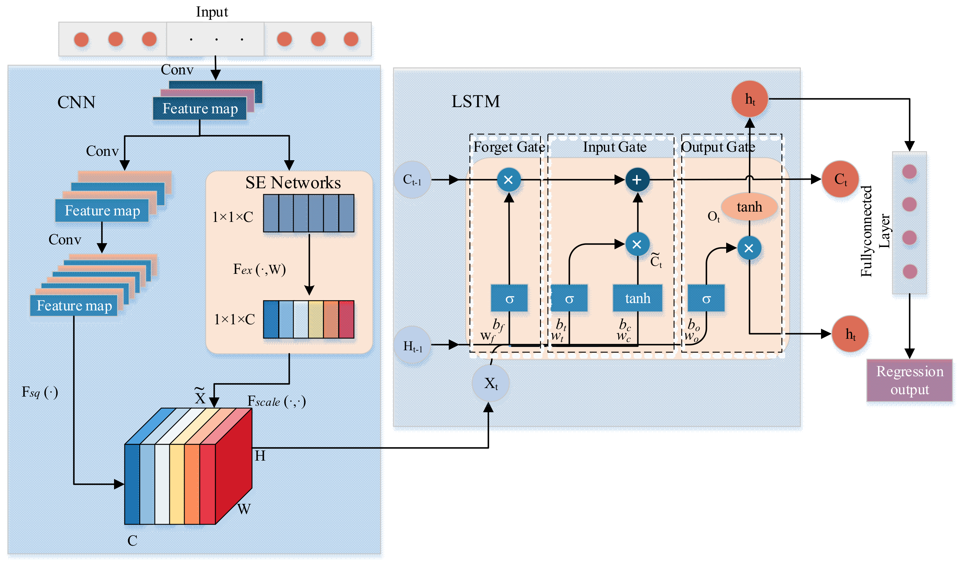
In consideration of the intricacies of the predictive task at hand, the available data, computational resources, and the performance requirements of the model, we have devised a CNN-Attention-LSTM model. As illustrated in Figure 4, for time series prediction tasks, a singular CNN model typically perceived time series data as a multi-channel matrix, with each channel representing a temporal step or feature. While the CNN model was highly adept at capturing spatial features, its ability in temporal modeling was somewhat limited due to a lack of an explicit memory mechanism for handling time dependencies. In contrast, the LSTM model, a specialized recurrent neural network designed for sequential data, exhibited robust capabilities in temporal modeling, capturing long-term dependencies within time series data. However, a standalone LSTM model may face constraints in addressing complex spatiotemporal relationships and feature extraction. Thus, our proposed model amalgamated the strengths of both CNN and LSTM, utilizing the CNN to extract spatial features, followed by the LSTM to apprehend temporal dependencies. This synergy effectively addressed the spatial and temporal characteristics inherent in time series prediction tasks. To further enhance the performance of the CNN-LSTM model, we have integrated SE Networks within the CNN segment to dynamically adjust feature weights, accentuating pivotal features. This integration not only augmented predictive performance but also imparted a degree of robustness against noise and irrelevant information.

Given the modest volume of our dataset and the constraints of our computational resources, we refrained from employing pooling layers to reduce the dimensions of feature maps. During the CNN phase, we engineered a three-layered consecutive convolutional structure to extract higher-level features, thereby enabling the model to better interpret the input data. In this research, we constructed matrices from hourly historical meteorological data and the operational status data of greenhouse mechanisms (such as quilts, ventilation, and sprinkling systems) as inputs for the CNN for foundational feature extraction. The convolutional process was delineated in Equation (3).

$$H\left(x\right)=f \otimes g={\sum }_{u=-\infty }^{+\infty }f\left(x-u\right)·g\left(u\right).$$

(3)

Note: f is the input data, g is the convolutional kernel of the CNN, and x and u are the variables in the function.

In the proposed model, the SE module was embedded in the CNN part according to the short circuit connection, and the feature map was squeezed into a 1 × 1 × C feature vector to get the global information embedding (feature vector) for each channel of U. This process was based on the global average pooling to obtain the average value of the feature map, i.e., Equation (4) [39]:

$$z_c=F_{sq}(u_c)=\frac{1}{W\times H}{\sum }_{i=1}^W{\sum }_{j=1}^H{u}_c(i,j).$$

(4)

After excitation learned the feature weights of each channel in C, the feature map with the same dimension as the squeeze operation was obtained, and the computation process was as follows [39]:

$${\mathit{s}=\mathit{F}}_{ex}\left(\mathit{z},\mathit{W}\right)=\sigma \left(\mathit{g}\left(\mathit{z},\mathit{W}\right)\right)=\sigma (\mathit{g}\left({\mathit{W}}_2\delta \left({\mathit{W}}_1\mathit{z}\right)\right)).$$

(5)

where δ denotes the ReLU activation function, and σ denotes the sigmoid activation function. ${\mathit{W}}_1$ and ${\mathit{W}}_2$ are the weight matrices of the two fully connected layers, respectively. r is the number of hidden layer nodes in the middle layer, and r is the number of hidden layer nodes in the middle layer. ${\mathit{W}}_1$ and ${\mathit{W}}_2$ are the weight matrices of the two fully connected layers, respectively. r is the number of hidden nodes in the middle layer. The compressed and activated values will be weighted by Fscale(⋅,⋅) of U to get the feature map.

In the proposed model, the LSTM segment utilized the output time series from the CNN as input. Traditional RNN often encountered issues of gradient vanishing or explosion when dealing with lengthy sequences. To address the challenges associated with long-distance memory, the LSTM incorporated a gating mechanism, significantly enhancing the data representation capabilities of the RNN. At time t, the LSTM received a feature map from the CNN output. The formula for the candidate memory cell was expressed as:

$${\tilde{C}}_t=tanh(w_c·\left[h_{t-1},x_t\right]+b_c).$$

(6)

The current state of the memory cell was given by:

$$C_t=f_t\times C_{t-1}+i_t\times {\tilde{C}}_t{C}_t=f_t\times C_{t-1}+i_t\times {\tilde{C}}_t.$$

(7)

Subsequently, the output gate value was determined as follows:

$$O_t=\sigma (w_o·\left[h_{t-1},x_t\right]+b_o).$$

(8)

Thus, the final output of the LSTM at time t was:

$$h_t=O_t\times tanh\left(C_t\right).$$

(9)

In these equations [40,41], $i_t$ and $f_t$ denote the values of the input and forget gates, respectively. The symbol σ represents the sigmoid activation function, while tanh is the hyperbolic tangent activation function. The weights and biases are represented by w and b, respectively.

We constructed the dataset by including the meteorological data of 8 elements as well as the recorded data of quilt, ventilation, and sprayer status, and the total amount of data reached 13,632 pieces; we divided the dataset according to a ratio of 8:2, i.e., 10,906 pieces were used as the training set, and 2726 pieces were used as the test set. The hardware utilized for the model construction comprised a Dell laptop, powered by an Intel(R) Core (TM) i5-8250U CPU @1.60 GHz, with 16 GB of RAM, and running on the Windows 10 operating system. The software used for model training and data processing included MATLAB 2022b V9.13.0 and Origin Pro 2021 V9.8.5.204.

2.5. Loss Function

To evaluate the discrepancy between our model predictions and actual microclimatic factors in greenhouses, we opted for the Huber loss function [42] as our loss function for model training in Equation (9). Although the Mean Squared Error (MSE) was beneficial for effective minimization of minor errors, its tendency to yield higher loss values can lead to substantial jumps during the back-propagation process, which is undesirable. While the Root Mean Squared Error (RMSE) is more sensitive to larger prediction errors, it lacks continuous differentiability, meaning its gradient cannot be directly calculated. Typically, RMSE served as an assessment metric for measuring the gap between model predictions and actual values, rather than a loss function for gradient descent optimization. The Huber loss function, commonly used in regression problems, amalgamates the properties of Mean Absolute Error (MAE) and Mean Squared Error (MSE), thus embodying characteristics of both loss functions.

$$\mathrm{L}\mathrm{o}\mathrm{s}\mathrm{s}\left(y, f\left(x\right)\right)=\left\{\begin{array}{c}\frac{1}{2}{(y-f(x\left)\right)}^2, \left|y-f\left(x\right)\right|\le \delta \\ \delta \left|y-f\left(x\right)\right|-\frac{1}{2}{\delta }^2, \left|y-f\left(x\right)\right|>\delta \end{array}\right..$$

(10)

Here, Loss(y, f(x)) represents the loss value, with y being the actual value and f(x) the model’s predicted value, and δ is the threshold parameter for the Huber loss. The Huber loss exhibits smoothness for smaller errors, aiding the stability of gradient descent algorithms.

2.6. Model Optimization Algorithm

For model parameter training, we employed the sparrow search algorithm for model optimization to minimize the loss function. Compared other optimization algorithms like Particle Swarm Optimization (PSO) or Grey Wolf Optimizer (GWO) in predicting greenhouse microclimates using CNN-LSTM models is driven by SSA unique advantages. SSA is known for its strong global search ability and higher convergence speed, making it efficient in finding optimal solutions in complex, multi-dimensional spaces [43,44]. This is crucial in the context of CNN-LSTM models where parameter space can be vast and intricate. Furthermore, SSA demonstrates superior performance in avoiding local optima compared to PSO and GWO, which is essential for ensuring the robustness and accuracy of predictive models in diverse and variable greenhouse environments. These characteristics of SSA contributed significantly to its effectiveness in optimizing neural network parameters for accurate microclimate prediction in greenhouses.

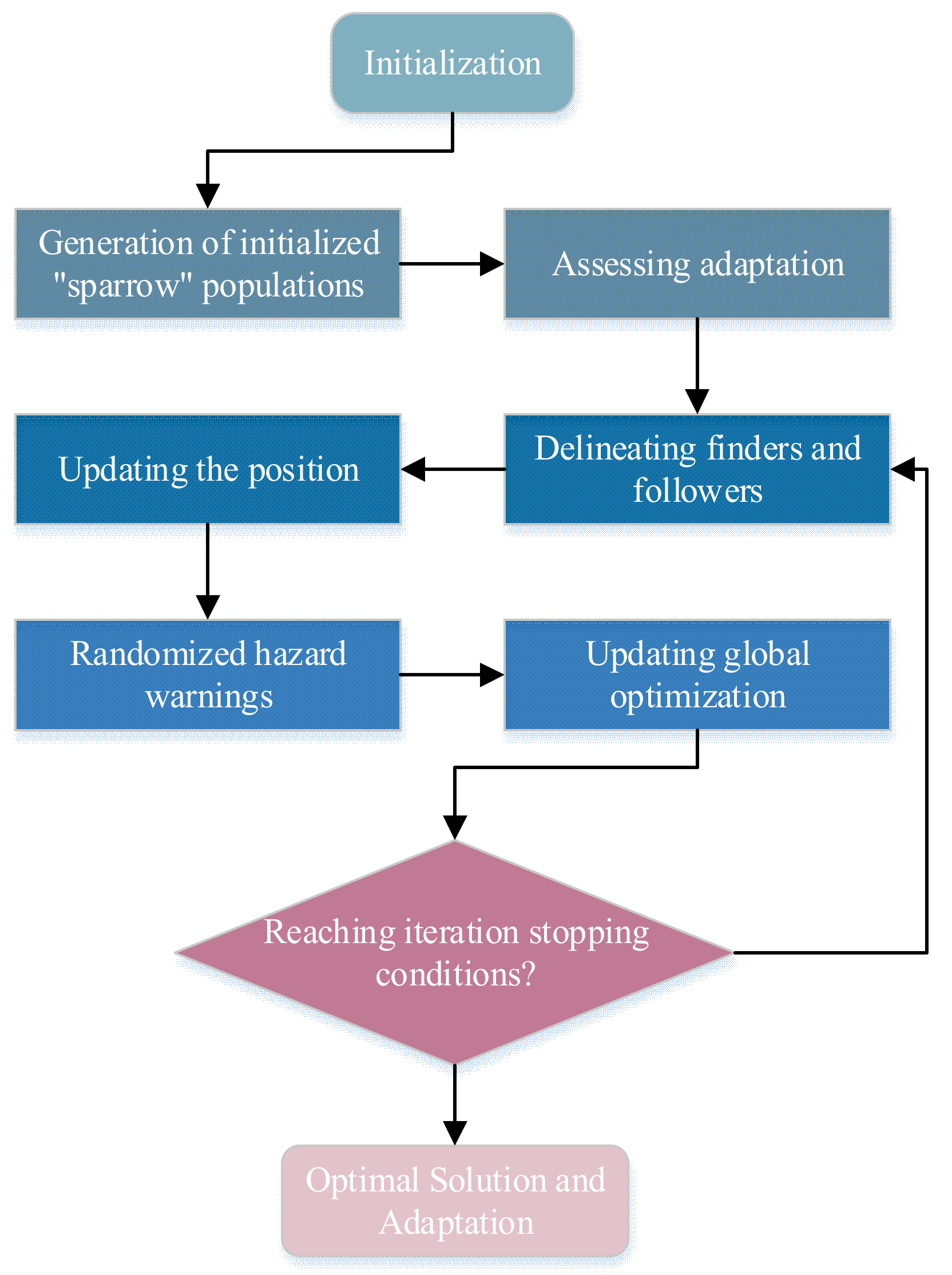
This population-based intelligence algorithm [45] abstracted the problem into an individual fitness function, progressively approximating the optimal solution through collaborative efforts within the group. Within the entire group, certain individuals acted as “discoverers” seeking food sources (termed as sparrows), while others, the “joiners”, followed the discoverers [46]. This was reflected in the algorithm as exploration (global search) and exploitation (local search) processes. When sparrows perceived a predator’s threat, they engaged in evasion, represented in the algorithm as avoiding the worst solution to prevent settling in local optima. The specific workflow was illustrated in Figure 5.

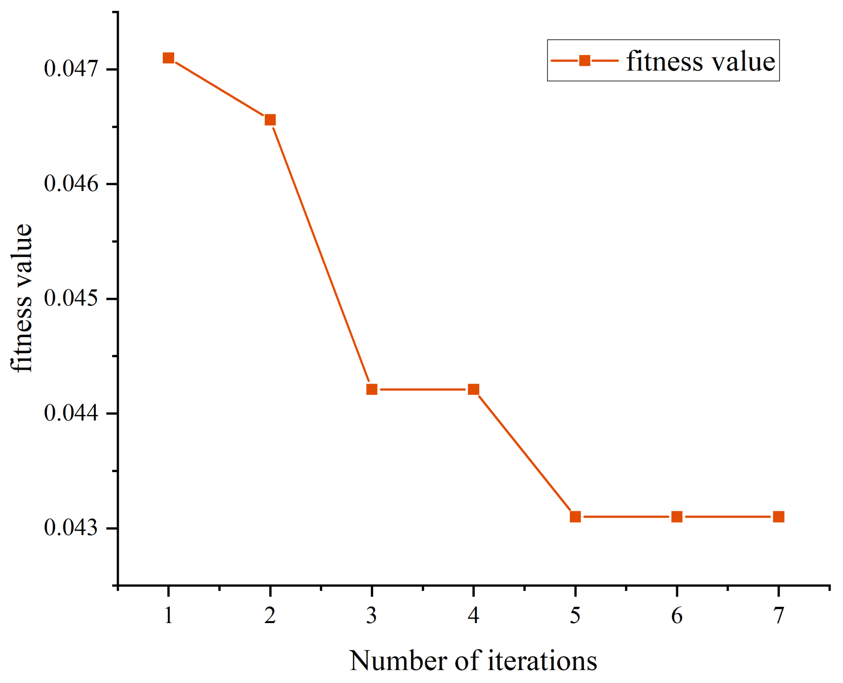
To circumvent the randomness in selecting model hyper parameters, we incorporated the SSA optimization algorithm to determine the optimal parameters for our proposed model, namely the ideal number of hidden nodes, the optimal L2 regularization coefficient, and the best learning rate. The search spaces of these three parameters are [0.01, 0.001], [10, 30], and [0.1, 0.0001]. Its fitness function was consistent with the proposed model (hybrid CNN-LSTM network combined with SE module), and the efficacy of different hyperparameter configurations is evaluated based on the performance of the training data.

In addition to using the SSA algorithm to determine the optimal learning rate, the optimal number of hidden nodes, and the optimal L2 regularization coefficients, we also needed to determine the number of training rounds and the optimizer for the model. Although increasing the number of epochs could slightly improve the model fit to training data and enhance prediction accuracy on test data, this improvement was relatively limited. It was crucial to be wary of overfitting, particularly when training for an excessive number of epochs, as the model might overlearn noise in the training data rather than underlying data distributions, potentially reducing its generalizability to new data [47]. Hence, we settled on 200 epochs as an optimal balance between model performance and computational efficiency. Since different optimizers may significantly affect the training speed, convergence, and final performance of the model, and since the CNN-LSTM we chose was a nonlinear model, we used Adam as the optimizer. The Adam optimizer combined the advantages of Adaptive gradient algorithm (Adagrad) and Root Mean Square prop (RMSprop), and was able to adaptively adjust the learning rate of each parameter, which made it more applicable in time series prediction tasks [47].

2.7. Evaluation Metrics

In this study, to comprehensively evaluate the performance of our greenhouse microclimate prediction model, we referred to the literature [48,49,50] and employed four primary evaluation metrics: Coefficient of Determination (${\mathrm{R}}^2$), Mean Absolute Error (MAE), Mean Absolute Percentage Error (MAPE), and Root Mean Squared Error (RMSE). Their computational principles are as delineated in Equations (11)–(14):

$$R^2=1-\frac{{\sum }_{i=1}^N{\left(y_i-{\widehat{y}}_i\right)}^2}{{\sum }_{i=1}^N{\left(y_i-{\overline{y}}_i\right)}^2},$$

(11)

$$MAE=\frac{1}{N}\sum _{i=1}^N\left|y_i-{\widehat{y}}_i\right|,$$

(12)

$$MAPE=\frac{100\%}{N}\sum _{i=1}^N\left|\frac{y_i-{\widehat{y}}_i}{y_i}\right|,$$

(13)

$$RMSE=\sqrt{\frac{1}{N}\sum _{i=1}^N{\left(y_i-{\widehat{y}}_i\right)}^2}.$$

(14)

In the above equations, $y_i$ represents the test value, i.e., the actual output at that moment; ${\widehat{y}}_i$ denotes the predicted value outputted by the model; N is the number of samples in the test set; and $\overline{y_i}$ represents the average of the samples.

R² measured the degree of correlation between the model predicted values and the actual values. The closer $R^2$ was to 1, the higher the accuracy of the model prediction. MAE provided an average level of prediction error and was less sensitive to outliers, offering a robust error estimate. MAPE was the average of the absolute differences between observed and predicted values as a ratio of the actual observed values, facilitating comparison across different scales. RMSE, the square root of the average of the squared differences between observed and predicted values, was suitable for scenarios where sensitivity to larger errors is paramount.

3. Results

3.1. Comparative Analysis of Hyperparameter Optimization Outcomes

To investigate the influence of model hyperparameters on the performance of our proposed model, we conducted experiments with varying parameter configurations while maintaining consistent model structure and training environments, thereby attaining optimal optimization results. Initially, we set a uniform learning rate (0.01), used the Adam optimizer, and maintained the same model structure for training sessions of 200 and 500 epochs.

Table 2. Comparison of the effect of different epochs on model performance.

Epoch	Training Set				Test Set
	${\mathbf{R}}^2$	MAE	MAPE	RMSE	${\mathbf{R}}^2$	MAE	MAPE	RMSE
200	0.984	1.651	0.035	2.203	0.884	4.198	0.081	5.527
500	0.986	1.580	0.034	2.084	0.888	4.175	0.080	5.425

shows the results of the evaluation metrics of the model (containing R2, MAE, MAPE, and RMSE) for different training epochs. The model metrics, as presented in Table 2, revealed that increasing epochs from 200 to 500 marginally enhanced the ${\mathrm{R}}^2$ value on the training set from 0.984 to 0.986, with negligible differences in MAE, MAPE, and RMSE across both training and test sets. Therefore, we set the epoch to 200, having reached the optimal balance between model performance and computational efficiency.

In examining the impact of the SSA on the performance of our proposed time series prediction model, we optimized the model using different maximum iteration configurations of the SSA algorithm for the task of predicting relative humidity in greenhouses. The results, presented in

Table 3. Prediction performance of SSA optimization algorithm with different number of iterations.

Maximum Number of Iterations	Training Set				Test Set
	${\mathbf{R}}^2$	MAE	MAPE	RMSE	${\mathbf{R}}^2$	MAE	MAPE	RMSE
5	0.909	0.755	0.028	1.098	0.707	1.945	0.083	2.587
6	0.934	1.651	0.035	2.203	0.884	4.198	0.081	5.527
7	0.967	1.195	0.043	1.225	0.951	0.936	0.068	1.618
8	0.969	2.349	0.051	3.125	0.900	3.866	0.071	5.129
9	0.967	2.424	0.053	3.214	0.897	3.925	0.076	5.192

, showed a significant increase in the ${\mathrm{R}}^2$ value on the training set from 0.909 to 0.967 when increasing the maximum iterations from five to seven, indicating a substantial improvement in the model fit to training data. The ${\mathrm{R}}^2$ value on the test set also increased notably from 0.707 to 0.951, demonstrating enhanced predictive capability for unknown data. At seven iterations, the test set showed the lowest values for MAE, MAPE, and RMSE, at 0.936, 0.068, and 1.618 respectively, suggesting optimal predictive accuracy under this parameter setting. However, increasing iterations beyond seven resulted in a slight improvement in ${\mathrm{R}}^2$ on the training set but a decrease in ${\mathrm{R}}^2$ on the test set, along with increases in MAE, MAPE, and RMSE, indicating a risk of overfitting. We determined the optimal number of iterations for the SSA algorithm based on Table 3 and plotted the fitness result curve when the maximum number of iterations was seven (Figure 6). When optimizing the hyperparameters of the prediction model using SSA again, we evaluated the prediction error by the fitness value. In Figure 6, we found that when the maximum number of iterations was seven, the fitness value reached the minimum case, i.e., the prediction error reached the minimum. This also means that the optimization process avoided falling into local optimal solutions or overfitting. Based on the above results, we thus determined the optimal LSTM hidden nodes (17), epoch (200), optimal L2 regularization coefficient (0.0001), and optimal learning rate (0.001).

3.2. Greenhouse Microclimate Prediction

We trained the model proposed in Section 2.4 to predict three elements of the greenhouse microclimate: temperature, relative humidity, and solar radiation. Focusing on relative humidity prediction as an example, Figure 7 and

Table 4. Evaluation indicators for different forecasting objectives.

Predicted Target	MAE	MAPE	RMSE	${\mathbf{R}}^2$
Temperature	0.540	0.024	0.755	0.940
Relative humidity	0.936	0.068	1.618	0.951
Solar radiation	1.586	0.203	3.417	0.936

showcased the predictive results and evaluation metrics of the proposed model. The model demonstrated high fidelity in fitting the training set data, and while its predictive performance on the test set (Figure 7) was not as robust as on the training set, the overall prediction outcomes were commendable. The small discrepancy between predicted values and actual observational data underscored the accuracy of the model predictions. We also plotted the predictive results for temperature and solar radiation (Figure 8 and Figure 9). Except for some minor deviations from actual data on specific days (solar radiation predictions for 21 and 24 August), the overall predictive outcomes were satisfactory. The evaluation metrics in Table 4 indicated an average deviation in temperature prediction of 0.54 °C, in relative humidity prediction of 0.936, and in solar radiation prediction of 1.586. The slightly higher deviations in relative humidity and solar radiation predictions were attributable to their larger scales. Overall, the proposed model demonstrated commendable generalizability.

To vividly illustrate the discrepancies between the predictive outcomes of our proposed model and the actual analytical data for microclimates in greenhouses, we had graphically represented the errors in forecasts of various elements in Figure 10, Figure 11 and Figure 12. It has been observed that the forecasted errors for the relative humidity inside the greenhouse are confined within the range of [−2, 2], with a predominant distribution in the narrower interval of [−1, 1]. Notably, the prediction errors on 20 August, 22 August, 26 August are relatively pronounced. When considering the errors in temperature and solar radiation forecasts (depicted in Figure 11 and Figure 12), the error margins were consistently stable within ±1 °C and ±2 W/m², respectively. This was particularly significant for humidity and solar radiation, where the larger scale of these variables suggested that such errors remain within an acceptable threshold.

3.3. Performance of the Predictive Model

To further substantiate the efficacy of our proposed model in predicting the microclimate of greenhouses, we conducted a comprehensive comparison between our model and other time series forecasting models, namely the Single LSTM, CNN-LSTM, CNN-SE-LSTM, and the BP neural network. This experiment was carried out under consistent experimental conditions and training parameters, with results detailed in

Table 5. Comparison of the performance of different models for multidimensional time series prediction of greenhouse microclimate.

Models	Training Set				Test Set
	${\mathbf{R}}^2$	MAE	MAPE	RMSE	${\mathbf{R}}^2$	MAE	MAPE	RMSE
LSTM	0.817	2.303	0.102	2.651	0.594	3.049	0.136	3.6577
CNN-LSTM	0.859	0.898	0.034	1.273	0.729	2.259	0.095	3.06
CNN-SE-LSTM	0.913	0.862	0.032	1.23	0.796	1.213	0.093	3.007
BP-Network	0.715	3.302	0.101	3.651	0.684	4.049	0.136	4.658
Proposed model	0.967	1.195	0.043	1.225	0.951	0.936	0.068	1.618

.

Overall, the Single LSTM model exhibited suboptimal performance on the training dataset, with an ${\mathrm{R}}^2$ score of 0.817. This score suggested a moderate degree of fit to the training data. Its performance was even more lackluster on the test dataset, with an ${\mathrm{R}}^2$ of merely 0.594, accompanied by relatively higher Mean Absolute Error (MAE) and Root Mean Square Error (RMSE) values, indicating limited predictive capability for unfamiliar data. In contrast, the CNN-LSTM model showed improved performance on both training and test datasets, underscoring the enhanced learning capability brought about by the integration of CNN. The BP network model fared the worst among the models, both on the training and test datasets.

Of all the models evaluated, our proposed model demonstrated superior performance in predicting the microclimate of greenhouses. It achieved an impressive ${\mathrm{R}}^2$ of 0.967 on the training dataset and 0.951 on the test dataset, significantly outperforming the other models. Additionally, it exhibited the best results in terms of MAE, MAPE, and RMSE, indicating its excellent fit and generalization capabilities. Although the CNN-SE-LSTM also displayed commendable performance, particularly in terms of generalization on the test dataset, this further elucidates the potential of the SSA algorithm in enhancing model predictive performance.

3.4. Impact of the Proposed Model on Greenhouse Seedlings

To rigorously assess the practical utility of our proposed model, we applied it to the autumn nursery cultivation. The model enabled us to regulate the greenhouse environment—temperature, relative humidity, and solar radiation—by adjusting ventilation, quilts, and sprayer, thereby maintaining conditions conducive to seedling growth. Concurrently, we conducted identical experiments in a neighboring greenhouse (without the utilization of the proposed model for management), ensuring consistency in seedling varieties and nutritional conditions. The results are presented in

Table 6. Growth parameters of Autumn seedlings without the proposed model.

Days of Cultivation	Chili Pepper Seedling			Tomato Seedlings
	Plant Height	Stem Thickness	Leaf Area	Plant Height	Stem Thickness	Leaf Area
5	5.26	0.7	11.07	6.22	0.75	28.62
10	9.01	1.01	21.29	11.75	1.21	47.23
15	16.15	1.28	43.84	17.68	1.76	90.85
20	22.69	1.91	68.45	26.93	2.02	128.47
25	37.23	2.05	126.13	36.55	2.49	199.02

and

Table 7. Growth parameters of Autumn seedlings with the proposed model.

Days of Cultivation	Chili Pepper Seedlings			Tomato Seedlings
	Plant Height	Stem Thickness	Leaf Area	Plant Height	Stem Thickness	Leaf Area
5	13.96	1.02	39.61	11.53	1.16	93.39
10	35.84	1.97	100.18	37.06	2.12	141.89
15	46.87	2.96	176.14	62.68	2.89	279.16
20	70.98	3.25	258.46	74.64	3.55	387.4
25	81.73	4.12	290.44	98.6	5.09	428.44

.

Our findings, as detailed in these tables, reveal that irrespective of the model application, all parameters (plant height, stem thickness, and leaf area) exhibited growth correlating with the duration of cultivation. Significant growth was observed in both chili pepper and tomato seedlings in terms of plant height, stem thickness, and leaf area. For instance, on day 25, chili pepper seedlings cultivated with the model showed measurements of 81.73 mm in height, 4.12 mm in stem thickness, and 290.44 cm² in leaf area, compared to 37.23 mm, 2.05 mm, and 126.13 cm², respectively, for those cultivated without the model. The growth curves of seedlings, pre- and post-model application, are visually depicted in Figure 13. Overall, chili and tomato seedlings grown with the model demonstrated noticeably faster growth rates in plant height, stem thickness, and leaf area within 25 days than those grown without it. To further statistically analyze the model’s differential impact on the growth parameters of chili and tomato seedlings, we conducted independent sample T-tests, with results depicted in

Table 8. Results of T-test analysis of seedling growth parameters.

Seedlings	Growth Parameters	T-Statistics	p-Value
chili pepper seedlings	Plant height	−2.37	0.045
	Stem thickness	−2.14	0.065
	Leaf area	−2.32	0.049
Tomato seedlings	Plant height	−2.32	0.049
	Stem thickness	−1.80	0.110
	Leaf area	−2.31	0.050

. Except for stem thickness, the p-values for plant height and leaf area in both chili and tomato seedlings were less than 0.05, indicating significant differences between model usage and non-usage in these aspects. This variance underscored the efficacy of the CNN-LSTM model in accurately predicting and regulating microclimatic conditions within the greenhouse, thereby optimizing the plant growth environment and enhancing crop growth rate and biomass.

4. Discussion

Greenhouses, as complex, time-variant systems, were characterized by an intricate interplay of various environmental factors [51]. Additionally, the nature of crops grown within the greenhouse also dictated the extent of interaction among these environmental variables, leading to differing levels of system stability in response to environmental changes [52,53,54]. Consequently, predictions based solely on single variables fell short of establishing an accurate microclimatic forecasting system for greenhouses. This study aimed to establish a time series prediction model for the greenhouse microclimate, using multi-feature meteorological data and greenhouse control system statuses, to accurately predict future temperature, relative humidity, and solar radiation in greenhouses. We integrated CNN and LSTM to build and optimize a greenhouse microclimate prediction model and used it to adjust the suitability of the greenhouse seeding environment. Our contributions include: (1) Exploring a deep learning architecture that combined CNN and LSTM for time series prediction of greenhouse microclimates; (2) proposing a model embedding SE Networks for feature recalibration to enhance model predictive performance; (3) introducing the SSA for parameter optimization of the model, further improving predictive accuracy; and (4) validating the effectiveness of the model in greenhouse seedling cultivation. The accurate prediction of the greenhouse microclimate allowed for precise adjustment of the seedling environment, thereby significantly improving both the efficiency of seedling cultivation and the quality of plant growth.

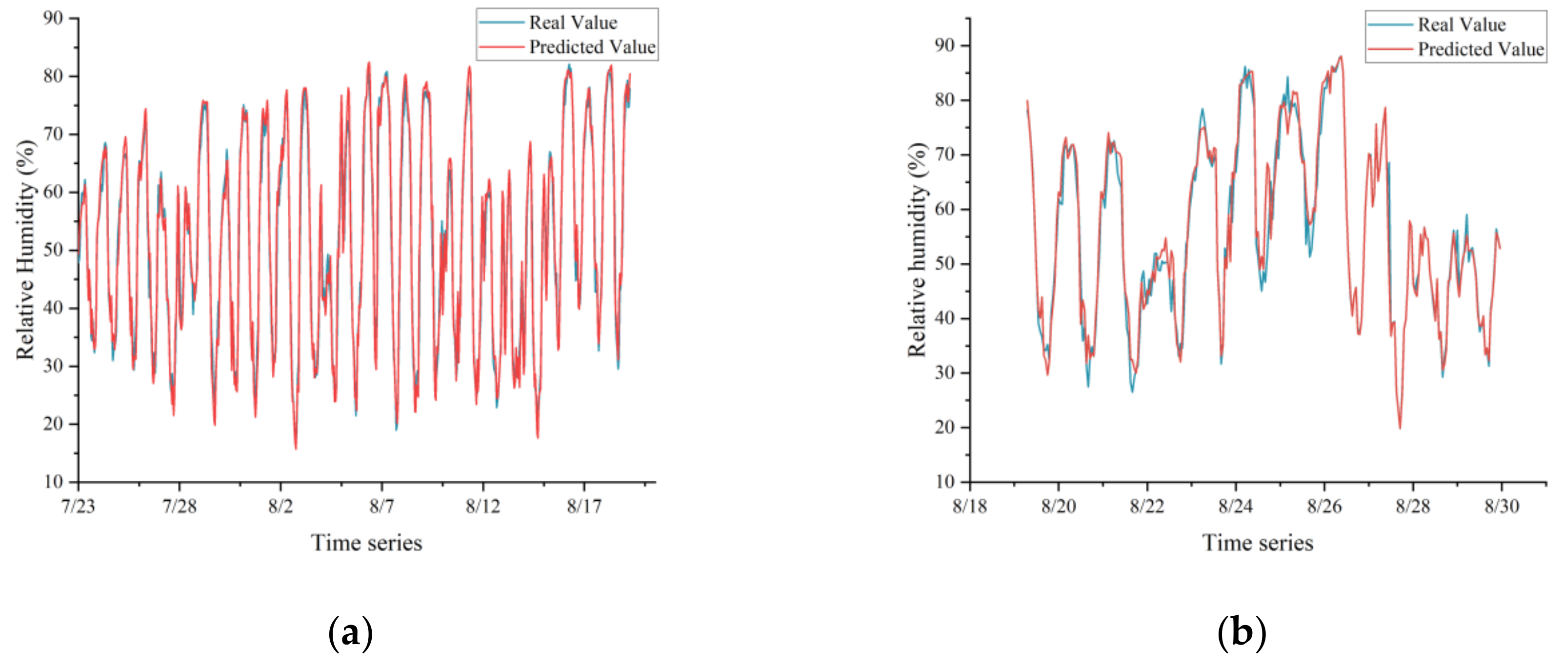
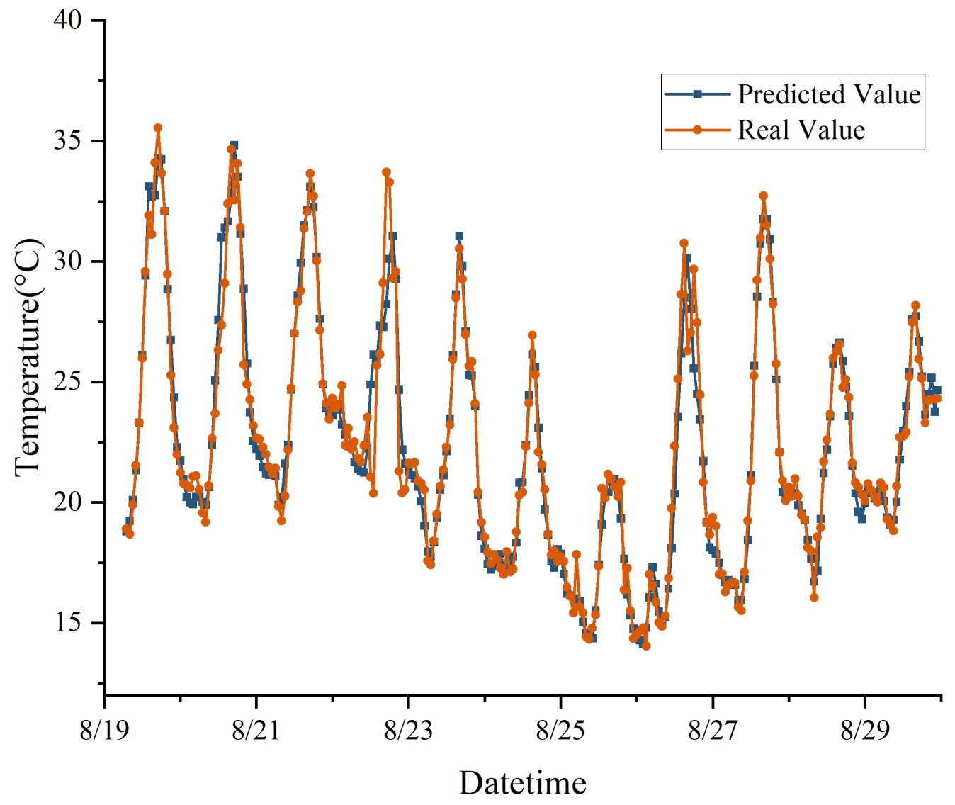
In this study, a model combining CNN and LSTM networks was proposed, demonstrating exceptional proficiency in analyzing complex spatiotemporal dynamics within greenhouse environments to predict microclimates. Notably, the model achieved impressive R² and RMSE values, signifying its high accuracy in forecasting relative humidity. The integration of CNN and LSTM leveraged their respective strengths in spatial feature extraction and time-dependent modeling, crucial for microclimate prediction. Additionally, the application of SE networks and SSA further enhanced the model’s performance, particularly in generalization on test sets, although the model without SSA optimization showed slightly lower performance metrics. Comparatively, this research aligned with and extends previous studies, such as Jung et al. [13] and their LSTM-based models for evapotranspiration and humidity in tomato greenhouses, and Xie et al. [22] and their application of an enhanced Grey Wolf Optimization algorithm for optimizing CNNs and LSTMs. It also resonated with findings from a study predicting solar greenhouse and crop water demand using LSTM and CNN-LSTM models [34]. Furthermore, the work of Esparza et al. [55] using LSTM-RNN and XGBoost for temperature forecasting in greenhouses corroborated the effectiveness of integrating various modeling approaches, as observed in our study. These comparisons underscored the advanced capabilities of LSTM-based models in precise time series prediction within agricultural contexts.

In terms of hyperparameter optimization, we discovered that increasing the number of epochs can enhance model performance, albeit with diminishing returns and the risk of overfitting. Consequently, we selected 200 epochs as the termination condition for model training, balancing performance, and computational efficiency. The SSA optimization algorithm excelled in determining the optimal number of hidden nodes, L2 regularization coefficients, and learning rates, further validating its potential in optimizing deep learning models. 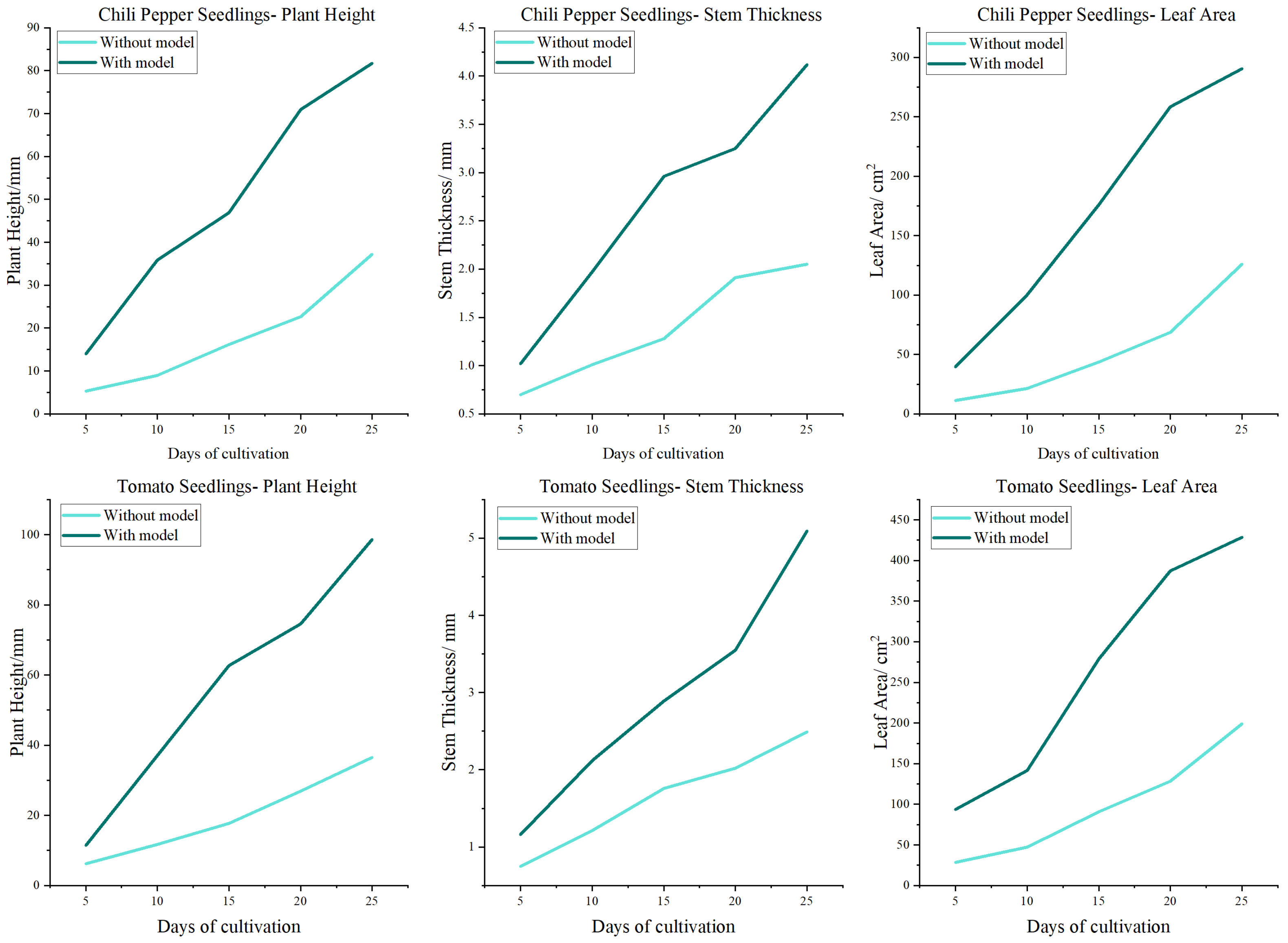Further, as discerned from Table 6 and Table 7, employing the proposed model to predict and accordingly adjust the microclimate within greenhouses during the autumn significantly enhanced the growth of chili pepper and tomato seedlings. In contrast, the data from the seedling cultivation, which did not utilize the model, indicated a slower rate of plant growth, particularly in terms of leaf area expansion. This comparison underscored the profound impact of applying deep learning models in optimizing plant growth conditions, thereby augmenting both the pace and quality of crop development. This aligned with the findings of Li et al. [16], who reported that the application of deep learning models can optimize plant growth conditions, thereby enhancing crop yield and quality.

While the study’s use of data from Kashgar, Xinjiang’s Vegetable Industry Demonstration Garden yielded positive results, it faced limitations in dataset diversity and model predictive accuracy. The dataset, though extensive, may not fully capture the variance across different greenhouse environments. Future work should include a broader range of data, encompassing various geographic locations, greenhouse types, and crops. Additionally, improvements were needed in predicting solar radiation, potentially by integrating more comprehensive meteorological data, such as cloud cover and soil conditions. The study’s use of the sparrow search algorithm (SSA) proved effective in optimizing model parameters but was computationally intensive, suggesting a need for more efficient algorithms in future research to better suit large-scale or real-time applications.

5. Conclusions

In this work, we designed and investigated a greenhouse microclimate prediction model based on integrating CNN and LSTM networks and used it to optimize the environmental suitability of greenhouse seedlings. The main conclusions are as follows:

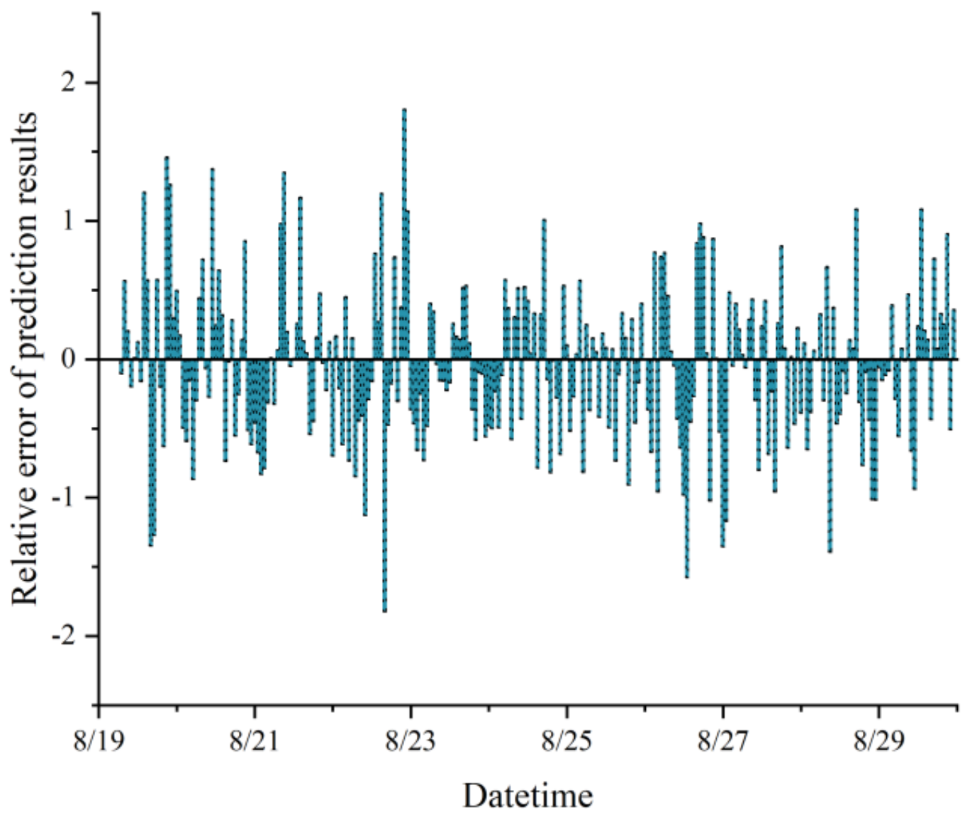
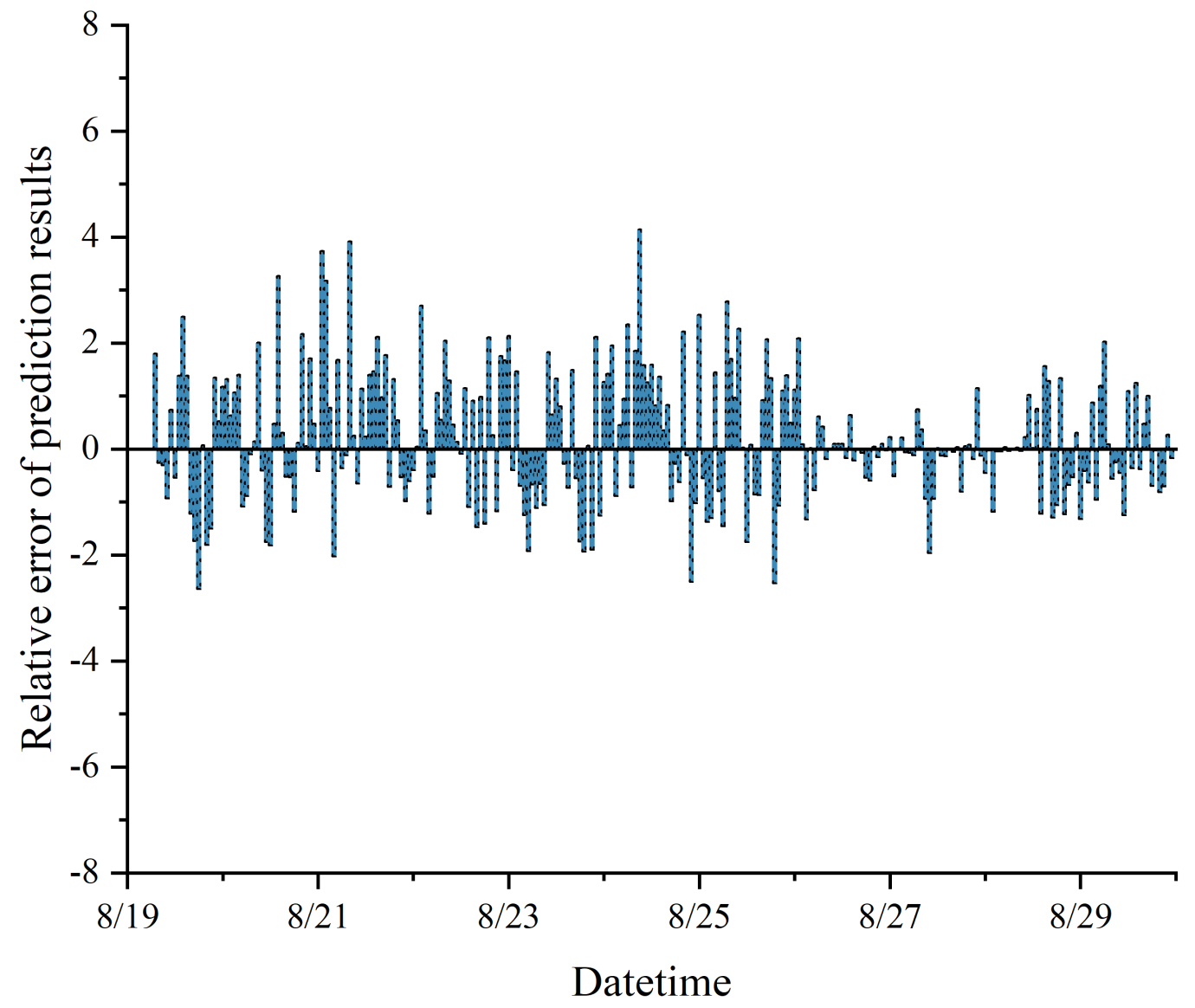
• In this study, we successfully constructed a greenhouse microclimate prediction model by integrating CNN, SE network, and LSTM, and realized a more accurate prediction effect, with prediction errors of 0.540 °C, 0.936%, and 1.586 W/m² for temperature, humidity, and solar radiation, respectively.
• The sparrow search algorithm effectively optimizes the model parameters and determines the best configuration scheme with a learning rate of 0.001, an L2 regularization parameter of 0.0001, and 17 hidden units, which further improves the prediction accuracy of the model.
• The model’s success in precisely regulating greenhouse conditions provides new solutions for further research into environmental control and crop yield optimization, particularly in the context of climate change.
• Our proposed prediction model was applied to greenhouses to optimize the suitability of nursery environments and effectively improved greenhouse nursery efficiency and seedling quality.

In summary, our proposed prediction model based on deep learning achieves satisfactory results in greenhouse microclimate prediction and optimizing the environmental suitability of greenhouse seedlings. However, this work still has limitations: despite the comprehensiveness of the dataset, it may not fully encompass the variability of different greenhouse environments. Solar radiation prediction, in particular, could benefit from the inclusion of more diverse meteorological data. Future research should focus on diversifying data sources to include a wider range of geographic locations, greenhouse types and crops. We favor the integration of more complex meteorological factors, such as cloud cover and soil conditions, to refine solar radiation predictions. Last but not least, exploring more computationally efficient algorithms could improve the applicability of models in large-scale or real-time agricultural scenarios.