Article

Time Series from Sentinel-2 for Organic Durum Wheat Yield Prediction Using Functional Data Analysis and Deep Learning

by
Adriano Mancini
1,
Francesco Solfanelli
2,*,
Luca Coviello
3,
Francesco Maria Martini
2,
Serena Mandolesi
4 and
Raffaele Zanoli
2
1
Dipartimento di Ingegneria Dell’Informazione (DII), Università Politecnica Delle Marche, Via Brecce Bianche 12, 60131 Ancona, Italy
2
Department of Agricultural, Food and Environmental Sciences (D3A), Università Politecnica delle Marche, Via Brecce Bianche 10, 60131 Ancona, Italy
3
Università di Trento, Via Sommarive 5, 38123 Trento, Italy
4
Dipartimento di Scienze e Ingegneria della Materia, dell’Ambiente ed Urbanistica (SIMAU), Università Politecnica delle Marche 12, Via Brecce Bianche, 60131 Ancona, Italy
*
Author to whom correspondence should be addressed.
Agronomy 2024, 14(1), 109; https://doi.org/10.3390/agronomy14010109
Submission received: 4 December 2023 / Revised: 22 December 2023 / Accepted: 27 December 2023 / Published: 1 January 2024

Abstract

:
Yield prediction is a crucial activity in scheduling agronomic operations and in informing the management and financial decisions of a wide range of stakeholders of the organic durum wheat supply chain. This research aims to develop a yield forecasting system by combining vegetation index time-series data from Sentinel-2 L2A time-series data, field-measured yields, and deep learning techniques. Remotely sensed data over a season could be, in general, noisy and characterized by a variable density due to weather conditions. This problem was mitigated using Functional Principal Component Analysis (FPCA). We obtained a functional representation of acquired data, and starting from this, we tried to apply deep learning to predict the crop yield. We used a Convolutional Neural Network (CNN) approach, starting from images that embed temporal and spectral dimensions. This representation does not require one to a priori select a vegetation index that, typically, is task-dependent. The results have been also compared with classical approaches as Partial Least Squares (PLS) on the main reference vegetation indexes such as the Normalized Difference Vegetation Index (NDVI) and Normalized Difference Red Edge index (NDRE), considering both in-season and end-season scenarios. The obtained results show that the image-based representation of multi-spectral time series could be an effective method to estimate the yield, also, in the middle stage of cropping with R2 values greater than 0.83. The developed model could be used to estimate yield the neighbor fields characterized by similar setups in terms of the crop, variety, soil, and, of course, management.

1. Introduction

Durum wheat food products, such as bread, pasta, and semolina, play an essential role in the Italian organic market [1,2]. However, durum wheat availability is strongly dependent on imports due to a consistent gap between domestic production and consumption [3]. The dependence on imports is exposing both the organic and conventional supply chains to several economic and financial challenges, mainly related to the phenomena of the volatility of international prices and uncertainty of supply [4,5]. Given the strategic importance of organic durum wheat products, updates and reliable data on crop yield are essential for sound decision making along the whole supply chain [6,7,8,9].
Yield prediction, which is the estimation of the crop field production over space and time, is a crucial activity in scheduling agronomic operations like decisions on the type and quantity of fertilization and irrigation and the identification of less productive field plots [10,11,12,13,14,15,16]. In organic farming systems, where crops are usually subject to more agronomic drawbacks, the adoption of precision farming through timely yield prediction could help in the reduction of the yield gap between conventional and organic crop production [17,18].
Accurately predicting crop yields is central not only for optimizing management practices [12,14] but also for informing the management and financial decisions of a wide range of stakeholders [19,20]. At the supply-chain level, crop yield prediction can help make decisions on crop distribution and the price structure and forecast potential fluctuations in import and export prices [20]. Crop yield prediction can be a useful element in crop insurance programs to effectively estimate potential yield losses and compute the relative premium rate paid to farmers [7,21,22]. In organic certification systems, yield estimates can assist the control bodies in the detection of potential fraud, as the use of forbidden inputs (e.g., fertilizers and pesticides) during the production process occurs with the purpose of increasing yield.
Yield forecast analysis is an essential element on which to base decisions for farmers’ organizations and policymakers at national and international levels as it can contribute to making analysis useful for planning and implementing proper policy initiatives [7,21,22]. In countries where the volatility of international prices could expose the populations to economic and social challenges, mainly due to the strong dependence on the imports of some crops (e.g., wheat in Mediterranean countries), yield forecasting analysis is of primary importance for farmers’ economies and global food security [4,5,6,15].
Innovative approaches are needed to improve the collection, quality, and availability of crop yield data at all stages of the supply chain. The actual climate change underlines how yield estimation is heavily dependent on several factors such as temperature, humidity, pH, rainfall, vegetation indexes, pollen data, and others that need the help of remotely sensed data and big data analysis to allow the best profitability [6,23].
In a rapidly changing world, integrated platforms based on satellite technology, sensors, digital mapping, ecological modeling, and connectivity need to be incorporated with agronomic science to monitor, assess, and manage cropland areas and to improve yield prediction [6,10,12,13,21,24,25,26,27,28,29,30,31,32,33]. Remotely sensed data allow monitoring with a proper spatial-, spectral-, and temporal-resolution crop over a season [11,33]. The use of satellite-based observations to monitor crop yield can guide the application of precision farming with a higher temporal resolution (1–5 days) and a broader coverage with a typical Ground Sampling Distance (GSD) [15,22,34]. More specifically, the availability of Sentinel-1 and Sentinel-2 data has changed, in a meaningful way, monitoring [15,35].
Using models based on high-temporal-resolution data can contribute to estimating yields and mapping the variability inside a field precisely since satellite images can help interpret crop vitality, soil properties, and climate stress [36]. Another advantage to using satellite data is the possibility to gain vegetation phenological information continuously at local to global scales [36]. On the other hand, data could be influenced by clouds and shadows, which affect the quality of information and may negatively impact the estimation [11].
A time-series approach based on remotely sensed vegetation index (VI) time-series data opened new ways for this kind of analysis [22,35]. The importance of using VI time series generally refers to the information they provide about cropping phenology patterns [36]. Furthermore, recent progress on artificial intelligence has opened new ways to improve the yield estimation from remotely sensed data. Traditional machine learning approaches are integrated by deep learning and temporal convolutional networks (TCNs) that outperform the classical machine learning method (e.g., neural network, random forest) and have been successfully applied [37].
The crop yield prediction using machine learning is a topic that received, over the past years, a lot of attention considering that this kind of information provides decisional support to farmers and agronomists [38].
Deep learning, a subset of artificial intelligence, has revolutionized the estimation of crop yields, offering numerous benefits to the agricultural sector. Its primary advantage lies in its ability to process and analyze vast amounts of data from diverse sources such as satellite imagery, weather patterns, and soil conditions [39]. Most of the existing approaches relies on historical data for the yield. The availability of time-series data for yields that are also augmented with imagery, weather, and soil data is the most complete setup, but it sets a hard requirement. In some areas, it is not feasible to acquire all these data considering the costs, and in many cases, the yield data are linked to the field or a portion of it. This could be reasonable for a district/regional analysis [40]. From the analysis of the state of the art, the widely used approaches rely on Long Short-Term Memory (LSTM) and Convolutional Neural Network (CNN) approaches. It should be considered that crop yield prediction is a complex problem due to the interaction of several factors such as crop area, temperature, light intensity, rainfall (also considering intensity), and management, and local models are needed to mimic a crop’s dynamics. LSTM approaches have also been extended using Bidirectional LSTM (Bi-LSTM), considering that they can process data in both forward and backward directions, essentially looking at sequences from both ends; this has been used for this kind of task, as in [41]. A novel variant of LSTM is the Gated Recurrent Unit (GRU). GRUs are similar to LSTMs but come with a simpler structure, combining the forget and input gates into a single update gate. Like LSTMs, GRUs can model time-series data effectively but are computationally more efficient [13]. The above-mentioned approaches overtake the well-known limits of the classical Recurrent Neural Networks (RNNs) that suffer from the matter of vanishing gradients.
In this paper, starting from remotely sensed time series, we try to estimate the crop yield using CNN models that have been adapted to manage, as input, images that embed temporal and spectral information. The work focuses on organic durum wheat yield by combining vegetation index time-series data, field-measured yield data, and deep learning techniques. Starting from Sentinel-2 L2A time-series data, the analysis focuses on the estimation of durum wheat yield considering two different approaches. The first implements Functional Principal Component Analysis (FPCA) on the vegetation index time series [42,43] that have been processed using a Partial Least Square (PLS) approach to have a baseline using a lower number of predictors. The second approach uses an image-based approach to generate images that embed both temporal and spectral domains. We decided to consider CNNs to capture, as much as possible, the temporal–spectral patterns; different models have been evaluated over different temporal windows considering in-season and end-season scenarios. The developed models are useful to predict the yield in neighbor fields that have same crop variety with a similar soil configuration, which is a typical scenario in several districts.
The paper is structured as follows. The Section 2 describes the methodological approach and the data collection procedure. The results of the different approaches used to make yield estimates are provided in Section 3. Within the Section 4, factors influencing the accuracy of both the crop yield distribution map and the regression models used for yield estimates are discussed. The paper ends with some concluding remarks.

2. Materials and Methods

In this section, we introduce the materials and methods of this work. First, we introduce the workflow, and then we present the dataset and the related algorithms and methodological approaches we adopted.

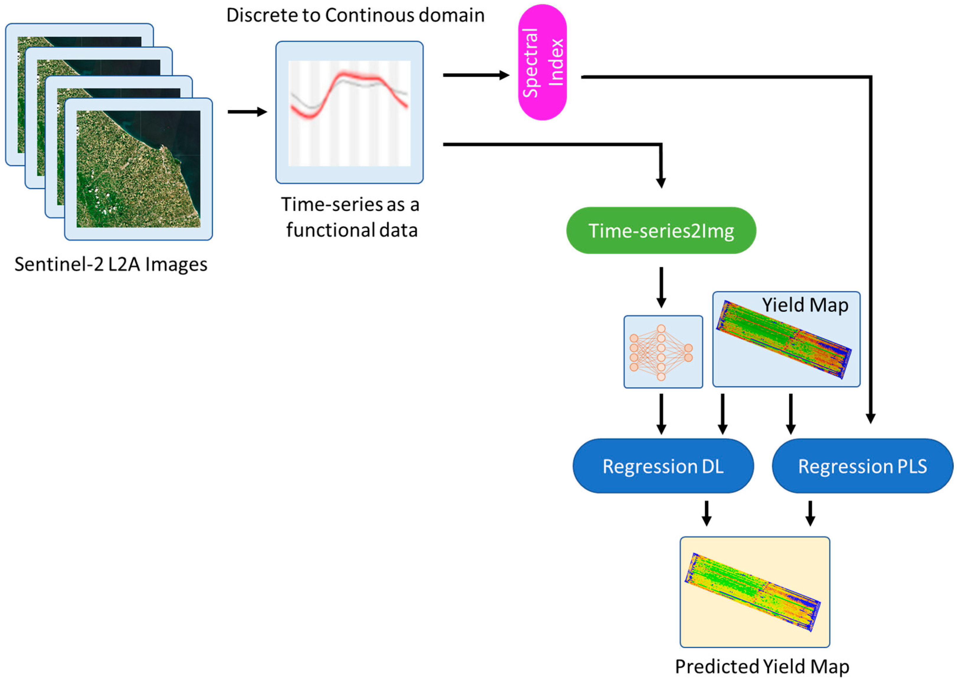
2.1. Workflow in Brief

In this sub-section, we introduce the workflow we adopted to process the remotely sensed time series. Figure 1 shows the pipeline we implemented. The first task is the downloading of data. In our case, we decided to use Sentinel-2 L2A, considering that this kind of data has a good compromise between temporal, spatial, and spectral resolutions and that it is also open. We used the Scene Classification Map (SCM) to filter out useless pixels as in the case of shadows and clouds. The time series was built for each pixel of the area of interest. We transformed time series into continuous functions, representing the spectral temporal variations, using Generalized Additive Models (GAMs), and then, using Functional Principal Component Analysis, we generated new curves of Normalized Difference Vegetation Index (NDVI) and Normalized Difference Red Edge (NDRE).
We derived two streams. The first stream focuses on a PLS regression task over different temporal windows to perform yield prediction.
The second stream tries to exploit all the available bands over different temporal windows; for each pixel, an image that embeds both time and spectral domains is generated. These images are then used to train a model that tries to perform a forecast on the final yield. In this way, we created a new domain to represent time series, enabling convolutional neural networks to capture, as much as possible, behavior over time and across spectra.

2.2. Study Area and Field Measurement

The field experiment was conducted in three different field plots located in a lowland area of central Italy in 2017 crop season. The area is characterized by a Mediterranean climate, with dry summers and rainfall (about 770 mm) concentrated in autumn and winter. The mean annal temperature is about 15 °C. The reference crop was durum wheat, cultivated on a total surface of 50 hectares over the reference fields. Using harvesting methods, yield data were collected, mapping dry and wet weight with a combine header of 7.6 m (see Figure 2).
An important aspect that could have impacted the accuracy of the regression models comprised crop yield data and the alignment of data with the GSD of the Sentinel-2 images. The width of exported yield data (i.e., 7.6 m) and the different GSD of each band (e.g., 10, 20 m) were not aligned, and this affected the relation between time series and final yield. The local variability of a pixel, considering the 8 connected ones, could have been influenced by the acquisition process (e.g., tractor’s speed).
Sentinel-2 L2A images were collected using the Sentinel-hub API from https://www.sentinel-hub.com/develop/api/ (accessed on 6 November 2023), and we considered the following bands: B01, B02, B03, B04, B05, B06, B07, B08, B8A, B09, B11, and B12. A total of 57 images from the reference period (from seeding (16 November) to harvest (17 July)) were selected.
We excluded images with clouds within the areas of interest. The images were pre-processed using the SCM to exclude pixels with “anomalous” values. A spatial resolution of 10 m was utilized, with the bands at 20 m or more resampled using the nearest-neighbor approach. Each acquisition date was also converted into day and week numbers. The first acquisition date represents the reference time to derive the numbers of days and weeks for all the images in our archive. Based on previous literature [43], we decided to post-process each time series by interpolating and smoothing it using GAM. Figure 3 shows an example of GAM interpolation considering the NDVI index in the study area.

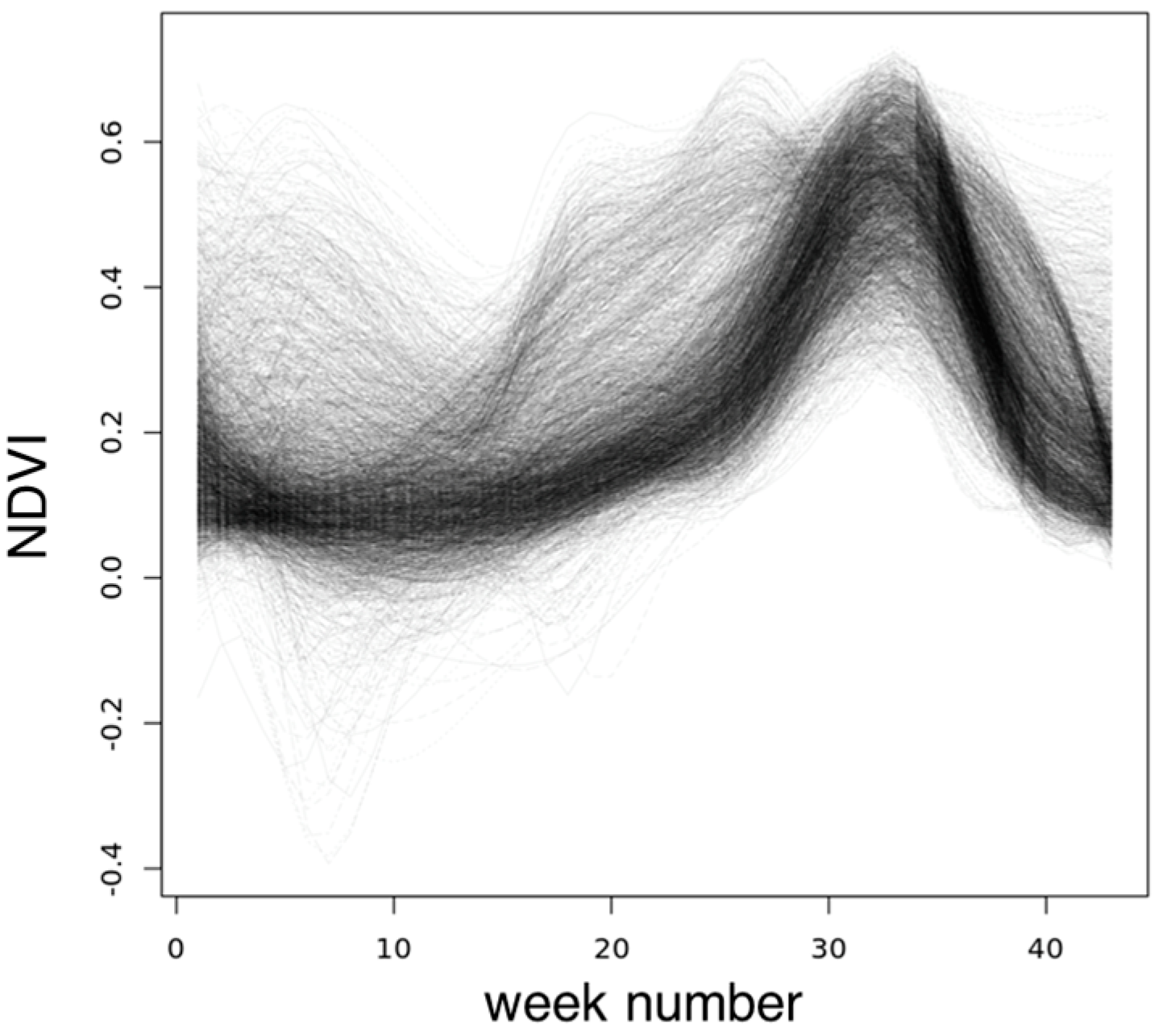
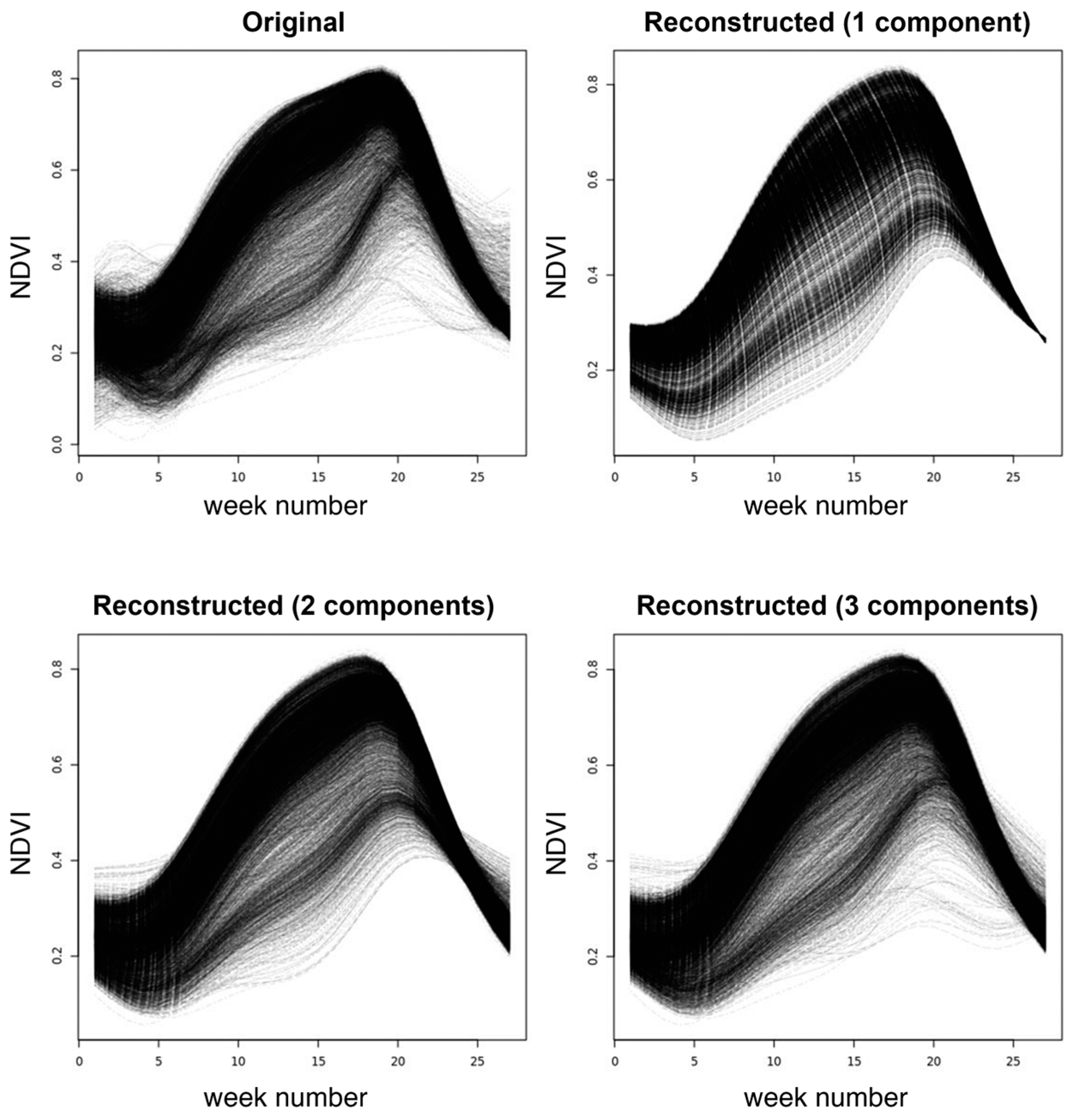
2.3. Funcional Data Analysis

FPCA is a statistical technique used to analyze and extract the underlying patterns in functional data [44,45]. It is particularly useful when working with data that consist of curves or functions, such as time series, growth curves, or spectral data. FPCA extends the traditional Principal Component Analysis (PCA) to handle functional data, allowing for a more comprehensive analysis of the variation and structure within the data. In FPCA, the data are represented as a set of continuous functions. These functions can be seen as smooth curves that vary over some continuous domain, such as time or space. The goal of FPCA is to find a small number of principal components that capture most of the variability in the data, similar to PCA in multivariate analysis. The key idea behind FPCA is to decompose the functional data into a sum of orthogonal functions known as eigenfunctions. These eigenfunctions are obtained by solving an eigenvalue problem, wherein the eigenfunctions represent the directions in the function space that explain the most variation in the data. The eigenfunctions are ordered according to their corresponding eigenvalues, with higher eigenvalues indicating greater variability explained. These eigenfunctions represent the functional principal components (FPCs) and provide a low-dimensional representation of the data. The FPCs obtained from FPCA can be interpreted as smooth functions that capture the dominant modes of variation in the data. The first few FPCs often explain a large proportion of the total variation, allowing for dimension reduction and “simplification” of the data. In our case, we decided to reconstruct the time series by using the number of components that ensured that over than the 90% of the variance was explained [43]. Figure 4 shows the effect of the number of components on the reconstructed functions.

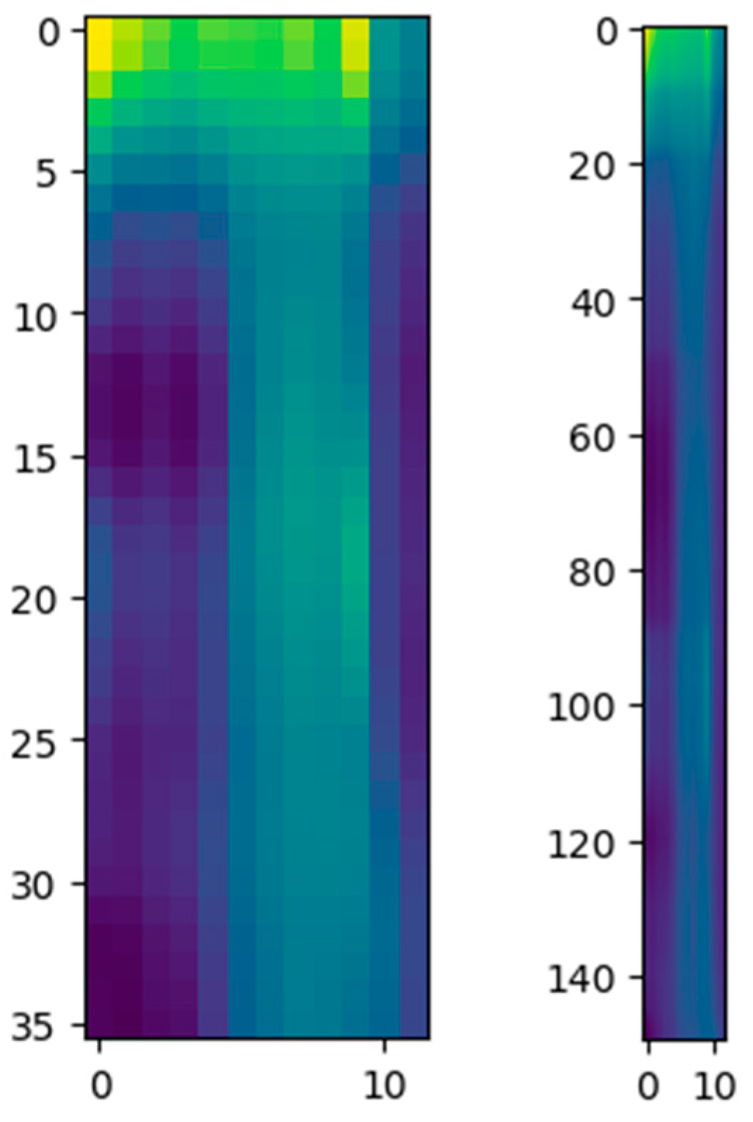
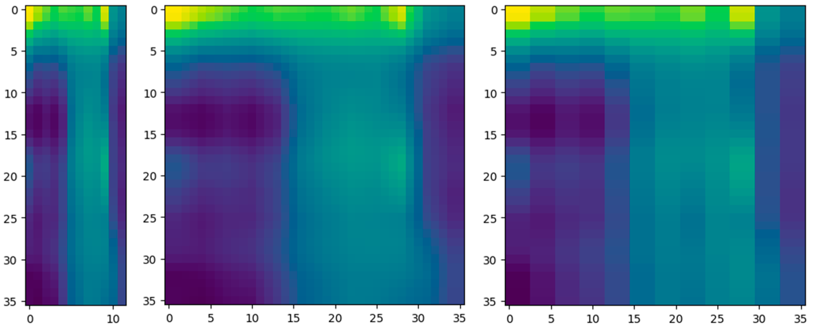
2.4. Image Representation of Multi-Spectral Time Series for Regression Task

In this paper, we introduce an additional representation of the source data. We converted the multi-spectral time series (considering the available set of bands of Sentinel-2 platforms) into a set of images wherein each image represents a given pixel over temporal and spectral dimensions. The process used to generate the images can be summarized as follows. We create an image of size m × n where m is the overall number of days or weeks starting from the reference image and n is the number of bands, which, in our case, is 12. Figure 5 shows an example of images generated from our dataset, considering both week and day resolutions.
The domain change (time series to image) opens new way to analyze data. In this case, it is possible to train models that are designed to work with images (e.g., VGG16, VGG19, MobileNet v2) by adapting network to manage the regression task (adding, at the end, dense layers with the last one linearly activated). Images can be generated starting from real time series or we can use predicted time series using the above-mentioned approaches to “cover” all the seasons. As in the case of PLS regression, several performance metrics are performed to evaluate the results.

3. Results

In this section, we present the results for the two different approaches used in this work to estimate durum wheat yield. The results of PLS regression on NDVI and NDRE functional time series are presented in the first sub-section while the second reports the image-based regression using deep learning techniques. The most relevant metrics, Mean Absolute Error (MAE), Mean Absolute Percentage Error (MAPE), Mean Squared Error (MSE), Root Mean Squared Error (RMSE), and correlation R2, are reported. Only areas with valid yields that varied from 2000 kg/ha to 9000 kg/ha, which are reasonable values, were processed. Other values could be considered as outliers due to problems related to the acquisition process (e.g., tractor’s speed). As baseline, we consider the PLS. According to several authors, when using remote sensing data, the PLS regression models can substantially improve the accuracy of yield estimation [46]. PLS aims to find a set of latent components that capture the maximum covariance between the predictor variables and the target variable. These latent components are linear combinations of the original variables. This approach can help the estimates in cases when the dependent variables are predicted by a set of regressors (e.g., NDVI time series) that have shown a strong cross-correlation [47]

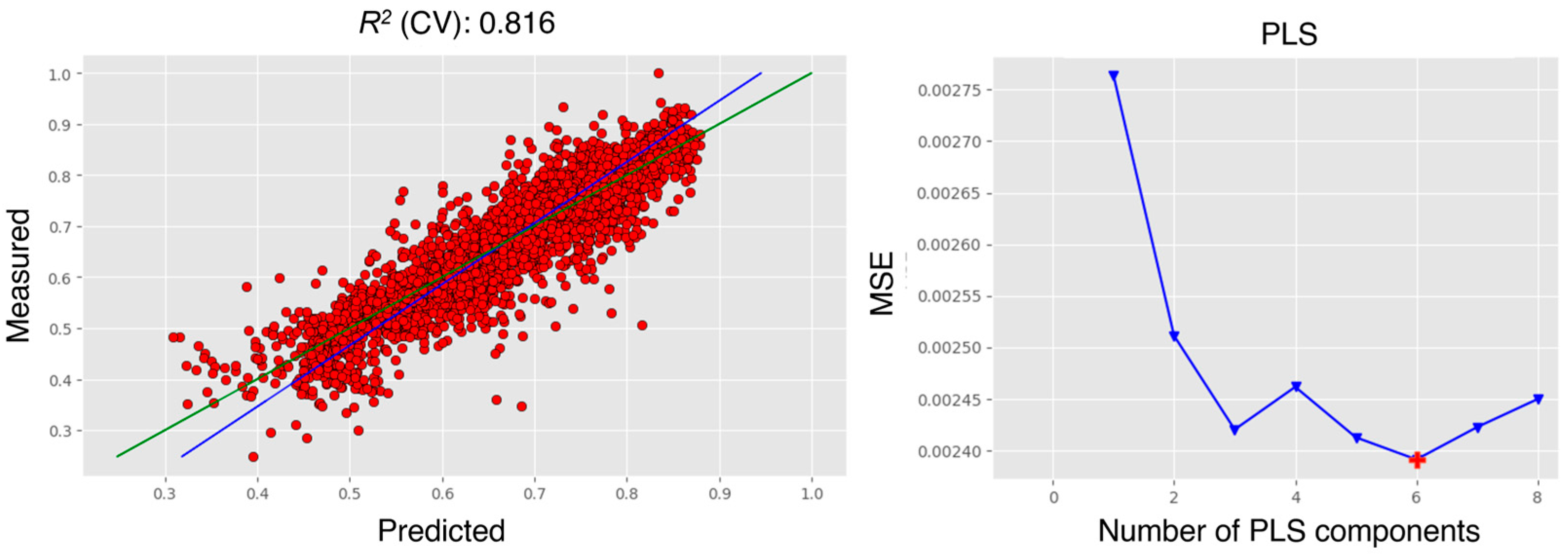
3.1. PLS Regression on Functional Time Series

In this sub-section, we summarize the results of regression on yield data, considering different scenarios. We performed the analysis starting from the functional representation of the NDVI and NDRE. This kind of approach could also be extended to other indexes. Table 1 summarizes the obtained results using 10-fold cross validation and PLS with the maximum number of components set to nine from the time series derived using the pipeline described in the previous section (i.e., Section 2). The period “week 10–36” (T1) represents the full season excluding the preliminary stages (seeding and emergence). During the season, of course, the interesting window is w10–23 (T2); in this period, correction actions (agronomic operations) could be performed. For all the cases summarized in Table 1 the correlation with the final yield varies from 0.77 to 0.82. Of course, it could be possible to use the model trained on w10–36 also during the season if we replace missing periods/values with predicted ones using the approaches described in Section 2.3. We adopted the NDVI and NDRE as reference vegetation indexes considering that they have been proven to have high correlations with the final yield. It is interesting to consider that the NDRE outperformed the NDVI, and this reflects the importance of the NDRE index to support the estimation of final yield.
Figure 6 shows the scatter plot of predicted and measured values for the NDRE and T1 temporal window and the trend of MSE according to the number of PLS components. The yield values have been scaled using a min–max approach.
An interesting perspective is the capability to train deep learning models to predict the future values of vegetation indexes such as the NDVI and NDRE that could be used also to evaluate the uniformity of ripening and maturity [11]. This plays a key role in the middle of the season, when the farmer can take decisions (e.g., foliar fertilization).

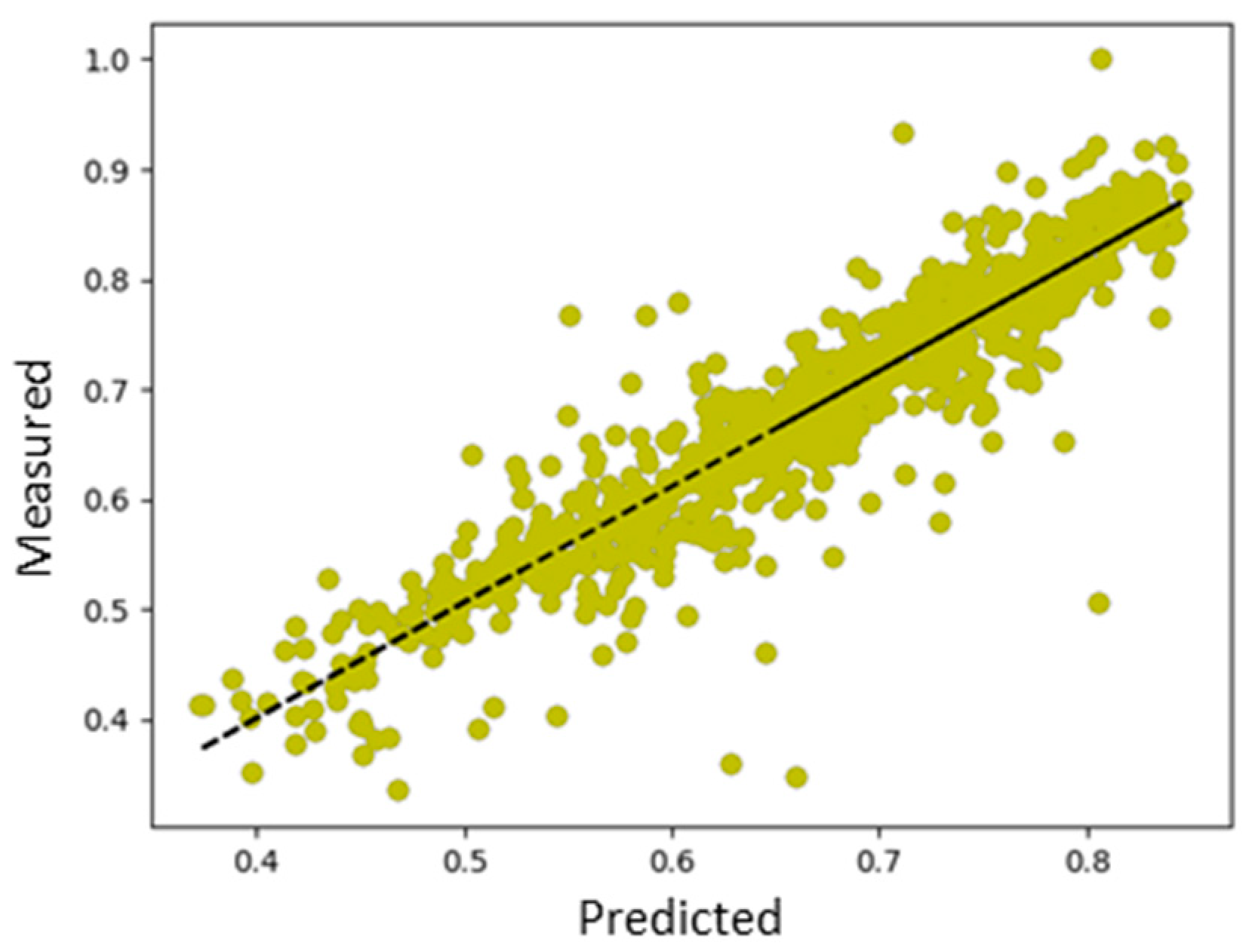
3.2. Image Based Regression Using Deep Learning

In this sub-section, we summarize the regression based on the image approach described in Section 2. This approach considers all the Sentinel-2 bands with different configurations in terms of weeks. In this case, we consider different temporal windows to understand the relationship between historical data and the final yield. The predicted values could be used to derive a potential yield map using a regression approach.
The main difference with the previous approach is that we consider all the bands over the selected time frame, trying to capture the complex interaction of time and spectral axes. VGG16, VGG19, and MobileNet v2 have been adapted to perform a regression task by adding fully connected layers. These models were trained utilizing the Gradient Descent and the Adam optimization algorithm.
The selected loss function was the MSE. We also implemented a basic convolutional network that has a 2D convolution layer followed by a 2D max pooling and three dense layers (512 + dropout 0.1, 256, and 128 activated using ReLU) followed by a last layer with linear activation for the regression.
Table 2 summarizes the results with different temporal windows, T1 and T2, as in the case of PLS. The images have been resized according to the square input size of the above-mentioned networks using nearest-neighbor and linear interpolation.
It is interesting to consider that the R2 values in both the T1 and T2 windows in the best cases are over 0.83. The linear interpolation performs better than the nearest-neighbor approach, capturing, in a more performant way, the temporal and spectral relationships behind the remotely sensed time series. Figure 7 shows the effect of interpolation, starting from the basic image that represents time (rows) and bands (columns).
Figure 8 shows the scatter plot in the best case for T1 using linear interpolation and the VGG16 model.
As in the case of PLS, it should be interesting to predict the future values of each band over time. One of the main limitations is that the models were trained using two different temporal windows. The most relevant window, of course, is the mid-season, considering that the farmer still has time to evaluate potential operations. It should be useful to estimate the values of each band over future intervals to exploit the benefits of a full-season model that has demonstrated higher performance. The developed models can be used to estimate the yield in surrounding areas where the same crop variety and similar soil conditions are available. The above-mentioned approach could also be used in cases involving multiple seasons. It is possible to have a multi-channel image as input (one channel per season), or images can be stacked on the time axis.

4. Discussion

4.1. Availability of Yield-Calibrated Data on Different Varieties

Today, there are several remotely sensed data that could be used to monitor a crop. Some platforms can deliver daily images with global coverage (e.g., Planet with PlanetScope data). The positive effect related to the availability of data could be dampened by the lack of equipment on the field that are able to acquire yield data.
In several EU countries, the use of agriculture 4.0 (AG4.0) technologies is still relatively low due to strong barriers existing on both the demand and supply sides (e.g., low awareness of potential benefits, lack of knowledge) [48,49]. In Italy, despite the public fundings dedicated to the digital transition along the agri-food supply chain, farmers are still reluctant to update their assets, and it is estimated that in 2022, only about 8% of the land for agricultural use was managed using state-of-the-art AG4.0 solutions [48,49,50]. This is still a small value, and it is strategic to collect data during the execution of agronomic operations to maximize the effect on a crop, reducing, where possible, the quantity of the product (i.e., variable rate for nutrient management).
The availability of yield data combined with remotely sensed data enables different scenarios such as the refinement of fertilization plans or the optimal designing of field sampling campaigns [51]. Yield data can also be used at different spatial scales (region, territory, etc.) to support the understanding of performance, also estimating the potential food loss. Yield mapping allows farmers to benchmark their performance against regional or industry averages. By participating in yield competitions or sharing anonymized data with fellow farmers, they can gain insights into best practices, learn from each other, and drive continuous improvement in their operations.
Calibration is another key aspect that can help the accuracy of forecasting models. Factors like crop maturity, moisture content, harvesting speed, or machine settings can affect the performance of the yield sensor, and for this reason, a calibration procedure must be performed to ensure that the gathered data reflects the real status of the field [52,53].

4.2. Factors Influencing/Impacting the Accuracy of the Regression Models

The obtained results confirm that by using remotely sensed time series based on Sentinel-2 L2A data, it is possible to estimate the crop yield with an acceptable accuracy (values greater than 0.8 for R2 suggest that the estimated yield could be used to take decisions). The obtained values in terms of the R2 MAPE and RMSE in both temporal windows suggest that predicted maps could be used to support farmers and consortia. For farmers, accurate yield predictions enable the optimization of resources such as water, fertilizers, and pesticides (where allowed). By knowing the potential yield, farmers can allocate these resources more efficiently, reducing costs and minimizing environmental impact. For consortia, yield prediction is fundamental for planning the logistics of harvesting, storage, and transportation, but also it could be used to optimize the contracts with farmers. Of course, in cases involving consortia where several farmers from different areas/districts confer their harvest, we should consider that more complex trials should be executed, considering multiple crop varieties, also with different agronomic practices (e.g., traditional, organic, zero tillage). Exogenous factors such as drought, flooding, and weeds can also impact the accuracy of the models. Their effects, in some cases, could be mitigated with well-designed and implemented agronomic practices. As already mentioned, the calibration of collected data (not only yield) plays a significant role, and preliminary checks on the quality of the data must be performed. It could be complex to fuse data from different platforms as in the case of satellites and unmanned aerial vehicles.
Another important aspect that influences the quality of regression in the co-registration of satellite data with the yield map. If we consider satellites as Sentinel-2, we have bands with different GSD values (e.g., 10, 20 m), and in such cases, the sizes of the header attached to the combine could match. The evaluation of higher-resolution imagery as in the case of PlanetScope will be investigated, but it is important to consider that the spectral resolution is limited to a few bands, mostly focused on the visible and infrared ranges [54]. Different data sources including PlanetScope and Sentinel-2 can be combined with topographic and climatic variables to properly estimate the yield [13]. Of course, it is necessary to select a proper set of vegetation indexes, but the approach presented in this paper can consider, at the same time, all the spectral bands over time. Of course, it will be necessary to compensate for the lack of spectral bands for some platforms (e.g., PlanetScope). The integration of UAV data could be an interesting point even if application to large areas could be a potential bottleneck [55].

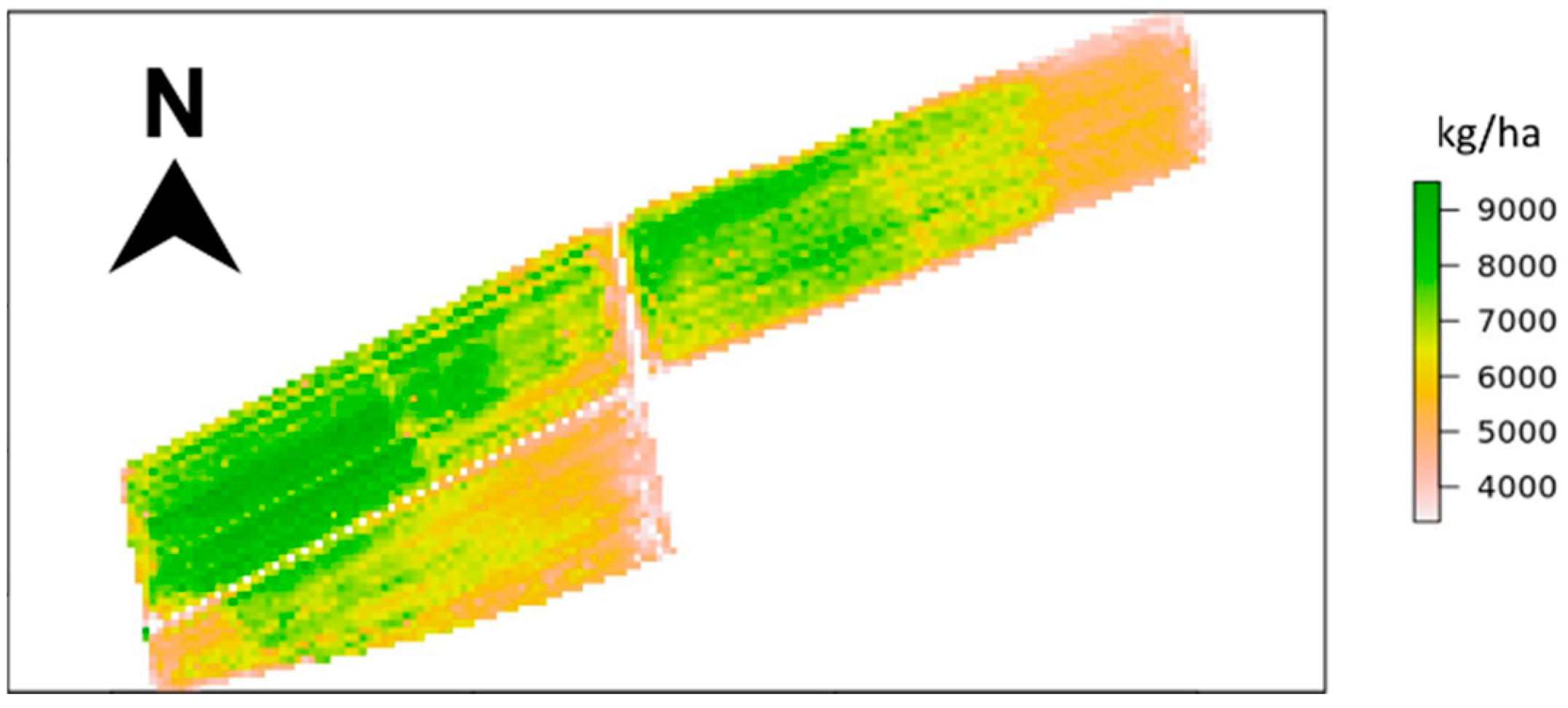
4.3. Crop Yield Distribution Map and Future Development

We estimated the yield considering different temporal windows. Of course, if we consider the overall season, we derive the best results according to the selected metrics. However, this kind of approach cannot be used during the season; it is necessary to detect problems as soon as possible to plan and execute corrective actions (agronomic operations) to mitigate the effect of the final yield. For this reason, the estimation must consider shorter temporal windows. However, deep learning could be used to predict missing values, and then the predicted curves could be used to predict the final yield using state-of-the-art approaches such as Facebook Project and NeuralProphet; the prediction of phenological curves for each spectral band could be then used to estimate the ripening period, which is really important information for different stakeholders (i.e., farmers and consortia). On the contrary, the models could be trained on shorter windows, but in this case, we are not considering the historical data as in the case of the forecast. The capability to refine models considering historical data (multiple seasons) is limited by the crop rotation, which could impose constraints regarding the temporal spacing (e.g., three-year crop rotation significantly reduces the amount of historical yield data that could be used to train models). In this context, we consider that remote and proximal sensing will play a significant role in predicting the yield and the use of digital solutions will support the transition to smart farming, also in areas where traditional approaches are dominating today [56].

5. Conclusions

In this paper, we successfully developed and tested an approach based on deep learning to perform a regression task from both remotely sensed time-series data derived from Sentinel-2 L2A and field-measured yields. Despite the CNN models showing good results (R2 values > 0.8), to further improve the model prediction accuracy and reliability, remotely sensed data must be integrated with reliable ground-based observations and other relevant field data. For instance, the accuracy of the estimates could be affected by several factors related to the data acquisition, such as the lack of alignment between the combined harvester used to monitor the yield data and the GSD of the Sentinel-2 images.
Therefore, to fully benefit from the advantages offered by these prediction models, it is of crucial importance for farmers in the supply chain to adopt precision agriculture technologies that can guarantee high levels of performance in both data acquisition and elaboration. This aspect is more crucial in the case of different field management, as in the case of the organic sector. The results of this work show that yield estimation from remotely sensed time series can provide timely, spatially explicit, and objective information on crop growth and productivity. This information can aid actors in the wheat supply chain in making informed decisions regarding crop management, resource allocation, and market strategies. From the farmers’ point of view, the novel method supports the efficient generation of a fertilization prescription map, ensuring that the fertilization plans are managed according to the crop needs, thus ensuring farm sustainability from both economic and environmental perspectives.
As future works, the evaluation and/or integration of different satellite imagery sources (e.g., PlanetScope) will be investigated, evaluating the effect of having a lower number of spectral bands. Another point of interest for future research will be the explainability of the developed model. It will be interesting to evaluate which areas in the images (temporal and spectral axes) have more importance than others [57]. The integration of multiple seasons will also be an area of investigation, considering that, in this case, the presented approach could be extended.

Author Contributions

Conceptualization, A.M., F.S. and R.Z.; methodology, A.M., L.C., F.S. and R.Z.; software, A.M. and L.C.; validation, F.M.M. and S.M.; data curation, L.C. and F.M.M.; writing—original draft preparation, S.M. and F.M.M.; writing—review and editing, A.M. and F.S.; funding acquisition, F.S. and R.Z. All authors have read and agreed to the published version of the manuscript.

Funding

This research was funded by Measure 16.1 of the 2014–2020 Marche Region RDP program through the project “BIOCEREAL 4.0”, grant agreement 29226.

Data Availability Statement

The detailed grain yield data are not available due to third-party restrictions.

Acknowledgments

The authors want to thank the partners of BIOCEREALS 4.0, APRA SpA, and Montebello Cooperativa Agrobiologica and the master’s degree students Scalella S. and Zhang Y. for their technical support. The authors also thank ENOGIS SRL for the technical support. The authors want to thank Simone Pesaresi at D3A, Università Politecnica delle Marche, Ancona, IT for his support to adapt the FPCA approach.

Conflicts of Interest

The authors declare no conflicts of interest.

References

  1. Cappelli, A.; Cini, E. Challenges and Opportunities in Wheat Flour, Pasta, Bread, and Bakery Product Production Chains: A Systematic Review of Innovations and Improvement Strategies to Increase Sustainability, Productivity, and Product Quality. Sustainability 2021, 13, 2608. [Google Scholar] [CrossRef]
  2. Altamore, L.; Ingrassia, M.; Columba, P.; Chironi, S.; Bacarella, S. Italian Consumers’ Preferences for Pasta and Consumption Trends: Tradition or Innovation? J. Int. Food Agribus. Mark. 2020, 32, 337–360. [Google Scholar] [CrossRef]
  3. Beres, B.L.; Rahmani, E.; Clarke, J.M.; Grassini, P.; Pozniak, C.J.; Geddes, C.M.; Porker, K.D.; May, W.E.; Ransom, J.K. A Systematic Review of Durum Wheat: Enhancing Production Systems by Exploring Genotype, Environment, and Management (G × E × M) Synergies. Front. Plant Sci. 2020, 11, 568657. [Google Scholar] [CrossRef] [PubMed]
  4. Guo, J.; Tanaka, T. Determinants of International Price Volatility Transmissions: The Role of Self-Sufficiency Rates in Wheat-Importing Countries. Palgrave Commun. 2019, 5, 124. [Google Scholar] [CrossRef]
  5. Cinar, G. Price Volatility Transmission among Cereal Markets. The Evidences for Turkey. New Medit. 2018, 17, 93–104. [Google Scholar] [CrossRef]
  6. Nyéki, A.; Neményi, M. Crop Yield Prediction in Precision Agriculture. Agronomy 2022, 12, 2460. [Google Scholar] [CrossRef]
  7. van der Velde, M.; Biavetti, I.; El-Aydam, M.; Niemeyer, S.; Santini, F.; van den Berg, M. Use and Relevance of European Union Crop Monitoring and Yield Forecasts. Agric. Syst. 2019, 168, 224–230. [Google Scholar] [CrossRef]
  8. Reynolds, M.P.; Braun, H.-J. Wheat Improvement; Springer Nature: Berlin/Heidelberg, Germany, 2022; ISBN 9783030906726. [Google Scholar]
  9. Wilcox, J.; Makowski, D. A Meta-Analysis of the Predicted Effects of Climate Change on Wheat Yields Using Simulation Studies. Field Crops Res. 2014, 156, 180–190. [Google Scholar] [CrossRef]
  10. Maestrini, B.; Basso, B. Predicting Spatial Patterns of Within-Field Crop Yield Variability. Field Crops Res. 2018, 219, 106–112. [Google Scholar] [CrossRef]
  11. Coviello, L.; Martini, F.M.; Cesaretti, L.; Pesaresi, S.; Solfanelli, F.; Mancini, A. Clustering of Remotely Sensed Time Series Using Functional Principal Component Analysis to Monitor Crops. In Proceedings of the 2022 IEEE Workshop on Metrology for Agriculture and Forestry, MetroAgriFor 2022–Proceedings, Perugia, Italy, 3–5 November 2022; pp. 141–145. [Google Scholar] [CrossRef]
  12. Bregaglio, S.; Ginaldi, F.; Raparelli, E.; Fila, G.; Bajocco, S. Improving Crop Yield Prediction Accuracy by Embedding Phenological Heterogeneity into Model Parameter Sets. Agric. Syst. 2023, 209, 103666. [Google Scholar] [CrossRef]
  13. Engen, M.; Sandø, E.; Sjølander, B.L.O.; Arenberg, S.; Gupta, R.; Goodwin, M. Farm-Scale Crop Yield Prediction from Multi-Temporal Data Using Deep Hybrid Neural Networks. Agronomy 2021, 11, 2576. [Google Scholar] [CrossRef]
  14. Filippi, P.; Jones, E.J.; Wimalathunge, N.S.; Somarathna, P.D.S.N.; Pozza, L.E.; Ugbaje, S.U.; Jephcott, T.G.; Paterson, S.E.; Whelan, B.M.; Bishop, T.F.A. An Approach to Forecast Grain Crop Yield Using Multi-Layered, Multi-Farm Data Sets and Machine Learning. Precis. Agric. 2019, 20, 1015–1029. [Google Scholar] [CrossRef]
  15. Segarra, J.; Araus, J.L.; Kefauver, S.C. Farming and Earth Observation: Sentinel-2 Data to Estimate within-Field Wheat Grain Yield. Int. J. Appl. Earth Obs. Geoinf. 2022, 107, 102697. [Google Scholar] [CrossRef]
  16. Saravia, D.; Valqui-Valqui, L.; Salazar, W.; Quille-Mamani, J.; Barboza, E.; Porras-Jorge, R.; Injante, P.; Arbizu, C.I. Yield Prediction of Four Bean (Phaseolus vulgaris) Cultivars Using Vegetation Indices Based on Multispectral Images from UAV in an Arid Zone of Peru. Drones 2023, 7, 325. [Google Scholar] [CrossRef]
  17. Marino, S. Understanding the Spatio-Temporal Behavior of Crop Yield, Yield Components and Weed Pressure Using Time Series Sentinel-2-Data in an Organic Farming System. Eur. J. Agron. 2023, 145, 126785. [Google Scholar] [CrossRef]
  18. Marino, S.; Alvino, A. Detection of Homogeneous Wheat Areas Using Multi-Temporal UAS Images and Ground Truth Data Analyzed by Cluster Analysis. Eur. J. Remote Sens. 2018, 51, 266–275. [Google Scholar] [CrossRef]
  19. Fraisse, C.; Ampatzidis, Y.; Guzmán, S.; Lee, W.; Martinez, C.; Shukla, S.; Singh, A.; Yu, Z. Artificial Intelligence (AI) for Crop Yield Forecasting. Edis 2022, 2022. [Google Scholar] [CrossRef]
  20. Iizumi, T.; Shin, Y.; Kim, W.; Kim, M.; Choi, J. Global Crop Yield Forecasting Using Seasonal Climate Information from a Multi-Model Ensemble. Clim. Serv. 2018, 11, 13–23. [Google Scholar] [CrossRef]
  21. Klerkx, L.; Jakku, E.; Labarthe, P. A Review of Social Science on Digital Agriculture, Smart Farming and Agriculture 4.0: New Contributions and a Future Research Agenda. NJAS-Wagening. J. Life Sci. 2019, 90–91, 100315. [Google Scholar] [CrossRef]
  22. Ghazaryan, G.; Skakun, S.; Konig, S.; Rezaei, E.E.; Siebert, S.; Dubovyk, O. Crop Yield Estimation Using Multi-Source Satellite Image Series and Deep Learning. Int. Geosci. Remote Sens. Symp. (IGARSS) 2020, 5163–5166. [Google Scholar] [CrossRef]
  23. Mahore, P.S.; Bardekar, A.A. A Review on Forecasting Agricultural Demand and Supply with Crop Price Estimation Using Machine Learning Methodologies. Int. J. Sci. Res. Comput. Sci. Eng. Inf. Technol. 2021, 3307, 570–575. [Google Scholar] [CrossRef]
  24. Bacco, M.; Barsocchi, P.; Ferro, E.; Gotta, A.; Ruggeri, M. The Digitisation of Agriculture: A Survey of Research Activities on Smart Farming. Array 2019, 3–4, 100009. [Google Scholar] [CrossRef]
  25. Reichardt, M.; Jürgens, C.; Klöble, U.; Hüter, J.; Moser, K. Dissemination of Precision Farming in Germany: Acceptance, Adoption, Obstacles, Knowledge Transfer and Training Activities. Precis. Agric. 2009, 10, 525–545. [Google Scholar] [CrossRef]
  26. Xu, Z.; Cannon, S.B.; Beavis, W.D. Applying Spatial Statistical Analysis to Ordinal Data for Soybean Iron Deficiency Chlorosis. Agronomy 2022, 12, 2095. [Google Scholar] [CrossRef]
  27. Niedbała, G.; Wróbel, B.; Piekutowska, M.; Zielewicz, W.; Paszkiewicz-Jasińska, A.; Wojciechowski, T.; Niazian, M. Application of Artificial Neural Networks Sensitivity Analysis for the Pre-Identification of Highly Significant Factors Influencing the Yield and Digestibility of Grassland Sward in the Climatic Conditions of Central Poland. Agronomy 2022, 12, 1133. [Google Scholar] [CrossRef]
  28. Reinhardt, T. The Farm to Fork Strategy and the Digital Transformation of the Agrifood Sector—An Assessment from the Perspective of Innovation Systems. Appl. Econ. Perspect. Policy 2022, 45, 819–838. [Google Scholar] [CrossRef]
  29. Basso, B.; Antle, J. Digital Agriculture to Design Sustainable Agricultural Systems. Nat. Sustain. 2020, 3, 254–256. [Google Scholar] [CrossRef]
  30. Wesseler, J. The EU’s Farm-to-Fork Strategy: An Assessment from the Perspective of Agricultural Economics. Appl. Econ. Perspect. Policy 2022, 44, 1826–1843. [Google Scholar] [CrossRef]
  31. Rembold, F.; Meroni, M.; Urbano, F.; Royer, A.; Atzberger, C.; Lemoine, G.; Eerens, H.; Haesen, D. Remote Sensing Time Series Analysis for Crop Monitoring with the SPIRITS Software: New Functionalities and Use Examples. Front. Environ. Sci. 2015, 3, 46. [Google Scholar] [CrossRef]
  32. Sedighkia, M.; Fathi, Z.; Abdoli, A. Minimizing Environmental Impacts of Apple Production by Linking Yield Prediction Model and Water–Energy Resources’ Optimization. Model. Earth Syst. Environ. 2023, 9, 1233–1249. [Google Scholar] [CrossRef]
  33. Panek, E.; Gozdowski, D. Analysis of Relationship between Cereal Yield and NDVI for Selected Regions of Central Europe Based on MODIS Satellite Data. Remote Sens. Appl. 2020, 17, 100286. [Google Scholar] [CrossRef]
  34. Romano, E.; Bergonzoli, S.; Pecorella, I.; Bisaglia, C.; De Vita, P. Methodology for the Definition of Durum Wheat Yield Homogeneous Zones by Using Satellite Spectral Indices. Remote Sens. 2021, 13, 2036. [Google Scholar] [CrossRef]
  35. Dey, S.; Bhogapurapu, N.; Homayouni, S.; Bhattacharya, A.; McNairn, H. Unsupervised Classification of Crop Growth Stages with Scattering Parameters from Dual-Pol Sentinel-1 SAR Data. Remote Sens. 2021, 13, 4412. [Google Scholar] [CrossRef]
  36. Bajocco, S.; Vanino, S.; Bascietto, M.; Napoli, R. Exploring the Drivers of Sentinel-2-Derived Crop Phenology: The Joint Role of Climate, Soil, and Land Use. Land 2021, 10, 656. [Google Scholar] [CrossRef]
  37. Yli-Heikkila, M.; Wittke, S.; Luotamo, M.; Puttonen, E.; Sulkava, M.; Pellikka, P.; Heiskanen, J.; Klami, A. Scalable Crop Yield Prediction with Sentinel-2 Time Series and Temporal Convolutional Network. Remote Sens. 2022, 14, 4193. [Google Scholar] [CrossRef]
  38. van Klompenburg, T.; Kassahun, A.; Catal, C. Crop Yield Prediction Using Machine Learning: A Systematic Literature Review. Comput. Electron. Agric. 2020, 177, 105709. [Google Scholar] [CrossRef]
  39. Muruganantham, P.; Wibowo, S.; Grandhi, S.; Samrat, N.H.; Islam, N. A Systematic Literature Review on Crop Yield Prediction with Deep Learning and Remote Sensing. Remote Sens. 2022, 14, 1990. [Google Scholar] [CrossRef]
  40. Sun, J.; Di, L.; Sun, Z.; Shen, Y.; Lai, Z. County-Level Soybean Yield Prediction Using Deep CNN-LSTM Model. Sensors 2019, 19, 4363. [Google Scholar] [CrossRef]
  41. Kiran Kumar, V.; Ramesh, K.V.; Rakesh, V. Optimizing LSTM and Bi-LSTM Models for Crop Yield Prediction and Comparison of Their Performance with Traditional Machine Learning Techniques. Appl. Intell. 2023, 53, 28291–28309. [Google Scholar] [CrossRef]
  42. Ullah, S.; Finch, C.F. Applications of Functional Data Analysis: A Systematic Review. BMC Med. Res. Methodol. 2013, 13, 43. [Google Scholar] [CrossRef]
  43. Pesaresi, S.; Mancini, A.; Quattrini, G.; Casavecchia, S. Mapping Mediterranean Forest Plant Associations and Habitats with Functional Principal Component Analysis Using Landsat 8 NDVI Time Series. Remote Sens. 2020, 12, 1132. [Google Scholar] [CrossRef]
  44. Han, K.; Hadjipantelis, P.Z.; Wang, J.L.; Kramer, M.S.; Yang, S.; Martin, R.M.; Müller, H.G. Functional Principal Component Analysis for Identifying Multivariate Patterns and Archetypes of Growth, and Their Association with Long-Term Cognitive Development. PLoS ONE 2018, 13, e0207073. [Google Scholar] [CrossRef] [PubMed]
  45. Karuppusami, R.; Antonisamy, B.; Premkumar, P.S. Functional Principal Component Analysis for Identifying the Child Growth Pattern Using Longitudinal Birth Cohort Data. BMC Med. Res. Methodol. 2022, 22, 76. [Google Scholar] [CrossRef] [PubMed]
  46. Zhang, P.P.; Zhou, X.X.; Wang, Z.X.; Mao, W.; Li, W.X.; Yun, F.; Guo, W.S.; Tan, C.W. Using HJ-CCD Image and PLS Algorithm to Estimate the Yield of Field-Grown Winter Wheat. Sci. Rep. 2020, 10, 5173. [Google Scholar] [CrossRef] [PubMed]
  47. Lopez-Fornieles, E.; Brunel, G.; Rancon, F.; Gaci, B.; Metz, M.; Devaux, N.; Taylor, J.; Tisseyre, B.; Roger, J.M. Potential of Multiway PLS (N-PLS) Regression Method to Analyse Time-Series of Multispectral Images: A Case Study in Agriculture. Remote Sens. 2022, 14, 216. [Google Scholar] [CrossRef]
  48. Scuderi, A.; La Via, G.; Timpanaro, G.; Sturiale, L. The Digital Applications of “Agriculture 4.0”: Strategic Opportunity for the Development of the Italian Citrus Chain. Agriculture 2022, 12, 400. [Google Scholar] [CrossRef]
  49. Long, T.B.; Blok, V.; Coninx, I. Barriers to the Adoption and Diffusion of Technological Innovations for Climate-Smart Agriculture in Europe: Evidence from the Netherlands, France, Switzerland and Italy. J. Clean. Prod. 2016, 112, 9–21. [Google Scholar] [CrossRef]
  50. Osservatorio Smart AgriFood L’agricoltura 4.0 Italiana Sfonda Il Muro Dei 2 Miliardi Di Euro Nel 2022, +31%. Available online: https://www.osservatori.net/it/ricerche/comunicati-stampa/agricoltura-4-0-mercato (accessed on 10 November 2023).
  51. Ali, A.M.; Abouelghar, M.; Belal, A.A.; Saleh, N.; Yones, M.; Selim, A.I.; Amin, M.E.S.; Elwesemy, A.; Kucher, D.E.; Maginan, S.; et al. Crop Yield Prediction Using Multi Sensors Remote Sensing (Review Article). Egypt. J. Remote Sens. Space Sci. 2022, 25, 711–716. [Google Scholar] [CrossRef]
  52. Sun, Y.; Liu, R.; Zhang, M.; Li, M.; Zhang, Z.; Li, H. Design of Feed Rate Monitoring System and Estimation Method for Yield Distribution Information on Combine Harvester. Comput. Electron. Agric. 2022, 201, 107322. [Google Scholar] [CrossRef]
  53. Ping, J.L.; Dobermann, A. Processing of Yield Map Data. Precis. Agric. 2005, 6, 193–212. [Google Scholar] [CrossRef]
  54. Farmonov, N.; Amankulova, K.; Szatmári, J.; Urinov, J.; Narmanov, Z.; Nosirov, J.; Mucsi, L. Combining PlanetScope and Sentinel-2 Images with Environmental Data for Improved Wheat Yield Estimation. Int. J. Digit. Earth 2023, 16, 847–867. [Google Scholar] [CrossRef]
  55. Sagan, V.; Maimaitijiang, M.; Bhadra, S.; Maimaitiyiming, M.; Brown, D.R.; Sidike, P.; Fritschi, F.B. Field-Scale Crop Yield Prediction Using Multi-Temporal WorldView-3 and PlanetScope Satellite Data and Deep Learning. ISPRS J. Photogramm. Remote Sens. 2021, 174, 265–281. [Google Scholar] [CrossRef]
  56. Darra, N.; Anastasiou, E.; Kriezi, O.; Lazarou, E.; Kalivas, D.; Fountas, S. Can Yield Prediction Be Fully Digitilized? A Systematic Review. Agronomy 2023, 13, 2441. [Google Scholar] [CrossRef]
  57. Letzgus, S.; Wagner, P.; Lederer, J.; Samek, W.; Muller, K.R.; Montavon, G. Toward Explainable Artificial Intelligence for Regression Models: A Methodological Perspective. IEEE Signal Process Mag. 2022, 39, 40–58. [Google Scholar] [CrossRef]
Figure 1. Processing pipeline for remotely sensed time series to estimate the yield using satellite data and historical yield data.
Agronomy 14 00109 g001
Figure 2. Yield map over the study area (the data are estimations of real yield; the combine’s speed could have impacted both the overall accuracy as well the calibration of the sensors that were reserved).
Agronomy 14 00109 g002
Figure 3. Example of spline representation of the NDVI index over the fields. x-axis represents the week number from first image. On the y-axis, we report the value of the NDVI index.
Agronomy 14 00109 g003
Figure 4. Different configurations of reconstructed time series using the FCPA. Top left: original set of curves. Top right: reconstructed using 1 component. Bottom left: reconstructed using 2 components. Bottom right: reconstructed using 3 components. The x-axis represents the week number from first image. On the y-axis, we report the value of the NDVI index.
Agronomy 14 00109 g004
Figure 5. Left: example of image generated from a pixel using the week as unit. Right: example of image generated from a pixel using the day as unit and considering a limited number of days.
Agronomy 14 00109 g005
Figure 6. Left: scatter plot of predicted and measured scaled yields. Blue line is the best fit line while the green one represents the 1:1 line. Yield values are normalized in the interval 0–95th percentile. Right: trend of MSE according to the number of PLS components (in that case, six components represent the optimal choice).
Agronomy 14 00109 g006
Figure 7. Left: example of image generated from a pixel using the week as unit. Middle: resampling to square size using linear interpolation. Right: resampling to square size using nearest-neighbor interpolation.
Agronomy 14 00109 g007
Figure 8. Scatter plot for VGG16 model with linear interpolation over T1 temporal window. The dashed line represents the best fit line.
Agronomy 14 00109 g008
Table 1. Results from PLS using the time series derived from remotely sensed Sentinel-2 L2A data. A value in bold represents the best result for the considered metrics.
ModelTemporal WindowMAEMAPEMSERMSER2
NDVIT10.0380.0610.0030.0480.799
NDRET10.0360.0580.0020.0460.816
NDVIT20.0420.0670.0030.0520.770
NDRET20.0410.0660.0030.0490.786
Table 2. Regression on the yield with different temporal windows and models using the image-based approach. Suffix L stands for linear interpolation while N stands for Nearest Neighbor. A value in bold represents the best result for the considered metrics.
ModelTemporal WindowMAEMAPEMSERMSER2
VGG-16LT10.0330.0510.0020.0470.843
VGG-16NT10.0460.0760.0040.0590.720
VGG-19LT10.0380.0590.0030.0510.812
VGG-19NT10.0360.0560.0020.0480.822
MNetv2LT10.0440.0700.0030.0560.758
MNetv2NT10.0380.0580.0030.0550.783
CustomT10.0400.0580.0030.0500.822
VGG-16LT20.0420.0650.0030.0530.783
VGG-16NT20.0430.0710.0030.0570.743
VGG-19LT20.0340.0550.0020.0480.821
VGG-19NT20.0400.0620.0030.0520.790
MNetv2LT20.0330.0520.0020.0450.838
MNetv2NT20.0400.0600.0020.0500.805
CustomT20.0460.0700.0030.0560.774
Disclaimer/Publisher’s Note: The statements, opinions and data contained in all publications are solely those of the individual author(s) and contributor(s) and not of MDPI and/or the editor(s). MDPI and/or the editor(s) disclaim responsibility for any injury to people or property resulting from any ideas, methods, instructions or products referred to in the content.

