
Semantic Segmentation of Portuguese Agri-Forestry Using High-Resolution Orthophotos

MARETEC—Marine, Environment and Technology Centre, LARSyS, Instituto Superior Técnico, Universidade de Lisboa, Av. Rovisco Pais, 1, 1049-001 Lisbon, Portugal
*
Author to whom correspondence should be addressed.
Agronomy 2023, 13(11), 2741; https://doi.org/10.3390/agronomy13112741
Submission received: 14 September 2023
/
Revised: 20 October 2023
/
Accepted: 27 October 2023
/
Published: 30 October 2023
(This article belongs to the Special Issue Computer Vision and Deep Learning Technology in Agriculture)
Abstract
:The Montado ecosystem is an important agri-forestry system in Portugal, occupying about 8% of the total area of the country. However, this biodiverse ecosystem is threatened due to factors such as shrub encroachment. In this context, the development of tools for characterizing and monitoring Montado areas is crucial for their conservation. In this study, we developed a deep convolutional neural network algorithm based on the U-net architecture to identify regions with trees, shrubs, grass, bare soil, or other areas in Montado areas using high-resolution RGB and near-infrared orthophotos (with a spatial resolution of 25 cm) from seven experimental sites in the Alentejo region of Portugal (six used for training/validation and one for testing). To optimize the model’s performance, we performed hyperparameter tuning, which included adjusting the number of filters, dropout rate, and batch size. The best model achieved an overall classification performance of 0.88 and a mean intersection of the union of 0.81 on the test set, indicating high accuracy and reliability of the model in identifying and delineating land cover classes in the Montado ecosystem. The developed model is a powerful tool for identifying the status of the Montado ecosystem regarding shrub encroachment and facilitating better future management.
1. Introduction
The Montado/Dehesa ecosystem is an agro-silvopastoral system found in the Mediterranean region of Portugal and Spain, characterized by the presence of cork oak (Quercus suber) and/or hoalm oak (Quercus ilex) forests [1,2]. The Portuguese Montado occupies about 800,000 hectares, which is about 8% of the total area of Portugal [1]. The Montado ecosystem provides a range of important ecosystem services, such as carbon sequestration, water regulation, and habitat for a variety of plant and animal species [3,4,5,6]. However, the ecosystem is facing significant challenges, including shrub encroachment [7,8,9], which is causing the conversion of the underlying grassland and agricultural land into dense shrubland. This can negatively impact the productivity of the system and the provisioning of ecosystem services, as well as threaten the traditional land management practices and the cultural heritage of the region [5,10,11].
Remote sensing techniques have been extensively used to understand and monitor the Montado ecosystem [2,12,13]. Remotely sensed data can provide detailed information on land use patterns, including the distribution of different land cover types [14,15,16]. The majority of this work has been conducted using satellite data, specifically Sentinel-2 and Landsat 7–8 data [14,17]. However, due to the spatial heterogeneity of the Montado ecosystem, the spatial resolution of these data sources, which is typically 10 m, is often insufficient for detailed characterization of the land system, particularly for identifying trees and shrubs [18,19]. To overcome this limitation, high-resolution satellite imagery such as Pleiades or GEOSat, which have sub-metric spatial resolution, can be used as a viable alternative [19]. Additionally, orthophoto maps obtained from aerial images also provide higher spatial resolution [20], which is necessary for accurate identification of land cover types in the Montado ecosystem. These higher-resolution data sources can enable more precise mapping of land cover types and a better understanding of the spatial distribution and status of the Montado ecosystem, which is crucial for effective management and conservation efforts [2,21].
Recent advancements in machine learning and deep learning have provided new opportunities for the automated analysis of remote sensing data [22,23,24] and have opened new possibilities for characterizing land use systems [25,26,27]. Furthermore, deep learning approaches have reached higher performance than more traditional machine learning approaches and other methods, namely due to their ability to learn complex and nonlinear patterns in the spatial and temporal dimensions without requiring transformation of the inputs [22,28]. One of the key applications of deep learning in remote sensing is in the field of image semantic segmentation [29,30,31], which aims to divide an image into multiple segments or regions, each corresponding to a different land cover type. One of the most widely used semantic segmentation models is called U-Net [32,33], which is a convolutional neural network designed specifically for image segmentation tasks. A U-Net is trained on a set of labeled images and can then be used to classify each pixel in an image into the appropriate land cover class, making the segmentation process automatic and efficient [30,34]. The U-Net architecture consists of two main parts: the contracting path and the expansive path. The contracting path is composed of convolutional and max pooling layers that decrease the spatial resolution of the input image while simultaneously extracting high-level features. The expansive path is composed of up-sampling and deconvolutional layers that increase the spatial resolution and reconstruct the segmented image [32,33].
In this paper, we use high-resolution RGB and near-infrared orthophoto maps (25 cm spatial resolution) and deep learning techniques (U-Net) to analyze the Montado ecosystem and investigate the potential of these methods for characterizing agro-forestry systems, namely produce a model for semantic segmentation of orthophoto maps into five land cover classes (”Tree”, “Shrub”, “Grass”, “Bare”, and “Other”). To achieve this goal, we performed a hyper-parameterization optimization (number of filters, dropout rate, and batch size) of the U-Net model to improve its ability to accurately characterize the Montado ecosystem.
2. Materials and Methods
2.1. Study Area
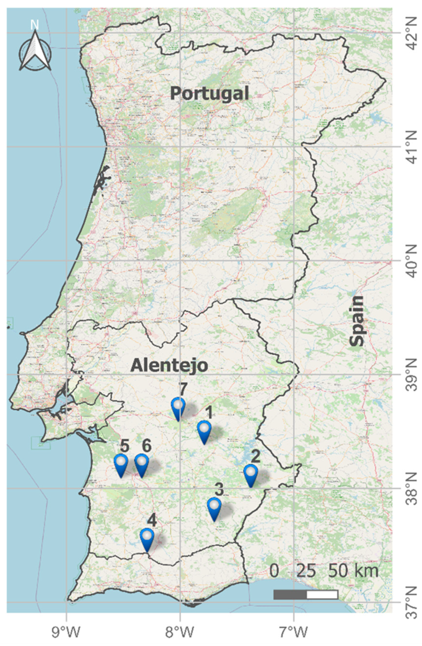
The study area selected for the experiment was the Alentejo region of Portugal, which is dominated by the Montado ecosystem. Seven experimental sites were randomly chosen within the study area, as illustrated in Figure 1. Experimental site 1 is in Évora municipality (38°34′31″ N, 7°47′18″ W). Experimental site 2 is in Moura municipality (38°11′27″ N, 7°22′46″ W). Experimental site 3 is in Serpa municipality (37°53′58″ N, 7°42′2″ W). Experimental site 4 is in Odemira municipality (37°37′48″ N, 8°17′29″ W). Experimental sites 5 and 6 are in Alcácer do Sal municipality (38°16′57″ N, 8°31′17″ W, and 38°16′59″ N, 8°20′17″ W, respectively). Experimental site 7 is in Montemor-o-Novo municipality (38°46′43″ N, 8°1′4″ W).
All experimental sites exhibit heterogeneous vegetation, encompassing trees, shrubs, grassland, bare soil, and other vegetation types. Each experimental site has an area of 1 km2, resulting in a total study area of 7 km2, which was used to train, test, and validate the models.
2.2. Used Data and Pre-Processing
The orthophotos utilized in this study were produced by the General Directorate for Territorial Development (DGT) and provided by the Portuguese Institute for Agricultural and Fisheries Financing (IFAP). The image acquisition was carried out using cameras on an airplane, specifically a high-resolution imaging system deployed by the Directorate-General for Territorial Planning (DGT) for capturing orthophoto maps in Portugal. We used orthophotos for the year 2018, which have the highest spatial resolution of 25 cm per pixel (orthophotos for the previous years—2015, 2012, and 2010—have a lower spatial resolution of 50 cm per pixel). The orthophotos used in this study consist of four bands: red (R), green (G), blue (B), and near-infrared (NIR). RGB bands provide color information that is essential for capturing the visual appearance of objects and landscapes. The NIR band provides valuable information about reflectance properties beyond the visible spectrum (e.g., NIR is more sensitive to the chlorophyll content in plants). When combined, RGB and NIR bands enable more comprehensive and accurate semantic segmentation, as they provide complementary data that enhances the ability to differentiate and categorize different land cover classes.
The aerial flights used to generate the orthophotos were conducted between June and October 2018. Orthophotos for experimental sites 1 and 7 were obtained in August, for sites 2 and 3 in September, and for sites 4, 5, and 6 in June. This collection period coincides with Portugal’s summer season, which experiences lower cloud cover and drier vegetation. This may affect the proportion between pasture and bare soil areas.
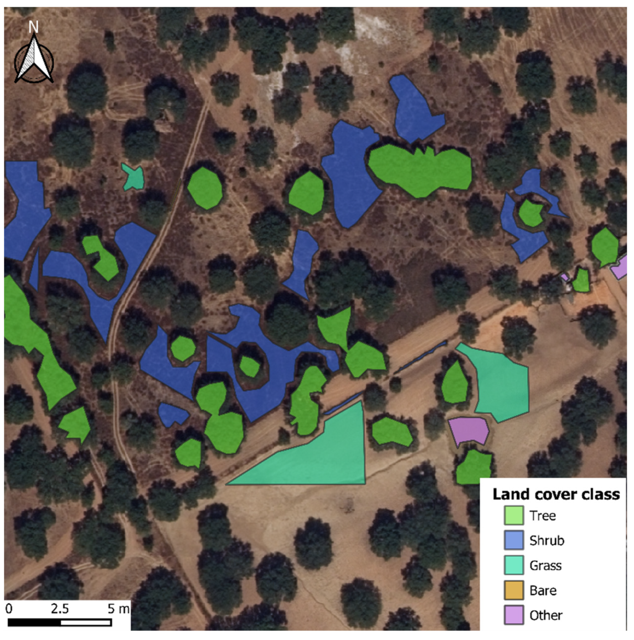
The delineation of land cover classes in the orthophotos was carried out manually by the authors. The QGIS 3.24.1 software was used to create polygons for five land cover classes: trees, shrubs, grassland, bare soil, and other areas. Approximately 100 polygons were drawn for each of the seven experimental sites. The drawn polygons at all experimental sites were sparsely distributed across the entire area. This manual delineation ensured the accuracy and reliability of the ground truth data used to train and evaluate the CNN models. Further, each experimental plot was divided into 256 px × 256 px (64 m × 64 m) individual plots.
2.3. Semantic Segmentation Model
We employed two deep learning model architectures in this work, the U-Net and the Fully Convolutional Network (FCN) model, to map land cover classes in high-resolution orthophotos. U-Net is a CNN-based algorithm that learns to recognize classes through supervised classification by fixing the weights of convolutional filters in an iterative process. The U-Net architecture comprises an encoder followed by a decoder. The encoder initially passes the input through several hidden layers, reducing the spatial resolution through the effect of down-sampling filters while simultaneously increasing the “spectral” resolution. The decoder then passes the image through additional hidden layers that reverse the process of the encoder. Therefore, in each layer, the input image loses spectral resolution while gaining spatial resolution to produce the final segmented image. For a more detailed description of the U-Net architecture, see [33]. FCN leverages a series of convolutional and pooling layers for feature extraction and then employs transposed convolutions (also known as deconvolutions) to upsample the feature maps back to the original image resolution. This enables FCNs to capture and preserve spatial information, making them well-suited for tasks like object detection, image segmentation, and even real-time applications. For a more detailed description of the FCN architecture, see [35].
In order to minimize overfitting with both models, the dropout regularization technique was used. It works by randomly (with a different choice at each training step) setting a proportion of the inputs to a layer to zero during training, forcing the network to learn more robust features [33].
The performance of both models is also influenced by the batch size, i.e., the number of training examples used in each iteration of the model training process. During training, the data are divided into batches, and the model’s parameters are updated based on the loss calculated for each batch.
In this work, as not all pixels within each plot (256 × 256 px) in the training data were classified into one of the five land cover classes, an updated version of the categorical cross-entropy loss function was used. This function assigned a null weight to unknown pixels and a weight of 1 to all classified pixels. As a result, when the model was applied to an orthophoto, all pixels in the final segmented image were assigned to one of the five land use classes; even the pixels without ground truth classification were classified. In total, 5681 images of 256 × 256 px were used in this work.
2.4. Training, Validation, and Test Approach
The individual orthophotos were split into three sets: training, validation, and test sets. The training set was used to tune the weights of the U-Net for each choice of the hyperparameters. The validation set was used to choose the hyperparameters that maximize performance. The test set was never used to train the U-Net or choose the hyperparameters, but only to assess the performance of the model in an independent set.
To achieve optimal performance, we conducted hyperparameter tuning for both model architectures, considering the number of filters (8 or 16), the dropout rate (0.05 or 0.10), and the batch size (16 or 32).
In terms of data partition, we implemented a more rigorous method than a simple random partition between training, validation, and test sets. Specifically, we designated an entire experimental site (site 7) as the test set, meaning that it was excluded from the training and hyperparameter selection phases (in total, 560 images). Meanwhile, the remaining 6 experimental sites (5121 images) were randomly divided between the training (80%) and validation (20%) sets. The training set was utilized to adjust the U-Net model’s weights; the validation set was solely used for selecting the optimal hyperparameters; and the test set was employed to evaluate the models’ performance. In this way, we tested how the model generalizes to new situations, as the error is measured in a region that is not represented in training and validation.
The packages used were Numpy 1.18.5 (https://github.com/numpy/numpy, accessed on 10 September 2023) to handle all the data processing, scikit-learn 1.0.24 for data partition, and TensorFlow 2.7 (https://github.com/tensorflow/tensorflow, accessed on 10 September 2023) to construct the CNN model architecture. A PC with 2.5 Ghz and 16 GB of RAM with CUDA was used to train and evaluate all the models.
2.5. Accuracy Assessment
In this study, we employed four performance metrics to evaluate the accuracy of our models: overall accuracy, F1 score, Cohen’s Kappa, and mean intersection of the union. Overall accuracy was computed by dividing the sum of true positives and true negatives by the total number of samples. F1-score balances precision (true positive predictions) and recall (correctly identified positive instances) using the harmonic mean. Cohen’s kappa is a statistic measuring the agreement between raters or classifiers. It considers both observed and expected agreement and provides a score from −1 (no agreement) to 1 (perfect agreement), with 0 indicating agreement by chance. The mean intersection over union (mIoU) was calculated as the ratio of the intersection of the predicted and ground truths to their union. The metrics used were therefore
where TPi denotes the number of true positive cases, FPi the number of false positive cases, TNi the number of true negative cases, FNi the number of false negative cases, N is the number of classes (here equal to 5), and i denotes each of the individual classes. With the exception of the first one, all metrics are averages over the metric values for each class.
3. Results
3.1. Analysis of the Dataset
Table 1 provides a comprehensive overview of the land cover classes identified in the study area, giving us insights into the distribution of each class. The classification results show that the “Tree” class has the highest number of polygons, indicating the presence of numerous trees in the study area. However, when looking at the number of pixels, the “Tree” class only accounts for a small percentage of the total number of pixels. This is mainly due to the nature of the Montado ecosystem in Alentejo, which is characterized by sparse tree cover. The “Shrub” class, on the other hand, has the highest number of pixels, which indicates that shrubs are the dominant vegetation type in the study area. Furthermore, the “Grass” class has a higher number of pixels than the “Tree” class, despite having a lower number of polygons. In contrast, both the “Bare” and “Other” classes have the lowest number of polygons and pixels, indicating the presence of non-vegetated areas or areas that cannot be classified into any of the five land cover classes.
Figure 2 provides an example of a plot with the polygons manually defined for the identified land covers. It is noticeable that the “Tree” class is sparser than the other land cover classes, which is consistent with the Montado ecosystem. It is worth noting that the authors did not classify all the areas in the figure. This is because there are areas without polygons identified due to two main reasons. Firstly, it can be difficult for the human eye to distinguish between some trees and shrubs, making it challenging to classify all pixels. Secondly, even if we ignore the first reason, it would not be feasible to classify the entire experimental site area. The different colors representing each class allow for a clear visualization of the distribution and relative abundance of each land cover. Overall, this figure serves as a useful tool for understanding the distribution and composition of the different land covers within the studied area.
3.2. Performance of Orthophoto Map Segmentation
The U-net outperformed the FCN for all combinations of hyperparameters, such as the number of filters, dropout rate, and batch size. In Table 2, we can observe the performance metrics for the U-net model, and in Table 3, we see results for the FCN. Given the results obtained, from hereon we only depict and interpret results for the U-net model. The lower performance of the FCN model could be attributed to its inherent design differences, such as not fully capturing the fine-grained features and spatial context essential for precise semantic segmentation, which the U-Net architecture excels at. Additionally, the U-Net model’s skip connections and expansive pathways facilitate better feature extraction and integration, making it more suitable for our specific remote sensing application.
It is evident that all the models had high performance, with an overall accuracy higher than 80%, indicating the effectiveness of the U-net model in accurately classifying land cover classes. Furthermore, the F1, Kappa, and mean IoU metrics also confirmed the high performance of the models. However, it is important to note that there are no significant differences between most of the models. Despite this, model 2, which has a configuration of 8 filters, a dropout rate of 0.05, and a batch size of 32, stands out with slightly better performance for all the metrics, except mean IoU. Therefore, this model was considered the optimum hyperparameter combination and used in the segmentation of the orthophotos.
Analyzing the performance per hyperparameter individually, models with 8 filters tend to perform better compared to models with 16 filters. For example, comparing model 1 with model 3, it can be observed that the model with eight filters performs better. Similarly, a lower dropout rate of 0.05 was found to be associated with higher performance compared to a dropout rate of 0.10. This is evident from the comparison between models 2 and 6. Although the model with the best hyperparameters had a batch size of 32, it is noteworthy that a batch size of 16 tends in general to have higher performance than a batch size of 32.
Table 4 shows that the IoU results for the “Tree”, “Shrub”, and “Other” classes were quite similar across models and hyperparameters, with values ranging from 0.70 to 0.98. This suggests that the predicted segmentation masks for these classes had a high degree of overlap with the ground truth data. However, for the “Grass” and “Bare” classes, there were significant differences in the IoU values across models and hyperparameters. Most of the models showed an IoU below 0.7 for these classes, indicating poorer performance in correctly identifying these land cover categories. Only models 2 and 5 demonstrated good performance for the “Grass” and “Bare” classes. For instance, while model 1 achieved the highest IoU score (0.98) for the “Other” class, it showed poor performance (0.39) for the “Bare” class. These findings highlight the importance of considering the IoU metric per land cover class along with the mean IoU when evaluating the segmentation models.
Table 5 presents the confusion matrix of the U-Net model with the best hyperparameters applied to the test set location. As verified previously, the model demonstrates a notably high accuracy rate in all classes. However, it exhibits, to some extent, a misclassification between the “Trees” and “Shrub” classes.
3.3. Application of the Model
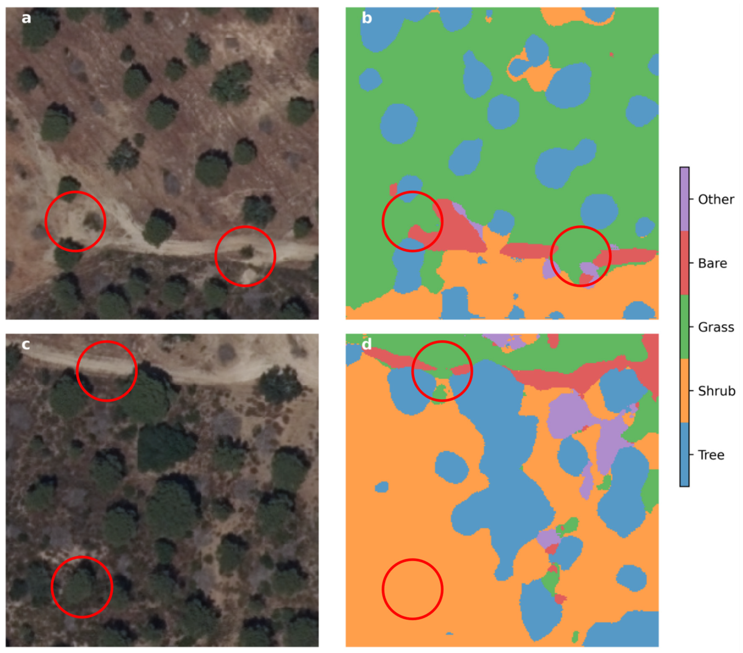
Figure 3 presents the results of applying the best-performing model, model 2, to two different locations in the test set (experimental site 7) that were not part of the training data. This example demonstrates the potential of the model, as expected considering the results presented in Table 2 and Table 3, as it was able to accurately identify the land cover classes in both locations. The model performed particularly well in identifying the “Tree” class, including small trees, and the “Shrub” class. However, in small regions, the model incorrectly classified path pixels that belong clearly to the “Bare” class as “Grass” class and also missed some trees (namely in Figure 3c,d). This limitation could be attributed to the data used in this study, as the orthophotos were primarily captured during the summer when vegetation is dry and can be misinterpreted as bare soil. Overall, these results show the promise of using deep learning models for land cover classification while also highlighting the importance of carefully considering the timing and quality of the data used.
4. Discussion
One of the main advantages of using deep learning for land use system characterization is its ability to automatically learn and extract features from large and complex datasets [23]. This is particularly useful in the case of the Montado ecosystem, where the presence of shrubs can be difficult to detect due to the presence of other land cover types, such as trees and grassland [29]. Deep learning models, such as convolutional neural networks (CNNs), have been shown to be highly effective in image classification tasks [30,31]. In this study, we showed that deep learning models (U-Net and FCN) are a feasible solution for analyzing land cover in Montado ecosystems, especially for identifying landscape features using high-resolution orthophoto maps, with U-Net outperforming the FCN in the task presented in this paper. The fine-tuning of hyperparameters enabled us to achieve the structure that performed the best in the task of orthophoto map segmentation into the five predefined land cover classes. The hyperparameters that yielded the highest performance produced an overall accuracy of about 0.88 and a mean IoU of 0.81.
The findings of this study are consistent with previous research in remote sensing image semantic segmentation. In a review of over 170 papers that performed this task, Ma et al. [36] reported an overall accuracy of approximately 0.80. It should be noted that overall accuracy varies to some degree based on the remote sensing data source used. Papers that used data from unmanned aerial vehicles (UAVs) tended to have higher overall accuracy compared to those using satellite data, indicating that proximity of the sensor can influence results. For example, the mean overall accuracy for papers using UAV data were approximately 86%, while those using WorldView-2 satellite data (with a spatial resolution of about 0.50 m) achieved about 0.83 accuracy. However, none of the reviewed papers used deep learning methods such as U-Net, which was employed in this study. Trenčanová et al. [29] also utilized UAV data to segment shrub areas with U-Net and obtained an F1 score of 0.77, which is lower than the F1 score of 0.89 obtained in this study. Jamil and Bayram [37] used machine learning methods (support vector machine, artificial neural network, and random forest) with orthophoto maps to identify tree species and land use/cover. By using a voting approach from the individual methods, they achieved an overall performance of about 0.91, which is in line with the overall accuracy obtained in this study (0.88). Vilar et al. [38] conducted a study on the segmentation of remote sensing images from UAVs in the Montado ecosystem using different models. In that paper, random forest was found to have the highest performance, with an overall accuracy of approximately 92%, which is slightly higher than the overall accuracy achieved in this work. However, Vilar et al. [38] used a less demanding validation approach, where the training, validation, and test sets were located in the same area/farm. UAVs have been used to study the Montado ecosystem [38], providing a spatial resolution of a few centimeters, which significantly improves the spatial resolution of remote sensing data obtained from orthophotos or satellites. Nowadays, UAVs are a cost-effective and easy-to-operate option for characterizing land but they always require field trips. However, UAV data have significantly lower spatial coverage and lower temporal coverage than orthophoto maps that are available every year [39].
The use of deep learning for land use characterization also has some limitations. One major limitation is that deep learning models require large amounts of labeled training data, which can be difficult and time-consuming to acquire [40,41]. This is particularly challenging in the case of Montado ecosystems, where the presence of shrubs is often patchy and can vary greatly between different regions. Another limitation of deep learning for land use characterization is the risk of overfitting [40,42,43]. This can lead to poor performance when the model is applied to new datasets. To avoid overfitting, it is important to carefully design and evaluate the deep learning model architecture, as well as to use techniques such as regularization and data augmentation [44]. Another challenge of deep learning for land use characterization is the interpretation of the results [45,46]. Deep learning models are often viewed as “black boxes” because it can be difficult to understand how they are making their predictions. This can be a problem when trying to explain the results to stakeholders or policymakers, who may need to know how the model arrived at its conclusions [47,48].
Apart from the limitations of deep learning, remote sensing data sources also have some drawbacks that can affect the accuracy of deep learning models. Atmospheric and environmental conditions can influence the quality of remote sensing data, resulting in inaccurate classification outcomes. Cloud cover, for example, can obscure land cover types and cause misclassification, while changes in atmospheric conditions can affect the reflectance of the land surface [26,49]. To minimize this limitation, we used orthophotos that were collected during the summer, which is the period of the year with the least cloud cover. However, this approach also poses another limitation, as seasonal changes and phenological variations were not taken into account, and these can affect the spectral properties of the land surface, resulting in errors in land cover classification [49].
Another limitation or difficulty in the remote sensing images pertained to the delimitation of trees and shrubs, particularly when they were intermingled. This challenge stems from various factors. Firstly, the fine details and the often intricate, irregular shapes of tree canopies and shrub clusters make their distinction visually challenging. Furthermore, the spectral similarity between certain types of trees and shrubs adds to the complexity of differentiation. Additionally, the presence of shadows, mixed pixels, and seasonal variations in vegetation can further obscure clear delineation.
Regarding the used deep learning model, in this work, the model that performed the best for the segmentation of orthophoto maps of the Montado ecosystem was the U-Net. One of the main advantages of U-Net is its ability to capture both low-level and high-level features of the image, which is important for accurately identifying small and complex features in the image [33]. However, one of the main disadvantages is that it requires a large amount of training data to achieve optimal performance, which can be challenging to obtain in remote sensing applications, particularly in areas with high spatial heterogeneity [29,30]. Additionally, U-Net is computationally expensive, which can limit its scalability to larger datasets [50]. Other CNN models that could be used for image segmentation include FCN [35], also used here but with lower accuracy. FCN is a simple CNN architecture that is computationally efficient and has been shown to achieve high accuracy in image segmentation tasks [29]. However, FCN is less effective at capturing high-level features compared to U-Net [33,35], which was shown to be the case for the tasks in this work as well. Another alternative would have been deep residual networks (ResNet [51]). ResNet has a deeper CNN architecture that uses residual connections to improve the accuracy of image segmentation. However, ResNet is also computationally expensive and requires a large amount of training data to achieve optimal performance [51].
In order to overcome these limitations, there are a few potential improvements that can be made to the use of deep learning for the characterization of land use systems. One approach is to use multiple sources of data (e.g., multi-spectral and LiDAR data) to provide more information about the land cover types and to help improve the accuracy of the deep learning models [52,53]. Another approach is to use transfer learning [54], where a pre-trained model is fine-tuned on a new dataset in order to improve the performance of the model without the need for large amounts of labeled training data. Additionally, data augmentation techniques, such as rotation, scaling, and flipping, can be used to artificially increase the size of the training dataset and to make the model more robust to changes in image acquisition conditions [29].
In characterizing land use systems such as Montado, it is crucial to consider the temporal aspect of the data. Here, we used data that was collected during Portugal’s summer season, which experiences lower cloud cover and drier vegetation but may affect the proportion between pasture and bare soil areas. The use of time-series remote sensing data can allow for the detection of changes in land use patterns over time and the identification of seasonal patterns within the system. However, the orthophotos used here are collected only once a year, leading to a limitation in capturing the temporal dynamics of the system. To address this limitation, for medium-resolution satellite images, a super-resolution technique trained with high-resolution orthophoto maps can be applied [55,56]. This approach would enable the identification of small landscape features that are visible in the high-resolution orthophoto maps while capturing the temporal dynamics that can be achieved with satellite data that has a revisit time of about a week or similar. Super-resolution techniques have been shown to be effective in improving the spatial resolution of satellite images and could potentially provide a cost-effective solution to obtain high-resolution imagery for land use characterization studies [57].
In the future, the model proposed in this work could potentially be of great use to the Portuguese authorities, such as the IFAP, in monitoring the status of the Montado ecosystem and ensuring that subsidized management practices are being implemented by farmers, including the maintenance of a low level of shrubs. Moreover, the proposed model could be adapted to estimate the number of trees and biomass within the Montado ecosystem, which could provide additional valuable information for land management and conservation purposes. This would not only aid in the sustainable management of the Montado ecosystem but also contribute to the preservation of the biodiversity and cultural heritage associated with this unique agro-silvo-pastoral system.
5. Conclusions
In this paper, we demonstrated that deep learning models are an effective and powerful tool for the segmentation of high-resolution orthophotos in the Montado ecosystem, enabling the identification of the main land cover classes (”Tree”, “Shrub”, “Grass”, “Bare”, and “Other”). Our results also showed that U-Net outperformed the FCN in this task. The hyperparameters search was conducted to obtain the best possible performance, and the resulting model achieved an overall accuracy higher than 0.85 and a mean IoU higher than 0.8. The obtained model provides valuable insights into the status of the Montado ecosystem regarding shrub encroachment, which is crucial for management decisions. The results obtained in this work demonstrate the potential of deep learning methods, such as U-Net, for accurate and efficient land cover classification in complex ecosystems like the Montado. Future research could focus on the integration of temporal data to capture changes in land cover patterns over time, as well as improving the performance of the model in identifying shrubs. Overall, the present work represents an important step towards a better understanding of the Montado ecosystem, contributing to the sustainable management of this unique Mediterranean agroforestry system.
Author Contributions
Conceptualization, T.G.M. and R.F.M.T.; methodology, T.G.M. and R.F.M.T.; formal analysis, T.G.M.; investigation, T.G.M.; writing—original draft preparation, T.G.M., T.D. and R.F.M.T.; writing—review and editing, T.G.M., T.D. and R.F.M.T.; visualization, T.G.M.; supervision, T.D. and R.F.M.T.; All authors have read and agreed to the published version of the manuscript.
Funding
This work was supported by Fundação para a Ciência e Tecnologia through projects “GrassData—Development of algorithms for identification, monitoring, compliance checks, and quantification of carbon sequestration in pastures” (DSAIPA/DS/0074/2019) and CEECIND/00365/2018 (R. Teixeira). This work was supported by FCT/MCTES (PIDDAC) through project LARSyS—FCT Pluriannual funding 2020–2023 (UIDP/EEA/50009/2020).
Data Availability Statement
Data will be made available on request. The Python script used in this work is available on Github (https://github.com/tgmorais/Montado_segmentation), accessed at 20 October 2023.
Conflicts of Interest
The authors declare no conflict of interest.
References
- Pinto-Correia, T.; Ribeiro, N.; Sá-Sousa, P. Introducing the Montado, the Cork and Holm Oak Agroforestry System of Southern Portugal. Agrofor. Syst. 2011, 82, 99–104. [Google Scholar] [CrossRef]
- Allen, H.; Simonson, W.; Parham, E.; Santos, E.d.B.e.; Hotham, P. Satellite Remote Sensing of Land Cover Change in a Mixed Agro-Silvo-Pastoral Landscape in the Alentejo, Portugal. Int. J. Remote Sens. 2018, 39, 1–21. [Google Scholar] [CrossRef]
- Aronson, J.; Pereira, J.S.; Pausas, J.G. Cork Oak Woodlands on the Edge: Ecology, Adaptive Management, and Restoration; Island Press: Washington, DC, USA, 2012. [Google Scholar]
- Pereira, H.M.; Domingos, T.; Marta-Pedroso, C.; Proença, V.; Rodrigues, P.; Ferreira, M.; Teixeira, R.; Mota, R.; Nogal, A. Uma Avaliação Dos Serviços Dos Ecossistemas Em Portugal. In Ecossistemas e Bem-Estar Humano Avaliação para Portugal do Millennium Ecosystem Assessment; Escolar Editora: Lisboa, Portugal, 2009; pp. 687–716. [Google Scholar]
- von Essen, M.; do Rosário, I.T.; Santos-Reis, M.; Nicholas, K.A. Valuing and Mapping Cork and Carbon across Land Use Scenarios in a Portuguese Montado Landscape. PLoS ONE 2019, 14, e0212174. [Google Scholar] [CrossRef]
- Morais, T.G.; Teixeira, R.F.M.; Rodrigues, N.R.; Domingos, T. Characterizing Livestock Production in Portuguese Sown Rainfed Grasslands: Applying the Inverse Approach to a Process-Based Model. Sustainability 2018, 10, 4437. [Google Scholar] [CrossRef]
- Jepsen, M.R.; Kuemmerle, T.; Müller, D.; Erb, K.; Verburg, P.H.; Haberl, H.; Vesterager, J.P.; Andric, M.; Antrop, M.; Austrheim, G.; et al. Transitions in European Land Management Regimes between 1800 and 2010. Land Use Policy 2015, 49, 53–64. [Google Scholar]
- Pinto-Correia, T.; Mascarenhas, J. Contribution to the Extensification/Intensification Debate: New Trends in the Portuguese Montado. Landsc. Urban Plan. 1999, 46, 125–131. [Google Scholar] [CrossRef]
- de Santos Loureiro, N.; Fernandes, M.J. Long-Term Changes in Cork Oak and Holm Oak Patches Connectivity. The Algarve, Portugal, a Mediterranean Landscape Case Study. Environments 2021, 8, 131. [Google Scholar] [CrossRef]
- Costa, A.; Pereira, H.; Madeira, M. Landscape Dynamics in Endangered Cork Oak Woodlands in Southwestern Portugal (1958–2005). Agrofor. Syst. 2009, 77, 83–96. [Google Scholar]
- Costa, A.; Madeira, M.; Santos, J.L.; Oliveira, Â. Change and Dynamics in Mediterranean Evergreen Oak Woodlands Landscapes of Southwestern Iberian Peninsula. Landsc. Urban Plan. 2011, 102, 164–176. [Google Scholar]
- Godinho, S.; Gil, A.; Guiomar, N.; Neves, N.; Pinto-Correia, T. A Remote Sensing-Based Approach to Estimating Montado Canopy Density Using the FCD Model: A Contribution to Identifying HNV Farmlands in Southern Portugal. Agrofor. Syst. 2016, 90, 23–34. [Google Scholar] [CrossRef]
- Carreiras, J.M.B.; Pereira, J.M.C.; Pereira, J.S. Estimation of Tree Canopy Cover in Evergreen Oak Woodlands Using Remote Sensing. For. Ecol. Manage. 2006, 223, 45–53. [Google Scholar] [CrossRef]
- Phiri, D.; Simwanda, M.; Salekin, S.; Nyirenda, V.R.; Murayama, Y.; Ranagalage, M. Sentinel-2 Data for Land Cover/Use Mapping: A Review. Remote Sens. 2020, 12, 2291. [Google Scholar] [CrossRef]
- Xiao, W.; Wu, Q.; Li, X.; Venter, Z.S.; Barton, D.N.; Chakraborty, T.; Simensen, T.; Singh, G. Global 10 m Land Use Land Cover Datasets: A Comparison of Dynamic World, World Cover and Esri Land Cover. Remote Sens. 2022, 14, 4101. [Google Scholar] [CrossRef]
- Yang, Z.; Niu, H.; Huang, L.; Wang, X.; Fan, L.; Xiao, D. Automatic Segmentation Algorithm for High-Spatial-Resolution Remote Sensing Images Based on Self-Learning Super-Pixel Convolutional Network. Int. J. Digit. Earth 2022, 15, 1101–1124. [Google Scholar] [CrossRef]
- Tassi, A.; Gigante, D.; Modica, G.; Di Martino, L.; Vizzari, M. Pixel-vs. Object-Based Landsat 8 Data Classification in Google Earth Engine Using Random Forest: The Case Study of Maiella National Park. Remote Sens. 2021, 13, 2299. [Google Scholar] [CrossRef]
- Navarro, A.; Catalao, J.; Calvao, J. Assessing the Use of Sentinel-2 Time Series Data for Monitoring Cork Oak Decline in Portugal. Remote Sens. 2019, 11, 2515. [Google Scholar] [CrossRef]
- Catalão, J.; Navarro, A.; Calvão, J. Mapping Cork Oak Mortality Using Multitemporal High-Resolution Satellite Imagery. Remote Sens. 2022, 14, 2750. [Google Scholar] [CrossRef]
- Costa, H.; Benevides, P.; Marcelino, F.; Caetano, M. Introducing Automatic Satellite Image Processing into Land Cover Mapping by Photo-Interpretation of Airborne Data. Int. Arch. Photogramm. Remote Sens. Spat. Inf. Sci. 2020, 42, 29–34. [Google Scholar] [CrossRef]
- Costa, H.; Benevides, P.; Moreira, F.D.; Moraes, D.; Caetano, M. Spatially Stratified and Multi-Stage Approach for National Land Cover Mapping Based on Sentinel-2 Data and Expert Knowledge. Remote Sens. 2022, 14, 1865. [Google Scholar] [CrossRef]
- Goodfellow, I.; Bengio, Y.; Courville, A. Deep Learning (Adaptive Computation and Machine Learning Series); MIT Press: Cambridge, UK, 2016. [Google Scholar]
- Lecun, Y.; Bengio, Y.; Hinton, G. Deep Learning. Nature 2015, 521, 436–444. [Google Scholar]
- Castelo-Cabay, M.; Piedra-Fernandez, J.A.; Ayala, R. Deep Learning for Land Use and Land Cover Classification from the Ecuadorian Paramo. Int. J. Digit. Earth 2022, 15, 1001–1017. [Google Scholar] [CrossRef]
- Vali, A.; Comai, S.; Matteucci, M. Deep Learning for Land Use and Land Cover Classification Based on Hyperspectral and Multispectral Earth Observation Data: A Review. Remote Sens. 2020, 12, 2495. [Google Scholar] [CrossRef]
- Morais, T.G.; Teixeira, R.F.M.; Figueiredo, M.; Domingos, T. The Use of Machine Learning Methods to Estimate Aboveground Biomass of Grasslands: A Review. Ecol. Indic. 2021, 130, 108081. [Google Scholar] [CrossRef]
- Yuan, Q.; Shen, H.; Li, T.; Li, Z.; Li, S.; Jiang, Y.; Xu, H.; Tan, W.; Yang, Q.; Wang, J.; et al. Deep Learning in Environmental Remote Sensing: Achievements and Challenges. Remote Sens. Environ. 2020, 241, 111716. [Google Scholar] [CrossRef]
- Reichstein, M.; Camps-Valls, G.; Stevens, B.; Jung, M.; Denzler, J.; Carvalhais, N. Prabhat Deep Learning and Process Understanding for Data-Driven Earth System Science. Nature 2019, 566, 195–204. [Google Scholar] [CrossRef] [PubMed]
- Trenčanová, B.; Proença, V.; Bernardino, A. Development of Semantic Maps of Vegetation Cover from UAV Images to Support Planning and Management in Fine-Grained Fire-Prone Landscapes. Remote Sens. 2022, 14, 1262. [Google Scholar] [CrossRef]
- Giang, T.L.; Dang, K.B.; Le, Q.T.; Nguyen, V.G.; Tong, S.S.; Pham, V.M. U-Net Convolutional Networks for Mining Land Cover Classification Based on High-Resolution UAV Imagery. IEEE Access 2020, 8, 186257–186273. [Google Scholar] [CrossRef]
- Mulder, V.L.; de Bruin, S.; Schaepman, M.E.; Mayr, T.R. The Use of Remote Sensing in Soil and Terrain Mapping—A Review. Geoderma 2011, 162, 1–19. [Google Scholar] [CrossRef]
- Li, R.; Liu, W.; Yang, L.; Sun, S.; Hu, W.; Zhang, F.; Li, W. DeepUNet: {A} Deep Fully Convolutional Network for Pixel-Level Sea-Land Segmentation. arXiv 2017, arXiv:1709.00201. [Google Scholar] [CrossRef]
- Ronneberger, O.; Fischer, P.; Brox, T. U-Net: Convolutional Networks for Biomedical Image Segmentation. In Proceedings of the Medical Image Computing and Computer-Assisted Intervention—MICCAI 2015, Munich, Germany, 5–9 October 2015; Volume 9351. Lecture Notes in Computer Science (including subseries Lecture Notes in Artificial Intelligence and Lecture Notes in Bioinformatics). [Google Scholar]
- Wylie, B.; Howard, D.; Dahal, D.; Gilmanov, T.; Ji, L.; Zhang, L.; Smith, K. Grassland and Cropland Net Ecosystem Production of the U.S. Great Plains: Regression Tree Model Development and Comparative Analysis. Remote Sens. 2016, 8, 944. [Google Scholar] [CrossRef]
- Long, J.; Shelhamer, E.; Darrell, T. Fully Convolutional Networks for Semantic Segmentation. In Proceedings of the IEEE Computer Society Conference on Computer Vision and Pattern Recognition, Boston, MA, USA, 7–12 June 2015. [Google Scholar]
- Ma, L.; Li, M.; Ma, X.; Cheng, L.; Du, P.; Liu, Y. A Review of Supervised Object-Based Land-Cover Image Classification. ISPRS J. Photogramm. Remote Sens. 2017, 130, 277–293. [Google Scholar] [CrossRef]
- Jamil, A.; Bayram, B. Tree Species Extraction and Land Use/Cover Classification from High-Resolution Digital Orthophoto Maps. IEEE J. Sel. Top. Appl. Earth Obs. Remote Sens. 2018, 11, 89–94. [Google Scholar] [CrossRef]
- Vilar, P.; Morais, T.G.; Rodrigues, N.R.; Gama, I.; Monteiro, M.L.; Domingos, T.; Teixeira, R.F.M. Object-Based Classification Approaches for Multitemporal Identification and Monitoring of Pastures in Agroforestry Regions Using Multispectral Unmanned Aerial Vehicle Products. Remote Sens. 2020, 12, 814. [Google Scholar] [CrossRef]
- Perez, M.I.; Karelovic, B.; Molina, R.; Saavedra, R.; Cerulo, P.; Cabrera, G. Precision Silviculture: Use of UAVs and Comparison of Deep Learning Models for the Identification and Segmentation of Tree Crowns in Pine Crops. Int. J. Digit. Earth 2023, 15, 2223–2238. [Google Scholar] [CrossRef]
- Al-Jarrah, O.Y.; Yoo, P.D.; Muhaidat, S.; Karagiannidis, G.K.; Taha, K. Efficient Machine Learning for Big Data: A Review. Big Data Res. 2015, 2, 87–93. [Google Scholar] [CrossRef]
- Jan, B.; Farman, H.; Khan, M.; Imran, M.; Islam, I.U.; Ahmad, A.; Ali, S.; Jeon, G. Deep Learning in Big Data Analytics: A Comparative Study. Comput. Electr. Eng. 2019, 75, 275–287. [Google Scholar] [CrossRef]
- Morais, T.G.; Jongen, M.; Tufik, C.; Rodrigues, N.R.; Gama, I.; Fangueiro, D.; Serrano, J.; Vieira, S.; Domingos, T.; Teixeira, R.F.M. Characterization of Portuguese Sown Rainfed Grasslands Using Remote Sensing and Machine Learning. Precis. Agric. 2022, 24, 161–186. [Google Scholar] [CrossRef]
- Rice, L.; Wong, E.; Kolter, Z. Overfitting in Adversarially Robust Deep Learning. In Proceedings of the International Conference on Machine Learning, Virtual Event, 13–18 July 2020; pp. 8093–8104. [Google Scholar]
- Padarian, J.; Minasny, B.; McBratney, A.B. Using Deep Learning for Digital Soil Mapping. Soil 2019, 5, 79–89. [Google Scholar] [CrossRef]
- Huang, H.; Yang, L.; Zhang, L.; Pu, Y.; Yang, C.; Cai, Y.; Zhou, C. A Review on Digital Mapping of Soil Carbon in Cropland: Progress, Challenge, and Prospect. Environ. Res. Lett. 2022, 17, 123004. [Google Scholar] [CrossRef]
- Razavi, S. Deep Learning, Explained: Fundamentals, Explainability, and Bridgeability to Process-Based Modelling. Environ. Model. Softw. 2021, 144, 105159. [Google Scholar] [CrossRef]
- Montavon, G.; Samek, W.; Müller, K.-R. Methods for Interpreting and Understanding Deep Neural Networks. Digit. Signal Process. 2018, 73, 1–15. [Google Scholar] [CrossRef]
- McGovern, A.; Lagerquist, R.; John Gagne, D.; Jergensen, G.E.; Elmore, K.L.; Homeyer, C.R.; Smith, T. Making the Black Box More Transparent: Understanding the Physical Implications of Machine Learning. Bull. Am. Meteorol. Soc. 2019, 100, 2175–2199. [Google Scholar] [CrossRef]
- Ali, I.; Cawkwell, F.; Dwyer, E.; Barrett, B.; Green, S. Satellite Remote Sensing of Grasslands: From Observation to Management. J. Plant Ecol. 2016, 9, 649–671. [Google Scholar] [CrossRef]
- Karimov, A.; Razumov, A.; Manbatchurina, R.; Simonova, K.; Donets, I.; Vlasova, A.; Khramtsova, Y.; Ushenin, K. Comparison of Unet, Enet, and Boxenet for Segmentation of Mast Cells in Scans of Histological Slices. In Proceedings of the 2019 International Multi-Conference on Engineering, Computer and Information Sciences (SIBIRCON), Novosibirsk, Russia, 21–27 October 2019; pp. 544–547. [Google Scholar]
- He, K.; Zhang, X.; Ren, S.; Sun, J. Deep Residual Learning for Image Recognition. In Proceedings of the IEEE Conference on Computer Vision and Pattern Recognition, Las Vegas, NV, USA, 26 June–1 July 2016; pp. 770–778. [Google Scholar]
- Joshi, N.; Baumann, M.; Ehammer, A.; Fensholt, R.; Grogan, K.; Hostert, P.; Jepsen, M.; Kuemmerle, T.; Meyfroidt, P.; Mitchard, E.; et al. A Review of the Application of Optical and Radar Remote Sensing Data Fusion to Land Use Mapping and Monitoring. Remote Sens. 2016, 8, 70. [Google Scholar] [CrossRef]
- Ienco, D.; Interdonato, R.; Gaetano, R.; Ho Tong Minh, D. Combining Sentinel-1 and Sentinel-2 Satellite Image Time Series for Land Cover Mapping via a Multi-Source Deep Learning Architecture. ISPRS J. Photogramm. Remote Sens. 2019, 158, 11–22. [Google Scholar] [CrossRef]
- Tong, X.Y.; Xia, G.S.; Lu, Q.; Shen, H.; Li, S.; You, S.; Zhang, L. Land-Cover Classification with High-Resolution Remote Sensing Images Using Transferable Deep Models. Remote Sens. Environ. 2020, 237, 111322. [Google Scholar] [CrossRef]
- Latte, N.; Lejeune, P. PlanetScope Radiometric Normalization and Sentinel-2 Super-Resolution (2.5 m): A Straightforward Spectral-Spatial Fusion of Multi-Satellite Multi-Sensor Images Using Residual Convolutional Neural Networks. Remote Sens. 2020, 12, 2366. [Google Scholar] [CrossRef]
- Yue, L.; Shen, H.; Li, J.; Yuan, Q.; Zhang, H.; Zhang, L. Image Super-Resolution: The Techniques, Applications, and Future. Signal Process. 2016, 128, 389–408. [Google Scholar] [CrossRef]
- Wang, X.; Yi, J.; Guo, J.; Song, Y.; Lyu, J.; Xu, J.; Yan, W.; Zhao, J.; Cai, Q.; Min, H. A Review of Image Super-Resolution Approaches Based on Deep Learning and Applications in Remote Sensing. Remote Sens. 2022, 14, 5423. [Google Scholar] [CrossRef]
Figure 1.
Location of the experimental sites used in this work (each number corresponding to one of the seven experimental sites).
Figure 1.
Location of the experimental sites used in this work (each number corresponding to one of the seven experimental sites).

Figure 2.
Example of a location with the polygons defined to train the U-Net model.

Figure 3.
Example of the application of the U-net model with the best hyperparameters using a location in the test set (experimental site 7). Subplots (a,c) depict two different locations, while subplots (b,d) show the results of the best model’s application. The red circles identify misclassified areas.


Table 1.
Summary of the land cover class proportion in the total set of used orthophotos.
| Label | Number of Polygons | Percentage of Total (Polygons) | Number of Pixels | Percentage of Total (Pixels) |
|---|---|---|---|---|
| Tree | 274 | 38 | 490,899 | 13 |
| Shrub | 178 | 25 | 1,170,122 | 32 |
| Grass | 101 | 14 | 921,055 | 25 |
| Bare | 86 | 12 | 405,207 | 11 |
| Other | 81 | 11 | 653,954 | 18 |
Table 2.
Performance of the U-Net models with all possible combinations of the hyperparameters for the test set. The model that has the highest performance is in bold.
Table 2.
Performance of the U-Net models with all possible combinations of the hyperparameters for the test set. The model that has the highest performance is in bold.
| Model | Hyperparameters | Performance | |||||
|---|---|---|---|---|---|---|---|
| Batch Size | Number Filters | Dropout Rate | Overall Accuracy | F1 | Cohen’s Kappa | Mean IoU | |
| Model 1 | 16 | 8 | 0.05 | 0.84 | 0.82 | 0.77 | 0.84 |
| Model 2 | 32 | 8 | 0.05 | 0.88 | 0.89 | 0.86 | 0.81 |
| Model 3 | 16 | 16 | 0.05 | 0.82 | 0.81 | 0.76 | 0.76 |
| Model 4 | 32 | 16 | 0.05 | 0.82 | 0.82 | 0.77 | 0.81 |
| Model 5 | 16 | 8 | 0.10 | 0.86 | 0.86 | 0.82 | 0.80 |
| Model 6 | 32 | 8 | 0.10 | 0.81 | 0.81 | 0.77 | 0.80 |
| Model 7 | 16 | 16 | 0.10 | 0.85 | 0.85 | 0.80 | 0.81 |
| Model 8 | 32 | 16 | 0.10 | 0.83 | 0.80 | 0.75 | 0.77 |
Table 3.
Performance of the FCN models with all possible combinations of the hyperparameters for the test set.
Table 3.
Performance of the FCN models with all possible combinations of the hyperparameters for the test set.
| Model | Hyperparameters | Performance | |||||
|---|---|---|---|---|---|---|---|
| Batch Size | Number Filters | Dropout Rate | Overall Accuracy | F1 | Cohen’s Kappa | Mean IoU | |
| Model 1 | 16 | 8 | 0.05 | 0.80 | 0.79 | 0.78 | 0.73 |
| Model 2 | 32 | 8 | 0.05 | 0.74 | 0.73 | 0.71 | 0.65 |
| Model 3 | 16 | 16 | 0.05 | 0.84 | 0.83 | 0.81 | 0.74 |
| Model 4 | 32 | 16 | 0.05 | 0.82 | 0.81 | 0.79 | 0.72 |
| Model 5 | 16 | 8 | 0.10 | 0.80 | 0.79 | 0.77 | 0.70 |
| Model 6 | 32 | 8 | 0.10 | 0.78 | 0.77 | 0.75 | 0.69 |
| Model 7 | 16 | 16 | 0.10 | 0.76 | 0.75 | 0.73 | 0.67 |
| Model 8 | 32 | 16 | 0.10 | 0.86 | 0.85 | 0.83 | 0.76 |
Table 4.
Intersection over union (IoU) values between the five land cover classes for all the models considered in this study. The corresponding hyperparameters for each model are listed in Table 2.
Table 4.
Intersection over union (IoU) values between the five land cover classes for all the models considered in this study. The corresponding hyperparameters for each model are listed in Table 2.
| Model | Tree | Shrub | Grass | Bare | Other |
|---|---|---|---|---|---|
| Model 1 | 0.74 | 0.70 | 0.47 | 0.39 | 0.98 |
| Model 2 | 0.70 | 0.74 | 0.79 | 0.78 | 0.97 |
| Model 3 | 0.69 | 0.69 | 0.51 | 0.61 | 0.94 |
| Model 4 | 0.70 | 0.70 | 0.51 | 0.40 | 0.97 |
| Model 5 | 0.72 | 0.66 | 0.64 | 0.78 | 0.97 |
| Model 6 | 0.71 | 0.65 | 0.48 | 0.56 | 0.94 |
| Model 7 | 0.72 | 0.64 | 0.60 | 0.76 | 0.94 |
| Model 8 | 0.71 | 0.57 | 0.52 | 0.63 | 0.91 |
Table 5.
Confusion matrix of the U-net model with the best hyperparameters using a location in the test set (experimental site 7).
Table 5.
Confusion matrix of the U-net model with the best hyperparameters using a location in the test set (experimental site 7).
| Class | Tree | Shrub | Grass | Bare | Other |
|---|---|---|---|---|---|
| Tree | 85% | 14% | 0% | 0% | 1% |
| Shrub | 11% | 82% | 5% | 1% | 1% |
| Grass | 0% | 4% | 92% | 4% | 0% |
| Bare | 0% | 0% | 12% | 85% | 3% |
| Other | 0% | 0% | 0% | 0% | 100% |
Disclaimer/Publisher’s Note: The statements, opinions and data contained in all publications are solely those of the individual author(s) and contributor(s) and not of MDPI and/or the editor(s). MDPI and/or the editor(s) disclaim responsibility for any injury to people or property resulting from any ideas, methods, instructions or products referred to in the content. |
© 2023 by the authors. Licensee MDPI, Basel, Switzerland. This article is an open access article distributed under the terms and conditions of the Creative Commons Attribution (CC BY) license (https://creativecommons.org/licenses/by/4.0/).
Share and Cite
MDPI and ACS Style
Morais, T.G.; Domingos, T.; Teixeira, R.F.M. Semantic Segmentation of Portuguese Agri-Forestry Using High-Resolution Orthophotos. Agronomy 2023, 13, 2741. https://doi.org/10.3390/agronomy13112741
AMA Style
Morais TG, Domingos T, Teixeira RFM. Semantic Segmentation of Portuguese Agri-Forestry Using High-Resolution Orthophotos. Agronomy. 2023; 13(11):2741. https://doi.org/10.3390/agronomy13112741
Chicago/Turabian StyleMorais, Tiago G., Tiago Domingos, and Ricardo F. M. Teixeira. 2023. "Semantic Segmentation of Portuguese Agri-Forestry Using High-Resolution Orthophotos" Agronomy 13, no. 11: 2741. https://doi.org/10.3390/agronomy13112741
Note that from the first issue of 2016, this journal uses article numbers instead of page numbers. See further details here.