An In-Depth Presentation of the ‘rhoneycomb’ R Package to Construct and Analyze Field-Experimentation ‘Honeycomb Selection Designs’

Abstract

The Honeycomb Selection Design (HSD) is an innovative experimental method whose main feature is the even and systematic entry arrangement. Its systematicity, if combined with the absence of inter-plant competition that maximizes the phenotypic expression and differentiation of individual plants, enables the implementation of single-plant selection as early as the initial generations of genetic segregation, facilitating plant breeders to identify superior genotypes. Due to the specificity of entry allocation and the complexity of statistical data analysis, a specialized software becomes necessary. This article provides a detailed presentation of the ‘rhoneycomb’, a free and open-source R package concerning the construction, visualization, and analysis of HSDs.

1. Introduction

The purpose of a plant breeder is to develop and improve crop varieties for specific traits and characteristics. Breeders use various techniques to achieve their goals, encompassing traditional breeding methods and modern biotechnological tools [1]. In addition to the breeding methods and techniques, the field-experimentation model also plays an important role in the efficiency of genotype selection [2,3]. The appropriate field-experimentation model provides valuable insights into genetic variation, facilitates the identification of desirable traits, helps understand gene–environment interactions, and validates new breeding methods [4,5]. Plant breeders have several experimental methods at their disposal, and the choice of the appropriate method is critical at all stages of the breeding process [6].

An innovative field-experimentation model in crop breeding is the “Honeycomb Selection Design” (HSD), proposed by Prof. Fasoulas for single-plant selection in the absence of competition (i.e., the nil-competition regime) [7,8,9,10]. The main feature of HSDs is that individual plants are placed either in the center or vertices of a honeycomb pattern, and the inter-plant distance excludes plant-to-plant interference for any input. The growth of plants at nil-competition allows their maximum phenotypic expression and differentiation, which according to the breeder’s equation of expected response to selection [11], is a prerequisite for the successful selection of high-yielding and stable genotypes [12,13,14]. Furthermore, with a standardized, even, and systematic entry layout instead of the randomized configuration to implement the main principles met in other models, such as blocking, replication, and nearest neighbor adjustment on the same baseline, the HSD model is more efficient than the popular ones in reducing the experimental error [15]. Therefore, HSDs mitigate the confounding effect of spatial heterogeneity on individual plant yields, i.e., the acquired part of the plant-to-plant variability owed to soil heterogeneity is inflated by uneven seed emergence, effects of clouds and capping in wet soils, uneven application of applied inputs, differential effects of herbivores, parasites or pathogens and interactions among these factors [13,15]. For all these reasons, HSDs are especially useful for evaluating heterogeneous progeny lines (entries) and applying single-plant selection within the superior ones, enabling breeders to identify genotypes that enhance crop productivity and stability potentially [15,16,17].

Although the advantages of the ‘Fasoulas’ method contribute to faster genetic progress, more reliable selection decisions, and the development of superior crop varieties with desirable traits [18], HSDs have certain drawbacks for incorporating them in crop breeding programs, such as requirements, limitations, and complexity. Due to enlarged inter-plant distance, HSDs require large areas, while it is not always easy to mechanize experimental establishment and harvesting. For the construction and statistical analysis of HSDs, two statistical software are available, i.e., the ‘Prognostic Breeding Application’ (JMP Add-In program) [19] and the ‘rhoneycomb’ package in R [20].

A detailed description of the HSDs is given by Fasoulas and Fasoula [21]. This paper aims to thoroughly present the ‘rhoneycomb’ package, a free and open-source statistical tool for constructing, visualizing, and analyzing HSDs. The first version of this package was introduced at the 18th Conference of the ‘Hellenic Scientific Society of Genetics and Plant Breeding’ [22]. We present a summary of HSDs’ general characteristics, the construction and analysis adapted to the ‘rhoneycomb’ R package, and then instructions for using this software. The upgraded version described here contains additional functions and new features in visualization, including empirical data utilized to illustrate the essential steps, thus exemplifying the package.

2. Overview of the Honeycomb Selection Designs

Advanced experimental HSDs enhance the efficiency of selecting high-yielding and stable genotypes, provided that individual plants grow without competition. The main feature of HSDs that plays a decisive role in the above achievement is the systematic rather than random entry arrangement to efficiently sample the spatial heterogeneity. They are distinguished into two categories, depending on whether the designs evaluate one or more entries.

Designs constructed for a single entry, represented by many plants, are denoted as HSD0. Optionally, they may include one (HSD01) or three entry-controls (HSD03), evenly allocated across the honeycomb array, to promote sampling of spatial heterogeneity in the comparison of plants, thus improving the reliability of the single-plant selection. The breeder can evaluate any plant (genotype) as potentially selectable in these designs.

On multiple entries, evenly and systematically arranged, designs are denoted as HSD(E), e.g., HSD(7) and HSD(21) for 7 and 21 entries, respectively. The breeder determines the number of plants per entry (replications) according to the nature of the entries and the expected heterogeneity (i.e., genetically heterogeneous entries and/or high spatial heterogeneity require an increased number of replications). The number of entries (E) included in a particular design is given by:

$$E=X^2+XY+Y^2$$

(1)

where, X and Y are called coordinates of the design and are integer numbers $(X+Y\ge 0$).

2.1. Construction of a Honeycomb Selection Design

Individual plants in any HSD are equally placed. The inter-plant distance (d), determined by the breeder, should be large enough to preclude plant-to-plant competition. Each plant occupies the center of an inner hexagonal experimental plot and is adjacent to six plants occupying the vertices of the hexagonal pattern. The experimental plot has sides of $d\sqrt{3}/3$ in length and corresponds to an area of $d^2\sqrt{3}/2$. The exact position of a plant (entry) in the hexagonal experimental plot depends on the parameters and features of the specific HSD.

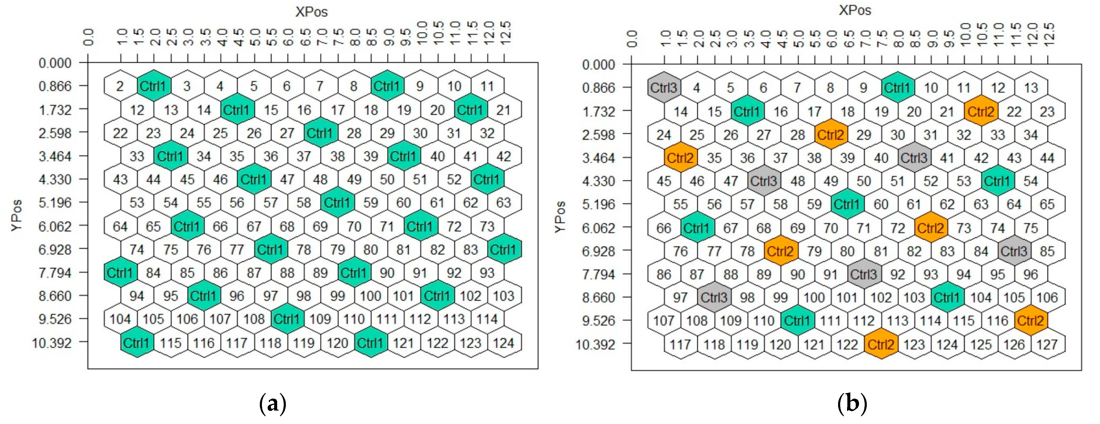
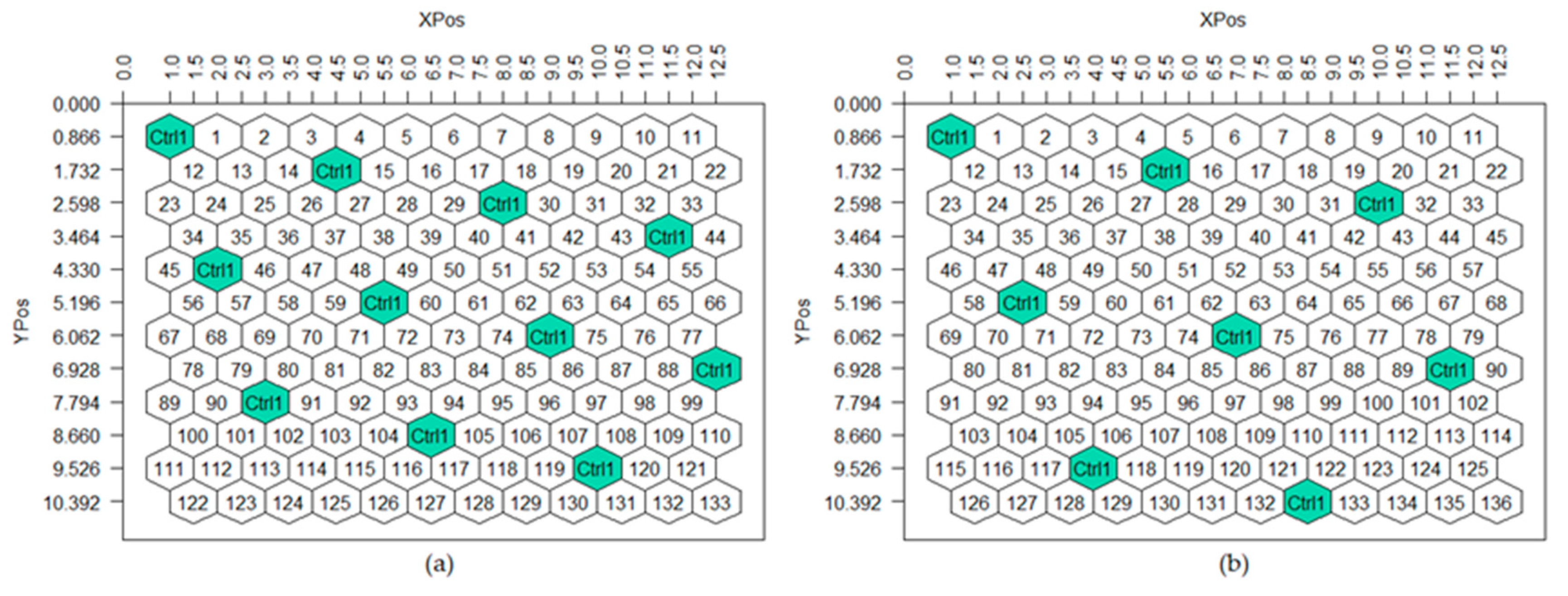
In a single-entry design (HSD0), plants are randomly allocated to the entire experimental area. Such a design may include either one (Figure 1a) or three (Figure 1b) entry-controls which are placed on specific plots and occupy one per seven experimental plots. The plots of an entry-control are determined by the K parameter (1, 3, 5 or 7). Different K values generate different control positions, however, neighboring positions of the same control always form an equilateral triangle, while their coordinates (X and Y) are equal to 2 and 1.

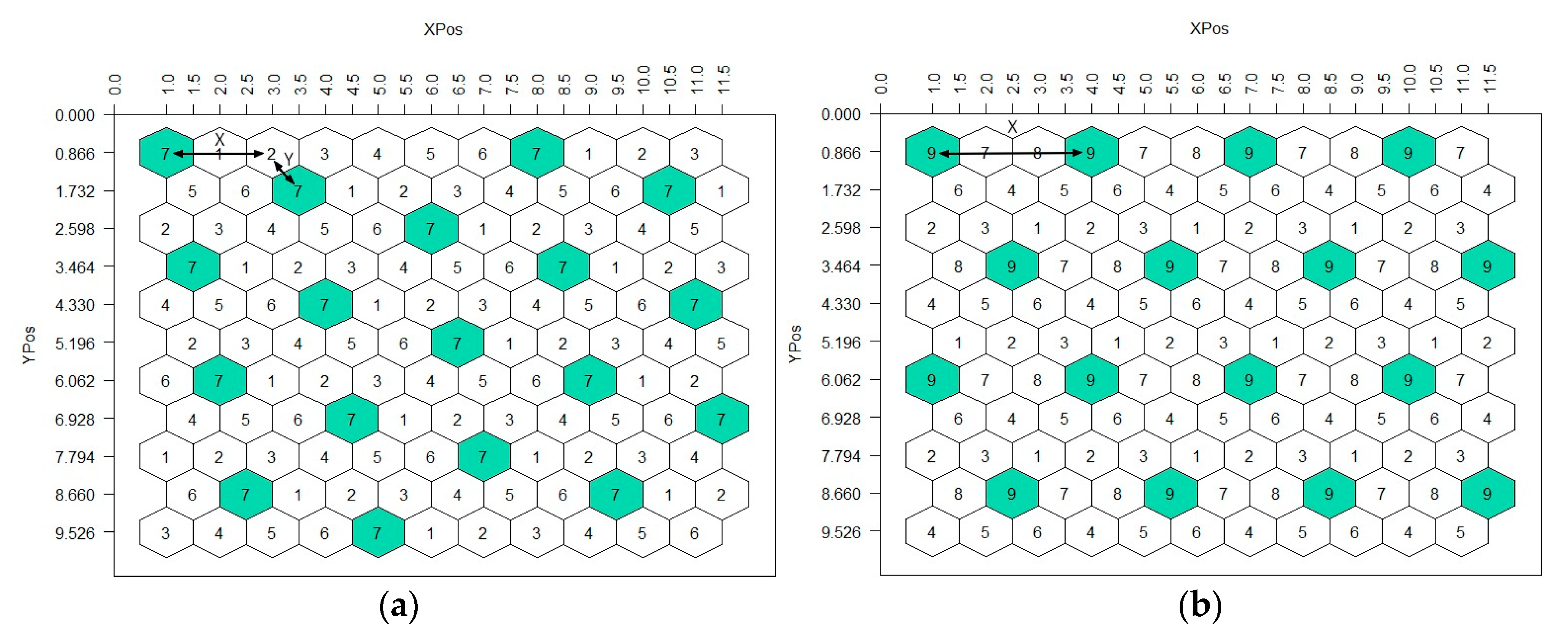
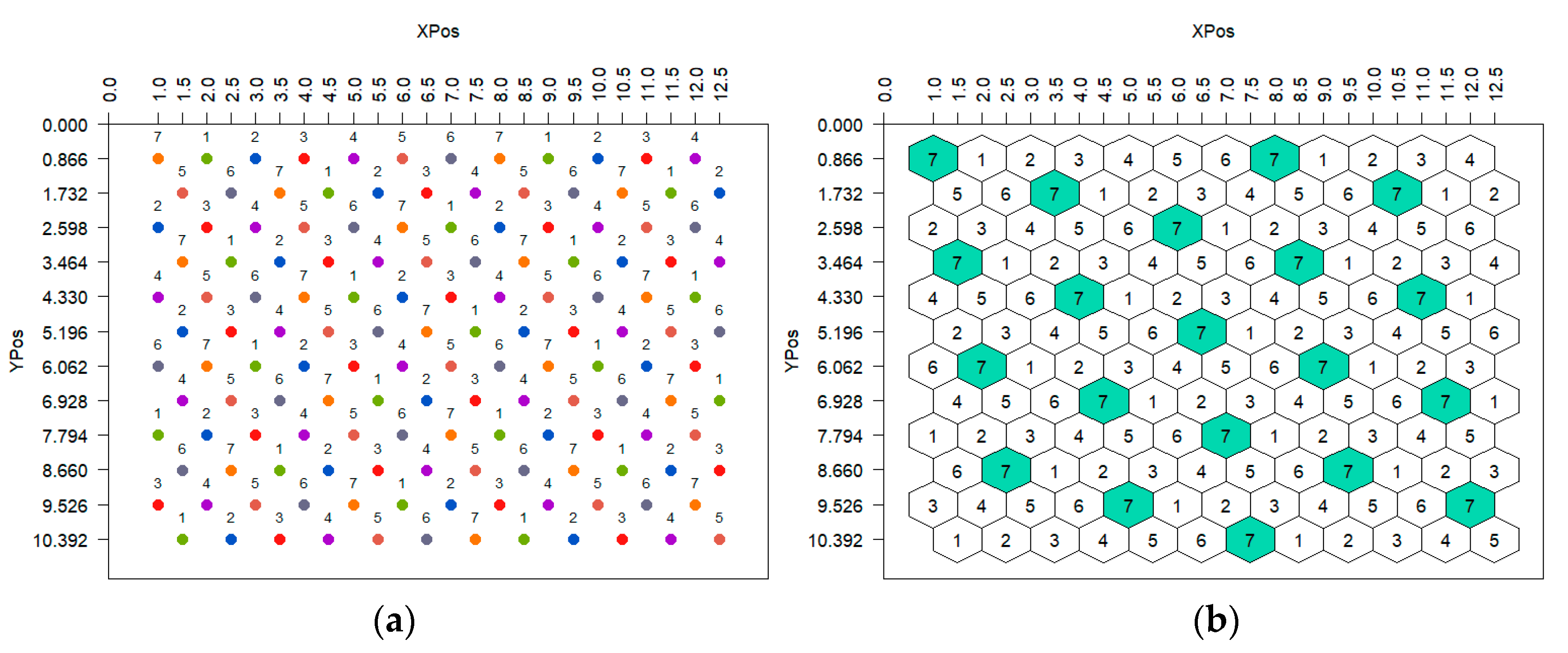
The multiple-entry designs, HSD(E), can be classified into two types, ungrouped and grouped. Ungrouped designs feature the entire set of entries in each row, arranged sequentially (Figure 2a). Grouped designs distribute the entries in groups across multiple rows (Figure 2b). The distinction between a grouped and ungrouped design can be determined by examining the numerical values of its X and Y coordinates. If the X and Y coordinates of the design do not share any common factors (divisors) other than 1, then the design is classified as ungrouped. Conversely, if a common factor (divisor) exists other than 1 between the X and Y coordinates, the design is classified as grouped. The common factor of the grouped designs determines the number of groups to which E is divided, whereas the ratio E/divisor determines the size m of groups. Furthermore, in both types of HSD(E) the coordinates X and Y indicate the distance in plant-to-plant steps (X-horizontal and Y-diagonal and vice versa) between the two nearest neighboring plants that belong to the same entry (Figure 2).

To construct an HSD(E), it is necessary to determine the initial entry code (number) for each field row. The initial number of each row is unique, specified by the parameter K_n (n = 1, 2, …, 6). The algorithms for calculating the parameters K_n and the initial number for each row are presented by Fasoulas and Fasoula [21]. Ungrouped designs have two constants (K₁ and K₂), whereas grouped designs have four constants (K₃, K₄, K₅ and K₆). For a particular HSD(E), the breeder chooses any of the corresponding K_n parameters. Although different K_n parameters generate different initial numbers resulting in different entry allocation, the principles of even and systematic entry arrangement are not disturbed.

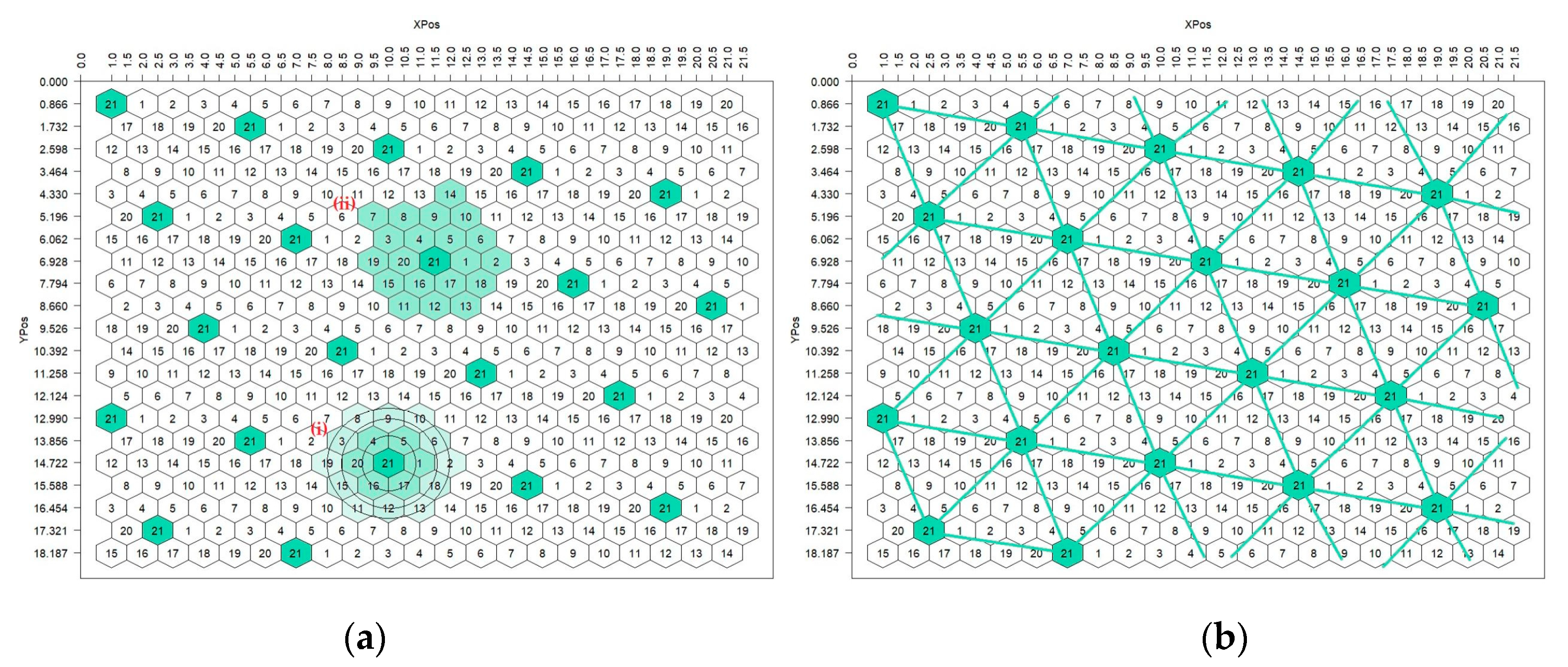
Generally, parameters Κ are used for the construction of HSDs. Any Κ of those available for a particular HSD arranges the entries evenly and systematically across the experimental area. In constructing of a particular HSD, different Κ values obviously result in different starting numbers of the rows. Still, in all resulting arrays, entries with similar numbers will form the characteristic equilateral triangle pattern (Figure 3b), and each entry will occur in the center of a moving, quasi-circular, and complete replicate [21]. In other words, different K values generate different entry positions, however, any entry is constantly surrounded by all the rest entries, i.e., occupies the center of a circular skeleton of a certain size that contains the entire set of entries, thus forming a complete circular block. Therefore, it does not matter which K the breeder will use to construct a particular HSD.

2.2. Analysis of a Honeycomb Selection Design

The HSD’s statistical analysis relies on the utilization of the circular moving ring. There are two types of moving ring. The commonly used one is a circle of flexible size, formed by the nearest neighboring plants according to their radius-distance from the central plant (Figure 3(ai)). The circle size is determined by the number of circumference plants which can vary from 6 to more than 120 plants. The breeder chooses a particular circle size, depending on the nature of entries and the experimental conditions. A larger circle is chosen when entries are highly heterogeneous (e.g., segregating progeny sister lines) and when there is high spatial heterogeneity or a high rate of missing plants in the experiment. The alternative type of moving ring is a circular skeleton of a certain size, since it contains the entire set of entries (Figure 3(aii)), thus forming a complete circular block. Due to the triangular pattern of entry allocation (Figure 3b), the moving ring, having a specific plant in the center, consistently covers the entire experimental area, thus constituting a block replication. This approach samples the spatial heterogeneity in the most efficient way to mitigate its obscuring effects. Hence, breeders can identify the outstanding entries and select the superior individual plants (genotypes) using the relevant indices and predictive equations [23].

The main selection criterion is the genotype’s ability to respond to resources. It is reflected by the grain yield per plant at the nil-competition regime, defined as Plant Yield Efficiency (PYE) [23]. The respective statistical measure, named PYE index, leverages the principle of the nearest neighbor adjustment corresponding to the squared relative yield of the central plant of the moving ring and is calculated by the equation:

$$PYE={(x/{\overline{x}}_r)}^2$$

(2)

where, x is the absolute yield of the central plant and ${\overline{x}}_r$ is the mean yield of the moving ring. Individual plants are ranked for their PYE values, while the average entry PYE (mPYE) is used to distinguish the most promising entries, and within high mPYE entries individual high PYE plants are selected.

Another selection criterion is the genotype’s ability to withstand the environmentally induced acquired plant-to-plant variation as a stability measure. It is approached by the entry Homeostasis Index (HI):

$$HI={(\overline{x}/s)}^2$$

(3)

where $\overline{x}$ and s denote the entry’s mean yield and standard deviation, respectively.

To apply single-plant selection, the breeder should focus on entries of high values in both mPYE and HI. However, it is recommended the HI is cautiously considered in early segregating generations due to genetic heterogeneity. The HI may undervalue a highly heterogeneous progeny sister line that reasonably would have a low HI value [24]. The breeder should focus exclusively on mPYE in highly heterogeneous entries.

Considering a plant for selection, its PYE and HI of the entry it belongs can be combined into a unique equation, the Plant Predictive Equation (PPE):

$$PPE=PYE·HI={{(x/{\overline{x}}_r)}^2·(\overline{x}/s)}^2$$

(4)

If the breeder wishes to combine the two indexes at the entry level, the mean Plant Predictive Equation (mPPE) is calculated, i.e., the average entry PPE value. In another option, the first part of Equation (4) is substituted by the Entry Yield Index (EYI) which is the squared relative entry mean yield $({\overline{x}/{\overline{x}}_t)}^2$, where ${\overline{x}}_t$ is the grand mean of the trial, resulting in the Entry Predictive Equation (EPE):

$$EPE=EYI·HI={({\overline{x}/{\overline{x}}_t)}^2·(\overline{x}/s)}^2$$

(5)

Entries are ranked in descending order of either mPPE or EPE to identify superior ones within which selection can be applied.

To establish a breeding program, the breeder may wish to evaluate several available germplasms, e.g., populations or landraces, to focus on the most promising ones as starting material [25,26]. For this particular purpose, germplasms are tested together in an HSD, including a homogeneous entry-control (e.g., an elite cultivar), having a special statistic tool developed for the first time to predict the response to single-plant selection, the Coefficient of Response to Selection (CRS):

$$CRS=({\overline{x}}_{sel}-{\overline{x}}_{contr})/s$$

(6)

where ${\overline{x}}_{sel}$ is the average yield of a predetermined number of selectable plants (those of the highest PYE) of the germplasm under consideration and $s$ is its standard deviation, while ${\overline{x}}_{contr}$ is the mean yield of an entry-control. The higher the CRS value of germplasm, the greater its potential to include superior genotypes.

3. Usage of the ‘rhoneycomb’ Package

The ‘rhoneycomb’ package comprises a set of functions intended to aid plant breeders in constructing and visualizing honeycomb selection designs, conducting statistical analysis on experimental data, and presenting the results. For developing the ‘rhoneycomb’ package, several open and free software, such as R and packages devtools, stats, utils and graphics have been used [27,28]. The package has been tested under Windows, Linux, and MacOS environments and is published in the Comprehensive R Archive Network (CRAN) at the link: https://cran.r-project.org/web/packages/rhoneycomb/index.html (accessed on 26 June 2023).

3.1. Installation of the Package

To install the ‘rhoneycomb’ package in R, the user executes the provided command within the R environment console:

• > install.packages(“rhoneycomb”)

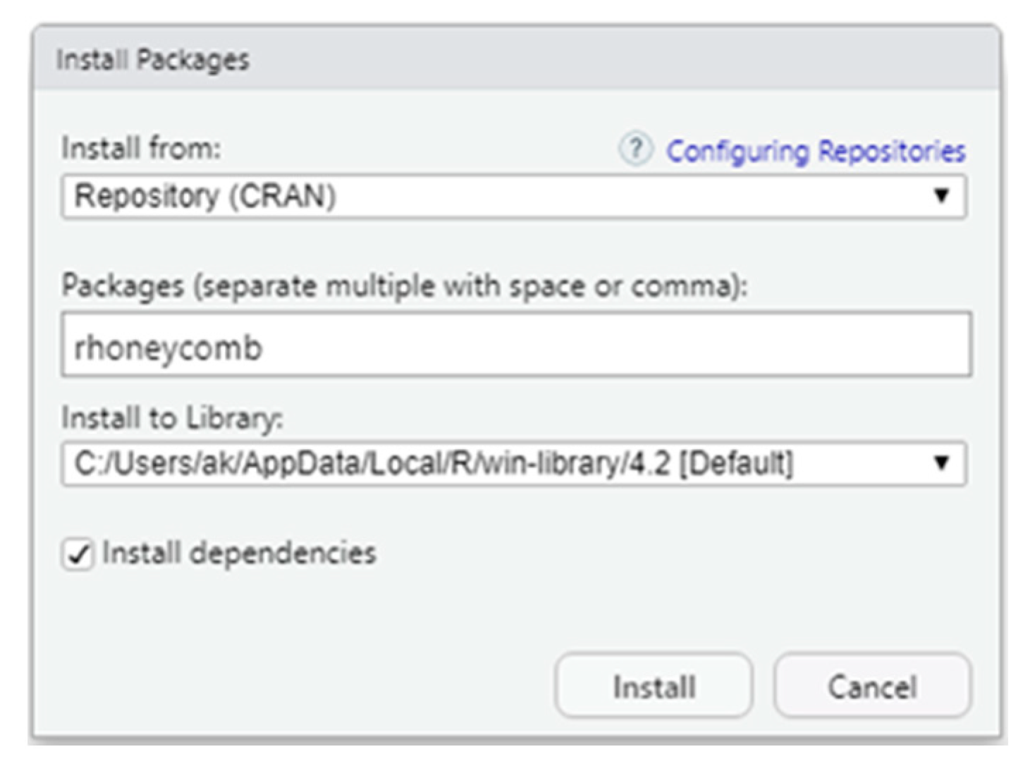
Alternatively, if the user uses the RStudio desktop, a friendly and comprehensive development environment for R [29], the package can be installed with the installer (Figure 4).

To start utilizing the package after installation, the user must load it into an R session by executing the following command.

• > library(rhoneycomb)

The package automatically checks for the required R packages (dependencies).

3.2. Generate Available Designs

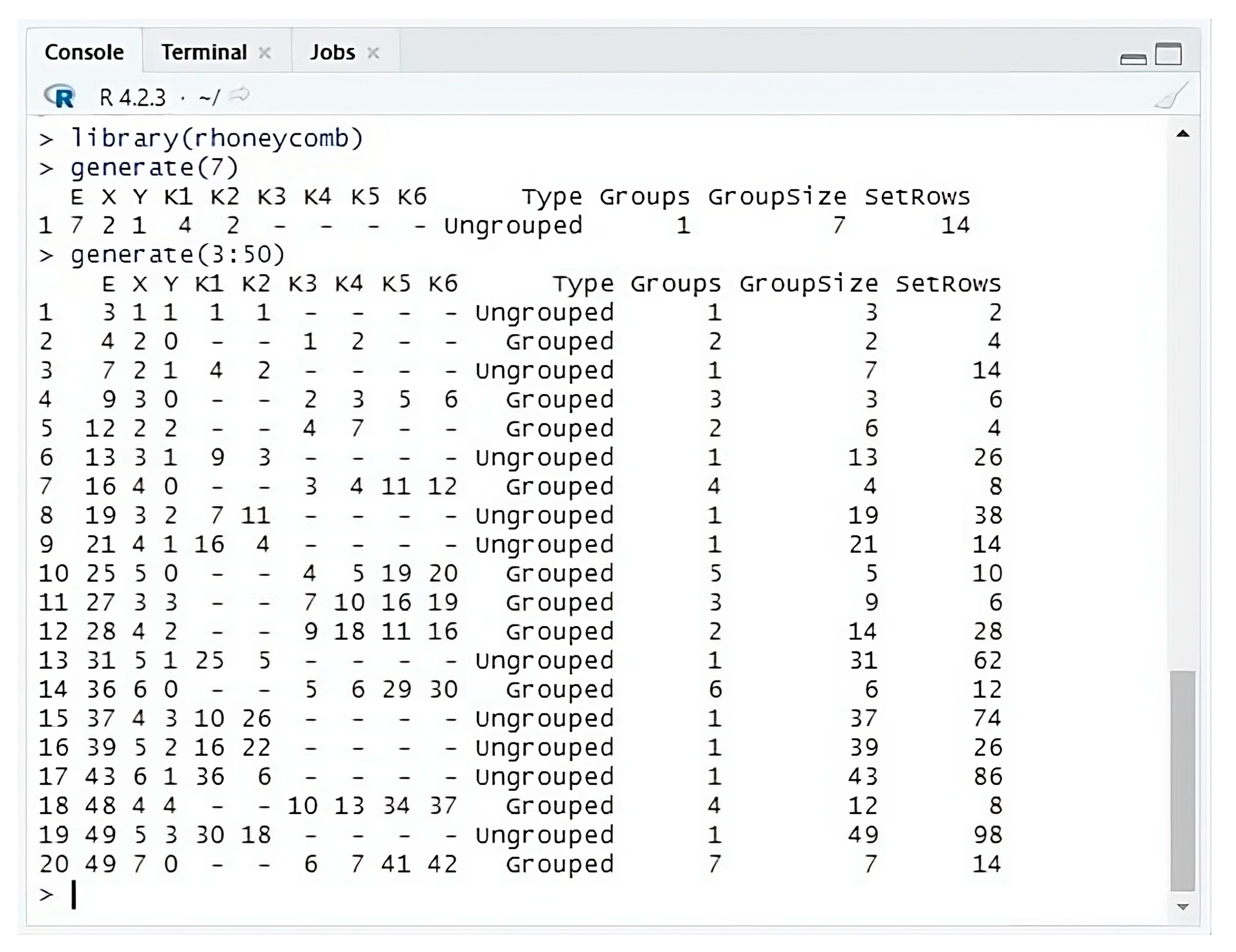
By implementing the algorithmic steps outlined in Fasoulas and Fasoula [21], the function generate() was developed. This function generates the essential parameters and features required to construct the HSD. Within the function, the E_gen argument is available to use. Users enter in the E_gen argument a single number or a vector of entries. To generate the parameters and features, for example for the HSD(7), the user executes the following command:

• > generate(7)

Alternatively, the user executes a command including a range of entries (e.g., 3 to 50 entries) to reveal the available designs:

• > generate(3:50)

These functions return a data frame with the available HSDs (number of entries E), the coordinates (X and Y) and $K_n$ parameters of the design, the type of the design (ungrouped or grouped), the number of groups (Groups), the size of the groups (GroupSize), and the number of rows (SetRows) required for one complete iteration of the design (Figure 5).

3.3. Construction and Visualization of Honeycomb Selection Designs

Four functions are available to facilitate the construction and visualization of honeycomb selection designs. The use of the appropriate function depends on whether the design includes one or more entries. The function for more than one entry is the HSD(). A user enters in the arguments of the HSD() function the number of entries being evaluated (E), the K parameter of the design (K), the number of rows (rows), the number of plants per row (plpr), the plant-to-plant distance in meters (distance) and the display of the HSD in polygons or points (poly = TRUE or FALSE). The first four arguments of the function must enter a value, while the last two (poly and control) are optional and default values are TRUE and FALSE, respectively. If the user enters a wrong number of entries or value of parameter K into the function or omits a required argument, the execution of the command leads to a warning message and appropriate instructions.

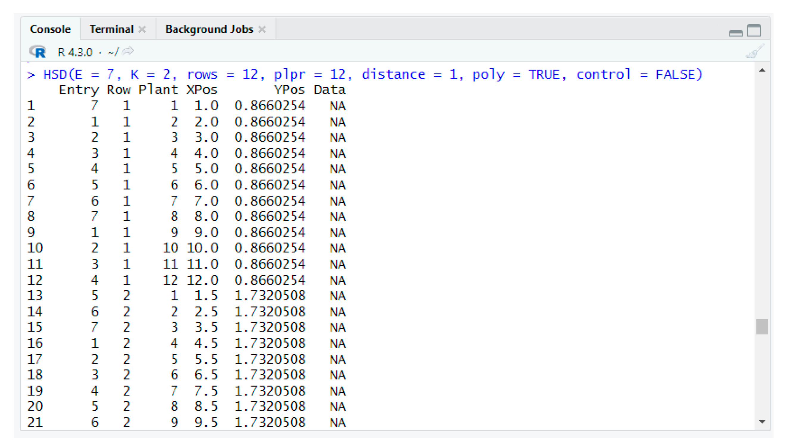
To construct the HSD(7) comprising 12 rows of 12 plants (total 144 plants), with planting distances of 1 m and parameter K = 2, the user executes the following command:

• > HSD(E = 7, K = 2, rows = 12, plpr = 12, d = 1, poly = TRUE, control = FALSE)΄
• or without the names of the arguments.
• > HSD(7, 2, 12, 12, 1)

The function returns the layout of the plants in the experimental field (Figure 6a,b). It also returns a data frame with six columns (Figure 7). The first column of the data frame represents the entries, the second column represents the rows of the design, the third column represents the position of the plant within the row, the fourth and fifth columns represent the planting distances, and the last column represents the yield data (at the moment empty). However, in designs with many plants, only a limited number of rows of the data frame are displayed in the command console. To display all the rows of the data frame, the user needs to increase the limit of max.print by changing the global options in R with the following command:

• > options(max.print = 10,000)

When the HSD evaluates a single entry, it could be combined with one or three additional entries used as controls. The function for a single-entry HSD without control, called HSD0(), does not require the input of the parameter K. The user enters in the HSD0() function the number of rows (rows), the number of plants per row (plpr), the plant-to-plant distance in meters (d), and the display of the design (poly = TRUE or FALSE). To construct a single-entry HSD comprising 12 rows of 12 plants (total 144 plants), with planting distances of 1 m, the user executes the following command:

• > HSD0(rows = 12, plpr = 12, d = 1, poly = TRUE)

The output of function HSD() includes both a data frame and a plot depicting the layout of plants in the experimental field.

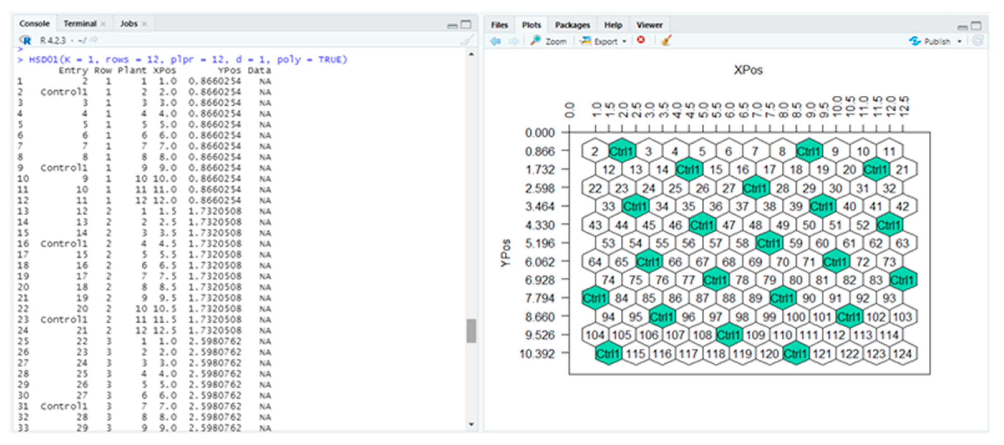
The other two functions corresponding to designs with one or three entry-controls are HSD01() and HSD03() and require the K parameter. To construct a single-entry HSD with one entry-control comprising 12 rows of 12 plants, with planting distance of 1 m and parameter K = 1, the user executes the following command:

• > HSD01(K = 1, rows = 12, plpr = 12, d = 1, poly = TRUE)

The HSD01() function returns a data frame and a plot with the layout of the plants in the experimental field (Figure 8).

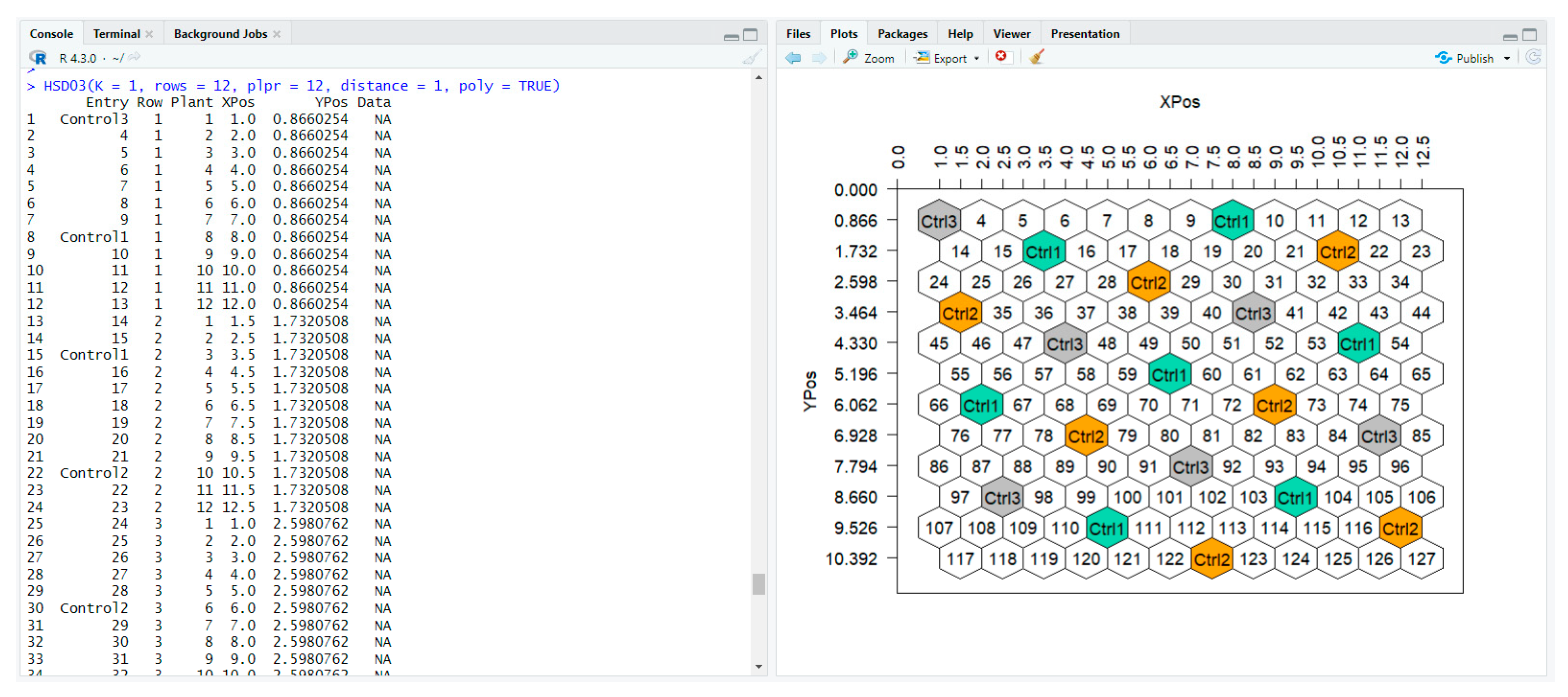
To construct a single-entry HSD with three entry-controls comprising 12 rows of 12 plants, with planting distances of 1 m and parameter K = 1, the user executes the following command:

• > HSD03(K = 1, rows = 12, plpr = 12, d = 1, poly = TRUE)

The HSD03() function returns a data frame and a plot with the layout of the plants in the experimental field (Figure 9).

Suppose plant breeders intend to evaluate the plants of a single entry with the addition of an entry-control, whose plants are more sparsely spaced than the standard control density; they should use the HSD() function with the control argument. In this case, the plant breeder will enter in the function HSD() the parameters of an HSD (recommended to be ungrouped) and, in the control argument, will declare TRUE. The result is a multiple-entry honeycomb arrangement, where all the positions correspond to plants of the single entry except those corresponding to the entry-control (that of the largest code number). The control plants are spaced according to the X and Y coordinates of the chosen HSD(E). For example, the control plants will occupy an area of the experimental field of approximately 7.5% if the HSD(13) is applied (X = 3 and Y = 1) (Figure 10a) and 5.5% in the case of the HSD(19) (X = 4 and Y = 1) (Figure 10b).

3.4. Import Experimental Data to Data Frame

The execution of the commands for constructing the HSD returns a data frame that includes an empty column for data input named Data. To import the data into the data frame, the user should first assign the data frame as an object and then input the data into a vector and assign it to the object. The experimental data are entered into a vector according to the order they appear in the data frame. If values are missing, they are replaced with the symbol NA.

The steps for constructing the HSD(4) with 4 rows and 4 plants per row and importing the data (16 observations, 2 of which are missing values) are as follows:

• Assign the data frame as an object named my_design.
• > my_design <- HSD(4,1,4,4,1)
• Data entry into the vector.
• > my_data <- c(5,8,7,NA,6,9,4,5,8,4,2,NA,6,8,4,5)
• Assign the data vector into the object.
• > my_design$Data <- my_data

To achieve the most efficient handling of the data frame regarding storage and editing, it is highly recommended to export it to spreadsheet files such as Excel or OpenDocuments using the commands of the package writexl [30]. Upon completing the data import into the spreadsheet file, the file can then be reimported into the R environment.

3.5. Analysis of Honeycomb Selection Designs

The analysis of the experimental data of any HSD is conducted by the function analysis() of the package. The function analysis() contains the arguments: Main_Data_Frame, Response_Vector, circle, blocks, row_element, plant_element and CRS. In order to perform the analysis, it is necessary to declare the first two arguments, while the remaining arguments can be optionally declared. In the argument Main_Data_Frame, the user enters the assigned object data frame generated by one of the functions HSD(), HSD0(), HSD01() and HSD03(), and in the argument Response Vector, the vector of the data column.

The function defaults to the six nearest neighboring plants if the user does not set a specific circle size. Alternatively, instead of circles, the user can use the complete circular block, the moving ring that contains all nearest neighboring entries. In this case, the block argument should be declared as TRUE. To locate the circle or the complete circular block surrounding a specific plant, the user declares in the argument row element the row number of the plant and, in the argument plant element, the position of the plant in the row. In addition, the user can declare the number of selected plants used to calculate the CRS, considering the entry with the highest identification number as the control.

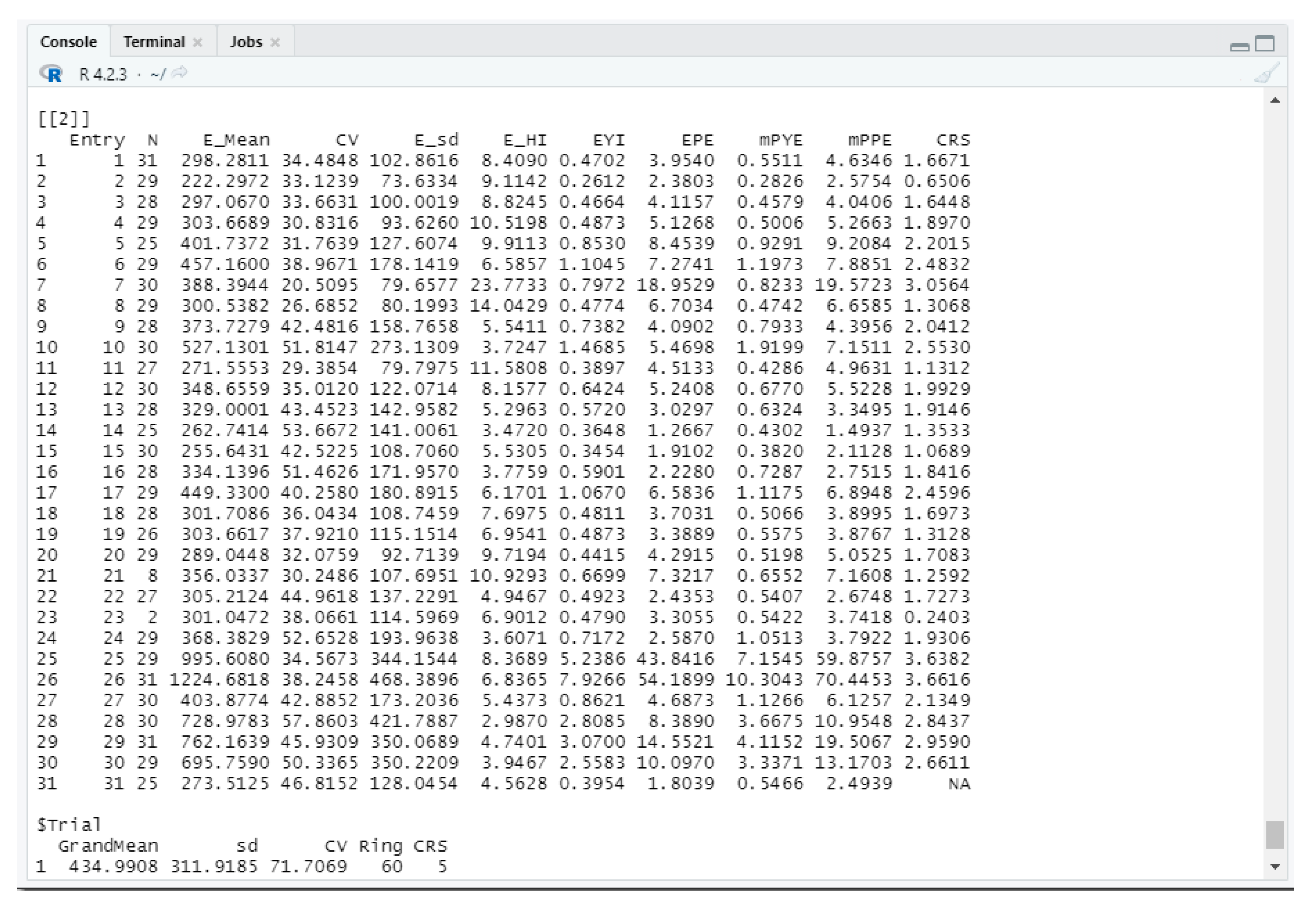
The function analysis() returns two data frames. The first data frame presents for each plant the following: yield, moving ring size, moving ring mean, PYE value, entry mean, entry number of plants, entry standard deviation, entry HI, and PPE value. The second data frame presents for each entry: number of plants, mean yield, Coefficient of Variation (CV%), standard deviation, HI value, ΕYI value, ΕPE value, mPYE value, mPPE value, and CRS value. The function also returns the descriptive statistics of the trial (grand mean, standard deviation, and CV%), the size of the moving ring, and the number of selected plants used to calculate the CRS.

4. Illustrative Examples

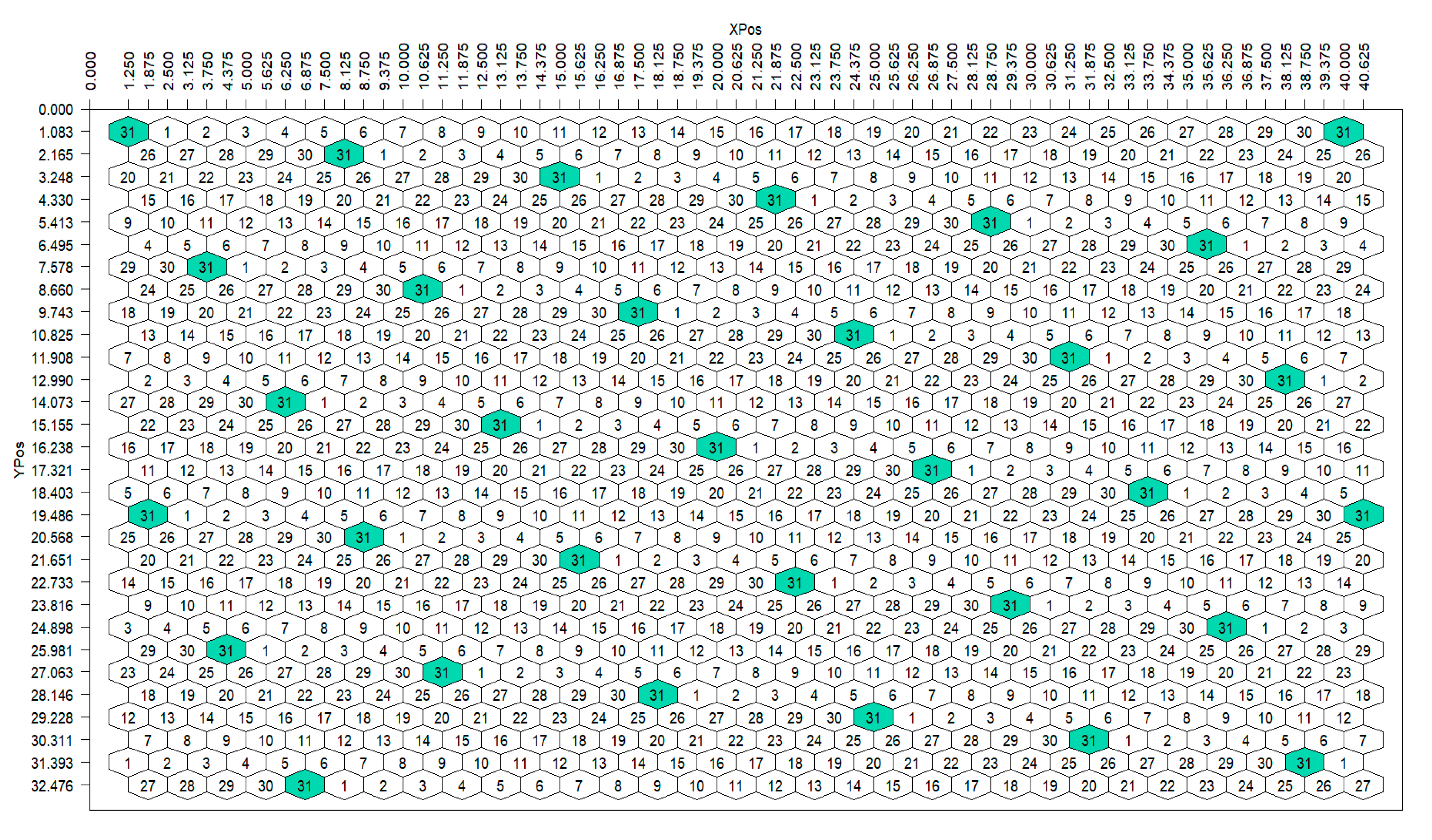
The following example is a showcase for the construction and analysis of the HSD. The HSD(31) trial included 31 maize lines and was conducted in 2012 on the farm of the Technological Education Institute of Western Macedonia in Florina, Greece [31]. For construction and analysis, the parameter K = 5 was used. The experiment consisted of 30 rows and 32 plants per row (960 total plants), while the planting distance was 1.25 m. To construct the design, the user must initially select the design parameters by executing the function generate(31). Then, for the construction of the HSD(31), the command will be executed:

• > FLORINA <- HSD(E = 31, K = 5, rows = 30, plpr = 32, d = 1.25, poly = TRUE, control = FALSE)

This command will return the plot with the layout of the plants (Figure 11).

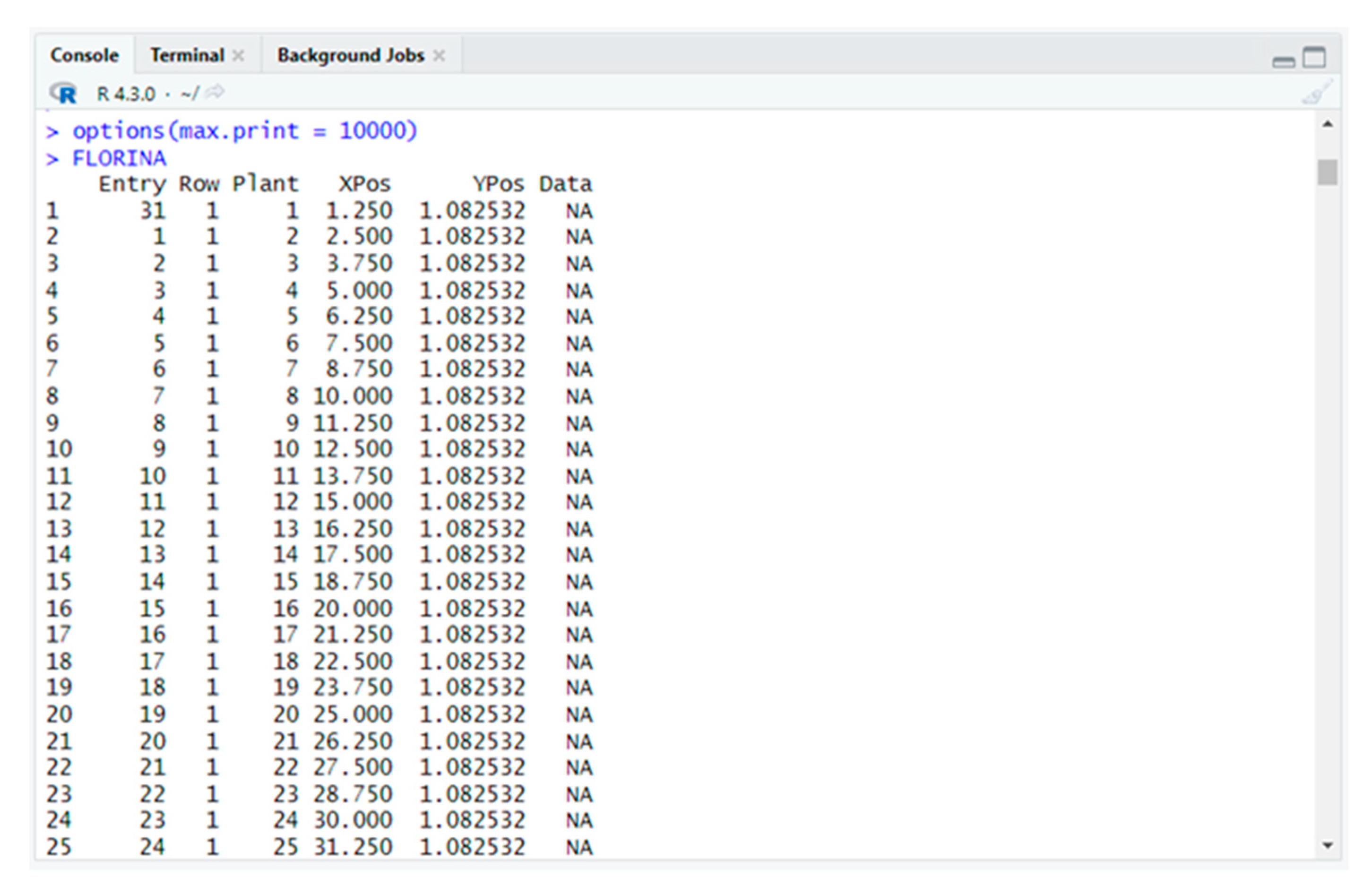
By executing the object of the above command (FLORINA), the data frame will be displayed (Figure 12).

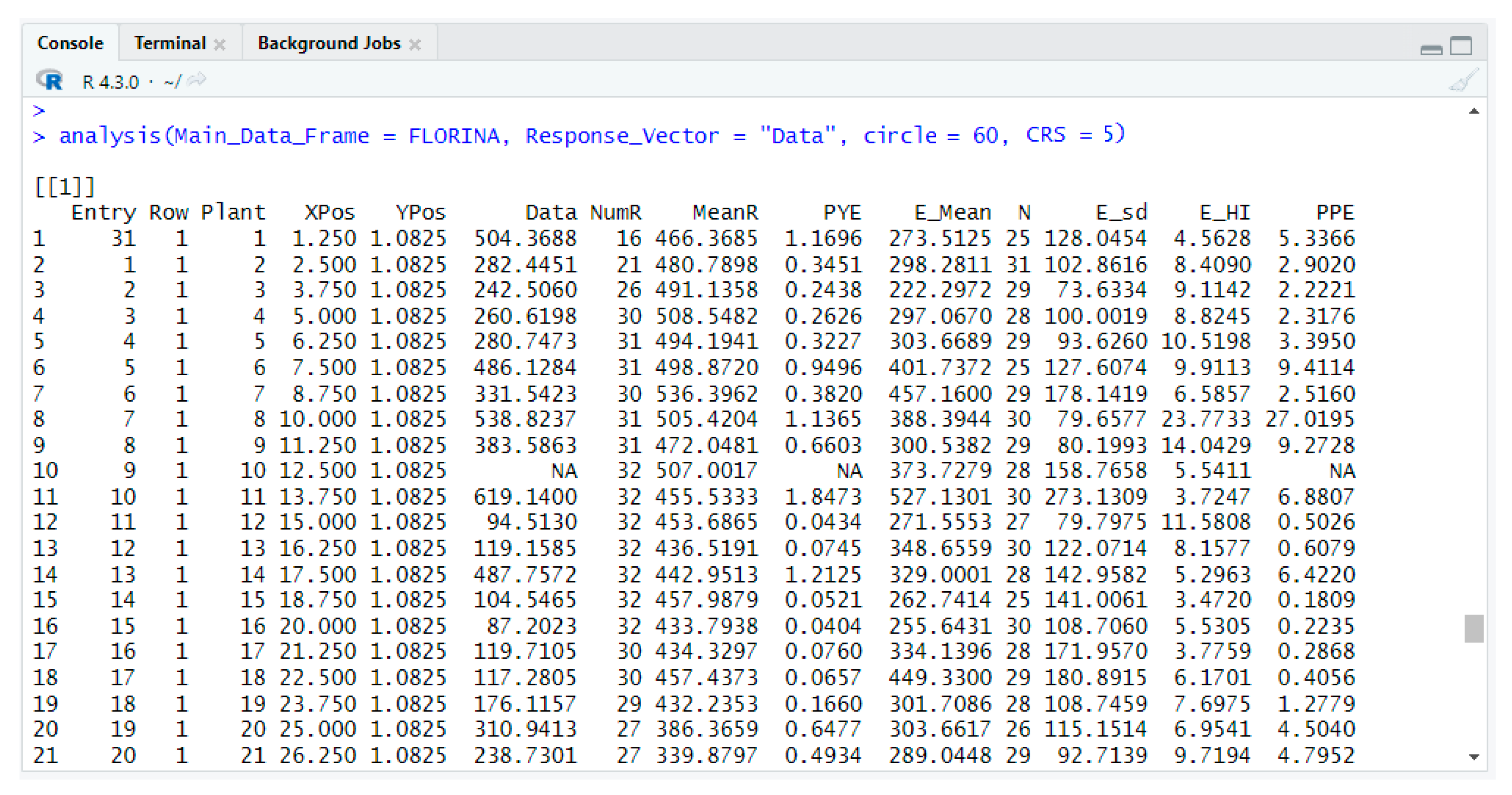
Data can be added to the data frame either by directly using a data vector or by exporting the dataset to a spreadsheet and then importing the data. The analysis of the data is performed by executing the function analysis(), specifying the name of the dataset (e.g., FLORINA), the data column (Data), the circle size (60 plants), as well as the number of selected plants for the CRS (the 5 plants of the highest PYE):

• > analysis(Main_Data_Frame = FLORINA, Response_Vector = "Data", circle = 60, CRS = 5)

The function analysis() returns two data frames, one for the evaluation of individual plants (Figure 13) and one for the evaluation of the entries (Figure 14).

From the first data frame, the plant breeder ranks the plants in descending order based on the plant yield efficient index (PYE).

From the second data frame, the plant breeder ranks the entries in descending order based on one of the following measures, depending on their nature (highly heterogeneous or fairly homogeneous): yield performance (mean or EYI or mPYE), stability (HI), combined yield and stability (EPE or mPPE). Single-plant selection for high PYE (the first data frame) applies within the top entries. If experimentation focuses on evaluating germplasms as potential starting material for breeding, entries of the second frame are ranked on the Coefficient of Response to Selection (CRS). In the present example, CRS values were calculated using entry 31 as the control.

5. Conclusions

This paper gives a detailed presentation of the upgraded version of the ‘rhoneycomb’, a free and open-source R package comprising functions that can enhance the construction, visualization, and analysis of HSDs for plant breeders, providing them with a more precise and user-friendly approach. The upgraded package offers additional functions and input options to customize further their research aims. The functionalities provided by the ‘rhoneycomb’ package enable the selection of high-yielding genotypes and ensure stability in trait performance. These functionalities increase efficiency and speed, aid the mechanization of the early stages of plant selection, and serve as a valuable contribution to the crop breeding community, offering efficient assistance in the initial stages of a breeding program. Thus, the proposed new version of the package can greatly impact crop breeding programs by making the selection of superior plants more efficient and reliable. The package is free to download at CRAN: https://cran.r-project.org/web/packages/rhoneycomb/ (accessed on 26 June 2023) with additional examples and information.