
In-Season Crop Type Detection by Combing Sentinel-1A and Sentinel-2 Imagery Based on the CNN Model

1
Law School, Panzhihua University, Panzhihua 617000, China
2
State Key Laboratory of Efficient Utilization of Arid and Semi-arid Arable Land in Northern China, the Institute of Agricultural Resources and Regional Planning, Chinese Academy of Agricultural Sciences, Beijing 100081, China
3
School of Geographical Sciences, China West Normal University, Nanchong 637009, China
4
Guokechuang (Beijing) Information Technology Co., Ltd., Beijing 100070, China
*
Author to whom correspondence should be addressed.
Agronomy 2023, 13(7), 1723; https://doi.org/10.3390/agronomy13071723
Submission received: 1 June 2023
/
Revised: 22 June 2023
/
Accepted: 25 June 2023
/
Published: 27 June 2023
(This article belongs to the Special Issue Art of Spectra: At the Crossroad of Agriculture and Remote Sensing Disciplines)
Abstract
:In-season crop-type maps are required for a variety of agricultural monitoring and decision-making applications. The earlier the crop type maps of the current growing season are obtained, the more beneficial it is for agricultural decision-making and management. With the availability of a large amount of high spatiotemporal resolution remote sensing data, different data sources are expected to increase the frequency of data acquisition, which can provide more information in the early season. To explore the potential of integrating different data sources, a Dual-1DCNN algorithm was built based on the CNN model in this study. Moreover, an incremental training method was used to attain the network on each data acquisition date and obtain the best detection date for each crop type in the early season. A case study for Hengshui City in China was conducted using time series of Sentinel-1A (S1A) and Sentinel-2 (S2) attained in 2019. To verify this method, the classical methods support vector machine (SVM), random forest (RF), and Mono-1DCNN were implemented. The input for SVM and RF was S1A and S2 data, and the input for Mono-1DCNN was S2 data. The results demonstrated the following: (1) Dual-1DCNN achieved an overall accuracy above 85% at the earliest time.; (2) all four types of models achieved high accuracy (F1s were greater than 90%) on summer maize after sowing one month later; (3) for cotton and common yam rhizomes, Dual-1DCNN performed best, with its F1 reaching 85% within 2 months after cotton sowing, 15 days, 20 days, and 45 days ahead of Mono-1DCNN, SVM, and RF, respectively, and its extraction of the common yam rhizome was achieved 1–2 months earlier than other methods within the acceptable accuracy. These results confirmed that Dual-1DCNN offered significant potential in the in-season detection of crop types.
1. Introduction
Crop-type mapping is an important component of agricultural monitoring and management. In-season crop-type information is required for a variety of monitoring and decision-making applications, such as yield estimation, agricultural disaster assessment, and crop rotation, which is important for food security [1,2]. The earlier the crop type maps of the current growing season are obtained, the more beneficial it is for agricultural decision-making and management. Remote-sensing technologies have greatly improved crop-type mapping for decades at the regional to continental scale [3,4,5,6]. Multi-temporal data have proved effective for crop-type mapping given that the phenological evolution of each crop produces a unique temporal profile of reflectance or radar-backscattering coefficient [7,8]. Early detection of crop types, however, remains challenging in agricultural remote-sensing monitoring because it needs to extract distinguishable features from the limited data in the early season. Moreover, for landscapes dominated by smallholder agriculture, such as those in China, with characteristics of complex cropping patterns and a high degree of land fragmentation, the timely and accurate mapping of crop types represents an especially challenging task [9,10,11].
The launch of optical and synthetic aperture radar (SAR) remote-sensing satellites with high spatial and temporal resolutions, such as Sentinel-1A/B (S1) and Sentinel-2A/B (S2) in the European Copernicus project [12], provides more opportunities for early crop-type detection [13]. S1 and S2 can provide SAR and optical (multispectral) images, respectively, at 10 m spatial and 5-day (S2) or 6-day (S1) temporal resolutions. The integration and application of the two types of data hold great significance for improving the accuracy of early crop-type detection. First, the wealth of crop phenology information from dense time series data (TSD) can be used to identify different crop types with the same spectrum [14,15]. Second, compared with single-source remote-sensing data, multisource data have a higher time frequency of data acquisition, which directly improves timeliness. Third, different sensors have different degrees of sensitivity to crop parameters, and optical data can be used to estimate crop chemical components, such as chlorophyll and water [16]; additionally, SAR data are more sensitive to crop structure (e.g., height, porosity, coverage) and field conditions (e.g., field moisture content) [17]. Understanding how to effectively combine the complementary information of S1 and S2, however, remains a challenge in the field of in-season mapping.
At present, in mainstream machine learning (ML) approaches, such as support vector machine (SVM) and random forest (RF), the sequential relationship of time series imagery is not clearly considered, which means that we might ignore some useful information during crop-type detection [18,19]. In recent years, as a breakthrough technology in ML, deep learning (DL) has shown great potential in the field of remote-sensing information extraction [20,21,22]. Among DL models, recurrent neural networks (RNNs) and convolutional neural networks (CNNs) have demonstrated unprecedented performance in the extraction of temporal features [23,24]. Long short-term memory (LSTM) and gated recurrent unit RNNs (GRU) [25] are variants of the RNN unit that solve the problem of gradient disappearance or explosion seen with an increasing time series.
In crop-type mapping, these models have been explored mainly by using single-source data, such as microwave data [11,18,26], optical data (or vegetation index) [15,19], or by filling gaps in optical images by converting SAR data to the normalized difference vegetation index (NDVI) using a hybrid architecture of CNN and LSTM [27]. These methods are not available for multisource data because the sequence length and time interval of different spectral bands (or polarization characteristics) of single-source time series are the same; meanwhile, the time series from different sources usually have different sequence lengths and time intervals. In addition, although Ienco et al. [28] proposed an architecture based on the GRU and CNN to boost the land cover classification task by combining S1 and S2 images, their method is not exercisable for the task of in-season detection of crop types. The main reason for this is that compared with CNNs, RNNs have more parameters determined by the length of the time series [29]. Different time series are usually input into architectures to find the best date, and therefore, if there are many parameters in DL architectures, the training becomes time-consuming, especially for long time series.
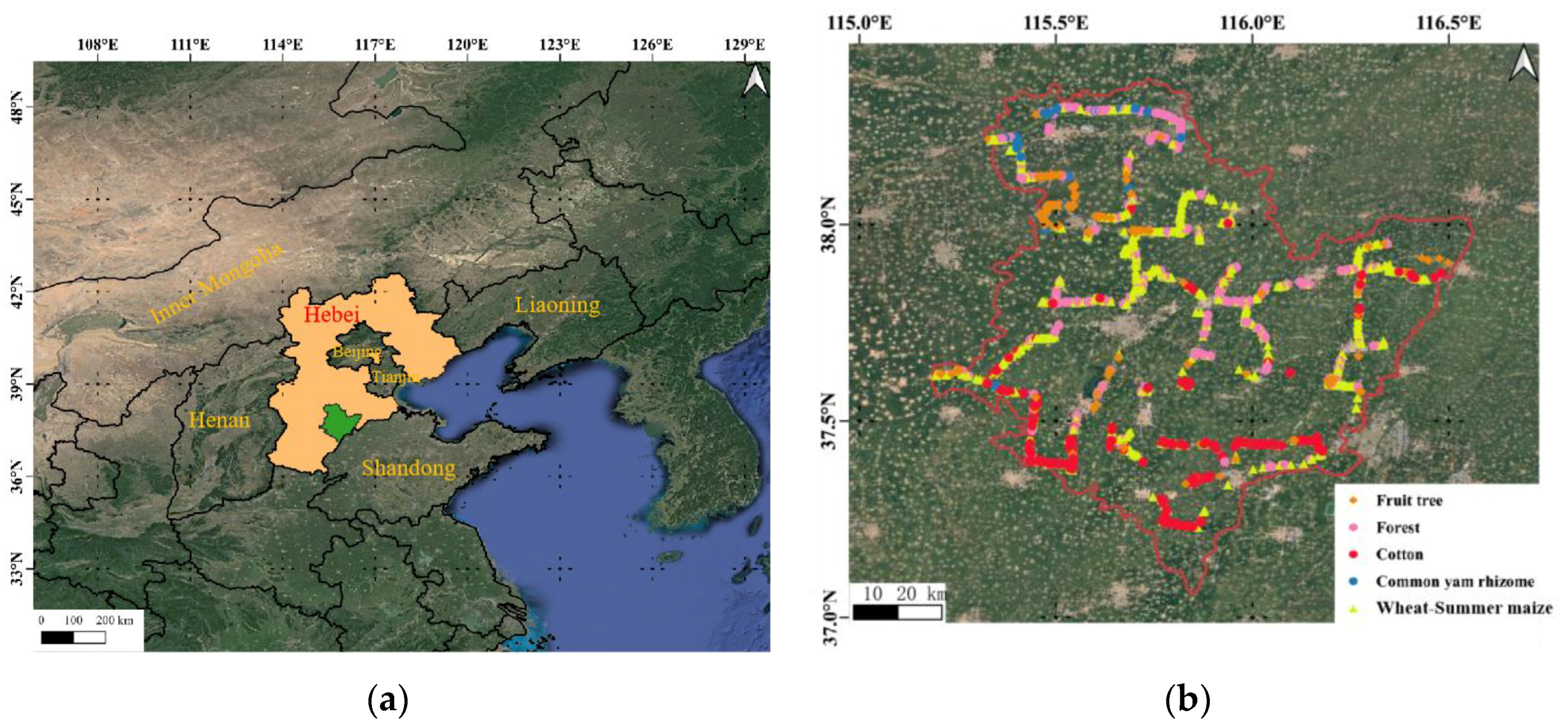
In a previous work [11], we evaluated CNNs, LSTM RNNs, and GRU RNNs for early crop-type classification using S1A time series data. Results confirmed that the training of CNNs used less time, and CNNs performed better for evenly distributed time series signals. In the present work, we described an architecture based on the CNN (called Dual-1DCNN) to integrate the time series data of S1A and S2 and used an incremental training method to attain the network on each data acquisition date. The aim of the Dual-1DCNN architecture is to improve early crop-type detection by taking advantage of S1A and S2 from three levels: (1) ensuring that more information can be used in the early season; (2) complementing sensitivities of optical and radar data for different parameters; and (3) improving the timeliness of detection by having more data acquisition dates. We conducted a case study for Hengshui City (Figure 1a), a main cropping city in northern China.
2. Materials
2.1. Study Site
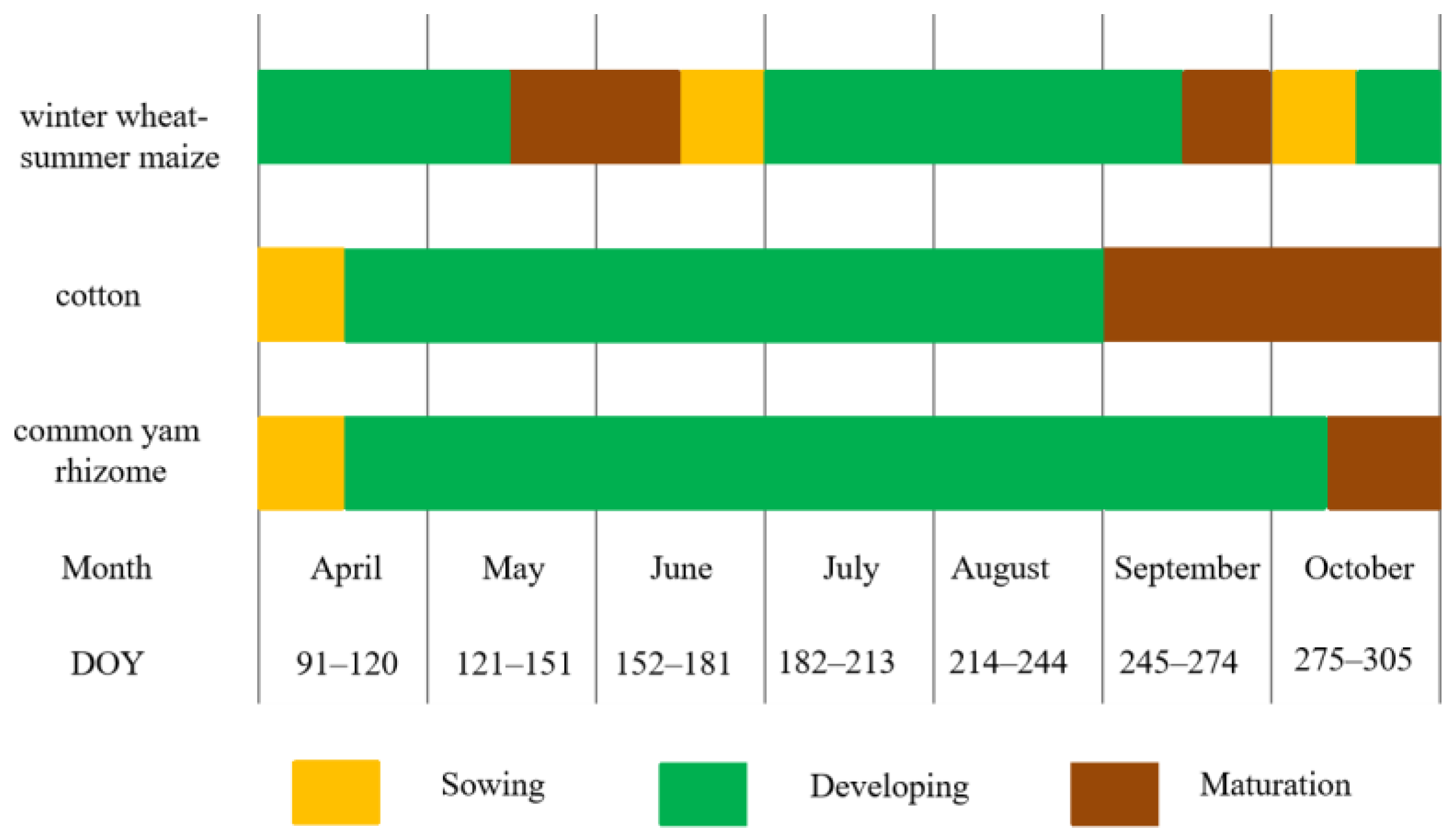
Hebei Province is a main cropping province located in northern China. Hengshui City occupies an area of 8815 km2 (Figure 1b) and is located at an elevation of 24.19 m above sea level. Hengshui has a mid-latitude steppe climate and the district’s yearly temperature is 14.04 °C, which is −0.58% lower than China’s average. Hengshui typically receives about 109.65 mm of precipitation and has 161.37 rainy days (44.21% of the time) annually. It is a typical wheat–maize rotation area and its main economic crops are cotton, common yam rhizome, fruit trees, and vegetables. The growing season for winter wheat is from early October to the middle of the following June, and summer maize is planted at the end of the winter wheat season and harvested in late September. The growing seasons of cotton and common yam rhizome are from late April to the end of October and early April to the end of October, respectively. The growth periods of fruit trees generally last all year. In this study, we categorized the phenology of summer maize, cotton, and common yam rhizome into three periods: sowing, developing, and maturation. The details of these periods are shown in Figure 2.
2.2. Ground Reference Data
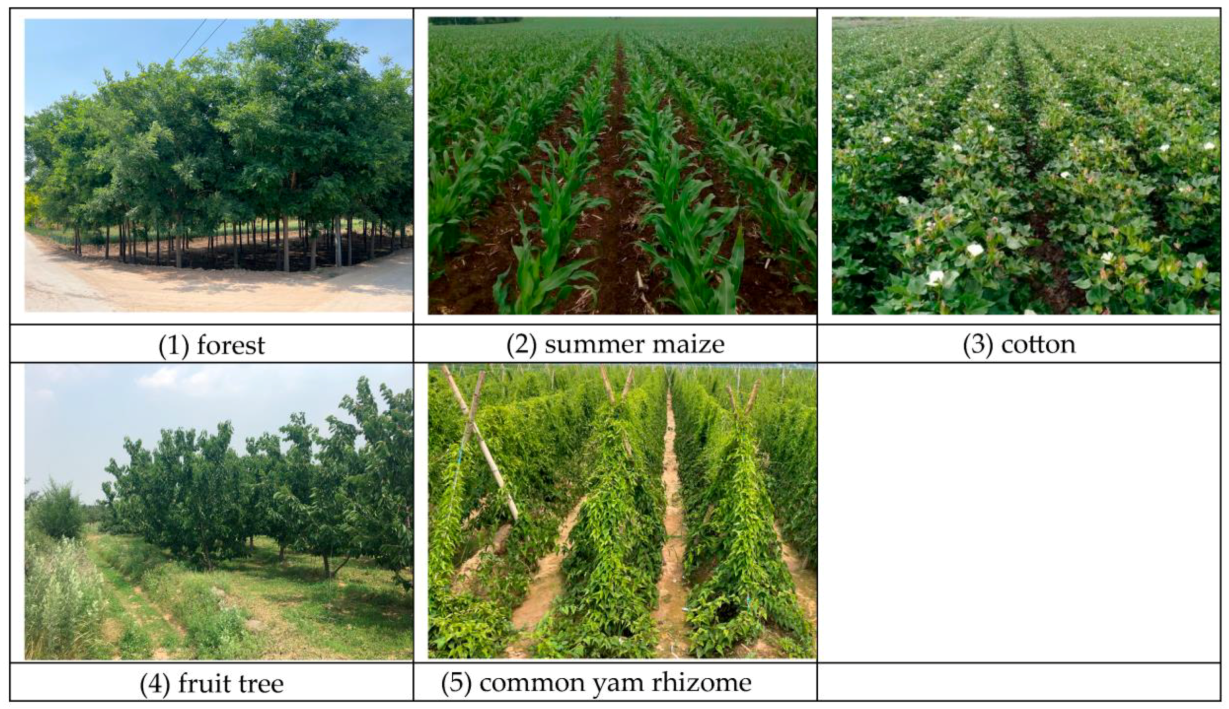
A field investigation in the study area was conducted in July 2019, when the main summer crops were in their reproductive period as shown in Figure 3. To obtain sampling points distributed across the entire region, we designed a sampling route based on expert knowledge and recorded the main crop types and corresponding geographic coordinates on the route. A total of 1186 samples from the field survey were acquired. Afterward, 756 samples were taken by manual interpretation from the surveyed parcels on the platform Google Earth Map. Therefore, a total of 1942 sample points for five main types of local vegetation in the summer season: (1) forest, (2) summer maize, (3) cotton, (4) fruit tree, and (5) common yam rhizome were used in this study. The distribution of the number of samples per type is shown in Table 1, and the calendars are expressed in Figure 2. All geographic coordinates of samples were re-projected to WGS 84/UTM zone 50 N.
2.3. Sentinel-1A/2 Data and Preprocessing
The S1A and S2 data were downloaded from the European Space Agency (ESA) Sentinels Scientific Data Hub website. The Interferometric Wide Swath (IW) Ground Range Detected (GRD) product of S1A was used in this study. This product with 10-m resolution contained both VH and VV polarizations and had a 12-day revisit time. The S2 (Level-1C) product included blue, green, red, and near-infrared 1 (NIR1) bands at 10 m; red edge (RE) 1 to 3, NIR2, and shortwave infrared 1 (SWIR1) and SWIR2 at 20 m; and three atmospheric bands (band 1, band 9, and band 10) at 60 m. For this study, the three atmospheric bands were not used because they were dedicated to atmospheric corrections and cloud screening the three atmospheric bands [11]. There were 15 S1A mosaic images and 35 S2 mosaic images over Hengshui from day of year (DOY) 103 to 273 (13 April to 30 September) 2019. Note that DOY 273 was at the late season of the three crop types, and we used the data before DOY 273, which met the requirements of early crop-type detection.
We preprocessed the S1A data in the Sentinel Application Platform (SNAP) open-source software version 7.0.2. The preprocessing stages included (1) radiometric calibration; (2) speckle filtering, in which case we applied the Gamma-MAP (maximum a posteriori) speckle filter with a 7 × 7 window size to all images to remove the granular noise; (3) orthorectification, for which we applied range Doppler terrain orthorectification to the images; and (4) re-projection, for which we projected the orthorectified SAR image to the Universal Transverse Mercator (UTM) coordinate system, Zone 50 North, World Geodetic System (WGS) 84.
The preprocessing stages for the S2 images were as follows:
- (1)
- Atmosphere calibration: We used the sen2cor plugin v2.5.5 to process reflectance images from Top-of-Atmosphere (TOA) Level 1C S2, to Bottom-of-Atmosphere (BOA) Level 2A, following Sentinel-2 for Agriculture (Sen2-Agri) protocols [30] (http://www.esa-sen2agri.org/, accessed on 24 November 2020).
- (2)
- Masking clouds: We used Function of mask (Fmask) 4.0 [31] to mask clouds and cloud shadow (the cloud probability threshold was set to 50%). Note that compared with cloud confidence layers in the output of sen2cor, Fmask 4.0 results were more accurate in our study area.
- (3)
- Resampling: We resampled the images of RE1, RE2, RE3, NIR2, SWIR1, and SWIR2 from step (1) and cloud masks from step (2) to 10 m.
- (4)
- Filling gaps: Because linear interpolation is usually appropriate for short gaps [32], we adopted the Savitzky–Golay filter to reconstruct each band value using a moving window of seven observations and a filter order of 2 [33]. Note that we used S-2A/B images observed in March and October 2019 because of missing values in early April and late September.
3. Methodology and Experiments
3.1. CNN for Multivariate
The four main types of layers in the CNN architecture are the convolutional (Conv) layer, rectified linear unit (ReLU) layer, pooling layer, and fully connected (FC) layer [34]. For classification tasks, CNNs are typically composed of various combinations of these four types followed by a softmax logistic regression layer, which acts as a classifier that produces the predictive probabilities of all the object categories in the input data [35,36]. Moreover, it is common to incorporate some other components, such as dropout and batch normalization (BN) [37], into CNN architectures to improve their generalization ability and prevent overfitting.
The one-dimensional CNN (1D CNN) is a special form of CNN, and it employs a 1D convolution kernel to capture the temporal pattern or shape of the input series [38]. The Conv layer of 1D CNN is usually expressed as Conv1D. The convolutional operation is actually the dot products between kernels and local regions of the input. A basic 1D convolutional block always consists of a Conv1D layer followed by a ReLU layer. We expressed a multivariate time series with variables of length as , where denotes the t-th observations of all variables, represents the value of the d-th variable of , and . Here, all variables had the same . For illustrative purposes, we assumed kernels for all Conv1D layers; however, different kernel sizes also could be assigned if desired. Considering L Conv1D layers, the kernels for each Conv1D layer were parameterized by tensor and biases , where . For the l-th layer, the i-th component of the activation can be calculated by the following function:
where is from the previous layer and Conv1D (…) is a regular 1D convolution without zero padding on the boundaries.
3.2. The Dual-1DCNN
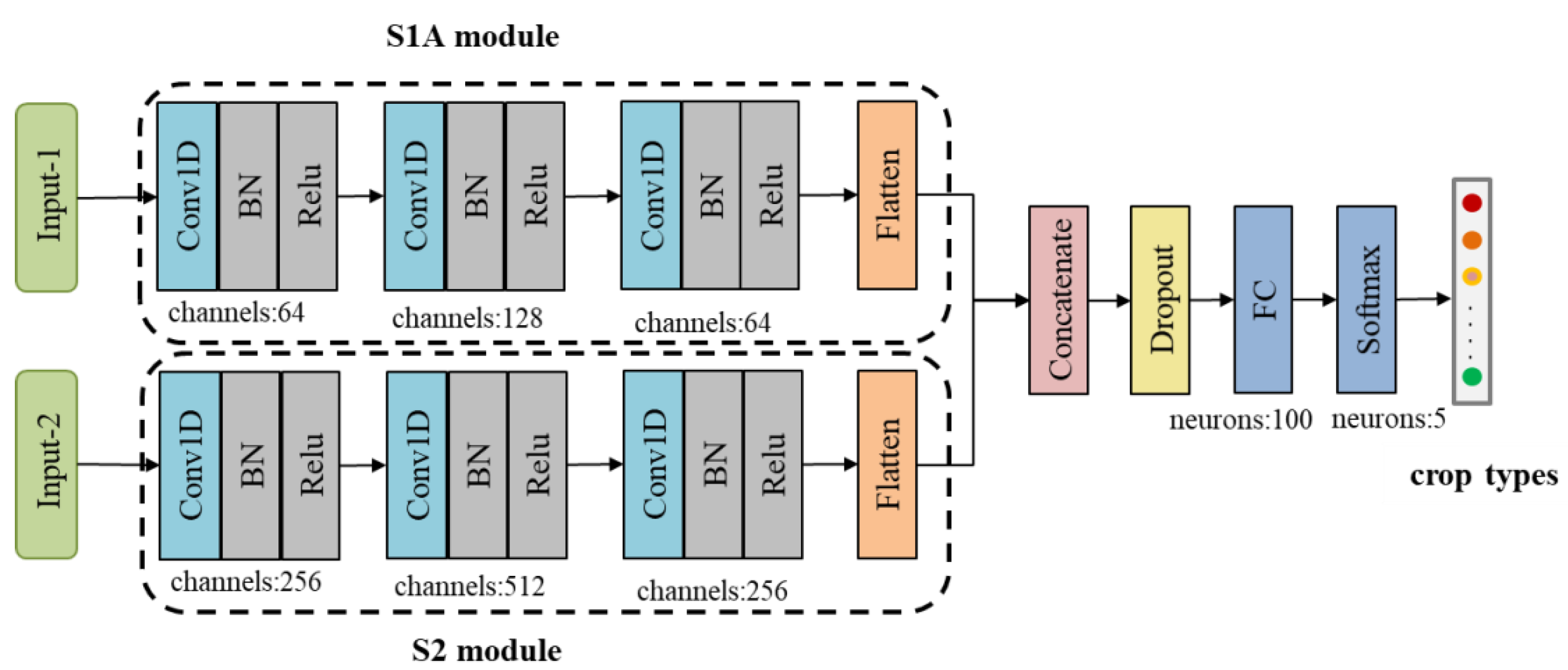
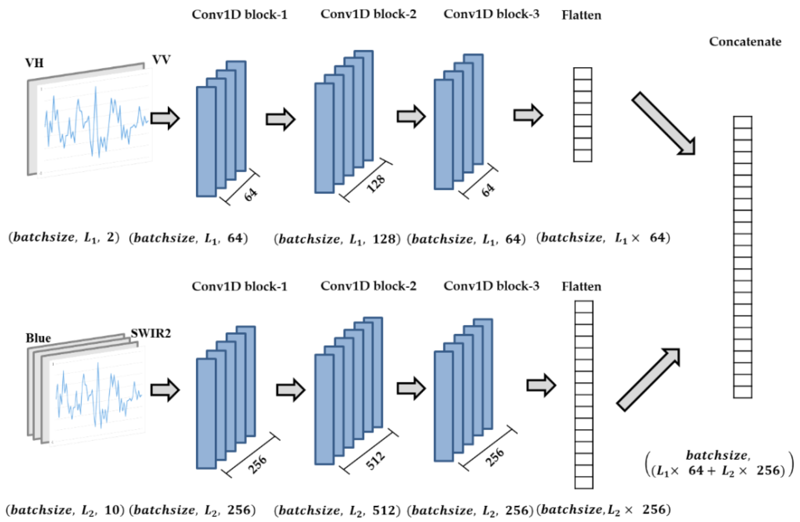
As noted, the sequence length of the S1A time series data with a 12-day interval was 14, and the sequence length of the S2 time series data with a 5-day interval was 35. The two types of time series data could not be input into a 1D CNN at the same time because their data acquisition dates were different. Therefore, the Dual-1DCNN model developed in this study integrated the time series data of S1A and S2 by building two 1D CNN modules: an S1A module and an S2 module (Figure 4).
Both the S1A module and S2 module had three Conv1D blocks and a flattened layer. A Conv1D block contains a Conv1D layer, a BN layer, and a ReLU layer. In the S1A module, the kernel sizes of the three Conv1D layers were 64, 128, and 64, and in the S2 module they were 256, 512, and 256. In each module, the kernel durations of the three Conv1D layers were set to 5, 4, and 3. The outputs of the S1A and S2 modules were concatenated by the concatenate layer and passed to a dropout layer (the dropout rate was set to 0.8) and an FC layer with 100 neurons. Finally, data were passed to a softmax classification layer with five neurons, which produced the predictive probabilities of all of the crop types in the input data.
As stated in Section 3.1, a sample can be expressed by , where , denotes the t-th observations of all variables, and represents the value of the d-th variable of . For all samples (1942), we first performed channel L2-norm (Equation (2)) before inputting them into the model. Note that the channel here is a band of S2 or a polarization of S1A in a data acquisition date, as follows:
Figure 5 shows the flow of data in each module. The input of the S1A module is a three-dimensional matrix with the shape of ; here, batchsize is the number of input samples in a batch, is the sequence length of the S1A time series with a 12-day interval, and 2 indicates the two polarizations (variables) of S1A. The input shape of the S2 module is ; here, is the sequence length of the S2 time series with a 5-day interval, and 10 indicates the ten spectrum bands (variables) of S2. Note that to find the best date for early crop-type classification, and are variables (see details in Section 3.4). In addition, the input was a pixel-wise image for the following reasons: (1) the main objective of this study was to investigate how early in the growing season the Dual-1DCNN could achieve optimal accuracy in crop-type classification by integrating S1A and S2 time series data; and (2) it was challenging to define the optimal size of spatial regions because the agriculture parcel was usually small in the study area—parcel segmentation is a direction for our future work.
The flattened layer converted the output of Conv1D block-3 in each module into a 1D single vector. Therefore, the output shape of the S1A module is , the output shape of the S2 module is , and the output of the concatenate layer is .
3.3. Evaluation
To make a comparative analysis, the Dual-1DCNN model was compared with two classical machine learning methods for crop-type mapping, including SVM and RF. The two metrics of overall accuracy (OA) and F1-score (F1) were adopted. OA was used to evaluate the performance of different models for crop-type classification, and F1 was used to evaluate the best date for the in-season detection of each crop type. The corresponding calculation formulas are as follows:
where TP, TN, FP, and FN denote numbers of pixels belonging to true positive, true negative, false positive, and false negative, respectively, in the confusion matrix.
3.4. Experimental Design
We called the DOY when S1A or S2 data were acquired in the growing season a “train date.” There was a total of 46 train dates excluding overlapping dates (Table 2). The first train date (DOY 103) was called the “start date”. From the start date to each train date, the number of times S1A or S2 data were obtained was the length of the corresponding sequence (i.e., L1 or L2, respectively). The time series of dates is shown in Table 2. Taking DOY 128 as an example, a total of 6 S2 images and 2 S1A images were acquired covering Hengshui City from 13 April to 9 May 2019.
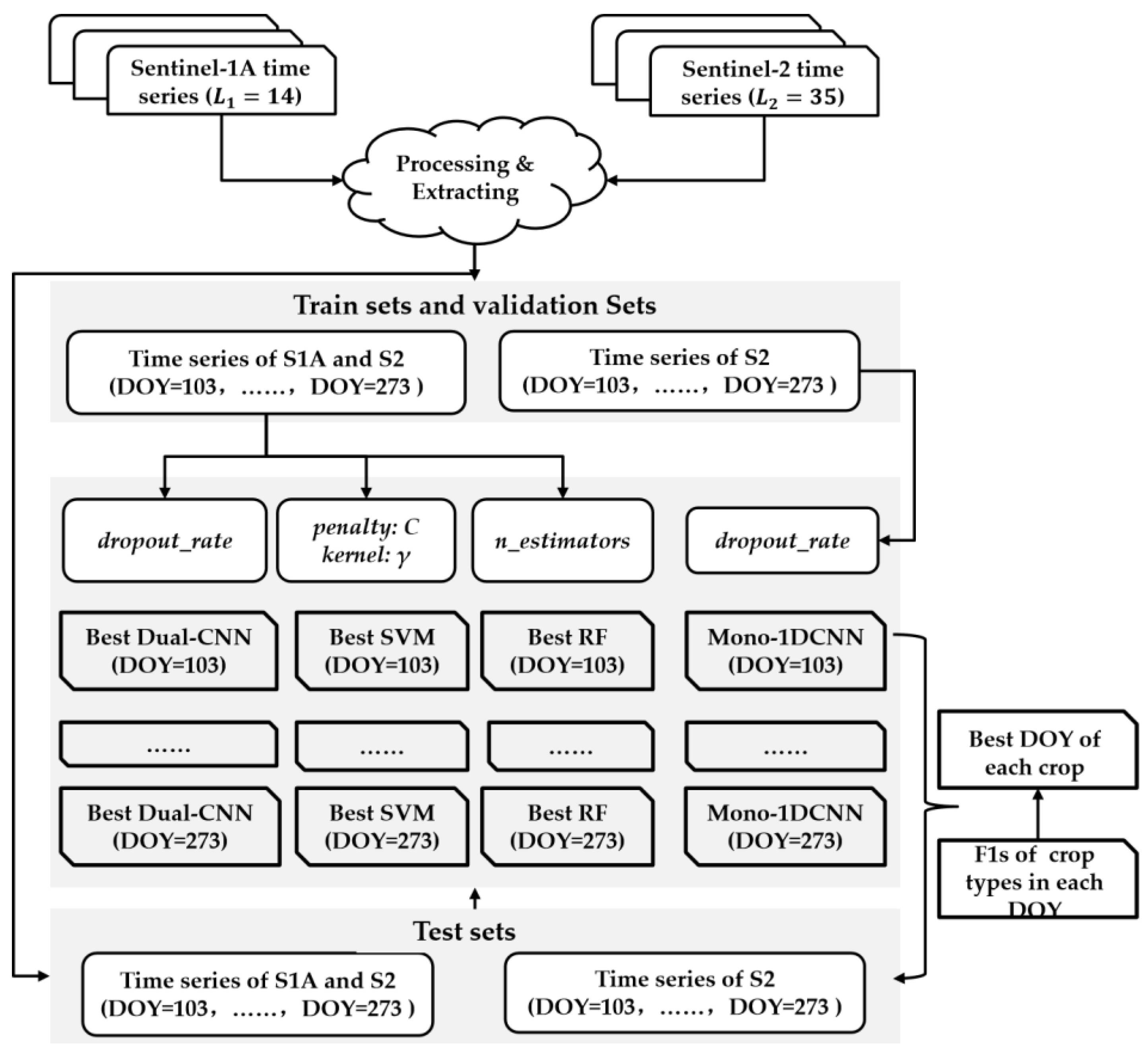
Figure 6 presents an overview of our experiments. We designed SVM, RF, and Mono-1DCNN as comparison models. Among them, the inputs of Dual-1DCNN, SVM, and RF were S1A and S2 data, and the input of Mono-1DCNN was S2 time series data. The input data included all of the S1A (VV, VH) and S2 (blue, green, red, RE1, RE2, RE3, NIR1, NIR2, SWIR1, SWIR2) data from the start date to the train date. First, we randomly selected 70% and 10% of samples of each crop type to form the training set and the validation set, respectively. The remaining samples (20%) constituted the test set because the distribution of the number of samples of the different crop types was uneven. Then, we conducted incremental training—that is, starting from the start date, the model was trained on each train date. The following training strategies were employed:
- (1)
- For the Dual-1DCNN model, the number of epochs was set to 10,000 with a batch size of 128 and an Adam optimizer [39]. We initially set the learning rate as and applied a global adaptation during each epoch. If the training cross-entropy error did not decrease for 100 epochs, we reduced it by 20% for the next epoch (the minimum learning rate was ). In addition, each training process was monitored through a callback function named ModelCheckpoint [40], and the model was saved when a better model of the training set was found. Apart from differences in input data, the training process of Mono-1DCNN was similar to that of the Dual-1DCNN.
- (2)
- For the SVM, we used the radial basis function (RBF)-based SVM (RBF-SVM), which requires two hyperparameters (i.e., penalty parameter C and kernel parameter ) to be tuned. During the optimization process, we selected from , and selected from .
- (3)
- The primary parameters of the RF model were the number of predictors at each decision tree node split (max_features) and the number of decision trees (n_estimators) to run. The features in this study were all channels of each input, and therefore, we set the parameter “max_features” with the default value (b is the number of channels) [41]. Additionally, the range of the grid search value for the “n_estimators” parameter varied from 100 to 10,000 with an interval of 100 [42].
To reduce the influence of random sample splitting bias, we performed five random splits to conduct five sets of training and five corresponding tests. This allowed us to compute the average performances of the five test sets. Finally, we evaluated the four types of models and attained the best date for each crop type for in-season mapping.
4. Results
4.1. Temporal Profiles of S1A and S2 Data
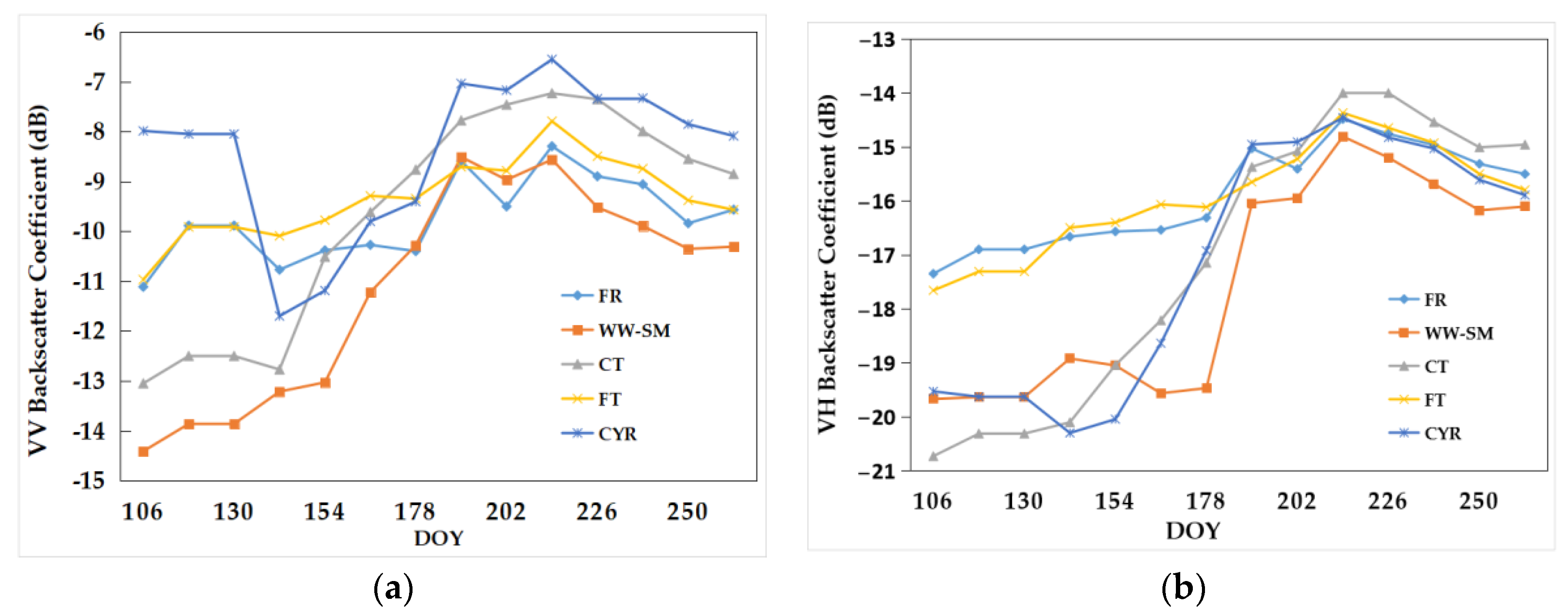
Figure 7 summarizes the temporal profiles of the VV and VH polarizations of the five crop types. We observed the following: (1) compared with VH curves, VV curves had less overlap or intersection, which was more conducive to the identification of the five crop types; (2) both VV and VH had the highest similarity for fruit tree and forest; and (3) for VH curves, common yam rhizome had a high similarity with winter wheat before DOY 130 (i.e., mid-May), whereas after DOY 190 (i.e., mid-July), it showed a similarity with fruit tree and forest.
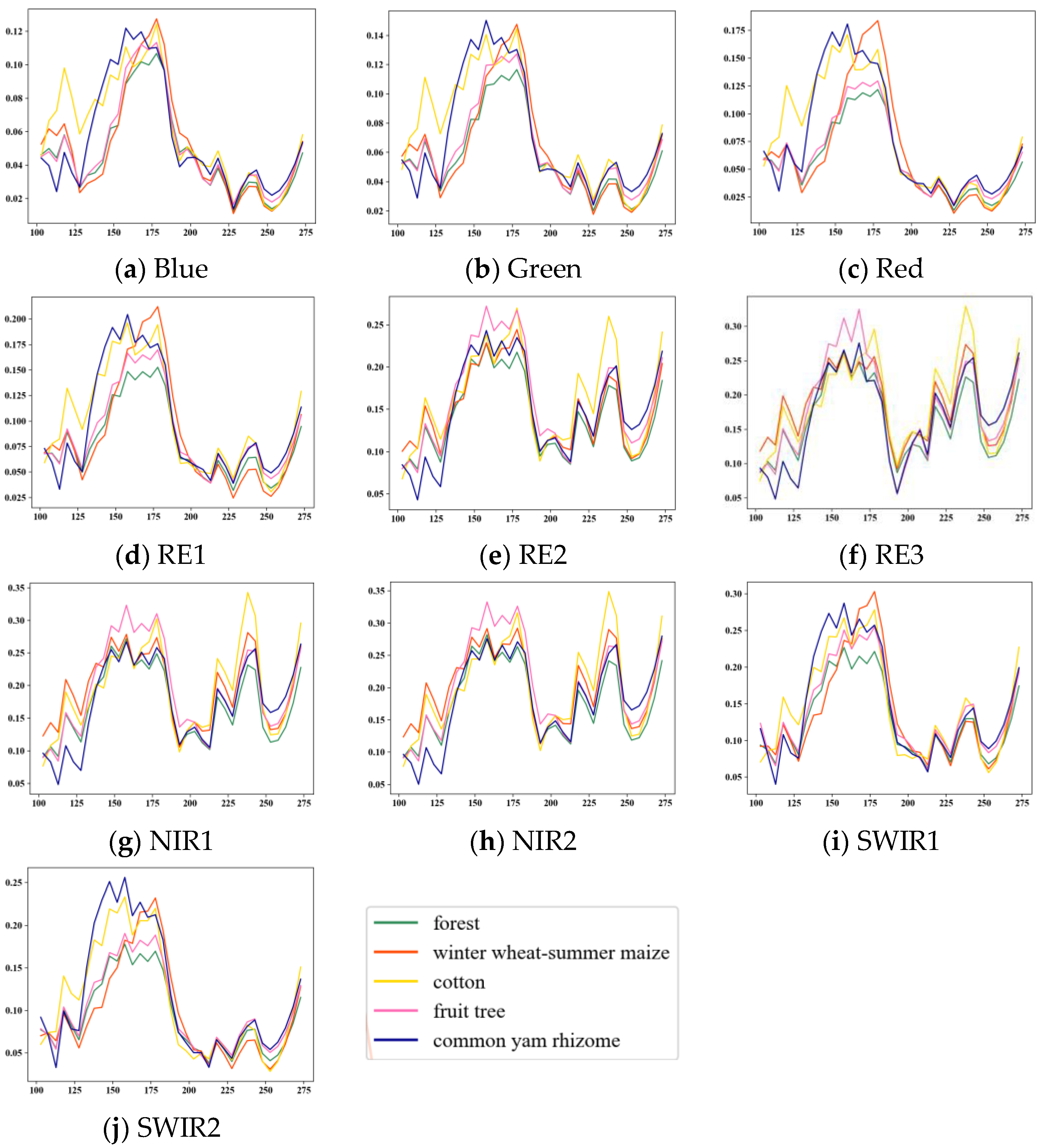
Figure 8 summarizes the temporal profiles of the ten spectrum bands of the five crop types. Each profile was obtained by time series linear interpolation and Savitzky–Golay smoothing illustrated the potential for gap-filling dense time series to contribute to crop-type classification.
As observed in the figure, the curves of different crop types from visible bands (Figure 8a–c) show obvious differences before DOY 183 (i.e., early July) and more intersections and overlaps after DOY 183, because all types were in the developing stage. The curves of RE1 were similar to the red spectrum curves, RE2 and RE3 were more similar to each other, and RE3 had the widest range of reflectivity. Furthermore, although the curves of NIR1 and NIR2 were very similar, those of SWIR1 and SWIR2 showed large differences, with the range of reflectivity of SWIR1 being larger.
Regarding different crop types, from DOY 103 to DOY 158, the visible and SWIR1/2 spectrum bands of cotton and common yam rhizome were significantly different from those of other crop types because they were in the growth phase. In addition, the RE2/3 and NIR1/2 spectrum bands of cotton were significantly enhanced during the period from DOY 218 to DOY 243 when cotton was maturing. The RE2/3 and NIR1/2 spectrum bands of fruit trees and forests showed a big difference from DOY 148 to DOY 178 but were very similar in other bands. Lastly, the visible, RE1, and SWIR1/2 spectrum bands of summer maize were significantly enhanced from DOY 163 to DOY 183, when summer maize was in the growth phase. In the same period, the curves of its other spectrum bands greatly overlapped with those of common yam rhizome.
4.2. Overall Assessment of Classification Accuracy
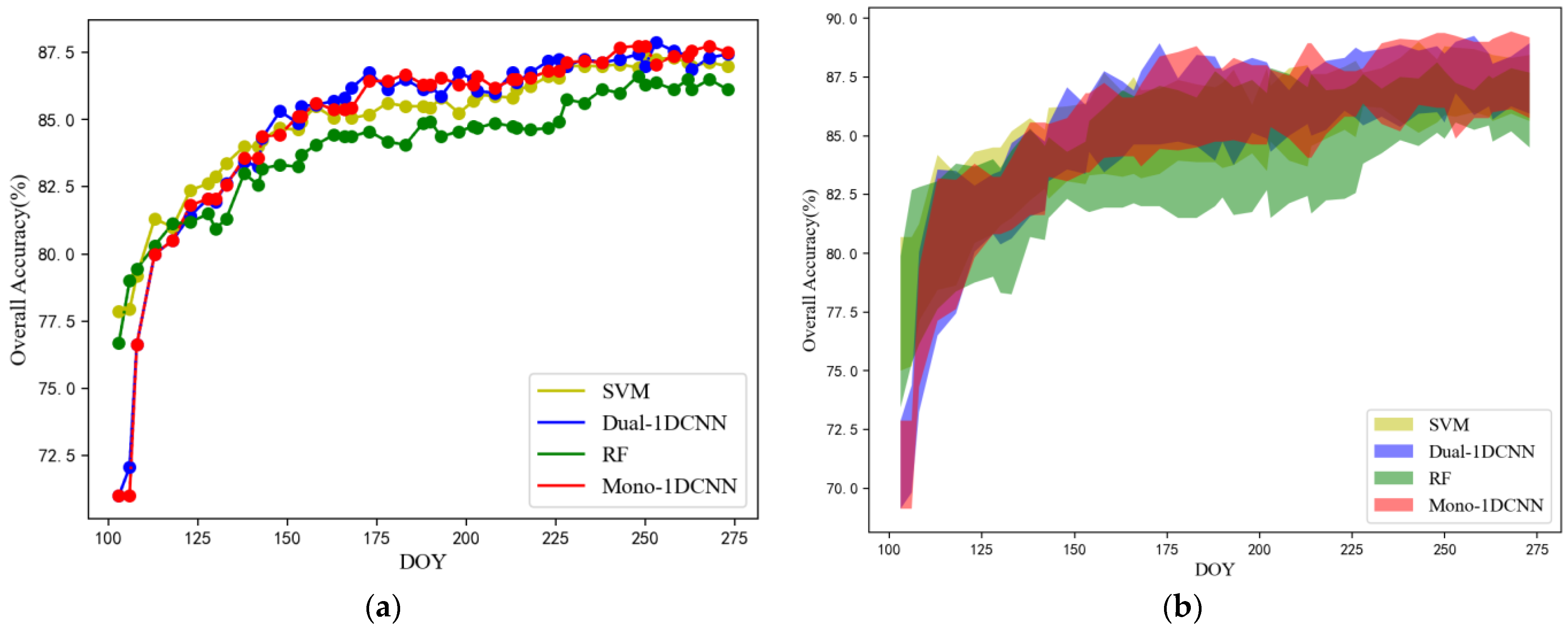
Figure 9 shows the evolution of the average classification accuracies of the five test sets as a function of the DOY time series in Table 2 using Dual-1DCNN (blue), SVM (yellow), RF (green), and Mono-1DCNN (red). The OA value given for each time point was the average from five repetitions, and the distance from the mean over five different random splits is shown in Figure 9b. Since the input of the Mono-1DCNN model was only S2 data, in order to keep the curve continuous, the accuracy of the model when S1A was acquired (such as DOY130 in Table 3) was the value of the previous time point (i.e., DOY128).
The curves of Dual-1DCNN and Mono-1DCNN were higher than that of SVM and RF overall, and Dual-1DCNN performed best. Specifically, the dates when the accuracy of Dual-1DCNN, Mono-1DCNN, SVM, and RF reached 85% for the first time were DOY 148, 153, 158, and 228, respectively. Considering that the summer maize growing season is DOY 166–259, the Dual-1DCNN achieved the highest accuracy of 86.77 (DOY 173) within one month since summer maize was sown. The above results prove that deep learning methods could extract deep classification features. At the same time, this was an important result supporting Dual-1DCNN as an effective method for crop-type identification by integrating S1A and S2 time series data. These results confirmed that Dual-1DCNN could provide more accurate and earlier results than SVM and RF.
4.3. Early Detection of Crop Types
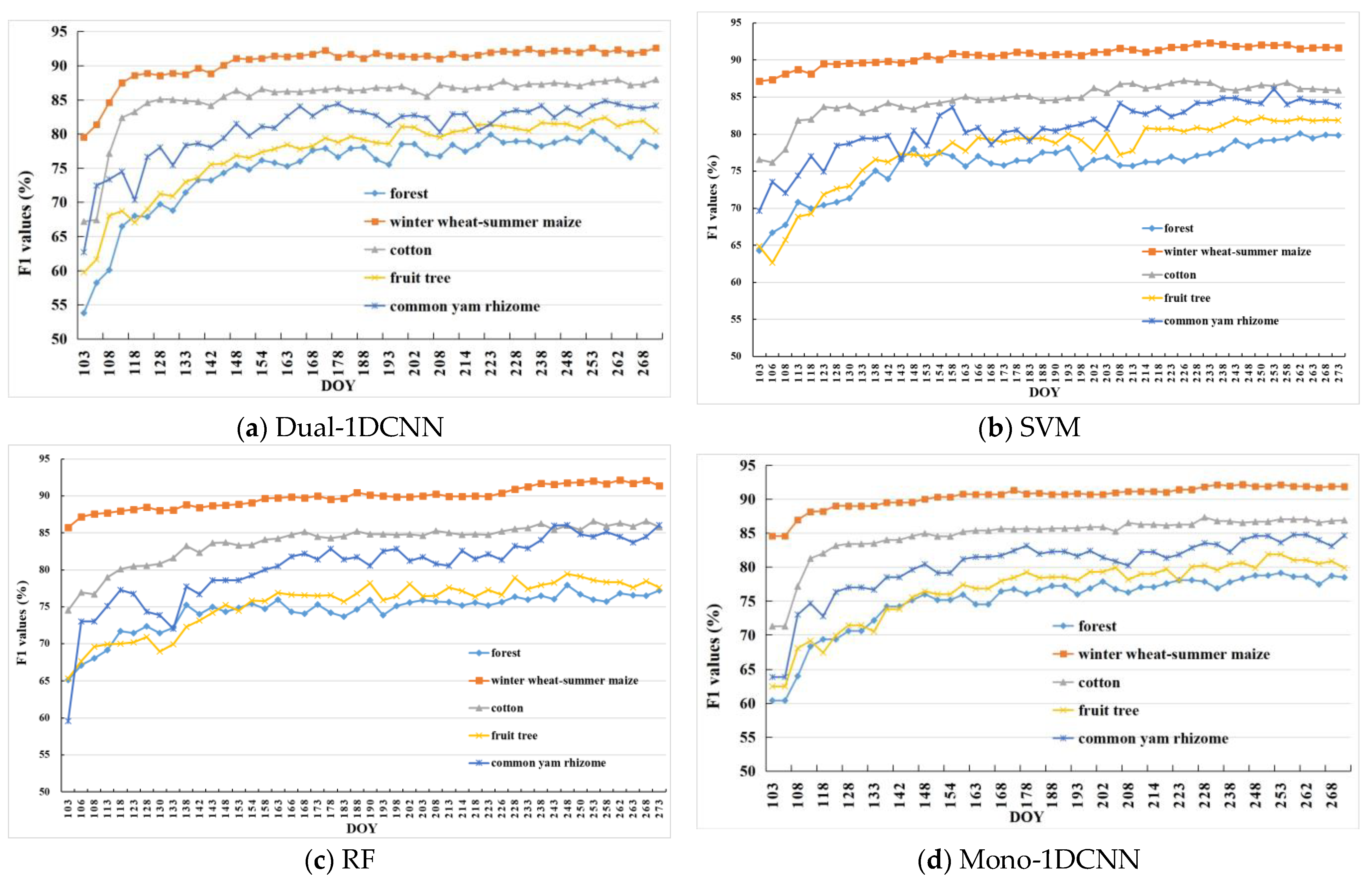
The best date for early mapping is usually different for each crop type. This work used F1 to evaluate the classification accuracy of different crop types. Figure 10 shows the F1 temporal profiles of each crop type by Dual-1DCNN, SVM, RF, and Mono-1DCNN. The F1 value given for each time point was the average over five different random splits.
First, for winter wheat and summer maize, all four methods achieved higher accuracy than for other crop types on each date. The Dual-1DCNN, SVM, RF, and Mono-1DCNN attained F1 values above 90% in the prophase stage, which was when wheat–summer maize had obvious phenological differences from other crop types. Second, as analyzed in Section 4.1, before DOY 158, cotton and common yam rhizome had obvious feature differences from other crop types; therefore, their F1 increased faster in the prophase stage with all four methods. Dual-1DCNN and Mono-1DCNN, however, extracted distinguishable features significantly better than the other two methods, especially on cotton. Third, all four methods performed unstably on common yam rhizome. As shown in Figure 8 and Figure 10b, the VH backscatter coefficients and reflectance values of common yam rhizome were similar more frequently than those of other crop types. This likely was due to the fact that the parcels of common yam rhizome usually were small, which resulted in more mixed-pixel samples. Finally, compared with other methods, curves obtained by Mono-1DCNN were relatively smoother, especially on common yam rhizome and forest, which was related to the missing DOY points (they were supplemented with F1s of their previous DOYs). In addition, it might also be related to the addition of S1A data for the other three models.
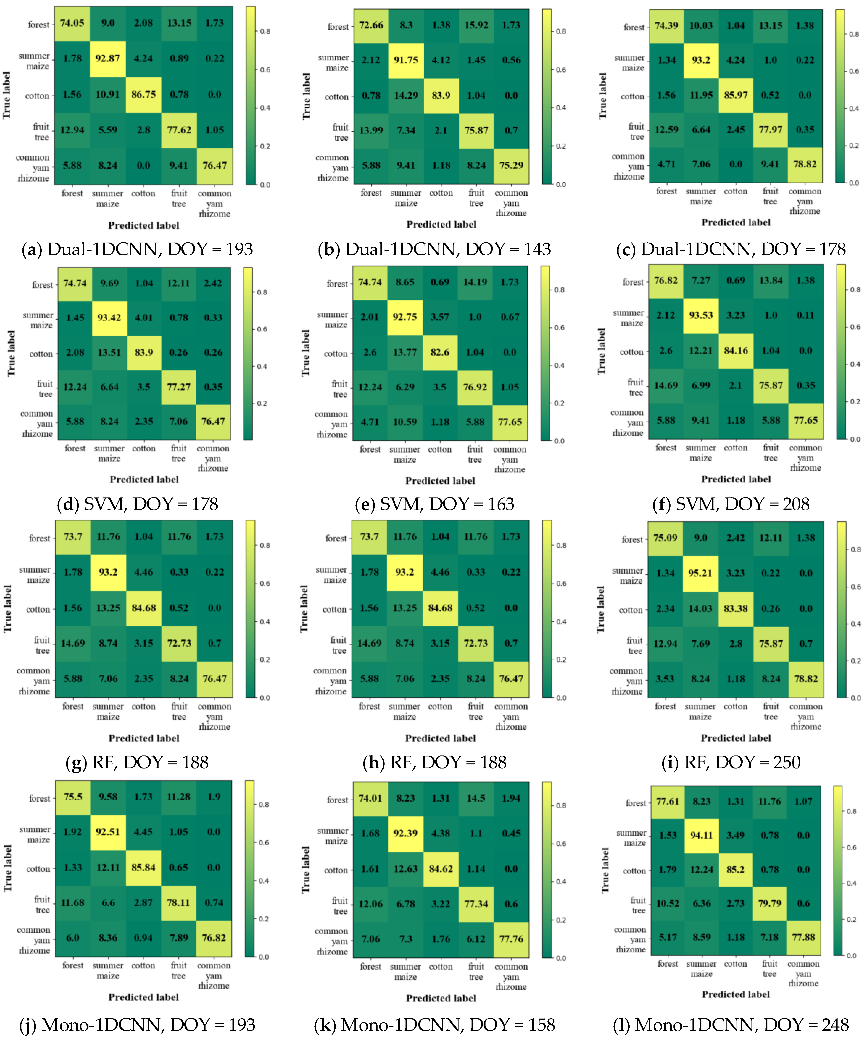
Considering the crop calendar, OA, and the F1 curves comprehensively, we used the following rules to determine the optimal in-season detection time: (1) for summer maize, it is the most widely distributed locally, and F1 was mostly greater than 90%, so the time when the maximum value of F1 was obtained within one month after sowing was taken; (2) for cotton, the highest accuracy of cotton was slightly higher than 85%, so the time when the accuracy reaches 85% for the first time was taken; (3) for common yam rhizome, the F1 values were almost all lower than 85%, and the time when it reached 84% for the first time was taken. According to the above rules, Table 4 summarizes the F1 for each crop type and the corresponding DOYs (i.e., in-season detection DOY) during the early season by Dual-1DCNN, SVM, and RF. Figure 11 shows the confusion matrices for the in-season detection DOYs. Overall, it was evident that Dual-1DCNN attained the highest F1 values on all four crop types. Furthermore, the in-season detection DOYs of cotton and common yam rhizome by Dual-1DCNN were all earlier than or the same as those obtained by SVM, RF, and Mono-1DCNN. These results confirmed that Dual-1DCNN was effective for the in-season detection of crop types.
5. Discussion
5.1. Performance of the Dual-1DCNN Algorithm
The earlier the crop type maps of the current growing season are obtained, the more beneficial it is for agricultural decision-making and management, especially when disasters occur as timely crop distribution information could support local governments in taking timely and rapid response measures. The results in Section 4 showed that all four types of models have achieved high accuracy (F1s were greater than 90%) on summer maize after sowing one month later. For the recognition time, the performance of traditional SVM and RF methods was comparable to that of deep learning methods, and the accuracies of the models based on S1A and S2 (Dual-1DCNN, SVM, and RF) were similar to the model (Mono-1DCNN) based on S2. This is mainly because Hengshui City is a winter wheat and summer maize rotation area, and the summer maize planting area was large and the samples were abundant. However, for cotton and common yam rhizome, which were not so numerous in sample size, Dual-1DCNN performed best, with its F1 reaching 85% within 2 months after cotton sowing, 15 days, 20 days, and 45 days ahead of Mono-1DCNN, SVM, and RF, respectively, and its extraction of common yam rhizome was achieved 1–2 months earlier than other methods within the acceptable accuracy. In addition, Dual-1DCNN achieved an overall accuracy of 85% at the earliest. Thus, Dual-1DCNN offered significant potential in the in-season detection of crop type. The literature [43] shows that compared with the single-sensor method, the combination of optical data and SAR data improves the overall accuracy by 6% to 10%. In the single-sensor method, optical data is better than SAR.
As described in Section 3.4, we conducted a wide range of value training on the hyperparameters of SVM and RF on each train date, that is to say, all results on each train date were the maximum values that SVM and RF could achieve in this study. The hyperparameters (including the architecture) of Dual-1DCNN were determined based on empirical parameters [11,24,44,45,46] and the hyperparameters on each train date were the same (except for the learning rate and dropout rate). We used these two methods to train the hyperparameters of the model because the DL algorithm required a lot of computing resources. In addition, to obtain an unbiased estimation of the generalization error in the Dual-1DCNN model, we conducted five-fold cross-validation [47]. When computing resources were met, our Dual-1DCNN model showed greater potential than SVM and RF.
Since the in-season detection of crop types required us to judge the best date for each crop type, we had to train the model many times, and the input time series data were different each time. Compared with the RNN series models, the 1D CNN model had fewer parameters, which enabled us to improve the training efficiency of the model. In addition, the input of the 1D CNN was a regular time series, that is, the time intervals of all features (i.e., spectrum or polarization) had to be the same. To address this requirement, we established the two-branch architecture, namely Dual-1DCNN in the application of S1A and S2 time series data. In addition, the Dual-1DCNN was not limited to the integration of S1A and S2. It is applicable to other different data sources, such as optical data sources (Landsat and S2) and SAR data sources (S1A and Gaofen-3). Therefore, this model can be extended to other regions, such as complex planting areas in southern China, which are characterized by frequent rainy weather, prolonged cloud cover, and rich crop types [48]. Optical remote sensing images in these areas are limited in data quality, and it is difficult to have enough images in the early crop period to support the in-season identification of different crop types. A dual-channel CNN model that synergistically utilizes optical and SAR data will greatly benefit the in-season identification of crops in these regions.
5.2. Limitations and Future Work
Although these results proved the effectiveness and advantages of the Dual-1DCNN algorithm for early detection of crop types by integrating S1A and S2 time series data, this study had some limitations that need to be overcome.
First, the classification accuracy was closely related to the crop types and the number of samples for each crop type [49,50]. The small sample numbers of cotton and common yam rhizome affected the classification accuracy. The planting area of summer maize in the entire study area, however, was much larger than that of cotton and common yam rhizome. We tried to reduce the number of training samples of summer maize, but the accuracy of the test samples would be reduced because of the complex relationship between geographical conditions and crops, and we required a uniform sample distribution. In future mapping work, we will conduct regional training of models for small areas of crops and build transferring models for large areas.
In addition, we analyzed the Dual-1DCNN algorithm on the pixel scale because our main objective was to investigate the use of new DL architecture for in-season detection of crop types by integrating S1A and S2 time series data. All of these results confirmed that our method performed better than the classical SVM and RF methods, and the effectiveness of deep extraction of S1A and S2 features using deep learning methods.
6. Conclusions
In-season crop type mapping is valuable for agricultural monitoring and management and holds great significance for global food security. In the context of the continuous growth of the global population, the use of remote-sensing data with high spatial and temporal resolutions to accurately, timely, and efficiently produce crop-type maps has become an important bottleneck in agricultural management. For smallholder agriculture in China, this task is even more challenging because of complex cropping patterns and a high degree of land fragmentation. To utilize more classification features and improve the timeliness of crop type detection, we described the Dual-1DCNN model. This algorithm offers two advantages: (1) It integrated and applied S1A and S2 time series data to detect crop types, which added phenological characteristics and spectral (or polarization) characteristics to the in-season data. (2) Compared with ML models, it explicitly considered the sequential relationship of multitemporal observations, which may be useful when dealing with time series inputs, and it was confirmed in Section 4. (3) Compared with the single-channel CNN method (Mono-1DCNN) that only used Sentinel-2 time series data, Dual-1DCNN improved the timeliness of in-season crop identification to a certain extent, especially for cotton and yam, whose sample sizes was small. In addition, this study focuses on addressing the potential of dense S1A and S2 time-series data integration to improve the temporal accuracy of early crop identification and provide base map information for agricultural monitoring as early as possible. In the future, we hope to improve the timeliness of crop mapping by tapping the potential of different data.
Author Contributions
Conceptualization and methodology, H.Z.; software, H.Z. and M.M.; validation, J.R. and G.T.; resources and data curation, H.Z. and M.M.; writing—original draft preparation, H.Z. and M.M.; writing—review and editing, J.R. and G.T.; funding acquisition, H.Z. and M.M. All authors have read and agreed to the published version of the manuscript.
Funding
This research was funded by Supported by National Key R&D Program of China and Shandong Province, China, grant number 2021YFB3901300; High resolution Earth observation System Project, grant number 09-H30G02-9001-20/22 and The Fundamental Research Funds for Central Non-profit Scientific Institution, grant number 1610132021021.
Conflicts of Interest
The authors declare no conflict of interest.
References
- Kolotii, A.; Kussul, N.; Shelestov, A.; Skakun, S.; Yailymov, B.; Basarab, R.; Lavreniuk, M.; Oliinyk, T.; Ostapenko, V. Comparison of biophysical and satellite predictors for wheat yield forecasting in Ukraine. Int. Arch. Photogramm. Remote Sens. Spatial Inf. Sci. 2015, XL-7/W3, 39–44. [Google Scholar] [CrossRef] [Green Version]
- Lobell, D.B.; David, T.; Christopher, S.; Eric, E.; Bertis, L. A scalable satellite-based crop yield mapper. Remote Sens. Environ. 2015, 164, 324–333. [Google Scholar] [CrossRef]
- Skakun, S.; Franch, B.; Vermote, E.; Roger, J.-C.; Becker-Reshef, I.; Justice, C.; Kussul, N. Early season large-area winter crop mapping using MODIS NDVI data, growing degree days information and a Gaussian mixture model. Remote Sens. Environ. 2017, 195, 244–258. [Google Scholar] [CrossRef]
- Homer, C.; Huang, C.; Yang, L.; Wylie, B.K.; Coan, M. Development of a 2001 national land-cover database for the United States. Photogramm. Eng. Remote Sens. 2004, 70, 829–840. [Google Scholar] [CrossRef] [Green Version]
- Khan, A.; Hansen, M.C.; Potapov, P.; Stehman, S.V.; Chatta, A.A. Landsat-based wheat mapping in the heterogeneous cropping system of Punjab, Pakistan. Int. J. Remote Sens. 2016, 37, 1391–1410. [Google Scholar] [CrossRef]
- Pôças, I.; Cunha, M.; Marcal, A.R.; Pereira, L.S. An evaluation of changes in a mountainous rural landscape of Northeast Portugal using remotely sensed data. Landsc. Urban Plan. 2011, 101, 253–261. [Google Scholar] [CrossRef] [Green Version]
- Skriver, H.; Mattia, F.; Satalino, G.; Balenzano, A.; Pauwels, V.R.; Verhoest, N.E.; Davidson, M. Crop classification using short-revisit multitemporal SAR data. IEEE J. Sel. Top. Appl. Earth Obs. Remote Sens. 2011, 4, 423–431. [Google Scholar] [CrossRef]
- Wardlow, B.D.; Egbert, S.L.; Kastens, J.H. Analysis of time-series MODIS 250 m vegetation index data for crop classification in the US Central Great Plains. Remote Sens. Environ. 2007, 108, 290–310. [Google Scholar] [CrossRef] [Green Version]
- Lebourgeois, V.; Dupuy, S.; Vintrou, É.; Ameline, M.; Butler, S.; Bégué, A. A combined random forest and OBIA classification scheme for mapping smallholder agriculture at different nomenclature levels using multisource data (simulated Sentinel-2 time series, VHRS and DEM). Remote Sens. 2017, 9, 259. [Google Scholar] [CrossRef] [Green Version]
- McCarty, J.; Neigh, C.; Carroll, M.; Wooten, M. Extracting smallholder cropped area in Tigray, Ethiopia with wall-to-wall sub-meter WorldView and moderate resolution Landsat 8 imagery. Remote Sens. Environ. 2017, 202, 142–151. [Google Scholar] [CrossRef]
- Zhao, H.; Chen, Z.; Jiang, H.; Jing, W.; Sun, L.; Feng, M. Evaluation of three deep learning models for early crop classification using sentinel-1A imagery time series—A case study in Zhanjiang, China. Remote Sens. 2019, 11, 2673. [Google Scholar] [CrossRef] [Green Version]
- Drusch, M.; Del Bello, U.; Carlier, S.; Colin, O.; Fernandez, V.; Gascon, F.; Hoersch, B.; Isola, C.; Laberinti, P.; Martimort, P. Sentinel-2: ESA’s optical high-resolution mission for GMES operational services. Remote Sens. Environ. 2012, 120, 25–36. [Google Scholar] [CrossRef]
- Dalla Mura, M.; Prasad, S.; Pacifici, F.; Gamba, P.; Chanussot, J.; Benediktsson, J.A. Challenges and opportunities of multimodality and data fusion in remote sensing. Proc. IEEE 2015, 103, 1585–1601. [Google Scholar] [CrossRef] [Green Version]
- McNairn, H.; Kross, A.; Lapen, D.; Caves, R.; Shang, J. Early season monitoring of corn and soybeans with TerraSAR-X and RADARSAT-2. Int. J. Appl. Earth Obs. Geoinf. 2014, 28, 252–259. [Google Scholar] [CrossRef]
- Cai, Y.; Guan, K.; Peng, J.; Wang, S.; Seifert, C.; Wardlow, B.; Li, Z. A high-performance and in-season classification system of field-level crop types using time-series Landsat data and a machine learning approach. Remote Sens. Environ. 2018, 210, 35–47. [Google Scholar] [CrossRef]
- Sonobe, R.; Yamaya, Y.; Tani, H.; Wang, X.; Kobayashi, N.; Mochizuki, K.-i. Crop classification from Sentinel-2-derived vegetation indices using ensemble learning. J. Appl. Remote Sens. 2018, 12, 026019. [Google Scholar] [CrossRef] [Green Version]
- Vreugdenhil, M.; Wagner, W.; Bauer-Marschallinger, B.; Pfeil, I.; Teubner, I.; Rüdiger, C.; Strauss, P. Sensitivity of Sentinel-1 backscatter to vegetation dynamics: An Austrian case study. Remote Sens. 2018, 10, 1396. [Google Scholar] [CrossRef] [Green Version]
- Ndikumana, E.; Ho Tong Minh, D.; Baghdadi, N.; Courault, D.; Hossard, L. Deep recurrent neural network for agricultural classification using multitemporal SAR Sentinel-1 for Camargue, France. Remote Sens. 2018, 10, 1217. [Google Scholar] [CrossRef] [Green Version]
- Zhong, L.; Hu, L.; Zhou, H. Deep learning based multi-temporal crop classification. Remote Sens. Environ. 2019, 221, 430–443. [Google Scholar] [CrossRef]
- Saha, S.; Mou, L.; Qiu, C.; Zhu, X.X.; Bovolo, F.; Bruzzone, L. Unsupervised deep joint segmentation of multitemporal high-resolution images. IEEE Trans. Geosci. Remote Sens. 2020, 58, 8780–8792. [Google Scholar] [CrossRef]
- Yuan, Q.; Shen, H.; Li, T.; Li, Z.; Li, S.; Jiang, Y.; Xu, H.; Tan, W.; Yang, Q.; Wang, J. Deep learning in environmental remote sensing: Achievements and challenges. Remote Sens. Environ. 2020, 241, 111716. [Google Scholar] [CrossRef]
- Zhang, F.; Yao, X.; Tang, H.; Yin, Q.; Hu, Y.; Lei, B. Multiple mode SAR raw data simulation and parallel acceleration for Gaofen-3 mission. IEEE J. Sel. Top. Appl. Earth Obs. Remote Sens. 2018, 11, 2115–2126. [Google Scholar] [CrossRef]
- Ismail Fawaz, H.; Forestier, G.; Weber, J.; Idoumghar, L.; Muller, P.-A. Deep learning for time series classification: A review. Data Min. Knowl. Discov. 2019, 33, 917–963. [Google Scholar] [CrossRef] [Green Version]
- Zheng, Y.; Liu, Q.; Chen, E.; Ge, Y.; Zhao, J.L. Time series classification using multi-channels deep convolutional neural networks. In Proceedings of the Web-Age Information Management: 15th International Conference, WAIM 2014, Macau, China, 16–18 June 2014; pp. 298–310. [Google Scholar]
- Cho, K.; Van Merriënboer, B.; Bahdanau, D.; Bengio, Y. On the properties of neural machine translation: Encoder-decoder approaches. arXiv 2014, arXiv:1409.1259. [Google Scholar]
- Liao, C.; Wang, J.; Xie, Q.; Baz, A.A.; Huang, X.; Shang, J.; He, Y. Synergistic use of multi-temporal RADARSAT-2 and VENµS data for crop classification based on 1D convolutional neural network. Remote Sens. 2020, 12, 832. [Google Scholar] [CrossRef] [Green Version]
- Zhao, W.; Qu, Y.; Chen, J.; Yuan, Z. Deeply synergistic optical and SAR time series for crop dynamic monitoring. Remote Sens. Environ. 2020, 247, 111952. [Google Scholar] [CrossRef]
- Ienco, D.; Interdonato, R.; Gaetano, R.; Minh, D.H.T. Combining Sentinel-1 and Sentinel-2 Satellite Image Time Series for land cover mapping via a multi-source deep learning architecture. ISPRS J. Photogramm. Remote Sens. 2019, 158, 11–22. [Google Scholar] [CrossRef]
- Sak, H.; Senior, A.; Beaufays, F. Long short-term memory recurrent neural network architectures for large scale acoustic modeling. In Proceedings of the Fifteenth Annual Conference of the International Speech Communication Association, Singapore, 14–18 September 2014. [Google Scholar]
- Sophie, B.; Arias, M.; Cara, C.; Dedieu, G.; Guzzonato, E.; Hagolle, O.; Inglada, J.; Matton, N.; Morin, D.; Popescu, R. Building a data set over 12 globally distributed sites to support the development of agriculture monitoring applications with sentinel-2. Remote Sens. 2015, 7, 16062–16090. [Google Scholar]
- Qiu, S.; Zhu, Z.; He, B. Fmask 4.0: Improved cloud and cloud shadow detection in Landsats 4–8 and Sentinel-2 imagery. Remote Sens. Environ. 2019, 231, 111205. [Google Scholar] [CrossRef]
- Kandasamy, S.; Baret, F.; Verger, A.; Neveux, P.; Weiss, M. A comparison of methods for smoothing and gap filling time series of remote sensing observations: Application to MODIS LAI products. Biogeosciences 2012, 10, 4055–4071. [Google Scholar] [CrossRef] [Green Version]
- Chen, J.; Jönsson, P.; Tamura, M.; Gu, Z.; Matsushita, B.; Eklundh, L. A simple method for reconstructing a high-quality NDVI time-series data set based on the Savitzky–Golay filter. Remote Sens. Environ. 2004, 91, 332–344. [Google Scholar] [CrossRef]
- LeCun, Y.; Bengio, Y.; Hinton, G. Deep learning. Nature 2015, 521, 436–444. [Google Scholar] [CrossRef] [PubMed]
- Krizhevsky, A.; Sutskever, I.; Hinton, G.E. Imagenet classification with deep convolutional neural networks. Commun. ACM 2017, 60, 84–90. [Google Scholar] [CrossRef] [Green Version]
- Zeiler, M.D.; Fergus, R. Stochastic pooling for regularization of deep convolutional neural networks. arXiv 2013, arXiv:1301.3557. [Google Scholar]
- Ioffe, S.; Szegedy, C. Batch normalization: Accelerating deep network training by reducing internal covariate shift. In Proceedings of the International Conference on Machine Learning, Lille, France, 6–11 July 2015; pp. 448–456. [Google Scholar]
- Hu, W.; Huang, Y.; Wei, L.; Zhang, F.; Li, H. Deep convolutional neural networks for hyperspectral image classification. J. Sens. 2015, 2015, 258619. [Google Scholar] [CrossRef] [Green Version]
- Kingma, D.P.; Ba, J. Adam: A method for stochastic optimization. arXiv 2014, arXiv:1412.6980. [Google Scholar]
- Lu, L.; Meng, X.; Mao, Z.; Karniadakis, G.E. DeepXDE: A deep learning library for solving differential equations. SIAM Rev. 2021, 63, 208–228. [Google Scholar] [CrossRef]
- Goldstein, B.A.; Polley, E.C.; Briggs, F.B. Random forests for genetic association studies. Stat. Appl. Genet. Mol. Biol. 2011, 10, 32. [Google Scholar] [CrossRef]
- Probst, P.; Wright, M.; Boulesteix, A. Hyperparameters and tuning strategies for random forest. WIREs Data Min. Knowl. Discov. 2019, 9, e1301. [Google Scholar] [CrossRef] [Green Version]
- Blickensdörfer, L.; Schwieder, M.; Pflugmacher, D.; Nendel, C.; Erasmi, S.; Hostert, P. Mapping of crop types and crop sequences with combined time series of Sentinel-1, Sentinel-2 and Landsat 8 data for Germany. Remote Sens. Environ. 2022, 269, 112831. [Google Scholar] [CrossRef]
- Hatami, N.; Gavet, Y.; Debayle, J. Classification of time-series images using deep convolutional neural networks. In Proceedings of the Tenth International Conference on Machine Vision (ICMV 2017), Vienna, Austria, 13–15 November 2017; pp. 242–249. [Google Scholar]
- Srivastava, N.; Hinton, G.; Krizhevsky, A.; Sutskever, I.; Salakhutdinov, R. Dropout: A simple way to prevent neural networks from overfitting. J. Mach. Learn. Res. 2014, 15, 1929–1958. [Google Scholar]
- Wang, H.; Wang, Y.; Zhang, Q.; Xiang, S.; Pan, C. Gated convolutional neural network for semantic segmentation in high-resolution images. Remote Sens. 2017, 9, 446. [Google Scholar] [CrossRef] [Green Version]
- Kohavi, R. A study of cross-validation and bootstrap for accuracy estimation and model selection. In Proceedings of the International Joint Conference on Artificial Intelligence, Montreal, QB, Canada, 20–25 August 1995; pp. 1137–1145. [Google Scholar]
- Xie, L.; Zhang, H.; Li, H.; Wang, C. A unified framework for crop classification in southern China using fully polarimetric, dual polarimetric, and compact polarimetric SAR data. Int. J. Remote Sens. 2015, 36, 3798–3818. [Google Scholar] [CrossRef]
- Douzas, G.; Bacao, F.; Fonseca, J.; Khudinyan, M. Imbalanced Learning in Land Cover Classification: Improving Minority Classes’ Prediction Accuracy Using the Geometric SMOTE Algorithm. Remote Sens. 2019, 11, 3040. [Google Scholar] [CrossRef] [Green Version]
- Sun, F.; Fang, F.; Wang, R.; Wan, B.; Guo, Q.; Li, H.; Wu, X. An Impartial Semi-Supervised Learning Strategy for Imbalanced Classification on VHR Images. Sensors 2020, 20, 6699. [Google Scholar] [CrossRef]
Figure 1.
The study area and sample distribution: (a) Hebei Province, the green area is Hengshui City; (b) Samples in Hengshui City.
Figure 1.
The study area and sample distribution: (a) Hebei Province, the green area is Hengshui City; (b) Samples in Hengshui City.

Figure 2.
Crop calendar of winter wheat-summer maize, cotton, and common yam rhizome in Hengshui, China. DOY, day of year.
Figure 2.
Crop calendar of winter wheat-summer maize, cotton, and common yam rhizome in Hengshui, China. DOY, day of year.

Figure 3.
The main investigated types in July.

Figure 4.
The Dual-1DCNN model.

Figure 5.
Flow of S1A time series data and S2 time series data.

Figure 6.
Overview of experiments. L1: the length of S1A time series imagery; L2: the length of S2 time series imagery.
Figure 6.
Overview of experiments. L1: the length of S1A time series imagery; L2: the length of S2 time series imagery.

Figure 7.
Temporal profiles of the five crop types with respect to (a) VV and (b) VH backscatter coefficients (dB).
Figure 7.
Temporal profiles of the five crop types with respect to (a) VV and (b) VH backscatter coefficients (dB).

Figure 8.
Time series profiles. RE, red edge; NIR, near-infrared; SWIR1, shortwave infrared.

Figure 9.
OA profiles of the four methods, (a) the mean values over five different random splits (b) the distance from the mean over five different random splits.
Figure 9.
OA profiles of the four methods, (a) the mean values over five different random splits (b) the distance from the mean over five different random splits.

Figure 10.
F1 values of each crop type at every train date (the average over five different random splits).
Figure 10.
F1 values of each crop type at every train date (the average over five different random splits).

Figure 11.
Confusion matrices for in-season detection DOYs of summer maize, cotton, and common yam rhizome. Values in matrices indicate the percentage of points available in the “true label” and are the average of five test sets.
Figure 11.
Confusion matrices for in-season detection DOYs of summer maize, cotton, and common yam rhizome. Values in matrices indicate the percentage of points available in the “true label” and are the average of five test sets.


Table 1.
Number of samples per type.
| Class Label | 1 | 2 | 3 | 4 | 5 | Total |
|---|---|---|---|---|---|---|
| Class type | forest | summer maize | cotton | fruit tree | common yam rhizome | |
| Number | 289 | 897 | 385 | 286 | 85 | 1942 |
Table 2.
Time series of dates when we acquired S1A or S2 data. DOY: day of year in 2019; L1: the length of S1A time series imagery; L2: the length of S2 time series imagery.
Table 2.
Time series of dates when we acquired S1A or S2 data. DOY: day of year in 2019; L1: the length of S1A time series imagery; L2: the length of S2 time series imagery.
| DOY | 103 | 106 | 108 | 113 | 118 | 123 | 128 | 130 | 133 | 138 | 142 | 143 | 148 | 153 | 154 | 158 |
| L1 | 0 | 1 | 1 | 1 | 2 | 2 | 2 | 3 | 3 | 3 | 4 | 4 | 4 | 4 | 5 | 5 |
| L2 | 1 | 1 | 2 | 3 | 4 | 5 | 6 | 6 | 7 | 8 | 8 | 9 | 10 | 11 | 11 | 12 |
| DOY | 163 | 166 | 168 | 173 | 178 | 183 | 188 | 190 | 193 | 198 | 202 | 203 | 208 | 213 | 214 | 218 |
| L1 | 5 | 6 | 6 | 6 | 7 | 7 | 7 | 8 | 8 | 8 | 9 | 9 | 9 | 9 | 10 | 10 |
| L2 | 13 | 13 | 14 | 15 | 16 | 17 | 18 | 18 | 19 | 20 | 20 | 21 | 22 | 23 | 23 | 24 |
| DOY | 223 | 226 | 228 | 233 | 238 | 243 | 248 | 250 | 253 | 258 | 262 | 263 | 268 | 273 | ||
| L1 | 10 | 11 | 11 | 11 | 12 | 12 | 12 | 13 | 13 | 13 | 14 | 14 | 14 | 14 | ||
| L2 | 25 | 25 | 26 | 27 | 28 | 29 | 30 | 30 | 31 | 32 | 32 | 33 | 34 | 35 |
Table 3.
OA and standard deviation at every train date. OA, average over five different random splits; CNN, convolutional neural network; SVM, support vector machine; RF, random forest; DOY, day of year; “/” indicates that there was no new S2 data acquisition for that day.
Table 3.
OA and standard deviation at every train date. OA, average over five different random splits; CNN, convolutional neural network; SVM, support vector machine; RF, random forest; DOY, day of year; “/” indicates that there was no new S2 data acquisition for that day.
| DOY | 103 | 106 | 108 | 113 | 118 | 123 | 128 | 130 |
| Dual-1DCNN | 71.00 ± 1.90 | 72.09 ± 2.3 | 76.63 ± 3.41 | 80.02 ± 3.53 | 80.49 ± 3.03 | 81.46 ± 1.41 | 82.08 ± 1.27 | 81.93 ± 1.56 |
| SVM | 77.86 ± 2.83 | 77.96 ± 2.75 | 79.2 ± 2.05 | 81.31 ± 2.85 | 81.00 ± 2.39 | 82.39 ± 1.94 | 82.65 ± 1.84 | 82.85 ± 1.65 |
| RF | 76.67 ± 3.21 | 78.99 ± 3.68 | 79.46 ± 3.35 | 80.33 ± 2.72 | 81.1 ± 2.72 | 81.21 ± 2.46 | 81.51 ± 2.48 | 80.95 ± 2.65 |
| Mono-1DCNN | 71 ± 1.90 | / | 76.85 ± 2.53 | 80.15 ± 3.01 | 80.36 ± 2.74 | 81.82 ± 2.01 | 82.05 ± 1.21 | / |
| DOY | 133 | 138 | 142 | 143 | 148 | 153 | 154 | 158 |
| Dual-1DCNN | 82.65 ± 2.03 | 83.42 ± 1.83 | 83.27 ± 1.48 | 84.30 ± 1.23 | 85.32 ± 1.77 | 84.86 ± 1.46 | 85.53 ± 1.19 | 85.58 ± 2.14 |
| SVM | 83.37 ± 1.84 | 83.99 ± 1.75 | 83.99 ± 1.24 | 84.24 ± 1.95 | 84.66 ± 1.58 | 84.65 ± 1.72 | 84.91 ± 1.57 | 85.53 ± 2.15 |
| RF | 81.31 ± 3.04 | 83.01 ± 2.31 | 82.55 ± 2.00 | 83.21 ± 1.74 | 83.32 ± 1.02 | 83.27 ± 1.48 | 83.68 ± 1.92 | 84.04 ± 2.13 |
| Mono-1DCNN | 82.54 ± 1.52 | 83.59 ± 1.95 | / | 84.36 ± 1.14 | 84.41 ± 1.32 | 85.13 ± 1.69 | / | 85.64 ± 1.58 |
| DOY | 163 | 166 | 168 | 173 | 178 | 183 | 188 | 190 |
| Dual-1DCNN | 85.69 ± 1.63 | 85.79 ± 1.15 | 86.20 ± 1.55 | 86.77 ± 2.15 | 86.10 ± 1.34 | 86.51 ± 1.95 | 86.15 ± 2.20 | 86.25 ± 1.49 |
| SVM | 85.07 ± 1.80 | 85.43 ± 2.07 | 85.06 ± 1.87 | 85.17 ± 1.82 | 85.63 ± 1.72 | 85.53 ± 1.64 | 85.48 ± 1.61 | 85.43 ± 1.82 |
| RF | 84.45 ± 2.50 | 84.40 ± 2.26 | 84.40 ± 2.38 | 84.55 ± 2.58 | 84.19 ± 2.72 | 84.04 ± 2.56 | 84.86 ± 2.87 | 84.92 ± 2.56 |
| Mono-1DCNN | 85.38 ± 1.26 | / | 85.44 ± 1.75 | 86.41 ± 1.95 | 86.46 ± 2.08 | 86.67 ± 2.14 | 86.31 ± 1.56 | / |
| DOY | 193 | 198 | 202 | 203 | 208 | 213 | 214 | 218 |
| Dual-1DCNN | 85.89 ± 2.13 | 86.72 ± 1.59 | 86.51 ± 1.64 | 86.05 ± 1.75 | 85.99 ± 0.97 | 86.72 ± 1.23 | 86.36 ± 1.39 | 86.72 ± 1.48 |
| SVM | 85.79 ± 2.02 | 85.27 ± 1.03 | 85.69 ± 2.19 | 85.94 ± 1.19 | 85.89 ± 1.96 | 85.84 ± 2.15 | 86.10 ± 1.54 | 86.25 ± 1.39 |
| RF | 84.35 ± 2.74 | 84.55 ± 2.81 | 84.76 ± 2.06 | 84.66 ± 3.19 | 84.86 ± 2.75 | 84.76 ± 2.30 | 84.66 ± 2.95 | 84.60 ± 2.36 |
| Mono-1DCNN | 86.56 ± 1.73 | 86.3 ± 1.69 | / | 86.61 ± 1.22 | 86.2 ± 1.35 | 86.51 ± 2.42 | / | 86.58 ± 1.54 |
| DOY | 223 | 226 | 228 | |||||
| Dual-1DCNN | 87.18 ± 1.14 | 87.23 ± 1.50 | 87.02 ± 1.56 | |||||
| SVM | 86.61 ± 1.34 | 86.56 ± 1.63 | 86.97 ± 0.69 | |||||
| RF | 84.66 ± 2.36 | 84.91 ± 2.34 | 85.74 ± 1.90 | |||||
| Mono-1DCNN | 86.79 ± 0.96 | / | 87.12 ± 0.77 |
Table 4.
F1 value of each crop type at every train date (the average over five different random splits). CNN, convolutional neural network; SVM, support vector machine; RF, random forest; DOY, day of year.
Table 4.
F1 value of each crop type at every train date (the average over five different random splits). CNN, convolutional neural network; SVM, support vector machine; RF, random forest; DOY, day of year.
| Methods | Indices | Summer Maize | Cotton | Common Yam Rhizome |
|---|---|---|---|---|
| Dual-1DCNN | In-season detection DOY | 193 | 143 | 178 |
| F1 value | 91.48 | 85.45 | 84.38 | |
| SVM | In-season detection DOY | 178 | 163 | 208 |
| F1 value | 91.04 | 85.04 | 84.18 | |
| RF | In-season detection DOY | 188 | 188 | 250 |
| F1 value | 90.44 | 85.24 | 84.8 | |
| Mono-1DCNN | In-season detection DOY | 193 | 158 | 248 |
| F1 value | 90.84 | 85.2 | 84.6 |
Disclaimer/Publisher’s Note: The statements, opinions and data contained in all publications are solely those of the individual author(s) and contributor(s) and not of MDPI and/or the editor(s). MDPI and/or the editor(s) disclaim responsibility for any injury to people or property resulting from any ideas, methods, instructions or products referred to in the content. |
© 2023 by the authors. Licensee MDPI, Basel, Switzerland. This article is an open access article distributed under the terms and conditions of the Creative Commons Attribution (CC BY) license (https://creativecommons.org/licenses/by/4.0/).
Share and Cite
MDPI and ACS Style
Mao, M.; Zhao, H.; Tang, G.; Ren, J. In-Season Crop Type Detection by Combing Sentinel-1A and Sentinel-2 Imagery Based on the CNN Model. Agronomy 2023, 13, 1723. https://doi.org/10.3390/agronomy13071723
AMA Style
Mao M, Zhao H, Tang G, Ren J. In-Season Crop Type Detection by Combing Sentinel-1A and Sentinel-2 Imagery Based on the CNN Model. Agronomy. 2023; 13(7):1723. https://doi.org/10.3390/agronomy13071723
Chicago/Turabian StyleMao, Mingxiang, Hongwei Zhao, Gula Tang, and Jianqiang Ren. 2023. "In-Season Crop Type Detection by Combing Sentinel-1A and Sentinel-2 Imagery Based on the CNN Model" Agronomy 13, no. 7: 1723. https://doi.org/10.3390/agronomy13071723
Note that from the first issue of 2016, this journal uses article numbers instead of page numbers. See further details here.