Article

Multi-Scale Correlation between Soil Loss and Natural Rainfall on Sloping Farmland Using the Hilbert–Huang Transform in Southwestern China

1
College of Forestry, Sichuan Agricultural University, Chengdu 611130, China
2
College of Resources Science, Sichuan Agricultural University, Chengdu 611130, China
3
College of Water Resources and Hydropower Engineering, Sichuan Agricultural University, Yaan 625014, China
*
Author to whom correspondence should be addressed.
Agronomy 2023, 13(6), 1492; https://doi.org/10.3390/agronomy13061492
Submission received: 19 March 2023 / Revised: 12 May 2023 / Accepted: 19 May 2023 / Published: 29 May 2023
(This article belongs to the Section Farming Sustainability)

Abstract

:
The Hilbert–Huang transform (HHT) has been used as a powerful tool for analyzing nonlinear and nonstationary time series. Soil loss is controlled by complicated physical processes and thus fluctuates with nonlinearity and nonstationarity over time. In order to further clarify the relationship between rainfall, surface runoff, and sediment yield, this study adopted the HHT to analyze these characteristics through multiple time scales and investigated their relationship through time-dependent intrinsic correlation (TDIC) in the time series. A six-year study (2015–2020) was conducted on sloping farmlands to explore the relationships between soil loss and rainfall in southwest China. Time series of soil loss and rainfall were identified as the relevant characteristics at different time scales based on the method of HHT. Local correlation between the soil loss and runoff was carried out by the method of TDIC. The original time series of the rainfall, runoff, and soil loss were decomposed into eight intrinsic mode functions (IMFs) and a residue by ensemble empirical mode decomposition (EEMD). The residue indicated that the rainfall and runoff increased and then decreased during the maize-growing season from 2015 to 2020, whereas the soil loss gradually decreased. IMF1 and IMF2 accounted for nearly 80% of the temporal variations in rainfall, runoff, and soil loss, indicating that the variables varied the most at short time scales. The TDIC analysis showed that strong and positive correlations between the soil loss, rainfall, and runoff prevailed over the entire time domain at the scales of IMF1 and IMF2, indicating the rapid response of the soil loss to rainfall and runoff at short time scales. Time-varying correlations were observed at the IMF3–IMF5 scales. At the IMF7 scale, an evident switchover in the nature of the correlation was identified during the years 2018 and 2019; this could be related to a sudden rainstorm under low vegetation coverage conditions. The EEMD-based TDIC tool is an effective means to clarify the relationship between soil loss, rainfall, and runoff. Our results provide a better understanding of the relationship between soil loss and rainfall varied with time at multiple time scales. Short-term heavy rainfall and rapid surface runoff are the important factors causing serious soil and water loss on a short time scale in a mountainous region with yellow soil, which is of great significance for the construction of a regional soil erosion prediction model.

1. Introduction

Soil loss can cause land degradation, grain reduction, eutrophication, etc., and has become a major threat to agricultural ecosystem sustainability [1,2,3]. Sloping farmlands are believed to be the main sources of soil loss in watersheds, particularly in the hilly areas of China [4]. This has led to great concern regarding the fluctuation of soil loss under long-term agricultural management [5]. However, soil loss is controlled by different physical processes, each with a specific time scale of variability, and fluctuates at multiple time scales [6,7,8,9]. The fact that, in nature, the effects of different processes at multiple scales do not follow the principle of superposition indicates the system is nonlinear and nonstationary [10]. Interpreting the variables based on the measurement scale may disregard some characteristics of different time scales, leading to confused outcomes [9,11]. Therefore, the classical analysis of soil loss may be deficient, as it only considers a single time scale [7].
Time series analysis is perceived as having the capability to resolve soil loss time series for different time scales [12]. However, traditional methods (such as the Fourier transform) are inadequate, as they can only analyze linear and stationary time series [13,14,15]. An alternative technique, termed the wavelet transform, has become popular in investigations of hydrological data and comprises distinguishing and classifying different sequence processes in a time series [16,17]. However, this approach is generally only appropriate for linear and nonstationary datasets, and a prior mother function is required to run its procedures [14]. Moreover, the choice of the mother function may lead to nonrobust results [12,18]. At present, the HHT has been used as a powerful tool for analyzing nonlinear and nonstationary time series owing to its empirical, intuitive, direct, and self-adaptive nature [12,19,20]. The HHT is composed of empirical mode decomposition (EMD) and Hilbert spectral analysis (HSA). Using the former, the original time series can be decomposed into a collection of intrinsic mode functions (IMFs) and a residue. With the latter, the instantaneous frequency of each IMF is obtained using the Hilbert transform, which visualizes the time–frequency–amplitude characteristics of the time series [12,14,18]. However, relatively few explorations or applications of the HHT have been reported in the field of soil erosion [12]. In addition, one of the main disadvantages of EMD concerns mode mixing (the existence of obtained modes in multiple time scales or vice versa), as this may lead to physically meaningless frequencies and, thus, misleading interpretations [12,13]. To overcome mode mixing, Huang and Wu (2008) [20] developed an optimized EMD algorithm called ensemble empirical mode decomposition (EEMD), which proved much better for identifying the inherent variations of time series at multiple time scales [12].
In summer-rain-fed agriculture, the soil loss is modulated by climatically driven fluctuations, even though agricultural and other factors also influence the processes of soil loss [21]. Therefore, rainfall and the subsequent runoff play indispensable roles in soil loss processes [22]. Understanding the relationship between soil loss and its driving factors is essential. Although past efforts have been conducted to investigate the links between soil loss, rainfall, and runoff at both the plot scale [8,23,24,25,26] and watershed scale [27,28], most of these investigations have been subject to limitations imposed by the linearity and stationarity of the data. The classical correlation can only reflect global information based on a single scale and thus may ignore strong local correlations for nonlinear and nonstationary time series [29]. Therefore, applying a running correlation procedure may provide greater insight into the correlations between soil loss, rainfall, and runoff in a multi-scale approach [18]. TDIC was proposed by Chen et al. (2010) [30] and can track the temporal evolution of the local correlation between two modes using adaptive sliding windows based on the EMD. Owing to these advantages, TDIC has been applied in many fields, such as marine science [13,31,32], hydrometeorology [6,18], and air pollution [29,33]. To the best of our knowledge, however, few studies have employed TDIC to investigate the correlations between soil loss, rainfall, and runoff.
Yellow soil plays an important role in agricultural production in southwestern China, where maize is the dominant grain. In this area, however, sloping farmlands represent the major sediment resources owing to poor natural conditions and irrational anthropogenic management, thereby hindering agricultural ecosystem sustainability. The maize season overlaps with the regional rainy period (May to September), during which the rainfall received accounts for approximately 80% of the annual precipitation [34]. Owing to the irregularity of rainfall, the soil loss fluctuates greatly during the maize-growing season. Therefore, this study was conducted with the following aims: (1) to analyze the characteristics of rainfall, runoff, and soil loss at multiple time scales using the HHT, and (2) to identify the correlations between the soil loss and rainfall and between the soil loss and runoff at different time scales using TDIC.
The traditional single-scale cross-correlation analysis may ignore the key changes and influencing factors in these complex processes. In order to further clarify the relationship between rainfall, surface runoff, erosion, and sediment yield, this study adopted HHT and TDIC to analyze the characteristics and correlations of rainfall, runoff, and soil loss to serve the construction of a regional soil erosion prediction model.

2. Materials and Methods
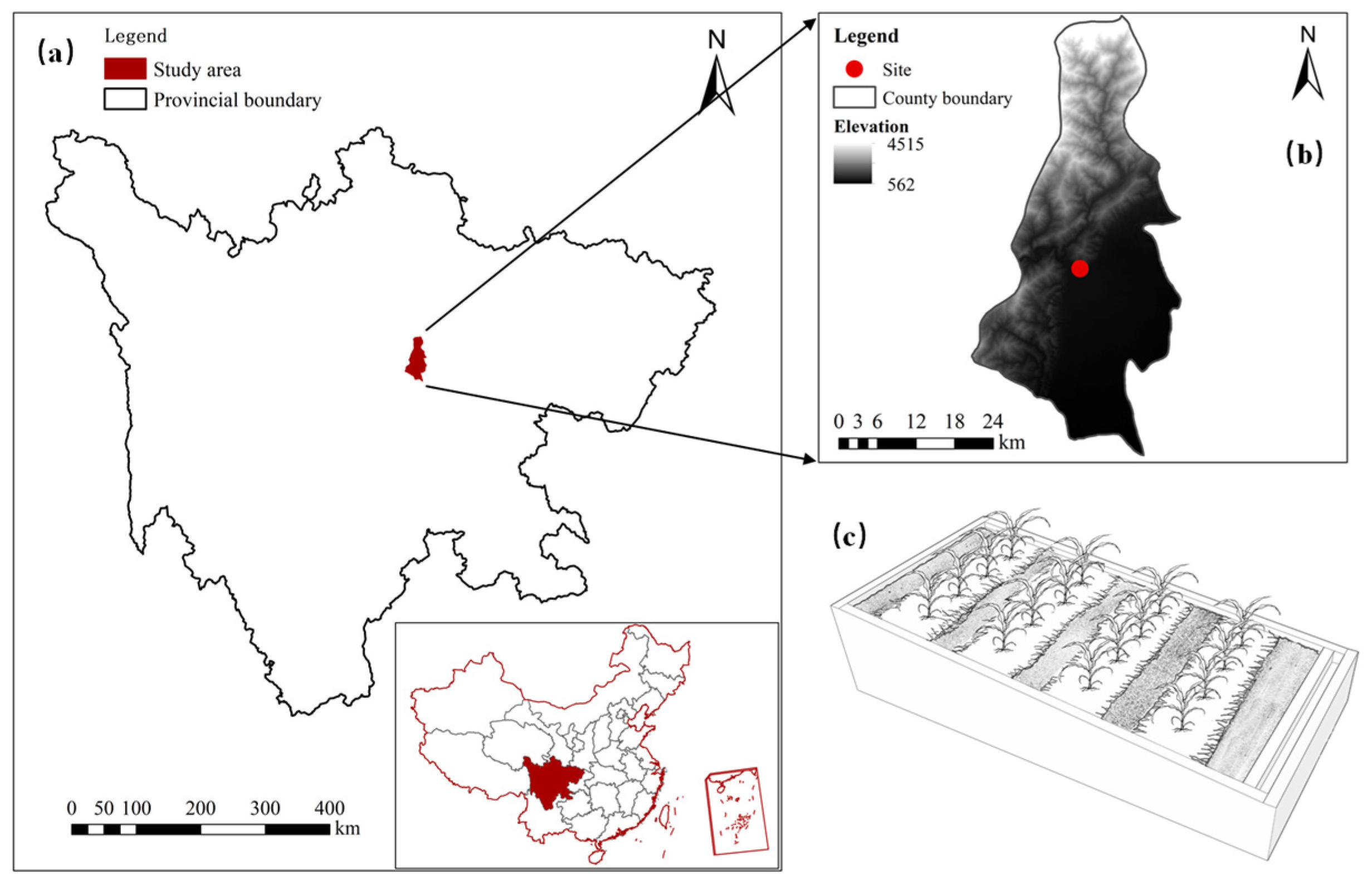
2.1. Study Area

The field experiments were conducted at the research base of Sichuan Agricultural University (31°0034″ N, 103°3652″ E) in the yellow soil area of southwestern China (Figure 1a,b). The mean elevation was 773.5 m in the study area. This region has a subtropical humid monsoon climate and an average annual precipitation of 1218.4 mm, and 80% of the precipitation falls approximately between May and September. According to the USDA soil taxonomy, the soil type is yellow soil, classified as an Ultisol [35], which is susceptible to erosion.

2.2. Experimental Design and Data Acquisition

To record the rainfall, runoff, and soil loss, six experimental field plots with a 15° slope gradient were established in 2014 (Figure 1c).
Each plot had a length of 4 m and width of 2 m, and cross-ridge tillage, one of the main tillage measures used in the area, was implemented. In April 2015, 30,000 kg/hm2 of organic fertilizer was used as the base fertilizer before sowing. The maize-growing season of each year followed the local farming behaviors within the year. As the maize-growing season overlapped with the rainy season, the daily rainfall, runoff, and soil loss were recorded during the maize-growing season from 2015 to 2020. The rainfall was measured using a rain gauge. The runoff and soil loss were collected after each rainfall, and the runoff was determined using the volumetric method; then, the mixture was oven-dried at 105 °C to measure the soil loss. Detailed information on the maize-growing season from 2015 to 2020 is presented in Table 1.

2.3. Methods

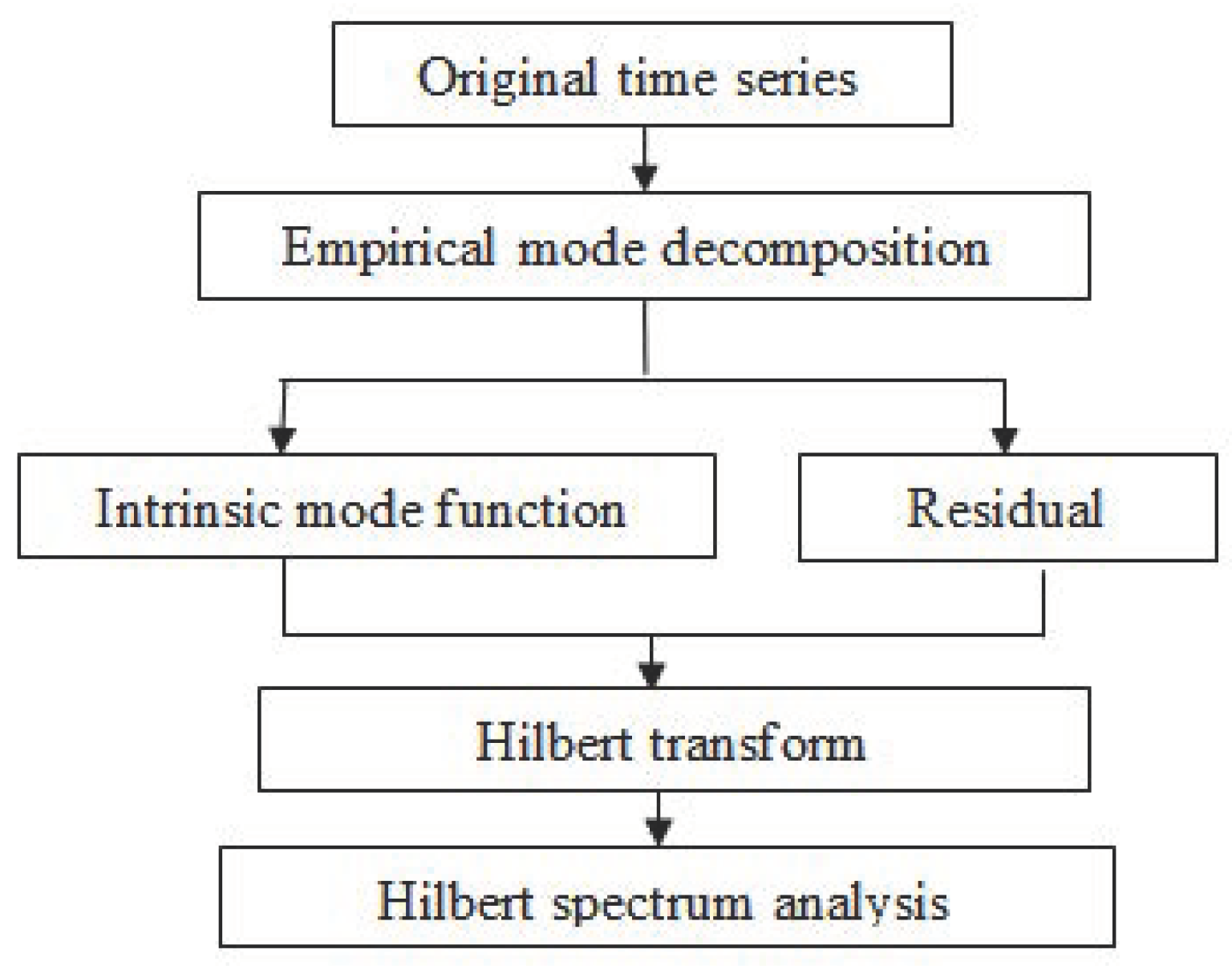
2.3.1. Hilbert–Huang Transform

The HHT comprises two parts: EMD and HSA. EMD uses an adaptive dyadic filter bank to decompose input data into several IMFs and extract a residue representing the trend of the original time series. Sifting is completed when the last component is monotonic or constant, as in this case, where no additional IMFs can be extracted [15,19,33]. The flowchart (Figure 2) and equation for the HHT are as follows:
X ( t ) = k = 1 n I M F k ( t ) + R ( t )
where R(t) is the residue, k represents the numerical value of each sequential IMF, and n is the number of IMFs.
The IMFs indicate the different scales of the original time series and form the physical basis of the data [19,30]. An IMF must satisfy the two conditions to represent a proper output [19]. Additional information on the detailed sifting process of EMD can be found in Massei and Fournier (2012) [13]. However, one of the main problems of the EMD algorithm is mode mixing [33], which likely alters the interpretation of the physical meaning of each IMF. To avoid this drawback, Huang and Wu (2008) [20] proposed the EEMD algorithm, which adds white noise to the original data; the white noise can eventually be removed by averaging the components during the decomposition process.
The mean period (T) of each mode can be calculated [31]. The variance contribution (VC, %) indicates the percent contribution of each IMF to the overall variation of the time series and can be computed as follows [6]:
V C = V k / k = 1 n V k + R
where Vk is the variance of each IMF and residue (R).
The second part is of the HHF is the HSA. The instantaneous frequency of each IMF is obtained by the Hilbert transform [19], and then the Hilbert spectrum (H (θ, t)) can be plotted based on Equation (2) [15]. The Hilbert spectrum can visualize the distribution of the signal amplitude through time and frequency [36], revealing additional properties of the original time series.

2.3.2. Time-Dependent Intrinsic Correlation (TDIC)

Natural processes include various local correlations (positive or negative) with influential factors over time, and the classical method (e.g., Pearson correlation) can only reveal the global relationship, leading to the ignorance of important local correlation information between time series to some extent [31]. Thus, the new TDIC technique was introduced by Chen et al. (2010) [30]. TDIC determines the sliding window size using the instantaneous periods of IMFs based on the EMD algorithm as follows:
R i ( t k / t w ) = C o r r ( I M F i 1 ( t w ) I M F i 2 ( t w ) )
t w = t k t d / 2 : t k + t d / 2
t d = max ( I P i 1 ( t k ) , I P i 2 ( t k ) )
where IPij is the instantaneous period of each IMF, and tw is the adaptive sliding window size. Corr(…) is the cross-correlation coefficient of two time series, and tk is the corresponding time [29].

2.4. Statistical Analysis

The EEMD, Hilbert transform, and TDIC algorithms were executed in MATLAB R2018a (MathWorks. Inc., Reddick, MA, USA). The descriptive statistics and cross-correlation analysis (Pearson correlation) were processed via Microsoft Excel 2016 and SPSS 22.0, respectively.

3. Results and Discussion

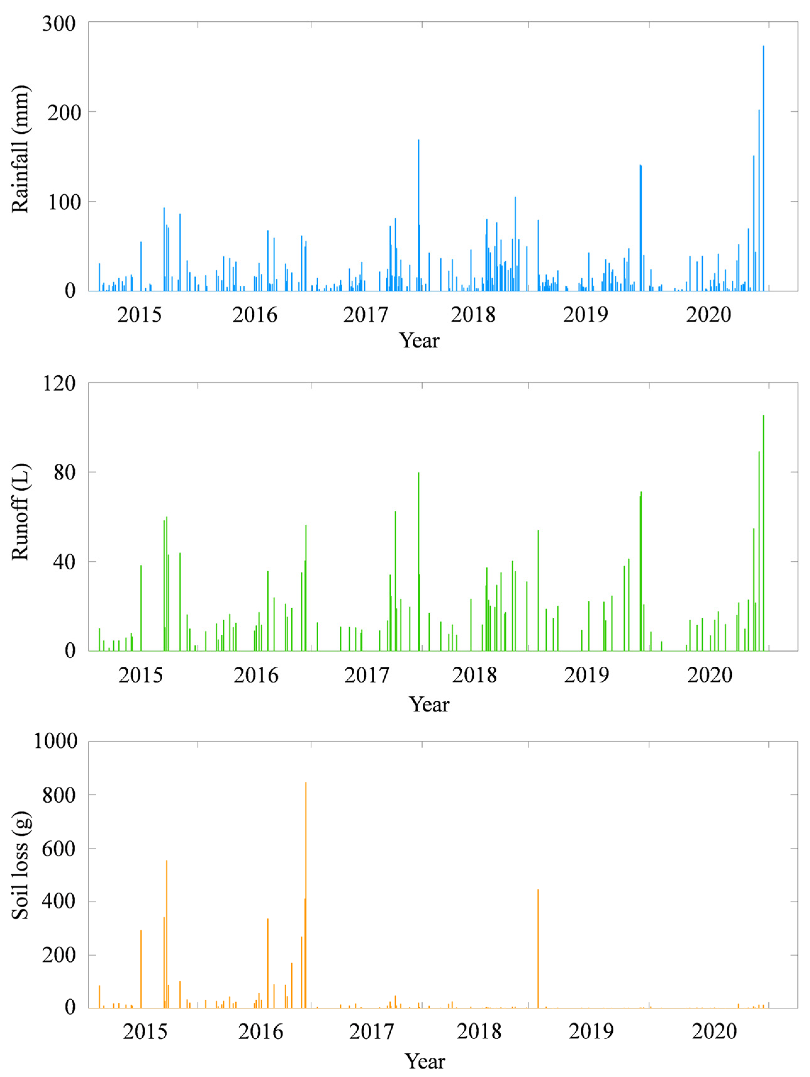
3.1. Descriptive Statistical Analysis of the Original Time Series

Table 2 presents the statistical characteristics of the original time series of rainfall, runoff, and soil loss. The rainfall ranged from 0 to 273.27 mm, with a mean value of 7.68 mm. The highest rainfall was observed in August 2020 (Figure 3). The coefficient of variation (CV) was 281.77%, indicating that rainfall was strongly temporally variable during the maize-growing seasons from 2015 to 2020. The runoff and soil loss ranged from 0 to 105.42 L and 0 to 847.67 g, and the mean values were 3.15 L and 6.63 g, respectively. The highest values of runoff and soil loss were observed in August 2020 and August 2016, respectively. The CVs of the runoff and soil loss, at 339.76% and 739.61%, respectively, indicated that both the runoff and soil loss showed considerable temporal variation during the different maize-growing seasons in 2015–2020. The strong temporal variations were probably caused by the impacts of rainfall and agricultural land use.

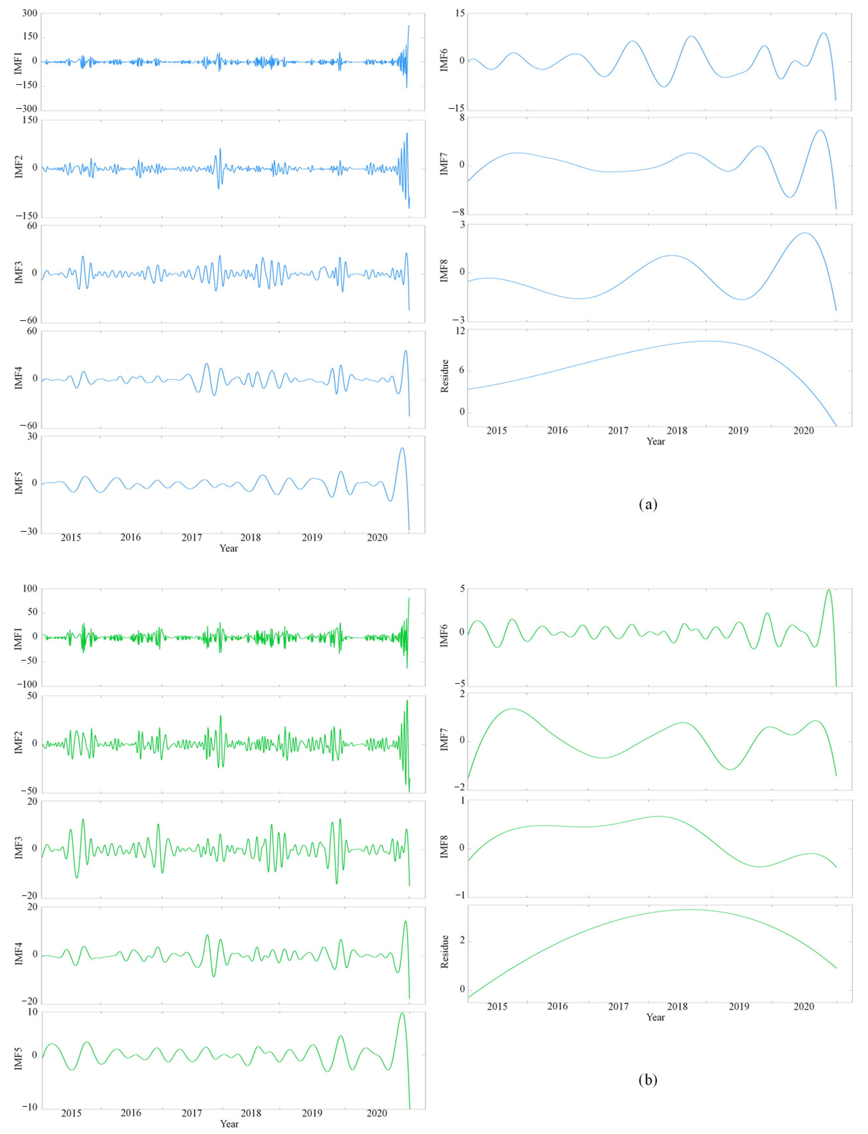
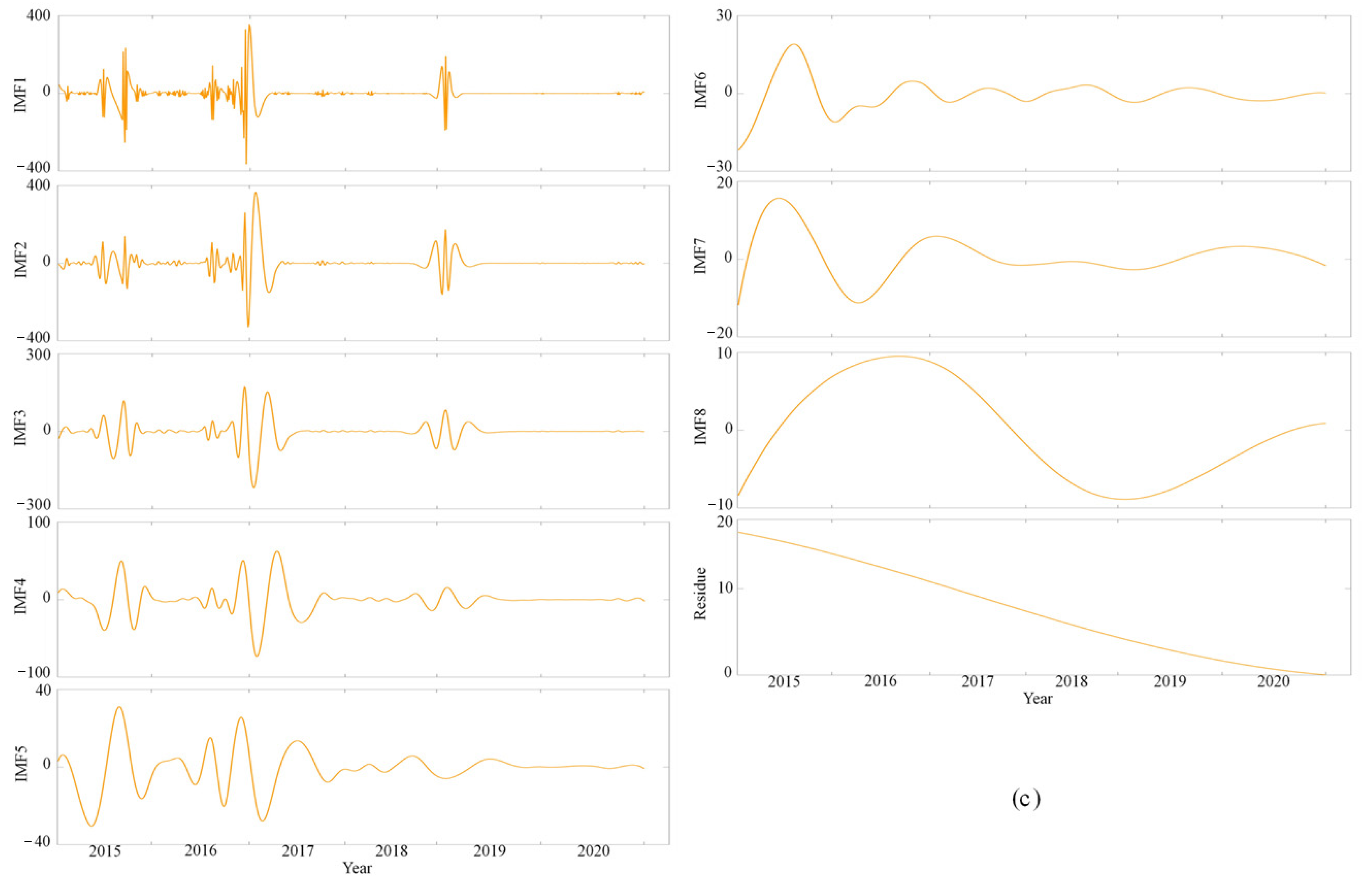
3.2. Ensemble Empirical Mode Decomposition (EEMD)

After using EEMD, the original time series of the rainfall, runoff and soil loss were decomposed into eight IMFs and one residue (Figure 4). Such scales associated with IMFs, if separated clearly, are physically meaningful [37]. For all IMFs, IMF1 has the highest frequency and amplitude, whereas IMF8 oscillates with the lowest frequency and amplitude. That is, the frequency and amplitude of the IMFs decrease as the EEMD algorithm proceeds. The IMFs with lower numerical values separate the higher-frequency oscillations at short-term scales from the lower-frequency oscillations at long-term scales, which correspond to the IMFs with higher numerical values [19]. Liu et al. (2019) [12] obtained ten IMFs for the rainfall, runoff, and suspended sediment concentration (SSC) in the Loess Plateau; these were different from the current results. The SSC is highly nonlinear and uneven at various temporal scales [38,39]. The difference could be attributed to the time series of the rainfall, runoff, and SSC they interpreted, which showed more complexity [6]. The residue showed a predominant trend over time; this was not clearly discerned from the original time series, owing to the nonlinear and nonstationary characteristics of the data [15].
As shown in Figure 4, the residues of rainfall and runoff both showed a trend of increasing and then decreasing, whereas the residue of the soil loss decreased continuously from 2015 to 2020. The results were confirmed by the findings of recent research conducted in southwestern China, wherein soil erosion exhibited a notable declining trend from 1980 to 2015 [40]. Liu et al. (2019) [12] also found that soil erosion showed a substantial decreasing trend in the Loess Plateau from 2006 to 2010, whereas the rainfall and runoff increased and then decreased. This result was likely caused by an increase in soil anti-erodibility and vegetation coverage after maize cultivation [34]. Zhang et al. (2022) [9] highlighted how changes in soil conditions affect soil erosion at long-term scales. Soils with higher soil anti-erodibility are less (or not) susceptible to erosion [41]. Hence, the soil loss showed a decreasing trend over time. In addition, the results confirmed that maize could facilitate soil conservation in this area, as reported in previous studies [24,42].
Table 3 shows the mean periods (T) and variance contributions (VC) of all of the IMFs. The T values of the rainfall IMFs lag behind those of the runoff IMFs and soil loss IMFs. The T of the runoff is nearly equivalent to that of the soil loss for IMF1–IMF2, whereas it is lower for IMF3–IMF8. This result does not agree with Liu et al. (2019) [12], who reported that the periods of the IMFs corresponding to rainfall were generally consistent with those of the runoff and SSC in the Loess Plateau. This discrepancy may be attributed to the soil type and tillage measures. In particular, Ultisols (such as yellow soil) have higher clay content and water-stable aggregate content than Inceptisols (such as Loess soil), providing the Ultisols with stronger water retention and soil anti-erodibility [43]. Therefore, additional time was needed to generate the runoff and subsequent soil loss in the study area. Moreover, we implemented cross-ridge tillage on the sloping farmland. This can increase the topographic relief and restrain runoff behaviors so as to control the occurrences of soil and water loss [16,44]. Furthermore, we found that the periods of rainfall, runoff, and soil loss show significant differences at the IMF8 scale relative to the other scales. The time interval corresponding to the rainfall, runoff, and soil loss may be responsible for this result. Because not all rainfall can cause runoff and soil loss [8], the time intervals for the rainfall, runoff, and soil loss were not equivalent; this may have caused some scale overlaps during decomposition, magnifying the difference in the time scales to some extent [45]. Moreover, Zhang et al. (2022) [9] also obtained similar results and attributed this phenomenon to human activities. Table 3 lists the VC of each IMF. It can be seen that the components at the 0.06 gs scale and 0.15 gs scale corresponding to the rainfall, runoff and soil loss account for nearly 80% of the total variability. Thus, the oscillations of the high-frequency scales play a major role in the variation of the original time series. This result is similar to those found in previous studies [12].
The results highlight that the rainfall, runoff, and soil loss vary the most at the short time scales corresponding to the regional meteorological conditions of the mountainous yellow soil area in southwestern China. Short-duration and high-intensity rainfall can cause a high amount of soil and water loss, but it is infrequent and concentrated within a specific period (Figure 3). Small-sum and low-intensity rainfalls occur most frequently, and such successive events cause soil saturation, leading to repeated runoff and soil loss [8,46]. Gil et al. (2021) [8] also obtained a similar conclusion by analyzing a thirty-year time series from plot studies of mountainous agricultural slopes in the Western Polish Carpathians. Moreover, high amplitudes are observed in the late maize-growing season of each year in IMF4 (mean period of 1 gs). We can infer that the IMF4 of the rainfall represents the concentrated rainfall with a theoretical period of 1 gs occurring in the late maize-growing season (July to August). Therefore, the IMF4 for the runoff and soil loss may represent the corresponding soil and water loss events induced by concentrated rainfall with high intensity. The study area belongs to the rain screen area of West China, which has the characteristics of high precipitation frequency and heavy rainfall, thereby corresponding to the regional meteorological conditions [34].

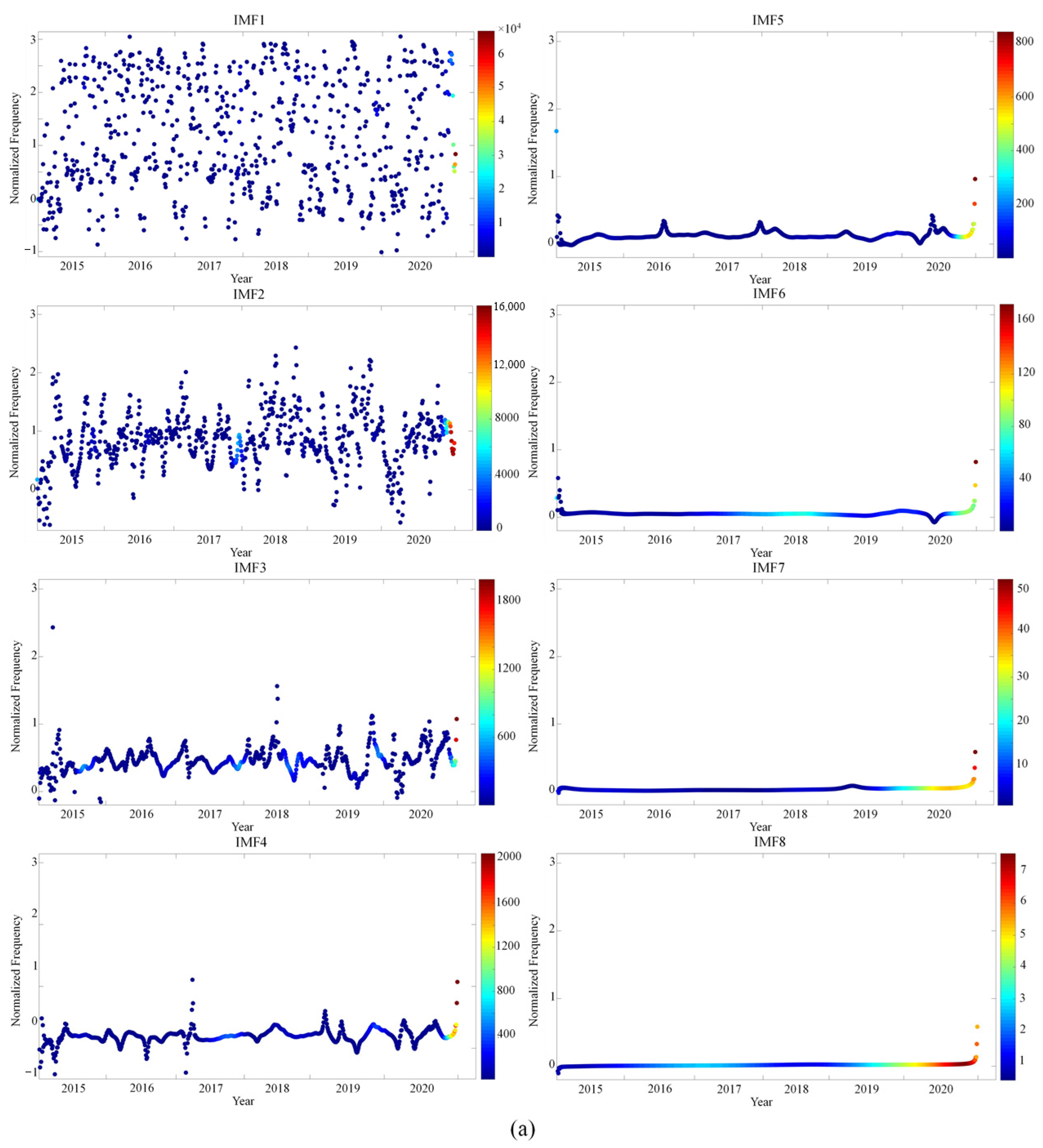
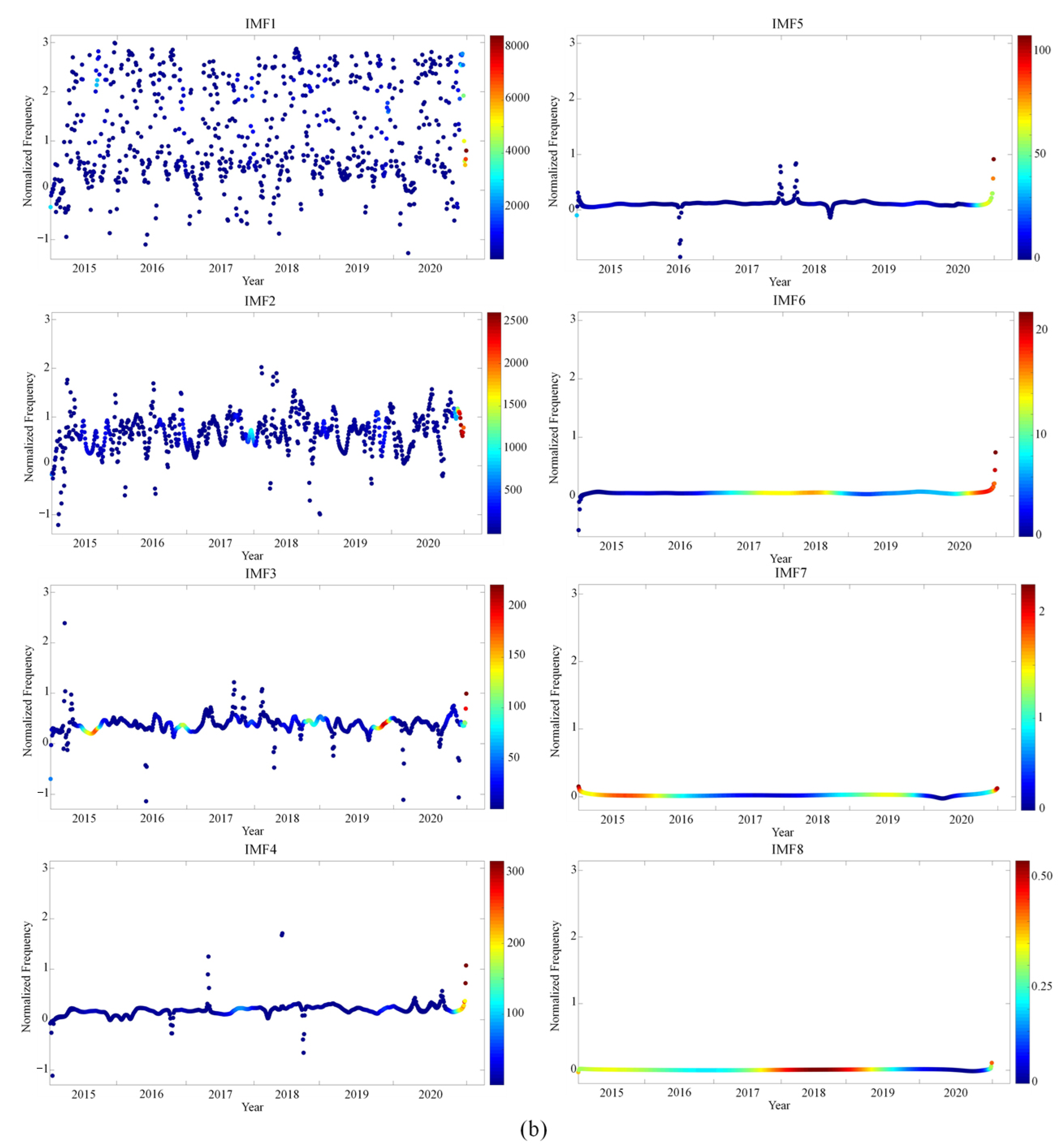
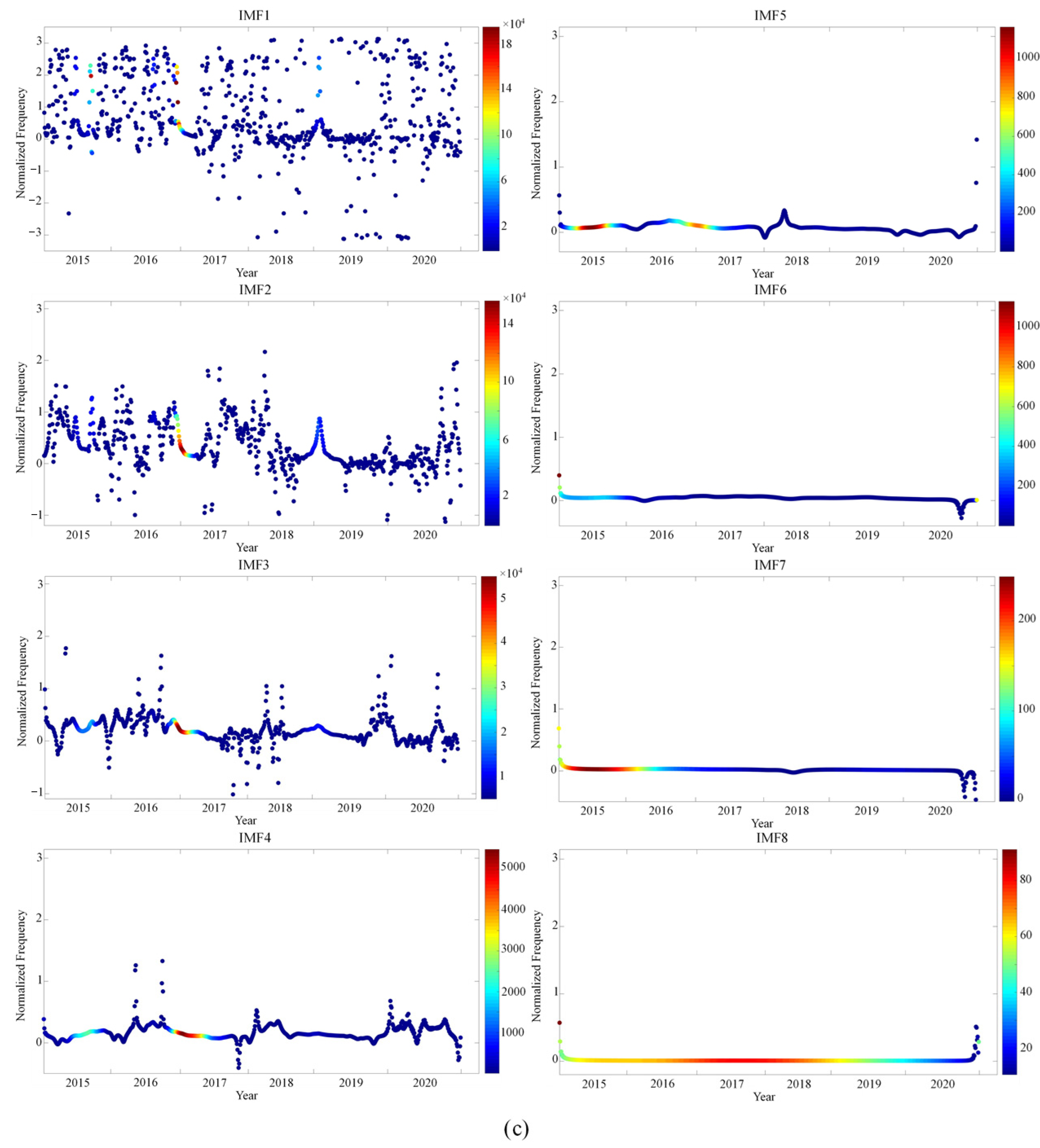
3.3. Hilbert Spectral Analysis (HSA)

The Hilbert spectrum can provide users with insights into the temporal changes in amplitude for each component of a signal by visualizing a three-dimensional plot with respect to time and frequency [13,15]. In these spectra, the y-axis and x-axis provide the variability of the frequency over time [13]; the color scale represents the distribution of the amplitude with time and frequency for each component [12]. In the current study, an intermittent frequency was detected at the high-frequency scales, whereas a continuous frequency was detected at the low-frequency scales; this represented the typical signature of nonlinearity (Figure 5) [36].
The high-frequency components with different amplitudes also indicated the nonstationarity of the original time series [15,19]. For the high-frequency components in this study (IMF1–IMF3), the instantaneous frequency varies with time. The rainfall and runoff show similar spectra, in which high amplitudes are readily detected in the late maize-growing season of 2020 (Figure 5a,b). High amplitudes for soil loss are visible in the late maize-growing season of 2016 (Figure 5c). For the component with a mean period of 1 gs (IMF4), the instantaneous frequency is more regular, and the singularities are quite evident in the form of abrupt changes in the instantaneous frequency, similar to the results from a previous study [13]. Franceschini and Tsai (2010) [36] suggested that this phenomenon likely resulted from natural events or anthropogenic interventions. In addition, high amplitudes can be identified in the late maize-growing season of 2020 for the rainfall and runoff and in the late maize-growing season of 2016 for the soil loss. For the inter-gs scale circulation (IMF5), the frequency is almost constant. The rainfall and runoff exhibit high amplitudes in the late maize-growing season of 2020, whereas the soil loss displays concentrated high amplitudes in the mid-maize-growing season of 2015. Furthermore, the frequency becomes constant at larger scales (IMF6–IMF8). The concentration of the high amplitudes prevails over a long period, particularly in regard to soil loss. This may be related to rainfall characteristics, as well as the interception, stem flow, and root action of maize in different periods in the study area.

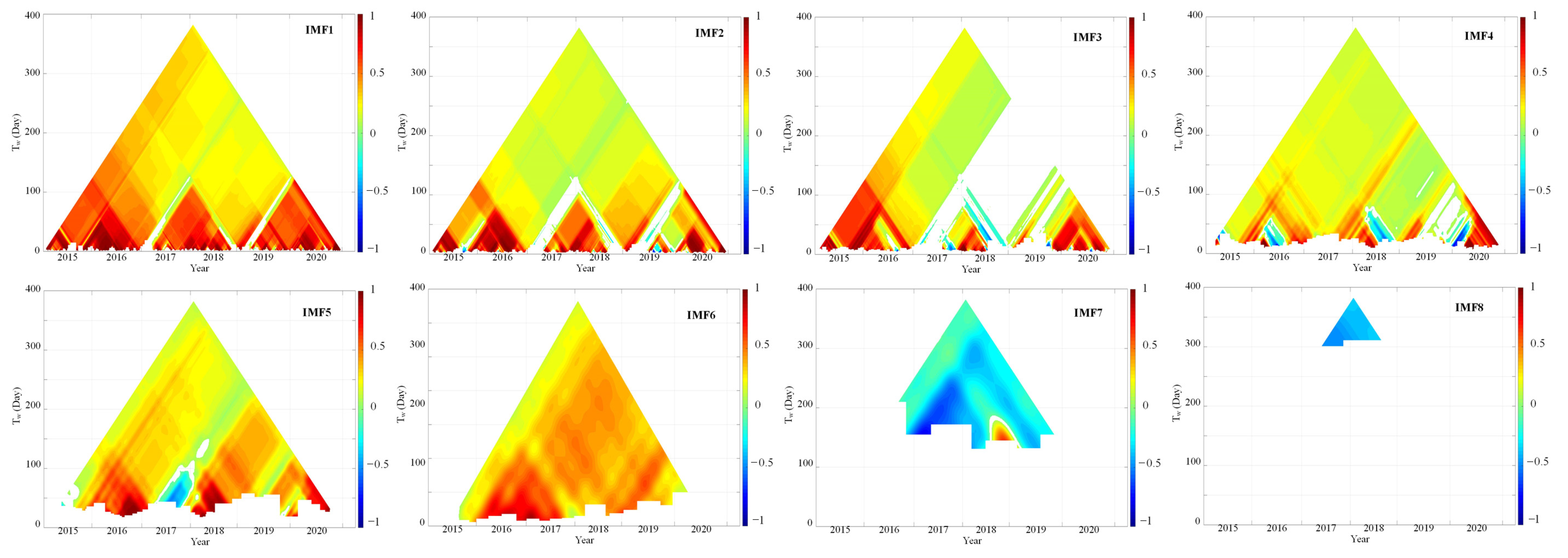
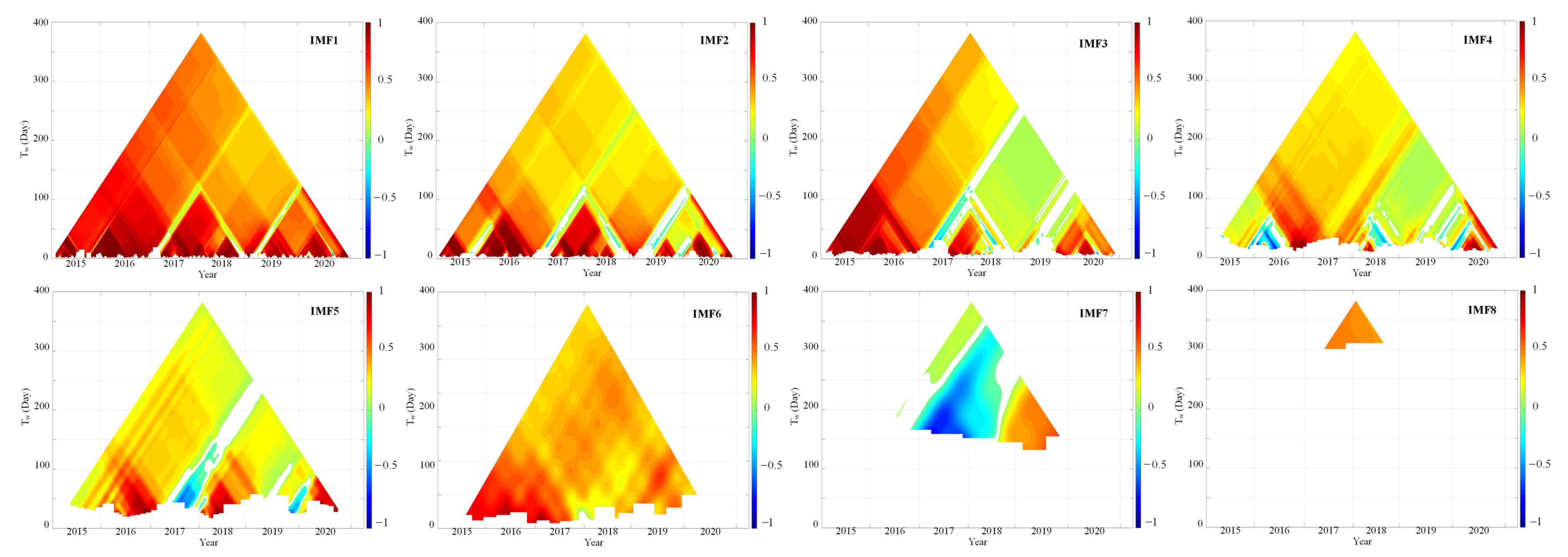
3.4. Global Cross-Correlation Analysis and the TDIC

Time series from natural science fluctuate in a whole range of scales, which may be a result of the fractal nature of physical processes and influencing factors [42,47,47]. Thus, the interpretation must consider the scale question [48]. In particular, a cross-correlation analysis based on multiple scales is necessary to identify the associations between soil loss, rainfall, and runoff. From Table 4, strong and positive correlations are observed in the association between soil loss and rainfall and between soil loss and runoff, but the nature and degree of the correlations are not consistent for the rest of the cases. That is, at short-term scales, the correlation is positive, whereas, at long-term scales, the association can be negative. For example, when considering the correlation between soil loss and rainfall, the correlation coefficients are 0.209 for IMF1 and −0.361 for IMF8. The negative correlations between the soil loss and both rainfall and runoff occur at a large scale, which may be related to the fact that the rainfall and runoff cannot reach the threshold for causing soil loss. At the 1 gs scale (IMF4), the link is relatively weak compared to other scales; this is contrary to common knowledge, i.e., that concentrated rainfall is highly correlated with soil and water loss. This can be explained by the fact that the correlation is determined by the occurrence, development, and mechanisms of operation between variables [42]. The global correlation considers the average over time as defined in an integral sense based on the complete dataset [29]. However, in fact, correlations may show rich dynamics, and strong correlations can be quite local in the time domain [32]. Therefore, the classical cross-correlation, as applied to nonlinear and nonstationary time series, may ignore local correlations and distort the true correlation information between time series, consequently providing misleading interpretations [29,30,46]. Adarsh and Priya (2020) [18] also highlighted that reasonably good correlations should not be ignored in local time periods or time scales, although the global correlation may be very low. To gain greater insight into the local moving correlation between soil erosion and rainfall, a TDIC based on EEMD was employed in our study. In general, the TDIC can calculate the running correlation matrix for IMFs with a similar mean period and generates a graphic triangle. In the TDIC plot, the y-axis and x-axis represent the sliding window size and time, respectively. The color bar indicates the correlation between the two components [29,30].
The measured TDIC between the soil loss and rainfall is presented in Figure 6. There is a predominant positive correlation between the two variables in IMF1 and IMF2, which indicates the strong influence of rainfall on soil loss at short-term scales. Massei and Fournier (2012) [13] highlighted that time scales of less than half a month may represent a rapid response to rainfall that directly results in soil erosion. Small and low-intensity rainfalls occur the most frequently and can repeatedly cause soil saturation and, thus, soil and water loss in mountainous areas [8]. Therefore, it is evident that the high-frequency component of rainfall plays a direct role in the soil loss process. IMF3 exhibits a dominant positive correlation, but during a short period in 2017 and 2018, a negative association can be observed. At the 1 gs scale (IMF4), the rich dynamics of the correlation can be seen over time, and the switchover of positive and negative correlation mainly occurs in the maize-growing seasons of 2016, 2018, and 2020. The reason for such a switchover may be that the rainfall oscillation is not sufficiently large to lead to soil loss when considering the maize cover, especially in the mid-maize-growing season. During this period, the maize cover is so high that it can efficiently protect the soil surface from rainfall; moreover, the maize roots are significantly developed and are therefore able to stabilize the soil structure more effectively than in the early maize-growing season [34]. In addition, the rainfall intensity is smaller than that in the late maize-growing season. Consequently, it is difficult to generate soil loss during the mid-maize-growing season. The switchover of the nature correlation contributes to the low correlation (0.129), as anticipated. IMF5 displays a pronounced negative association during the short time spell of the maize-growing season of 2017, even though the correlation is primarily positive. A constant positive correlation is visible at the IMF6 scale, indicating that rainfall will accelerate soil loss at the 6 gs scale. IMF7 shows a predominant negative correlation, but there is a local positive correlation in 2018–2019. The results reveal a negative relationship on a large scale, potentially related to the impacts of agricultural land use. It is believed that agricultural cultivation can increase soil loss [5,8,49]. However, based on a previous study in the same location [34] and positive feedback regarding the maize growth and application of organic fertilizer, the soil stability in this area has improved over time. Consequently, there is uncertainty about soil loss due to rainfall events. The switchover from a negative to positive correlation can be explained by the fact that during the early maize-growing season of 2019 (26 April), an unexpected rainstorm occurred when the slope was plowed without vegetation cover. Accordingly, a severe soil loss is observed after the rainfall (446.33 g). Moreover, the correlation dynamics are fairly stable at the larger time scales of IMF5; this was also reported in a reservoir inflow study in India [50]. Fluctuations of the long-term scale may be related to seasonal weather, global climate change, and soil conditions in the watershed [12,31]. The results confirm that the global cross-correlation coefficient ignores the local/multi-scale information, which could be recovered by a proper methodology (Chen et al., 2010). Therefore, changes at a large time scale are slow and have a low amplitude, making the correlation more stable.
Figure 7 shows the TDIC between the soil loss and runoff at different temporal scales. A long-range positive correlation is observed in the entire time domain, i.e., not only at short time scales (IMF1, IMF2) but also at long-term scales (IMF6, IMF8). This suggests that the runoff shows stronger impacts and better consistency with the fluctuations of the soil loss at multiple time scales relative to the case with rainfall. Liu et al. (2019) [12] showed a similar result, i.e., that runoff was more strongly correlated with the SSC than with rainfall. IMF7 exhibits a distinct switchover from a negative correlation to a positive correlation during 2018–2019. This result may be related to extreme soil erosion events in April 2019. High heterogeneity is visible in the correlations at the IMF3, IMF4, and IMF5 scales. However, these transformations of the correlations may be owing to uncertain physical processes, such as local microclimates and human intervention [50]. The exact reasons require further investigation in the future. Overall, the TDIC breaks the notion of uniqueness regarding the nature of the association between soil loss, rainfall, and runoff; the relationship varies in time scale and time domain [18]. Based on the TDIC, we can conclude that at some scales, rainfall and runoff are likely not as influential on the soil loss process as at other scales. Therefore, using the TDIC technique to identify such low influential modes at multiple scales and excluding them may eventually improve soil loss prediction performance [12,50].

4. Conclusions

The EEMD-based TDIC method breaks the notion that the correlations between soil loss, rainfall, and runoff are not always unique but vary over time at some scales. Eight IMFs and one residue were obtained by EEMD. Our results showed the soil loss decreased during the growing season of maize from 2015 to 2020, but the rainfall and runoff showed an increasing trend. IMF1–IMF2 accounted for nearly 80% of the temporal variations in rainfall, runoff, and soil loss, indicating that the variables varied the most at short time scales. Small and low-intensity rainfall and the soil loss that occurred as a result occurred most frequently in the yellow soil area of southwestern China. The HSA illustrated that the instantaneous values of each variable varied with time at short time scales but were stable at long-term scales. Strong and positive correlations between soil loss, rainfall, and runoff were observed over the entire period at the IMF1 and IMF2 scales, indicating that such high-frequency rainfall (with a small sum and low intensity) showed a rapid and direct influence on soil loss. The TDIC revealed the evolution of the local correlation between soil loss, rainfall, and runoff with time at the IMF3–IMF5 scales. The switchover from a negative correlation to a positive correlation at the IMF7 scale may be related to a sudden natural event (rainstorm) and/or human intervention (tillage or cultivation). Compared with the traditional correlation between soil loss and runoff, a scale-dependent moving correlation analysis can provide more information with time and frequency. The small and low-intensity rainfalls that were often ignored in previous studies occurred most frequently and showed dominant impacts on inducing soil loss; moreover, the concentrated rainfalls with high intensity were correlated with the soil loss very locally. Thus, greater attention should be paid to soil loss caused by high-frequency rainfall in the study area. A better understanding of the time-varying associations may assist authorities in imposing measures that are more adaptive to local characteristics to control soil loss from sloping farmlands. We suggest that the characteristics of rainfall should be fully considered in the allocation of soil and water conservation measures, especially high-frequency rainfall in the study area.

Author Contributions

X.S.: conceptualization, methodology, software, data curation, visualization, writing—original draft, writing—review and editing. S.H.: conceptualization, funding acquisition, project administration, investigation, writing—review and editing. R.M.: conceptualization, methodology, software, data curation, visualization, writing—original draft. Z.Z.: conceptualization, methodology, investigation, formal analysis, funding acquisition, project administration, writing—review and editing. H.Y.: writing—review and editing. X.L.: writing—review and editing. All authors have read and agreed to the published version of the manuscript.

Funding

This research was financially supported by the National Natural Science Foundation (No. 42177316) and the Sichuan Key Research and Development Program (2019YFS0463).

Data Availability Statement

Data from this work are available upon request.

Acknowledgments

The authors express their gratitude to Liu, Q.J. and Zhang, H.Y. for their help with EEMD codes. The authors thank Huang, Y.X. for providing the basic source codes of TDIC with the intention of promoting noncommercial scientific research (https://zenodo.org/record/9748#.XBhUF2lS-Uk (accessed on 6 July 2020)).

Conflicts of Interest

The authors declare no conflict of interest.

References

  1. Xiong, M.Q.; Sun, R.H.; Chen, L.D. Effects of soil conservation techniques on water erosion control: A global analysis. Sci. Total. Environ. 2018, 645, 753–760. [Google Scholar] [CrossRef] [PubMed]
  2. Chen, J.; Xiao, H.B.; Li, Z.W.; Liu, C.; Ning, K.; Tang, C.J. How effective are soil and water conservation measures (SWCMs) in reducing soil and water losses in the red soil hilly region of China? A meta-analysis of field plot data. Sci. Total Environ. 2020, 735, 139517. [Google Scholar] [CrossRef] [PubMed]
  3. Wang, H.; Zhang, G.H. Temporal variation in soil erodibility indices for five typical land use types on the Loess Plateau of China. Geoderma 2021, 381, 114695. [Google Scholar] [CrossRef]
  4. Zhang, B.J.; Zhang, G.H.; Zhu, P.Z.; Yang, H.Y. Temporal variations in soil erodibility indicators of vegetation-restored steep gully slopes on the Loess Plateau of China. Agric. Ecosyst. Environ. 2019, 286, 106661. [Google Scholar] [CrossRef]
  5. Han, J.Q.; Ge, W.Y.; Hei, Z.; Cong, C.Y.; Ma, C.L.; Xie, M.X.; Liu, B.Y.; Feng, W.; Wang, F.; Jiao, J.Y. Agricultural land use and management weaken the soil erosion induced by extreme rainstorms. Agric. Ecosyst. Environ. 2020, 301, 107047. [Google Scholar] [CrossRef]
  6. Adarsh, S.; Janga Reddy, M. Analysing the variability of streamflow and suspended sediment concentration using time dependent intrinsic correlation. Procedia Technol. 2016, 24, 54–61. [Google Scholar]
  7. Wen, X.; Deng, X.Z. Current soil erosion assessment in the Loess Plateau of China: A mini-review. J. Clean. Prod. 2020, 276, 123091. [Google Scholar] [CrossRef]
  8. Gil, E.; Kijowska-Strugała, M.; Demczuk, P. Soil erosion dynamics on a cultivated slope in the Western Polish Carpathians based on over 30 years of plot studies. Catena 2021, 207, 105682. [Google Scholar] [CrossRef]
  9. Zhang, H.Y.; Liu, L.; Jiao, W.; Li, K.; Wang, L.Z.; Liu, Q.J. Watershed runoff modeling through a multi-time scale approach by multivariate empirical mode decomposition (MEMD). Environ. Sci. Pollut. Res. 2022, 29, 2819–2829. [Google Scholar] [CrossRef]
  10. Hu, W.; Si, B.C. Soil water prediction based on its scale-specific control using multivariate empirical mode decomposition. Geoderma 2013, 193–194, 180–188. [Google Scholar] [CrossRef]
  11. Huang, S.Z.; Chang, J.X.; Huang, Q.; Chen, Y.T. Monthly streamflow prediction using modified EMD-based support vector machine. J. Hydrol. 2014, 511, 764–775. [Google Scholar] [CrossRef]
  12. Liu, Q.J.; Zhang, H.Y.; Gao, K.T.; Xu, B.; Wu, J.Z.; Fang, N.F. Time-frequency analysis and simulation of the watershed suspended sediment concentration based on the Hilbert-Huang transform (HHT) and artificial neural network (ANN) methods: A case study in the Loess Plateau of China. Catena 2019, 179, 107–118. [Google Scholar] [CrossRef]
  13. Massei, N.; Fournier, M. Assessing the expression of large-scale climatic fluctuations in the hydrological variability of daily Seine river flow between 1950 and 2008 using Hilbert–Huang Transform. J. Hydrol. 2012, 448–449, 119–128. [Google Scholar] [CrossRef]
  14. Huang, N.E.; Shen, S.S.P. Hilbert-Huang Transform and Its Application, 2nd ed.; World Scientific Publishing Company: Singapore, 2014. [Google Scholar]
  15. Tsai, C.W.; Treadwell, H. Analysis of trends and variability of toxic concentrations in the Niagara River using the Hilbert-Huang transform method. Ecol. Inform. 2019, 51, 129–150. [Google Scholar] [CrossRef]
  16. Luo, J.; Zheng, Z.C.; Li, T.X.; He, S.Q. Temporal variations in runoff and sediment yield associated with soil surface roughness under different rainfall patterns. Geomorphology 2020, 349, 106915. [Google Scholar] [CrossRef]
  17. Luo, J.; Zheng, Z.C.; Li, T.X.; He, S.Q.; Zhang, X.Z.; Huang, H.G.; Wang, Y.D. Quantifying the contributions of soil surface microtopography and sediment concentration to rill erosion. Sci. Total Environ. 2021, 752, 141886. [Google Scholar] [CrossRef]
  18. Adarsh, S.; Priya, K.L. Multiscale running correlation analysis of water quality datasets of Noyyal River, India, using the Hilbert–Huang Transform. Int. J. Environ. Sci. Technol. 2020, 17, 1251–1270. [Google Scholar] [CrossRef]
  19. Huang, N.E.; Shen, Z.; Long, S.R.; Wu, M.C.; Shih, H.H.; Zheng, Q.; Yen, N.C.; Tung, C.C.; Liu, H.H. The empirical mode decomposition and the Hilbert spectrum for nonlinear and non-stationary time series analysis. Proc. Roy. Soc. A Math. Phys. Eng. Sci. 1998, 454, 903–995. [Google Scholar] [CrossRef]
  20. Huang, N.E.; Wu, Z.H. A review on Hilbert-Huang transform: Method and its applications to geophysical studies. Rev. Geophys. 2008, 46, 1–23. [Google Scholar] [CrossRef] [Green Version]
  21. O’Hara, S.L.; Street-Perrott, F.A.; Burt, T.P. Climate change and soil erosion. Nature 1993, 364, 197. [Google Scholar] [CrossRef]
  22. Liang, Y.; Jiao, J.Y.; Tang, B.Z.; Cao, B.T.; Li, H. Response of runoff and soil erosion to erosive rainstorm events and vegetation restoration on abandoned slope farmland in the Loess Plateau region, China. J. Hydrol. 2020, 584, 124694. [Google Scholar]
  23. Anache, J.A.A.; Wendland, E.C.; Oliveria, P.T.S.; Flanagan, D.C.; Nearing, M.A. Runoff and soil erosion plot-scale studies under natural rainfall: A meta-analysis of the Brazilian experience. Catena 2017, 152, 29–39. [Google Scholar] [CrossRef]
  24. Luo, J.; Zheng, Z.C.; Li, T.X.; He, S.Q. The changing dynamics of rill erosion on sloping farmland during the different growth stages of a maize crop. Hydrol. Process. 2019, 33, 76–85. [Google Scholar] [CrossRef] [Green Version]
  25. Wang, Y.; Luo, J.; Zheng, Z.C.; Li, T.X.; He, S.Q.; Zhang, X.Z.; Wang, Y.D.; Liu, T. Assessing the contribution of the sediment content and hydraulics parameters to the soil detachment rate using a flume scouring experiment. Catena 2019, 176, 315–323. [Google Scholar] [CrossRef]
  26. Polyakov, V.O.; Nearing, M.A.; Stone, J.J. Soil loss from small rangeland plots under simulated rainfall and run-on conditions. Geoderma 2020, 361, 114070. [Google Scholar] [CrossRef]
  27. Fang, N.F.; Shi, Z.H.; Li, L.; Guo, Z.L.; Liu, Q.J.; Ai, L. The effects of rainfall regimes and land use changes on runoff and soil loss in a small mountainous watershed. Catena 2012, 99, 1–8. [Google Scholar] [CrossRef]
  28. Naqvi, H.R.; Mohammed Abdul Athick, A.S.; Siddiqui, L.; Siddiqui, M.A. Multiple modeling to estimate sediment loss and transport capacity employing hourly rainfall and In-Situ data: A prioritization of highland watershed in Awash River basin, Ethiopia. Catena 2019, 182, 104173. [Google Scholar] [CrossRef]
  29. Plocoste, T.; Calif, R.; Jacoby-Koaly, S. Multi-scale time dependent correlation between synchronous measurements of ground-level ozone and meteorological parameters in the Caribbean Basin. Atmos. Environ. 2019, 211, 234–246. [Google Scholar] [CrossRef]
  30. Chen, X.Y.; Wu, Z.H.; Huang, N.E. The time-dependent intrinsic correlation based on the empirical mode decomposition. Adv. Adap. Data Anal. 2010, 2, 233–265. [Google Scholar] [CrossRef]
  31. Huang, Y.X.; Schmitt, F.G.; Lu, Z.M.; Liu, Y.L. Analysis of daily river flow fluctuations using empirical mode decomposition and arbitrary order Hilbert spectral analysis. J. Hydrol. 2009, 373, 103–111. [Google Scholar] [CrossRef] [Green Version]
  32. Kbaier Ben Ismail, D.; Lazure, P.; Puillat, I. Statistical properties and time-frequency analysis of temperature, salinity and turbidity measured by the MAREL Carnot station in the coastal waters of Boulogne-sur-Mer. J. Marine. Syst. 2016, 162, 137–153. [Google Scholar] [CrossRef] [Green Version]
  33. Tsai, C.W.; Hsiao, Y.R.; Lin, M.L.; Hsu, Y.W. Development of a noise-assisted multivariate empirical mode decomposition framework for characterizing PM 2.5 air pollution in Taiwan and its relation to hydro-meteorological factors. Environ. Int. 2020, 139, 105669. [Google Scholar] [CrossRef] [PubMed]
  34. Ma, R.; Zheng, Z.C.; Li, T.X.; He, S.Q.; Zhang, X.Z.; Wang, Y.D.; Huang, H.G.; Ye, D.H. Temporal variation of soil erosion resistance on sloping farmland during the growth stages of maize (Zea mays L.). Hydrol. Process. 2021, 35, e14353. [Google Scholar] [CrossRef]
  35. Soil Survey Staff. Keys to Soil Taxonomy, 12th ed.; United States Department of Agriculture, Natural Resources Conservation Service: Washington, DC, USA, 2014.
  36. Franceschini, S.; Tsai, C.W. Application of Hilbert-Huang Transform method for analyzing toxic cdoncentrations in the Niagara River. J. Hydrol. Eng. 2010, 15, 90–96. [Google Scholar] [CrossRef]
  37. Looney, D.; Hemakom, A.; Mandic, D.P. Intrinsic multi-scale analysis: A multi-variate empirical mode decomposition framework. Proc. R. Soc. A 2015, 471, 20140709. [Google Scholar] [CrossRef] [PubMed] [Green Version]
  38. Kuai, K.Z.; Tsai, C.W. Identification of varying time scales in sediment transport using the Hilbert–Huang Transform method. J. Hydrol. 2012, 420–421, 245–254. [Google Scholar] [CrossRef]
  39. Zheng, M.; Qin, F.; Yang, J.; Cai, Q. The spatio-temporal invariability of sediment concentration and the flow-sediment relationship for hilly areas of the Chinese Loess Plateau. Catena 2013, 109, 164–176. [Google Scholar] [CrossRef]
  40. Gao, J.B.; Wang, H. Temporal analysis on quantitative attribution of karst soil erosion: A case study of a peak-cluster depression basin in Southwest China. Catena 2019, 172, 369–377. [Google Scholar] [CrossRef]
  41. Dou, Y.X.; Yang, Y.; An, S.S.; Zhu, Z.L. Effects of different vegetation restoration measures on soil aggregate stability and erodibility on the Loess Plateau, China. Catena 2020, 185, 104294. [Google Scholar] [CrossRef]
  42. Shen, H.O.; He, Y.F.; Hu, W.; Geng, S.B.; Han, X.; Zhao, Z.J.; Li, H.L. The temporal evolution of soil erosion for corn and fallow hillslopes in the typical Mollisol region of Northeast China. Soil. Tillage Res. 2019, 186, 200–205. [Google Scholar] [CrossRef]
  43. Chen, M.Q.; Zhang, Z.D.; Wang, X.L.; Zhang, K.L.; Chen, Y.H. A comparison of slope erosion sediment yield characteristics of yellow soil in Southwest China and loess in Northwest China. Sci. Soil Water Conser. 2016, 14, 53–60. (In Chinese) [Google Scholar]
  44. Guo, S.F.; Zhai, L.M.; Liu, J.; Liu, H.B.; Chen, A.Q.; Wang, H.Y.; Wu, S.X.; Lei, Q.L. Cross-ridge tillage decreases nitrogen and phosphorus losses from sloping farmlands in southern hilly regions of China. Soil. Tillage Res. 2019, 191, 48–56. [Google Scholar] [CrossRef]
  45. Zhu, X.C.; Liang, Y.; Tian, Z.Y.; Wang, X. Analysis of scale-specific factors controlling soil erodibility in southeastern China using multivariate empirical mode decomposition. Catena 2021, 199, 105131. [Google Scholar] [CrossRef]
  46. Hirmas, D.R.; Giménez, D.; Nemes, A.; Kerry, R.; Brunsell, N.A.; Wilson, C.J. Climate-induced changes in continental-scale soil macroporosity may intensify water cycle. Nature 2018, 561, 100–103. [Google Scholar] [CrossRef] [PubMed]
  47. She, D.L.; Chen, Q.; Luis, C.T.; Samuel, B.; Hu, W.; Tamara, L.C.; Luciana, M.O. Multi-scale correlations between soil hydraulic properties and associated factors along a Brazilian watershed transect. Geoderma 2017, 286, 15–24. [Google Scholar]
  48. Huang, Y.X.; Schmitt, F.G. Time dependent intrinsic correlation analysis of temperature and dissolved oxygen time series using empirical mode decomposition. J. Mar. Syst. 2014, 130, 90–100. [Google Scholar] [CrossRef] [Green Version]
  49. Li, Z.W.; Ning, K.; Chen, J.; Liu, C.; Wang, D.Y.; Nie, X.D.; Hu, X.Q.; Wang, L.X.; Wang, T.W. Soil and water conservation effects driven by the implementation of ecological restoration projects: Evidence from the red soil hilly region of China in the last three decades. J. Clean. Prod. 2020, 260, 121109. [Google Scholar] [CrossRef]
  50. Adarsh, S.; Janga Reddy, M. Multiscale characterization and prediction of reservoir inflows using MEMD-SLR coupled approach. J. Hydrol. Eng. 2019, 24, 04018059. [Google Scholar] [CrossRef]
Figure 1. Location of the study area in Sichuan Province: (a) experimental plot in Dujiangyan County (b) and schematic diagram of experimental plot (c).
Agronomy 13 01492 g001
Figure 2. Schematic diagram of HHT.
Agronomy 13 01492 g002
Figure 3. Original data of rainfall, runoff, and soil loss.
Agronomy 13 01492 g003
Figure 4. Intrinsic mode functions (IMF) and residues of rainfall (a), runoff (b), and soil loss (c) during the maize-growing seasons from 2015 to 2020 determined by EEMD.
Agronomy 13 01492 g004aAgronomy 13 01492 g004b
Figure 5. Hilbert spectrum of rainfall (a), runoff (b), and soil loss (c). The color scale depicts the amplitude of each IMF.
Agronomy 13 01492 g005aAgronomy 13 01492 g005bAgronomy 13 01492 g005c
Figure 6. Measured TDIC between rainfall and soil loss. The white space of the plot indicates that the correlation cannot pass the t-test at the 95% level.
Agronomy 13 01492 g006
Figure 7. Measured TDIC between the soil loss and runoff. The white space of the plot indicates that the correlation cannot pass the t-test at 95% level.
Agronomy 13 01492 g007
Table 1. Recorded information on each maize-growing season from 2015 to 2020.
YearStarting DateEnding DateDuration (Days)
20156th May5th September123
201616th April21st August128
201719th April21st August125
201818th April15th August120
201916th April29th August136
20209th April21st August135
Table 2. Descriptive statistics of rainfall, runoff, and soil loss.
MinimumMaximumMeanSDCV (%)Skewness
Rainfall (mm)0273.277.6821.63281.775.85
Runoff (L)0105.423.1510.70339.764.89
Soil loss (g)0847.676.6349.05739.6111.46
Note: SD, standard deviation; CV, coefficient of variation.
Table 3. The corresponding mean period T (expressed in the mean maize-growing season, gs) and variance contribution VC (%) of each IMF of rainfall, runoff, and soil loss.
IMFsRainfallRunoffSoil Loss
TVCTVCTVC
IMF10.0553.730.0652.490.0630.97
IMF20.1127.950.1531.210.1540.84
IMF30.286.140.367.520.4421.37
IMF40.946.390.784.391.303.96
IMF52.062.432.261.613.191.33
IMF66.031.748.981.959.120.45
IMF715.870.5020.910.2422.330.38
IMF837.580.1664.770.0689.320.32
Residue0.960.520.36
Table 4. Global cross-correlation coefficients between soil loss with rainfall and runoff for the IMFs and residues after EEMD.
RainfallRunoff
IMF10.209 **0.399 **
IMF20.124 **0.258 **
IMF30.188 **0.380 **
IMF40.129 **0.198 **
IMF50.113 **0.139 **
IMF60.142 **0.274 **
IMF7−0.083 *0.155 **
IMF8−0.361 **0.449 **
Residue−0.208 **−0.539 **
Note: * p < 0.05, ** p < 0.01, n = 767.
Disclaimer/Publisher’s Note: The statements, opinions and data contained in all publications are solely those of the individual author(s) and contributor(s) and not of MDPI and/or the editor(s). MDPI and/or the editor(s) disclaim responsibility for any injury to people or property resulting from any ideas, methods, instructions or products referred to in the content.

