Assessing the Convergence of Farming Systems towards a Reduction of Greenhouse Gas Emissions in European Union Countries

Abstract

This study investigates change in the intensification of agricultural activities and its effect on the greenhouse gas (GHG) emissions of the 27 European Union (EU) Member States over a ten-year period from 2009 to 2019. Both multivariate and non-parametric convergence analyses were employed, using 27 indicators extrapolated from the FAO dataset. The results provide a reasonable assessment of the differences between countries in relation to their farming production methods and show that the levels of convergence/divergence depend on changes in agricultural activities over the past decade. Indeed, differences in land use, the application of organic fertilizers and pesticides, the raising of livestock, and GHG emissions allow “homogenous” groups of Member States with common features to be identified. It is important to understand the dynamics of different agriculture systems and production activities because, beneath management practices, there may be differences between systems. In particular, in the context of the Common Agricultural Policy 2023–2027, the results of grouping can act as the basis for a diversified policy for reducing GHG emissions in relation to specific clusters of EU countries.

1. Introduction

The principal aim of this paper is to assess the convergence of the 27 European Union (EU) intensive farming systems (IFSs) towards a reduction of greenhouse gas (GHG) emissions. According to the Kyoto Protocol, adopted in the context of the United Nations Framework Convention on Climate Change (UNFCCC) in 1997 and brought into force in 2005, GHG emissions include seven gases: CO₂, methane (CH₄), nitrous oxide (N₂O), and four fluorinated gases (F-gases). As is well known, these GHG emissions are influenced by land utilization and can vary depending on the types of crops sown, the level of intensification of the agricultural activities and the amount and type of livestock raised [1].

In order to limit global warming, it is necessary to limit anthropogenic net emissions of GHG [2,3]. Agriculture is a sector that accounts for a third of global GHG emissions [4], mainly because since the beginning of their activities (approximately 10,000 years ago), humans have converted a great deal of forests and grasslands into farmland.

Anthropogenic changes in the use of soils have been due, above all, to the intensification of agricultural activities. Indeed, many studies observed that the environmental impact of IFSs is caused by the excessive utilization of pollutants such as chemical fertilizers [5,6,7] or pesticides [8,9]. Others have used proxy indicators of agricultural intensity, such as yield or profitability [10,11,12] or the relative number of arable fields [12,13]. In some regional studies, instead, agricultural intensification is defined as the amount of output per unit area and per unit time [14].

Furthermore, in dynamic terms, an explicit definition of an IFS is the resulting process of land use changes over time or the changes in yields and land productivity [15]. Recently, all approaches have been spatially explicit and based on the analysis of the changes in land uses [14]. The principal results of these studies have confirmed that most land use changes in the EU have occurred along gradients of management intensity [16,17,18,19,20,21,22]. However, in order to provide detailed knowledge of the intensity of agricultural land use and management practices, some studies [23,24] have used the most common indicators such as nitrogen fertilizers and the measurement of crop yields (kg/ha).

While the ecological causes and consequences of land-use changes are described elsewhere [25,26], this paper provides context by summarizing trends based on several recently created data sets. From these data sets, 27 indicators, related to the change in the application of fertilizers and pesticides, in land use, in livestock raising, and in GHG emissions were extrapolated. In particular, as pointed out in some recent studies [27,28], abundant use of these chemical fertilizers and pesticides in some EU countries has created considerable negative environmental side effects, whereas, in other countries, under-use of external inputs has created environmental problems of another nature, such as erosion. Therefore, a better understanding of IFSs, especially with respect to management intensity, is an essential component in achieving the EU’s environmental and climate objectives. One of the most relevant environmental challenges of today is the development of policies that can help to control climate change. In the strategy “Europe 2020”, the target was a 20% reduction of GHG emissions from 1990 levels by 2020, envisaging a further reduction of 80% by 2050. European Union countries have reduced their GHG emissions since 1990, but the target of 20% has yet to be reached.

Within this scenario, it is important to analyse the level of differentiation between the EU countries in terms of their emissions of GHGs and to classify them into “homogeneous” groups. The resulting division of EU countries into clusters allows the criteria to be specified, directing special attention to the groups of countries constituting the greatest threat to the environment. In addition, the result of grouping can act as the basis for diversified policies for reducing GHG emissions in relation to particular clusters of EU countries. A further step may be to look for characteristic features of the countries included in any one group. For these reasons, the main objectives of this study are: (i) to evaluate which indicators are better able to measure the impact of agriculture on GHG emissions; (ii) to assess the process of convergences of the EU countries towards an acceptable level of GHG emissions; (iii) to identify uncertainties and knowledge gaps from the existing literature; and (iv) to suggest directions for the future and to monitor progress in reducing emissions intensity related to agricultural land use and management practices.

2. Materials and Methods

2.1. Data Descriptions and Key Variables

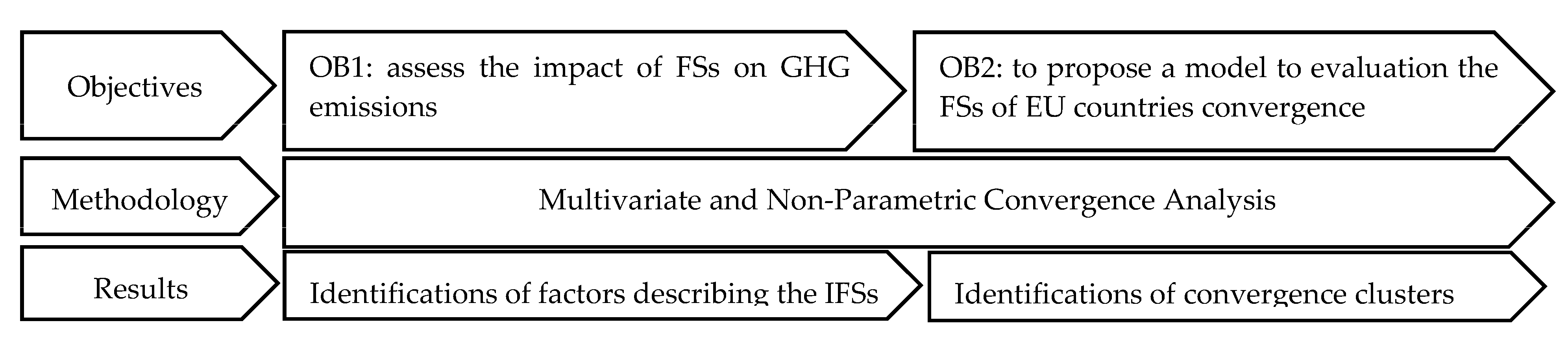
Figure 1 shows the methodology adopted to reach each objective reported in the introduction as well as the results obtained.

Agricultural land-use change was characterized by a data set collected from the latest statistical data available between 2009 and 2019 by the Food and Agriculture Organization of the United Nations (FAO) data sources [29,30]. All data for the initial year 2009 and the final year 2019 were considered. More details are presented in

Table 1. List of starting variables employed in the multivariate and non-parametric analyses.

N.	Item	Indicator	Element	Unit
1	Nutrient nitrogen N (total)	N	Use per area of cropland	kg/ha
2	Nutrient phosphate P2O5 (total)	P2O5	Use per area of cropland	kg/ha
3	Nutrient potash K2O (total)	K2O	Use per area of cropland	kg/ha
4	Pesticides	Pesticides	Use per area of cropland	kg/ha
5	Agricultural land	Agr.Land	Share in Land area	%
6	Arable land	Ar.Land	Share in Agricultural land	%
7	Land under permanent crops	LandUPC	Share in Agricultural land	%
8	Cropland	Cropland	Share in Land area	%
9	Land under perm. meadows and pastures	LandUPMP	Share in Land area	%
10	Forest land	F.Land	Share in Land area	%
11	Planted Forest	PlantedF.	Share in Forest land	%
12	Naturally regenerating forest	NRF	Share in Forest land	%
13	Agriculture area under organic agriculture	Agr.AUOA	Share in Agricultural land	%
14	Cattle	Cattle	Livestock units per agricultural land area	LSU/ha
15	Chickens	Chickens	Share in total livestock	LSU/ha
16	Pigs	Pigs	Livestock units per agricultural land area	LSU/ha
17	Sheep	Sheep	Livestock units per agricultural land area	LSU/ha
18	Cropland organic soils	CCO2	Emissions (C CO2)	kilotonnes
19	Cropland organic soils	CN2O	Emissions (CN2O)	kilotonnes
20	Grassland organic soils	GCO2	Emissions G(CO2)	kilotonnes
21	Grassland organic soils	GN2O	Emissions (GN2O)	kilotonnes
22	Enteric Fermentation	EFCH4	Emissions (EFCH4)	kilotonnes
23	Forest fires	FFCH4	Emissions (FFCH4)	kilotonnes
24	Forest fires	FFN2O	Emissions FF(N2O)	kilotonnes
25	Forestland	FLCO2	Emissions (FL CO2)	kilotonnes
26	Manure Management	MMCH4	Emissions (MMCH4)	kilotonnes
27	Manure Management	MMN2O	Emissions (MMN2O)	kilotonnes

Source: author elaboration of data from FAO, 2009 and 2019.

. Given the fact that IFSs are responsible for GHG emissions, this empirical study assesses the relationship between the use of pesticides, fertilizers, livestock raising, and changes in land use and GHG emissions. As is well known, CO₂ emissions are generated by the utilization of pollutants. However, as Aryal et al. [31] have argued, significant fertilizer use increases, above all, crop production. In this study, fertilizer consumption, expressed in kilograms per hectare (kg/ha) of arable land, indicates the quantity of plant nutrients utilized per unit of arable land. Fertilizer products include potash (K₂₀) and nitrogenous (N) and phosphate (P₂₀₅) fertilizers. As pointed out by Sharma et al. [32], the use of pesticides per area of cropland (kg/ha) is one of the essential measures of modern agricultural practices in protecting crops from different pests. Therefore, pesticide use in EU countries has led to a range of problems for agriculture, the environment, and human health [33,34]. Instead, the analysis of land cover changes from 2009 to 2019 is essential to highlight the dynamics of agricultural activities. For this purpose, nine indicators (from 5 to 13, Table 1) were selected related to the share for different purposes vis-a-vis the total land area. Furthermore, livestock influences the climate through land use change for feed production, animal production, and manure. Feed production and manure emit CO₂, N₂O, and CH₄, which consequently affects climate change [35]. Animal production increases CH₄ emissions. Several authors pointed out that the livestock sector is often associated with negative environmental impacts such as land degradation, air and water pollution, and biodiversity destruction [36,37,38,39]. Furthermore, enteric fermentation is the largest contributor to emissions from the sector.

2.2. Statistical Analysis

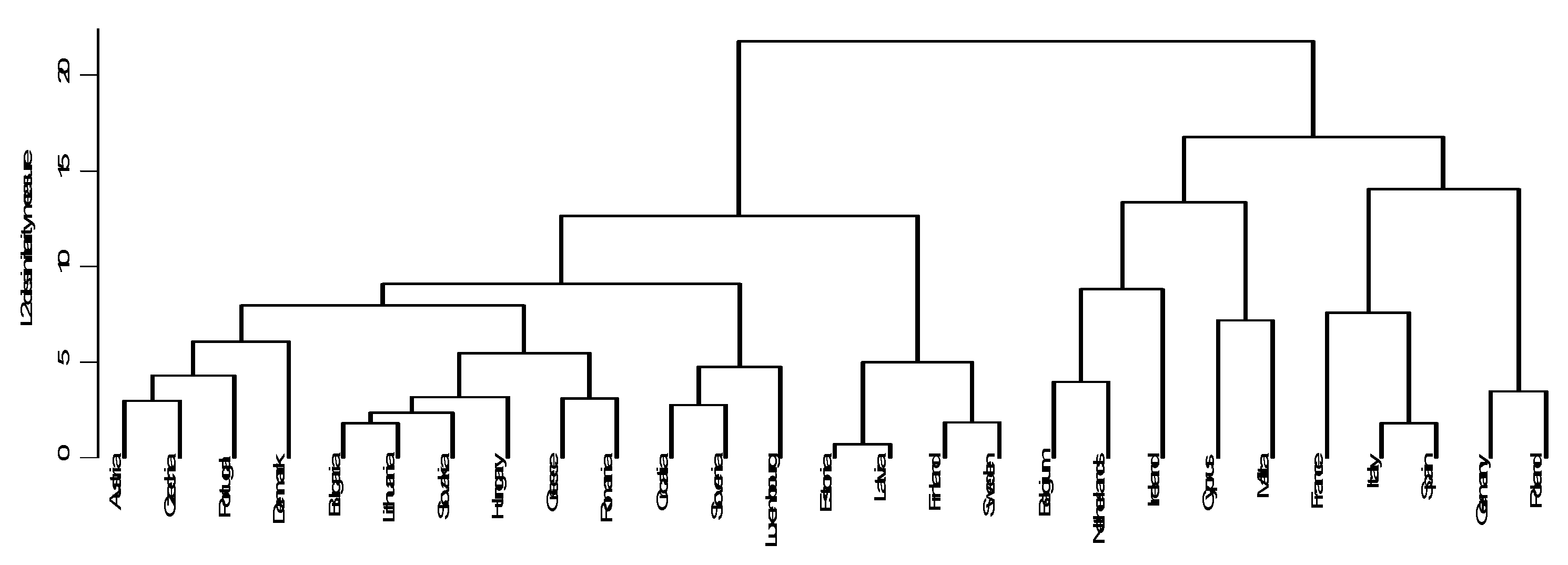
Multivariate and non-parametric convergence analyses were implemented to carry out quantitative measurements of the similarity levels and the degree of affinity among countries. According to the characteristics of 27 indicators related to the environmental aspects of growing and to the use of pesticides and fertilizers, especially in terms of their impact on GHG emissions, comparisons were made and various clusters were differentiated (Table 1). The results of numerical analysis can be clearly expressed by a dendrogram acquired from the hierarchical cluster analysis (HCA). These results were quite helpful for the objective analysis and provided a reasonable evaluation of the gaps between countries in relation to their agricultural production methods.

There are numerous kinds of clustering methods. In this study, the STATA programmer (Stata 12.32, software package created in 1985 by Stata Corp, College Station, TX, USA) was used. It utilizes two principal methods: one is the K-Means Cluster method and the other is the hierarchical Cluster (HC) method [40]. A comparative analysis of the dynamics and structure of the 27 Member States with different levels of intensification of agricultural productions was carried out with Ward’s method [41] of measuring squared Euclidean distance.

Data processing was performed in two successive phases: a core principal component analysis (PCA) and an HCA.

Firstly, to understand common patterns among countries, PCs were extracted. Prior communality estimates were set to one and components with an eigenvalue of less than one were dropped from the analysis. A varimax variable rotation was used to arrive at the PCs presented in Section 3. Significant loadings onto a PC were defined as those with a loading greater than 0.30 in absolute value. Once the analysis of “similarity” with the “mapping” of EU countries was carried out, the convergence hypothesis was tested utilizing variance testing in the 2009 and 2019 scenarios. The convergence process of utilized performance variables towards a more sustainable agricultural production was tested. With reference to the 27 Member States, based on two indicators, the standard deviation α and a synthetic index β were used [42,43,44]. The approach to the analysis of convergence presented in this paper is based on the conditioning scheme originally proposed by Quah [43].

The α was calculated as the difference between the average squared deviation in the levels of all indicators in the initial year (2009) and the final year (2019). If the value of the indicator increases over the ten-year period between 2009 and 2019, it undergoes a convergence process. Conversely, if it decreases, there is a divergence process.

In contrast, the synthetic indicator β, constructed as a ratio between the final value of the standard deviation and the initial value can assume higher, equal, or lower values than 1, depending on whether a divergence, stationary, or convergence process is in progress in relation to utilized performance variables. The discrepancy between divergence and convergence will then be based on the values read at the synthetic indicator β. The values assumed by the indices α and β can be accepted as weak convergence (or divergence) indices, as this is a convergence/divergence process conditioned by country choice and sustainability of agricultural production systems.

3. Results and Discussion

3.1. Changes in FSs Intensification between 2009 and 2019

Table 2. Descriptive statistics of EU countries.

Variable	2009					2019
	Mean	Std. Dev	Min	Max	CV	Mean	Std. Dev.	Min	Max	CV
N	83.46	48.72	30.97	211.34	0.58	95.72	43.86	48.62	217.19	0.46
P2O5	15.89	10.73	0.65	46.39	0.68	21.85	8.61	10.09	42.51	0.39
K2O	15.88	15.17	1.16	67.63	0.95	28.10	18.36	8.53	79.31	0.65
Pesticides	2.82	2.52	0.00	9.04	0.89	3.12	2.59	0.00	9.98	0.83
Agr.Land	42.07	16.96	7.53	66.68	0.40	41.22	15.86	7.38	65.67	0.38
Ar.Land	62.08	20.37	10.07	98.34	0.33	62.45	20.89	9.79	98.72	0.33
LandUPC	5.79	7.62	0.07	28.53	1.32	5.72	7.36	0.02	21.86	1.29
Cropland	27.24	13.34	6.46	60.92	0.49	26.98	13.01	6.25	60.48	0.48
LandUPMP	14.83	12.04	0.00	59.93	0.81	14.24	11.51	0.00	59.22	0.81
F.Land	34.29	17.23	1.09	73.26	0.50	34.85	17.16	1.44	73.73	0.49
PlantedF.	36.15	30.17	0.00	96.85	0.83	36.66	29.04	3.56	95.02	0.79
NRF	63.93	30.08	3.15	100.00	0.47	63.32	29.07	4.98	96.44	0.46
Agr.AUOA	5.22	4.27	0.24	18.56	0.82	9.33	6.27	0.29	25.34	0.67
Cattle	0.51	0.51	0.07	1.86	1.00	0.50	0.48	0.06	1.84	0.96
Chickens	0.12	0.23	0.01	1.16	1.96	7.30	8.45	0.00	25.67	1.16
Pigs	0.35	0.45	0.03	1.59	1.30	0.30	0.41	0.02	1.64	1.34
Sheep	0.04	0.05	0.00	0.24	1.26	0.03	0.04	0.00	0.14	1.13
CCO2	2229.70	3180.77	0.00	12,672.99	1.43	2253.62	3189.41	0.00	12,550.61	1.42
CN2O	1.35	2.13	0.00	8.69	1.58	1.37	2.14	0.00	8.61	1.57
GCO2	118.49	179.20	0.00	690.34	1.51	120.34	180.01	0.00	687.57	1.50
G N2O	1.08	1.99	0.00	7.46	1.84	1.11	2.01	0.00	7.59	1.81
EFCH4	251.67	345.33	1.60	1455.48	1.37	237.88	322.33	1.35	1333.70	1.36
FFCH4	0.06	0.11	0.00	0.51	2.08	0.09	0.21	0.00	0.94	2.33
FFN2O	0.00	0.01	0.00	0.05	2.52	0.01	0.02	0.00	0.09	2.30
FLCO2	−16,427.12	22,866.58	−84,614.57	−0.45	−1.39	−12,237.69	18,604.49	−67,236.84	0.00	−1.52
MMCH4	69.33	93.59	1.30	320.95	1.35	66.51	92.73	0.80	308.81	1.39
MMN2O	2.50	3.31	0.02	12.99	1.32	2.35	3.14	0.01	12.09	1.33

Source: author elaboration of data from FAO, 2009 and 2019.

provides descriptive statistics of the 27 indicators used in the analysis.

The average utilization of fertilizers from 2009 to 2019 increased. This may be due, in accordance with Chen et al. [5], to the fact that many farmers have applied excessive N fertilizers to realize high crop yields. As is well known, increased use of nutrient fertilizers such as N, P₂₀₅, K₂₀ and pesticides can increase nutrient contents in surface and groundwater; in surface water, this can lead to eutrophication from algal growth. Furthermore, the use of N fertilizers is an important driver of energy use and GHG emissions in EU countries [45].

From 2009 to 2019, the consumption of all chemical fertilizers per unit area of land (kg/ha) increased, and in particular, there was a rise in the utilization of N (Table 2). The range of pesticides between the minimum and the maximum values was the largest, and its coefficient of variation (CV), equal to 0.83 for 2009 and 0.89 for 2019, was also the highest of the four agrichemicals utilized in the analysis. This suggests that a number of EU countries are seeing major changes in their pesticide use and that FSs in these countries, in accordance with Tudi et al. [34], have become more intensive over the past ten years because of the urgency to improve food production. Indeed, as suggested by other authors [46], the increase in the use of pesticides is correlated to population growth and to climate change.

The CVs for the other three pollutants were between 89 and 124%. This means that human activities have a significant impact on the concentrations of most metal pollution in soils throughout the EU. The use of these agrochemicals may have resulted in undesirable concentrations of metals in the environment [32].

Another important indicator is land use change that can simultaneously cause both beneficial and harmful effects. Indeed, any change in land use has important consequences for many biological, chemical, and physical processes in soils and, consequently, the environment [47]. If, for instance, in accordance with Wang [48], arable land is converted to grass or forestry for sequestering purposes, this may require more intensive cultivation in other areas to compensate for yield losses (with possible GHG consequences) or else it may trigger land clearance in order to grow food elsewhere.

Nine types of land uses (agricultural land, arable land, land under permanent crops, cropland, land under permanent meadows and pastures, forestland, planted forest, naturally regenerating and agriculture areas under organic agriculture) were considered for this study of the EU. The mean concerning variation in the use of agricultural land indicates that in the period 2009–2019, there was a decrease in these indicators. Agriculture lands cover about 38.5% of the global total land area, which consists of 28.4% of arable land and 68.4% of permanent meadows and pasture.

The increasing demand for livestock products has significantly changed the natural landscape. The GHG emissions from animal husbandry and agricultural soils are the highest in countries with high animal densities, such as the Netherlands and Belgium [49]. Indeed, according to the national inventory of the Netherlands [20], agricultural activities emitted 506 Gg CH₄ and 22 Gg N₂O in the reference year 1990.

Pigs and poultry require even less land and produce fewer emissions than ruminants since their feed conversion efficiency is greater and CH₄ is less of an issue. Recent years have seen rapid growth in the production and consumption of pig and poultry products. This trend is anticipated to continue and is considered positive from a GHG perspective [29,50].

Intensive rearing systems are also associated with other environmental problems including soil and water pollution [51]. An EU country’s off-site problem is the production of GHG gases by IFS, including the conversion of forest to farmland.

The use of N fertilizers induces CO₂ emissions by process and by combustion from the production of ammonia, CO₂ emissions by combustion from the synthesis of N fertilizers from ammonia, and N₂O emissions from denitrification of nitrogen inputs. This is a result of reducing the amount of N applied per hectare, which has a significant effect on N₂O emissions and reducing the number of dairy cattle and sheep, which have an impact on CH₄ emissions. However, higher emissions from enteric fermentation varied across countries [52].

With respect to other agricultural land uses, grassland is one of the dominant forms of land use, covering 34% of the EU’s agricultural area [53], and requires careful management attention [54] because any change in grasslands’ ability to deliver ecosystem services will have significant societal impacts. However, the effect of indicators on grasslands and farms [55] is different, and in some cases, as in Italy, this has resulted in less intensive levels than arable systems [56].

3.2. Discussion of Results from Multivariate Analysis

As mentioned above, a multivariate analysis was performed in two successive phases: the PCA and the HCA.

The analysis of the main PCs highlighted the differences in the variables of the agricultural system in the 27 countries of the EU and led to the identification of 8 main PCs for both 2009 and 2019. Overall, these 8 main PCs accounted for 91% of the total variability for 2009 and 90% for 2019 with a very low information loss of 9% and 10% respectively (

Table 3. Variance explained by the main components.

PCs	2009		2019
	Proportion	Cumulative	Proportion	Cumulative
PC1	0.24	0.24	0.24	0.24
PC2	0.18	0.42	0.18	0.42
PC3	0.15	0.57	0.16	0.58
PC4	0.10	0.67	0.10	0.67
PC5	0.09	0.76	0.08	0.75
PC6	0.06	0.82	0.06	0.81
PC7	0.05	0.87	0.05	0.86
PC8	0.04	0.91	0.04	0.90

Source: author elaboration of data from FAO, 2009 and 2019.

).

PC1 explained 24% of the variance in the data while both PCs 1 and 2 explain 42% of the variance.

Both for 2009 and for 2019, agricultural system variables that most influence the first major PCs—that alone account for 42% of variance—can be characterized as follows:

PC1: indicates the countries both for 2009 and for 2019 (Germany, France, Ireland, Poland, Netherlands) with a high intensity of GHG emissions from grassland, enteric fermentation and manure management;

PC2: explains two different phenomena for 2009 and for 2019. The first year considered indicates the countries (Netherlands, Ireland, Belgium, Cyprus, Malta, Luxembourg) with intensity in cattle livestock, and for 2019, countries (France, Poland, Germany, Sweden, Finland) with a high emission of CCO₂ from croplands.

Table 4. FSs variables characterising the first two main components.

Variables 2009				Variables 2019
With Negative Sign		With Positive Sign		With Negative Sign		With Positive Sign
PC1				PC1
P2O5	−0.01	N	0.16	Agr.Land	−0.12	N	0.14
Ar.Land	−0.07	K2O	0.15	LandUPC	−0.04	P2O5	0.06
LandUPC	−0.09	Pesticides	0.13	F.Land	−0.19	K2O	0.22
F.Land	−0.13	Agr.Land	0.23	PlantedF.	0.20	Pesticides	0.19
NRF	−0.18	Cropland	0.13	NRF	−0.20	Agr.Land	0.24
Agr.AUOA	−0.10	LandUPMP	0.18	Agr.AUOA	−0.17	Cropland	0.10
Chickens	−0.04	PlantedF.	0.18	Chickens	−0.10	LandUPMP	0.22
Sheep	−0.07	Cattle	0.15	FLCO2	−0.17	Cattle	0.21
FLCO2	−0.19	Pigs	0.03			Pigs	0.13
		CCO2	0.21			Sheep	0.04
		CN2O	0.19			CCO2	0.14
		GCO2	0.32			CN2O	0.12
		GN2O	0.28			GCO2	0.31
		EFCH4	0.34			GN2O	0.27
		FFCH4	0.17			EFCH4	0.31
		FFN2O	0.17			FFCH4	0.13
		MMCH4	0.32			FFN2O	0.13
						MMCH4	0.29
						MMN2O	0.32
With negative sign		With positive sign		With negative sign		With positive sign
PC2				PC2
Ar.Land	−0.20	N	0.24	N	−0.21	Ar.Land	0.20
Cropland	−0.02	P2O5	0.10	P2O5	−0.04	F.Land	0.22
F.Land	−0.29	K2O	0.21	K2O	−0.19	NRF	0.14
NRF	−0.16	Pesticides	0.27	Pesticides	−0.22	Agr.AUOA	0.12
Agr.AUOA	−0.16	Agr.Land	0.13	Agr.Land	−0.09	Chickens	0.15
CCO2	−0.25	LandUPC	0.10	LandUPC	−0.07	CCO2	0.32
CN2O	−0.24	LandUPMP	0.20	LandUPMP	−0.20	CN2O	0.29
GN2O	−0.02	PlantedF.	0.16	PlantedF.	−0.14	GCO2	0.11
EFCH4	−0.11	Cattle	0.32	Cattle	−0.29	GN2O	0.08
FFCH4	−0.16	Chickens	0.20	Pigs	−0.23	EFCH4	0.21
FFN2O	−0.15	Pigs	0.28	Sheep	−0.13	FFCH4	0.17
MMCH4	−0.09	Sheep	0.19	FFN2O	−0.34	FFN2O	0.17
MMN2O	−0.11	GCO2	0.00			FLCO2	0.17
		FFN2O	0.30			MMCH4	0.21
						MMN2O

Source: author elaboration of data from FAO, 2009 and 2019.

illustrates the main phenomena synthesized by the two PCs.

In particular, EU countries present negative values for the incidence of agricultural land use vis-a-vis the land area, for the presence of the forestland and, for the incidence of chickens and sheep per hectare in relation to the total for livestock. Whereas there were positive values, above all, for GHG emissions. The analysis of the key factors demonstrated a high level of “heterogeneity” among EU countries, which is in line with Pawlak et al. [57].

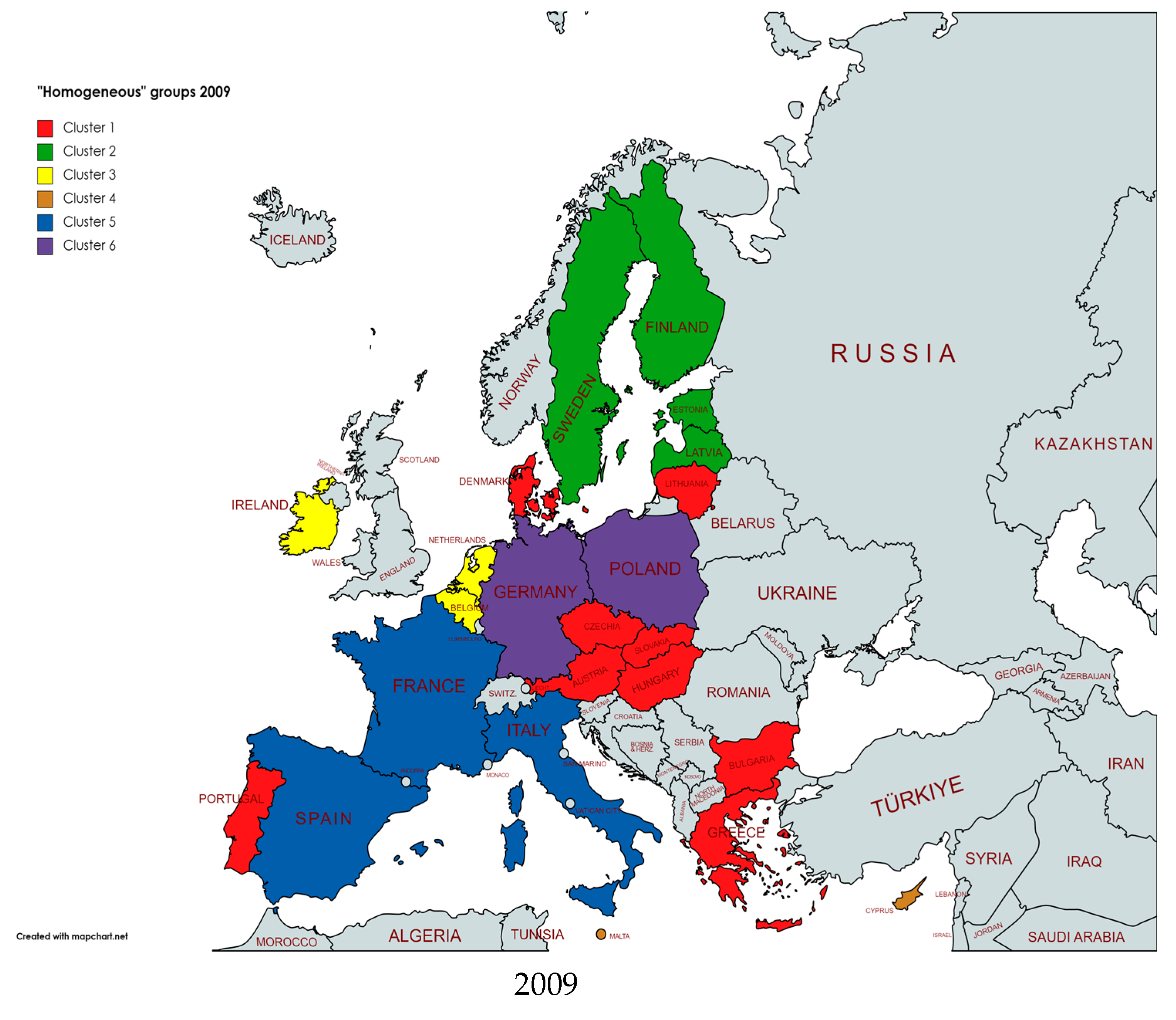
Furthermore, the statistical analysis carried out on the main PCs of the 2009 and 2019 agricultural systems allowed the 27 Member States to be grouped into 6 significant clusters or “homogeneous” groups.

For 2009, the division into clusters (Figure 2 and Figure 3), using the complete linkage method, is as follows:

Cluster 1 includes 13 countries (which represent 48% of the total), located in northern and central Europe. The main characteristic of this first and largest group is the high reduction in the emission of CO₂ from forestland. Slovenia and Slovakia show the highest reduction, −11,895.5 and −8863.15 kilotonnes, respectively.

Cluster 2 consists of four countries, showing a dynamic in the use of pollutants. On average, the countries of this group, especially Finland and Sweden, highlight a high emission of CCO₂ from croplands. On average, the countries of this group, especially Finland and Sweden, highlight a high emission of CCO₂ from croplands.

Cluster 3 includes the countries that show the highest average use per area of cropland (kg/ha) of all pollutants and pesticides, especially the use of K_2O. On average, the countries of this group, in particular Ireland, show a high share of land under permanent crops in relation to the total land area. Furthermore, the countries of this group show a high incidence of cattle units per agricultural land area (LSU/ha). As is well documented, the latter are the main source of CH₄ emissions compared to other ruminants, such as sheep.

In Cluster 4, there are only two countries: Cyprus and Malta. For this group, almost all the variables considered have below EU average values. Thus, this group is characterized by an absence of emissions from crops and from grasslands.

Cluster 5 groups together three countries (France, Italy and Spain) and is characterized, with respect to other clusters, by the low use of pollutants, especially N, and for high emissions of manure, measured in kilotonnes.

Cluster 6 consists, like Group 4, of only two countries (Germany and Poland) that, on average, in respect to the other five clusters, highlight the lowest use of pesticides per area of cropland (236 kg for ha).

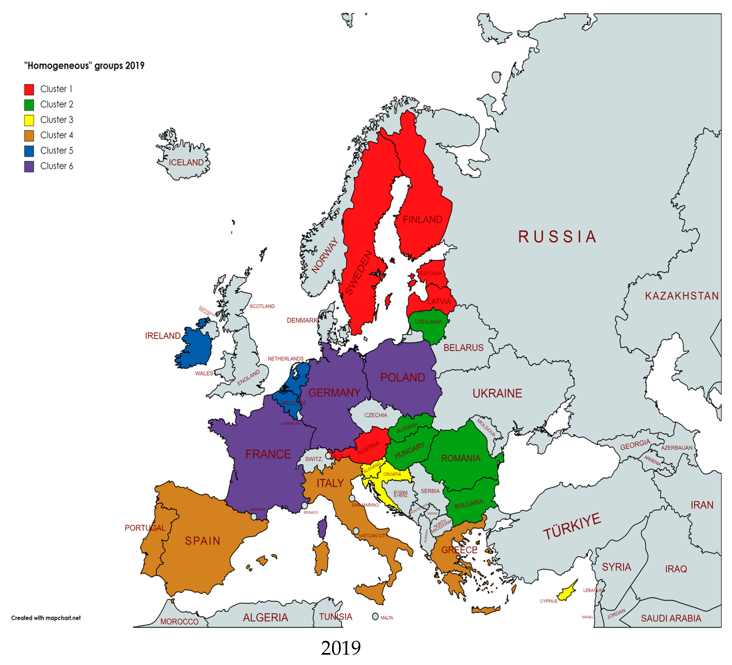
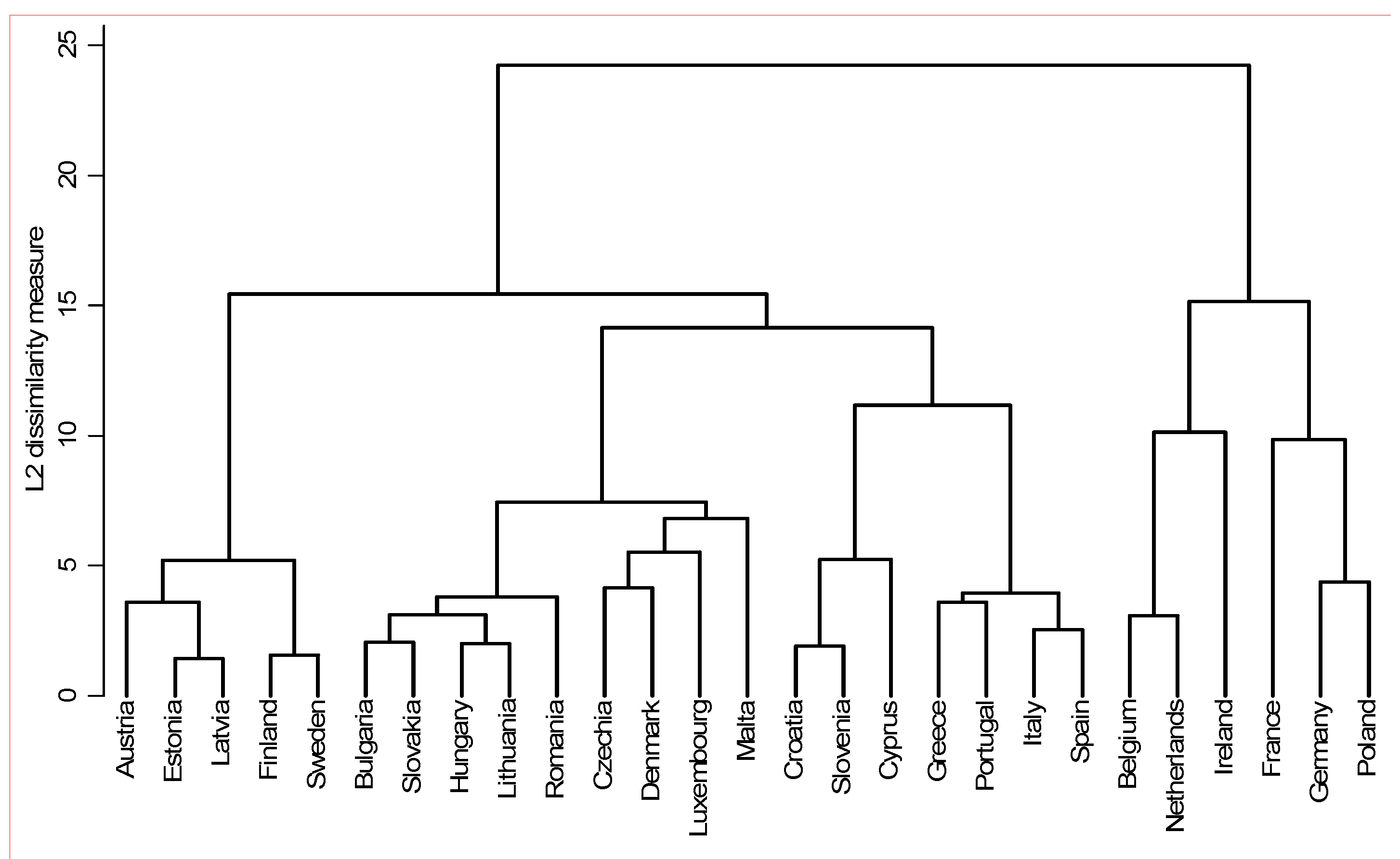
The 2019 cluster analysis conducted on the main PCs also generated six “homogeneous” groups of countries (Figure 3 and Figure 4).

Cluster 1 includes five countries (Austria, Estonia, Finland, Latvia, and Sweden) that, on average, show the highest incidence of forest land in the land area (60% vs. circa 35% of the global mean) and the highest incidence of organic agriculture in an agricultural area (19.27% vs. 9.33 of the global mean).

Cluster 2 is the largest, with nine countries (33% of the total EU countries), that, on average, present the highest share of agricultural land, arable land, and cropland in relation to the total land area.

Cluster 3 includes three countries, and is characterized by a high incidence of both the use of nutrient phosphate per area of cropland (38.48 kg/ha vs. 21.85 of the global mean) and of naturally regenerating forest on forest land (91.26 vs. 63.32 of the global mean).

Cluster 4 contains four EU countries with the highest presence of land under permanent meadows and pastures in relation to the total land area (19.22% vs. 5.72 of the global mean). Furthermore, this area has the highest share of sheep in relation to the total livestock area, suggesting a transition of these countries towards an intensification of agricultural activities.

Cluster 5 includes three EU countries with a strong presence of intensive agricultural activities, especially in terms of the use of both N per area of cropland (kg/ha) and pesticides, and in the presence of cattle.

Cluster 6, like Cluster 5, has only three EU countries that are the most responsible for crop, grassland, and livestock emissions with respect to the other five groups.

3.3. Discussion of Results from Non-Parametric Convergence Analysis

The values assumed by the indices α and β (

Table 5. Standard deviation and synthetic index.

Variables	Stand Dev 2009	Stand Dev 2019	α	Convergence/Divergence	β	Convergence/Divergence
N	83.46	43.86	−39.6	Divergence	0.53	Convergence
P2O5	15.89	8.61	−7.28	Divergence	0.54	Convergence
K2O	15.88	18.36	2.48	Convergence	1.16	Divergence
Pesticides	2.82	2.59	−0.23	Divergence	0.92	Convergence
Agr.Land	42.07	15.86	−26.21	Divergence	0.38	Convergence
Ar.Land	62.08	20.89	−41.19	Divergence	0.34	Convergence
LandUPC	5.79	7.36	1.57	Convergence	1.27	Divergence
Cropland	27.24	13.02	−14.22	Divergence	0.48	Convergence
LandUPMP	14.83	11.51	−3.32	Divergence	0.78	Convergence
F.Land	34.29	17.16	−17.13	Divergence	0.5	Convergence
PlantedF.	36.15	29.04	−7.11	Divergence	0.8	Convergence
NRF	63.93	29.07	−34.86	Divergence	0.45	Convergence
Agr.AUOA	5.22	6.27	1.05	Convergence	1.2	Divergence
Cattle	0.51	0.48	−0.03	Divergence	0.94	Convergence
Chickens	0.12	8.45	8.33	Convergence	70.42	Divergence
Pigs	0.35	0.41	0.06	Convergence	1.17	Divergence
Sheep	0.04	0.04	0,00	Convergence	1,00	Convergence
CCO2	2229.7	3189.41	959.71	Convergence	1.43	Divergence
CN2O	1.35	2.14	0.79	Convergence	1.59	Divergence
GCO2	118.49	180.01	61.52	Convergence	1.52	Divergence
GN2O	1.08	2.01	0.93	Convergence	1.86	Divergence
EFCH4	251.67	322.33	70.66	Convergence	1.28	Divergence
FFCH4	0.06	0.21	0.15	Convergence	3.5	Divergence
FFN2O	0,00	0.02	0.02	Convergence	0,00	Divergence
FLCO2	−16,427.12	18,604.49	35,031.61	Convergence	−1.13	Divergence
MMCH4	69.33	92.74	23.41	Convergence	1.34	Divergence
MMN2O	2.5	3.14	0.64	Convergence	1.26	Divergence

Source: Author elaboration of data from FAO, 2009 and 2019.

) can be accepted as weak convergence (or divergence) indices, as this is a convergence/divergence process conditioned by country choice and agricultural system variables.

Table 5 also shows that the value of α 1 (α 1, 2019–α 1, 2009) decreased mainly for the following agricultural systems variables: the share of the arable land; for the kg of N used per area of cropland; and the naturally regenerating forest (NRF). The standard deviation values α 1, 2009 and α 1, 2019 show an increase in the dispersion of variables examined around the mean quadratic average values over time, with a tendency towards divergence among countries with a high percentage of arable and agricultural land and those characterized by high livestock intensity.

Conversely, the synthetic index β highlights a divergence process for most variables and for all countries but shows a greater tendency for eco-friendlier countries to move away from those that continue to have IFSs. In accordance with Giller et al. [58], this process was also influenced by the need to reform “conventional” agriculture according to the principles of agroecology, organic agriculture, and (increasingly) regenerative agriculture.

Table 6. Transition matrix.

	Cluster 2019							Tot
	1		2	3	4	5	6
Cluster 2009	1	A	BG, CZ, DK, H, LT, L, M, RO, SK	HR	GR			12
	2	EW, FIN, LV, S		SLO				5
	3					B, IRL, NL		3
	4		M	CY				2
	5				I, E		F	3
	6						D, PL	2

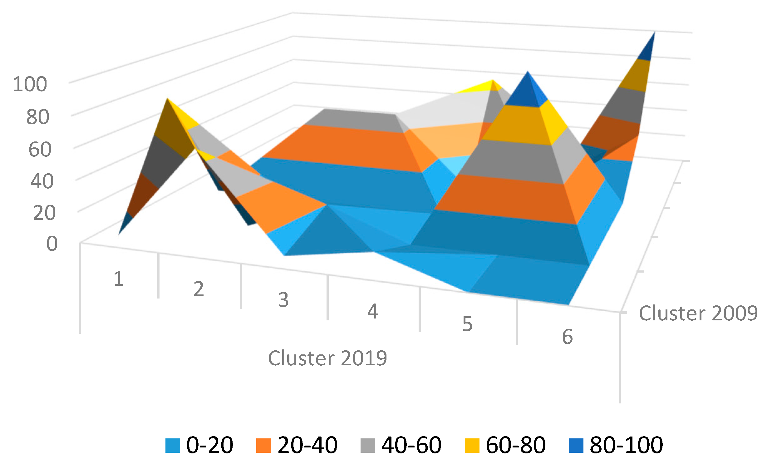
Source: Author elaboration of data from FAO, 2009–2019.

shows that most EU countries have not remained in the same groups. The percentage value that appears in the transition Markoviana matrix [43] indicates the number of times a country that belonged to one of the initial groups in 2009 passed into the same group in 2019. The most obvious element with reference to the transition matrix (TM) is that many countries have moved from their original group. Indeed, in the first row of the TM, for example, only Austria (A) of the twelve EU countries that in 2009 were in Cluster 1 remained in the same cluster in 2019. Seventy-five percent (Bulgaria, Czech Republic, Denmark, Hungary, Lithuania, Luxemburg, Malta, Romania and Slovakia) passed to Cluster 2, and just two countries (Croatia and Greece) passed to Clusters 3 and 4, respectively. The second line shows that 80% (Estonia, Finland, Latvia and Sweden) of the five countries that in 2009 belonged to Group 2 migrated to Group 1; the remaining 20% (Slovenia) moved to Group 3. The figures in the third line indicate that the three countries (Belgium, Ireland and the Netherlands) that belonged to Group 1 in 2009 had moved to Group 3 by 2019. The fourth line shows that the two countries (Cyprus and Malta) that in 2009 were in Cluster 4 passed to Clusters 2 and 3, respectively. The fifth line shows that the three countries (France, Italy and Spain) that belonged in 2009 to Group 5 had moved to Group 4 (Italy and Spain) and 6 (France), respectively. Lastly, the sixth line shows that the two countries (Germany and Poland) that belonged to Group 6 in 2009 had remained in Group 6 by 2019. A process of divergence has therefore occurred. The TM allowed a three-dimensional graph to be drawn (Figure 5).

The main conclusion from this part of the analysis, in line with the literature on growth and convergence [59], confirms that, from 2009 to 2019, the β convergence hypothesis interested, above all, countries with initially high levels of IFSs (Belgium, Hungary, Luxemburg, Romania). These countries tend to differ over time from those that have recently adopted an intensive agricultural system with high GHG emissions (Estonia, Finland, Latvia, and Sweden). These results can be verified by simply observing the data on the trends in EU countries’ FSs (Table 3). It is possible, in accordance with Schmalensee et al. [60], that high-income countries have continued to reduce their CHG emissions over the 2009–2019 period. Conversely, others in the same area, such as Sweden and Finland, have increased these emissions in the same period. Moreover, some Eastern European countries, such as Bulgaria, Czechia, Hungary, Poland, and Slovakia, have reduced GHG emissions even more than the richest EU countries.

4. Conclusions

In this study, some evidence concerning the magnitude, direction, and geographic distribution of fertilizers, pesticides, land-use trends, livestock raising, and GHG emissions are provided. For this purpose, the investigation was conducted on two different stages in order to highlight similarities/dissimilarities among the 27 countries in the study and to understand if they are converging towards a more sustainable agricultural system.

In the first stage, the PCA and subsequent CA have classified the Member States into six “homogeneous” FSs, which differ considerably in terms of the the emissions of CO₂, N₂O, and CH₄ from cropland, grassland, forest, enteric fermentation, and manure management. Despite these differences, there is great “homogeneity” among the same countries regarding the share of arable land set aside for arable farming and the share of the land area used for agricultural land. This classification can play a fundamental role in the implementation of a Common Agricultural Policy (CAP) because the identification of areas with similar characteristics can be the target of specific actions. This is because the post-2020 discussion on the CAP has increased the discretionary power of Member States. in selecting and designing their specific agricultural measures within a common EU framework. This new classification can also be used to identify areas for investigation in comparative studies or field surveys, as a basis for selecting case study areas or to compare the EU countries with similar features or needs.

Furthermore, data presented here can be used to complement the information provided by previous classification systems [27,28,61], depending on the specific needs of the users such as studying possible relationships between agriculture intensity and other relevant ecological or socio-economic geospatial information.

In the second stage, the results of a non-parametric convergence analysis made it possible to give a clearer picture of the dynamics of the convergence process. In summary, these findings are consistent with earlier studies that analysed the convergence of GHG emissions in EU countries using approximate indicators. Indeed, as noted by some authors [19,20,62], increased food consumption has contributed to a convergence in pollutant use and to an increase in agricultural production across EU countries. However, the analysis shows that during the entire study period, the convergence hypothesis has interested mainly countries with initially high levels of intensive farming (Belgium, Hungary, Luxemburg, and Romania) that tend to differ over time from those that have recently adopted an intensive agricultural system with high GHG emissions (Estonia, Finland, Latvia, and Sweden).

From a dynamic point of view, the results point to the existence of six convergence clusters.

The paper contributes to the existing literature in two ways:

(i) To my knowledge, this is the first study in which a broad range of indicators to estimate the contribution of fertilizers, pesticides, land-use trends, and livestock to GHG emissions has been considered in a comparable level of detail;

(ii) Secondly, the methodological approach that was used to measure convergence allows the countries to be classified in a flexible way inside convergence clusters. This approach is especially suited for environmental variables where the classical concepts of convergence (conditional) may be too rigid to be fulfilled. Moreover, this methodology allows the dynamics of the convergence process to be measured.

Finally, a new and more accurate classification of EU countries in “homogeneous” territorial agricultural systems is essential to improve the comparability of countries for the development of the environmental programmes of the CAP for the period 2023–2027.

References

- The Intergovernmental Panel on Climate Change (IPCC). Climate Change and Land. Special Report on Climate Change, Desertification, Land Degradation, Sustainable Land Management, Food Security, and Greenhouse Gas Fluxes in Terrestrial Ecosystems. Available online: https://www.ipcc.ch/srccl/ (accessed on 12 October 2022).
- Meinshausen, M.; Meinshausen, N.; Hare, W.; Raper, S.C.B.; Frieler, K.; Knutti, R.; Frame, D.J.; Allen, M.R. Greenhouse-gas emission targets for limiting global warming to 2 °C. Nature 2009, 458, 1158–1162. [Google Scholar] [CrossRef] [PubMed]
- Kanter, D.R.; Musumba, M.; Wood, S.L.; Palm, C.; Antle, J.; Balvanera, P.; Dale, V.H.; Havlik, P.; Kline, K.L.; Scholes, R.J.; et al. Evaluating agricultural trade-offs in the age of sustainable development. Agric. Syst. 2018, 163, 73–88. [Google Scholar] [CrossRef]
- Luo, Q.; Gong, J.; Zhai, Z.; Pan, Y.; Liu, M.; Xu, S.; Wang, Y.; Yang, L.; Taoge-Tao, B. The responses of soil respiration to nitrogen addition in a temperate grassland in northern china. Sci. Total Environ. 2016, 569, 1466–1477. [Google Scholar] [CrossRef] [PubMed]
- Chen, Y.H.; Wen, X.W.; Wang, B.; Nie, P.Y. Agricultural pollution and regulation: How to subsidize agriculture? J. Clean. Prod. 2017, 164, 258–264. [Google Scholar] [CrossRef]
- Jabbar, F.K.; Grote, K. Statistical assessment of nonpoint source pollution in agricultural watersheds in the Lower Grand River watershed, MO, USA. Environ. Sci. Pollut. Res. 2019, 26, 1487–1506. [Google Scholar] [CrossRef]
- Overmars, K.P.; Schulp, C.J.E.; Alkemade, R.; Verburg, P.H.; Temme, A.J.A.M.; Omtzigt, N.; Schaminée, J.H.J. Developing a methodology for a species-based and spatially explicit indicator for biodiversity on agri-cultural land in the EU. Ecol. Indic. 2014, 37, 186–198. [Google Scholar] [CrossRef]
- Cruzeiro, C.; Pardal, M.A.; Rocha, E.; Rocha, M.J. Occurrence and seasonal loads of pesticides in surface water and suspended particulate matter from a wetland of worldwide interest—The Ria Formosa Lagoon, Portugal. Environ. Monit. Assess. 2015, 187, 669. [Google Scholar] [CrossRef]
- Jepson, P.C.; Guzy, M.; Blaustein, K.; Sow, M.; Sarr, M.; Mineau, P.; Kegley, S. Measuring pesticide ecological and health risks in West African agriculture to establish an enabling environment for sustainable intensification. Philos. Trans. Royal Soc. B Biol. Sci. 2014, 369, 20130491. [Google Scholar] [CrossRef]
- Kuemmerle, T.; Erb, K.; Meyfroidt, P.; Müller, D.; Verburg, P.H.; Estel, S.; Haberl, H.; Hostert, P.; Jepsen, M.R.; Kastner, T.; et al. Challenges and opportunities in mapping land use intensity globally. Curr. Opin. Environ. Sustain. 2013, 5, 484–493. [Google Scholar] [CrossRef]
- Niedertscheider, M.; Erb, K. Land system change in Italy from 1884 to 2007: Analysing the North-South divergence on the basis of an integrated indicator framework. Land Use Policy 2014, 39, 366–375. [Google Scholar] [CrossRef]
- Schneider, U.A.; Havlík, P.; Schmid, E.; Valin, H.; Mosnier, A.; Obersteiner, M.; Böttcher, H.; Skalský, R.; Balkovi, J.; Sauer, T.; et al. Impacts of population growth, economic development, and technical change on global food production and consumption. Agric. Syst. 2011, 104, 204–215. [Google Scholar] [CrossRef]
- Tuck, S.L.; Winqvist, C.; Mota, F.; Ahnström, J.; Turnbull, L.A.; Bengtsson, J. Land-use intensity and the effects of organic farming on biodiversity: A hierarchical meta-analysis. J. Appl. Ecol. 2014, 51, 746–755. [Google Scholar] [CrossRef]
- Lambin, E.F.; Rounsevell, M.D.A.; Geist, H.J. Are agricultural land-use models able to predict changes in land-use intensity? Agric. Ecosys. Environ. 2000, 82, 321–331. [Google Scholar] [CrossRef]
- Shriar, A.J. Determinants of agricultural intensity index “scores” in a frontier region: An analysis of data from northern Guatemala. Agric. Hum. Val. 2005, 22, 395–410. [Google Scholar] [CrossRef]
- Allan, E.; Bossdorf, O.; Dormann, C.F.; Prati, D.; Gossner, M.M.; Tscharntke, T.; Blüthgen, N.; Bellach, M.; Birkhofer, K.; Boch, S.; et al. Interannual variation in land-use intensity enhances grassland multidiversity. Proc. Natl. Acad. Sci. USA 2014, 111, 308–313. [Google Scholar] [CrossRef]
- Erb, K.H.; Haberl, H.; Jepsen, M.R.; Kuemmerle, T.; Lindner, M.; Müller, D.; Verburg, P.H.; Reenberg, A. A conceptual framework for analysing and measuring land-use intensity. Curr. Opin. Environ. Sustain. 2013, 5, 464–470. [Google Scholar] [CrossRef]
- Ewert, F.; Rounsevell, M.D.A.; Reginster, I.; Metzger, M.J.; Leemans, R. Future scenarios of European agricultural land use I. Estimating changes in crop productivity. Agric. Ecosyst. Environ. 2005, 107, 101–116. [Google Scholar] [CrossRef]
- Foley, J.A. Global consequences of land use. Science 2005, 309, 570–5744. [Google Scholar] [CrossRef]
- Klein Goldewijk, K.; Ramankutty, N. Land cover change over the last three centuries due to human activities: The availability of new global data sets. GeoJournal 2004, 61, 335–344. [Google Scholar] [CrossRef]
- Rounsevell, M.D.; Annetts, J.; Audsley, E.; Mayr, T.; Reginster, I. Modelling the spatial distribution of agricultural land use at the regional scale. Agric. Ecosyst. Environ. 2003, 95, 465–479. [Google Scholar] [CrossRef]
- Rounsevell, M.D.A.; Berry, P.M.; Harrison, P.A. Future environmental change impacts on rural land use and biodiversity: A synthesis of the ACCELERATES project. Environ. Sci. Policy. 2006, 9, 93–100. [Google Scholar] [CrossRef]
- Rounsevell, M.D.; Pedroli, B.; Erb, K.H.; Gramberger, M.; Busck, A.G.; Haberl, H.; Kristensen, S.; Kuemmerle, T.; Lavorel, S.; Linder, M.; et al. Challenges for land system science. Land Use Policy 2012, 29, 899–910. [Google Scholar] [CrossRef]
- Temme, A.J.A.M.; Verburg, P.H. Mapping and modelling of changes in agricultural intensity in Europe. Agric. Ecosyst. Environmen. 2010, 140, 46–56. [Google Scholar] [CrossRef]
- Hansen, J.; Sato, M.K.I.; Ruedy, R.; Nazarenko, L.; Lacis, A.; Schmidt, G.A.; Russell, G.; Aleinov, I.; Bauer, M.; Bauer, S.; et al. Efficacy of climate forcings. J. Geophys. Res. Atmos. 2005, 110. [Google Scholar] [CrossRef]
- Huston, M.A. The three phases of land-use change: Implications for biodiversity. Ecol. Appl. 2005, 15, 1864–1878. [Google Scholar] [CrossRef]
- Fanelli, R.M. The (un)sustainability of the land use practices and agricultural production in EU countries. Int. J. Environ. Stud. 2019, 76, 273–294. [Google Scholar] [CrossRef]
- Fanelli, R.M. The Spatial and Temporal Variability of the Effects of Agricultural Practices on the Environment. Environments 2020, 7, 33. [Google Scholar] [CrossRef]
- Food and Agriculture Organization (FAO). The State of Food and Agriculture 2009: Livestock in the Balance. Available online: https://www.fao.org/3/i0680e/i0680e.pdfRome (accessed on 12 October 2022).
- Food and Agriculture Organization (FAO). Food and Agriculture Data. Available online: https://www.fao.org/faostat/en/#home (accessed on 28 October 2022).
- Aryal, J.P.; Sapkota, T.B.; Krupnik, T.J.; Rahut, D.B.; Jat, M.L.; Stirling, C.M. Factors affecting farmers’ use of organic and inorganic fertilizers in South Asia. Environ. Sci. Pollut. Res. Int. 2021, 28, 51480–51496. [Google Scholar] [CrossRef]
- Sharma, A.; Kumar, V.; Shahzad, B.; Tanveer, M.; Sidhu, G.P.S.; Handa, N.; Kohli, S.K.; Yadav, P.; Bali, A.S.; Parihar, R.D.; et al. Worldwide pesticide usage and its impacts on ecosystem. SN Appl. Sci. 2019, 1, 1446. [Google Scholar] [CrossRef]
- Tegtmeier, E.M.; Duffy, M.D. External costs of agricultural production in the United States. Int. J. Agric. Sustain. 2004, 2, 1–20. [Google Scholar] [CrossRef]
- Tudi, M.; Daniel Ruan, H.; Wang, L.; Lyu, J.; Sadler, R.; Connell, D.; Chu, C.; Phung, D.T. Agriculture development, pesticide application and its impact on the environment. Int. J. Environ. Res. Public Health 2021, 18, 1112. [Google Scholar] [CrossRef] [PubMed]
- Grossi, G.; Goglio, P.; Vitali, A.; Williams, A.G. Livestock and climate change: Impact of livestock on climate and mitigation strategies. Anim. Front. 2019, 9, 69–76. [Google Scholar] [CrossRef] [PubMed]
- Bellarby, J.; Tirado, R.; Leip, A.; Weiss, F.; Lesschen, J.P.; Smith, P. Livestock greenhouse gas emissions and mitigation potential in Europe. Glob. Change Biol. 2013, 19, 3–18. [Google Scholar] [CrossRef] [PubMed]
- Reynolds, C.; Crompton, L.; Mills, J. Livestock and climate change impacts in the developing world. Outlook Agric. 2010, 39, 245–248. [Google Scholar] [CrossRef]
- Steinfeld, H.; Wassenaar, T.; Jutzi, S. Livestock production systems in developing countries: Status, drivers, trends. Rev. Sci. Techique 2006, 25, 505–516. [Google Scholar] [CrossRef]
- Thornton, P.K.; Gerber, P.J. Climate change and the growth of the livestock sector in developing countries. Mitig. Adapt. Strateg. Glob. Change 2010, 15, 169–184. [Google Scholar] [CrossRef]
- Zhang, T. Stata Statistic Analysis and Industry Application Cases; Tsinghua University Press: Beijing, China, 2014. [Google Scholar]
- Ward, J.H. Hierarchical grouping to optimize an objective function. J. Am. Stat. Assoc. 1963, 58, 236–244. [Google Scholar] [CrossRef]
- Boggio, L.; Seravalli, G. Sviluppo e Crescita Economica; McGrawHill Libri Italia srl.: Milano, Italy, 1999. [Google Scholar]
- Quah, D.T. Empirics for growth and distribution: Stratification, polarization, and convergence clubs. J. Econ. Growth 1997, 2, 27–59. [Google Scholar] [CrossRef]
- Sala-i-Martin, X.X. The classical approach to convergence analysis. Econ. J. 1996, 106, 1019–1036. [Google Scholar] [CrossRef]
- Menegat, S.; Ledo, A.; Tirado, R. Greenhouse gas emissions from global production and use of nitrogen synthetic fertilisers in agriculture. Sci. Rep. 2022, 12, 14490. [Google Scholar] [CrossRef]
- Tirado, M.C.; Clarke, R.; Jaykus, L.A.; McQuatters-Gollop, A.; Frank, J.M. Climate change and food safety: A review. Food Res. Int. 2010, 43, 1745–1765. [Google Scholar] [CrossRef]
- Borrelli, P.; Robinson, D.A.; Panagos, P.; Lugato, E.; Yang, J.E.; Alewell, C.; Wuepper, D.; Montanarella, L.; Ballabio, C. Land use and climate change impacts on global soil erosion by water (2015–2070). Proc. Natl. Acad. Sci. USA 2020, 117, 21994–22001. [Google Scholar] [CrossRef]
- Wang, X. Managing Land Carrying Capacity: Key to Achieving Sustainable Production Systems for Food Security. Land 2022, 11, 484. [Google Scholar] [CrossRef]
- Freibauer, A. Regionalised inventory of biogenic greenhouse gas emissions from European agriculture. Eur. J. Agron. 2003, 19, 135–160. [Google Scholar] [CrossRef]
- Department for Environment, Food & Rural Affairs (Defra). Food 2030. Department for the Environment, Food and Rural Affairs, UK. Available online: https://www.gov.uk/government/organisations/department-for-environment-food-rural-affairs (accessed on 9 September 2022).
- Food and Agriculture Organization (FAO). Livestock’s Long Shadow, Rome. Available online: https://www.fao.org/3/a0701e/a0701e00.htm (accessed on 15 November 2022).
- Rahman, N.; Forrestal, P.J. Ammonium Fertilizer Reduces Nitrous Oxide Emission Compared to Nitrate Fertilizer While Yielding Equally in a Temperate Grassland. Agriculture 2021, 11, 1141. [Google Scholar] [CrossRef]
- Eurostat. Share of Main Land Types in Utilised Agricultural Area (UAA) by NUTS 2 Regions. Available online: https://ec.europa.eu/eurostat/cache/metadata/en/tai05_esmsip2.htm (accessed on 12 October 2022).
- Stoate, C.; Baldi, A.; Beja, P.; Boatman, N.D.; Herzon, I.; Van Doorn, A.; de Snoo, G.R.; Rakosy, L.; Ramwell, C. Ecological impacts of early 21st century agricultural change in Europe–A review. J. Environ. Manag. 2009, 91, 22–46. [Google Scholar] [CrossRef]
- Caviglia-Harris, J.L.; Sills, E.O. Land use and income diversification: Comparing traditional and colonist populations in the Brazilian Amazon. Agric. Econ. 2005, 32, 221–237. [Google Scholar] [CrossRef]
- Gaudino, P.; Alberti, G.; Iaia, F.M. Estimated metabolic and mechanical demands during different small-sided games in elite soccer players. Hum. Mov. Sci. 2014, 36, 123–133. [Google Scholar] [CrossRef]
- Pawlak, K.; Smutka, L.; Kotyza, P. Agricultural Potential of the EU Countries: How Far Are They from the USA? Agriculture 2021, 11, 282. [Google Scholar] [CrossRef]
- Giller, K.E.; Hijbeek, R.; Andersson, J.A.; Sumberg, J. Regenerative agriculture: An agronomic perspective. Outlook Agric. 2021, 50, 13–25. [Google Scholar] [CrossRef]
- Barro, R.J.; Sala-i-Martin, X. Public finance in models of economic growth. Rev. Econ. Stud. 1992, 59, 645–661. [Google Scholar] [CrossRef]
- Schmalensee, R.T.; Stoker, M.; Judson, R.A. World carbon dioxide emissions: 1950–2050. Rev. Econ. Stat. 1998, 80, 15–27. [Google Scholar] [CrossRef]
- Rega, C.; Short, C.; Pérez-Soba, M.; Paracchini, M.L. A classification of European agricultural land using an energy-based intensity indicator and detailed crop description. Landsc. Urban Plan. 2020, 198, 103793. [Google Scholar] [CrossRef]
- Bommarco, R.; Kleijn, D.; Potts, S.G. Ecological intensification: Harnessing ecosystem services for food security. Trends Ecol. Evol. 2013, 28, 230–238. [Google Scholar] [CrossRef] [PubMed]
Figure 1.
Objectives and methodology.
Figure 2.
Dendrogram from Ward’s method, 2009. Source: Author elaboration of data from FAO, 2009 and 2019.
Figure 3.
The “homogenous” European FSs: 2009 vs. 2019. Source: Author elaboration of data from FAO, 2009 and 2019.
Figure 4.
Dendrogram from Ward’s method, 2019. Source: Author elaboration of data from FAO, 2009 and 2019.
Figure 5.
Distribution of transition probabilities. Source: Author elaboration of data from FAO, 2009–2019.