
Efficiency-Oriented MPC Algorithm for Path Tracking in Autonomous Agricultural Machinery


1
College of Electronics and Information Engineering, Tongji University, Shanghai 201804, China
2
China Mobile (Chengdu) Industry Research Institute, Chengdu 610041, China
*
Author to whom correspondence should be addressed.
Agronomy 2022, 12(7), 1662; https://doi.org/10.3390/agronomy12071662
Submission received: 13 June 2022
/
Revised: 10 July 2022
/
Accepted: 10 July 2022
/
Published: 12 July 2022
(This article belongs to the Special Issue Intelligent Monitoring, Modeling, Optimization and Control in Smart Agriculture)
Abstract
:Path-tracking control algorithms in agriculture typically focus on how to improve the trajectory-tracking performance of autonomous agricultural machinery, and the agricultural productivity is optimized in a two-layer way. The upper operational layer optimizes an optimal tracking trajectory with the best agricultural productivity, and the lower control layer—such as Nonlinear Model Predictive Control (NMPC)—receives this optimized tracking trajectory first, and then steers the vehicle to track this trajectory with high accuracy. However, this two-layer structure cannot improve the agricultural productivity at the control layer online, which makes the agricultural operation sub-optimal. In this paper, we focus on agricultural machinery operational efficiency, to represent agricultural productivity; in order to realize optimizing control to further improve agricultural machinery operational efficiency, a new path-tracking control algorithm, named Efficiency-oriented Model Predictive Control (EfiMPC), is proposed. EfiMPC is intrinsically a nested structure, which can consider the global performance of the whole system defined in the operational layer—like the agricultural machinery operational efficiency considered in this paper—in the control layer online; thus, the agricultural machinery operational efficiency can be improved during the farming operation. An unreachable tracking point, denoted as the pseudo-point, has been proposed, to indicate the agricultural machinery operational efficiency objective in a receding horizon fashion; EfiMPC can utilize this pseudo-point to realize the optimizing control online. A simulation case study was used to test the superiority of the proposed EfiMPC algorithm, and the results show that, compared with the traditional NMPC algorithm, the agricultural machinery operational efficiency realized by EfiMPC was improved by 8.56%; thus, the effectiveness of the EfiMPC has been demonstrated.
1. Introduction
The main functions of autonomous agricultural machinery are to realize unmanned driving and autonomous operation in the agricultural field [1]. The agricultural operations of agricultural machinery include in-field and inter-field transports while executing farming tasks, and the planning and the execution for these transports can significantly affect the productivity of the whole system [2]. In view of this, two key problems must be addressed, for autonomous agricultural machinery to be operated successfully in an arable field: one is the path-planning problem [3]; the other is the path-tracking problem [4].
As optimizing the driving path of autonomous agricultural machinery is key to improving agricultural production efficiency and operational quality [5,6], the path-planning procedure can be regarded as an operational layer which aims to optimize the global performance of the agricultural operation system. Agricultural productivity consists of typical global performances. In this paper, agricultural productivity is represented by agricultural machinery operational efficiency, and the optimization of this agricultural machinery operational efficiency is further simplified by reducing the operational time of the autonomous agricultural machinery in the arable field. A path-planning problem in the agricultural domain is the derivation of a pre-determined trajectory which can be used to steer the movements of autonomous agricultural machinery [7]. A significant amount of research has been dedicated to the development of advanced algorithms for path planning in arable farming [8]. For example, Han, et al. [9], proposed an Adaptive Elite Differential Evolution (AEDE) algorithm, which is suitable for multi-tractor path optimization, and can reduce the total turning time and the total operating time of the vehicle. Nørremark, et al. [10], proposed an Artificial Bee Colony (ABC) algorithm for the capacitated vehicle routing problem, to obtain a coverage path-planning optimization method; its overall objective was to minimize the costs in time and distance of all vehicles featuring a harvest operation. Khosravani, et al. [11], proposed a common benchmarking field as a capacitated coverage path-planning problem to test existing and future optimization algorithms. More approaches to path-planning algorithms in agriculture can be found in [12,13].
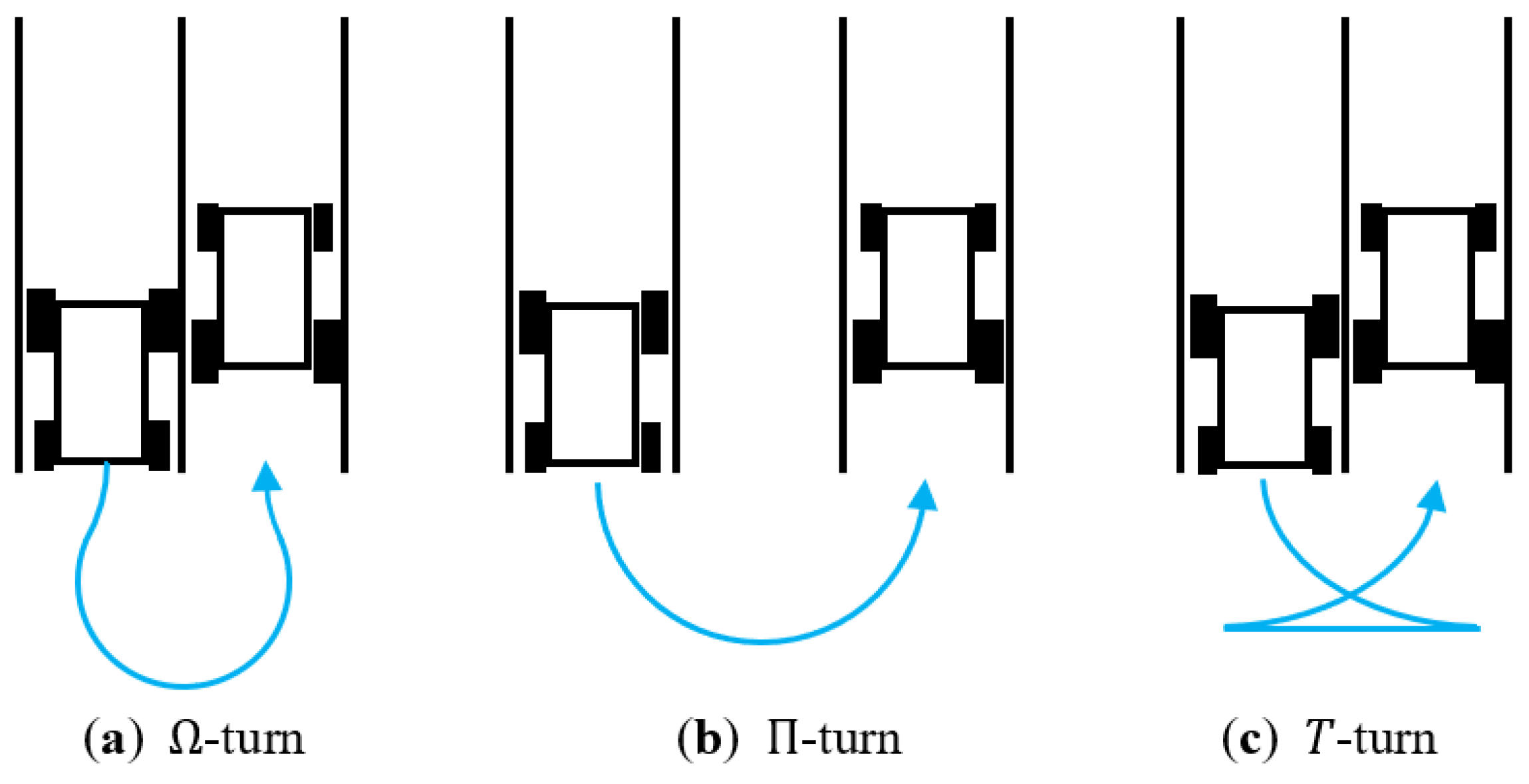
Once the optimal tracking trajectory has been optimized, the desired agricultural machinery operational efficiency is assumed to be determined accordingly, and a path-tracking algorithm will be utilized to realize this pre-determined agricultural machinery operational efficiency, by tracking the optimized trajectory with the best accuracy. Specifically, the execution of the transports along the optimized trajectory from the operational layer is typically an autonomous navigation problem, or a path-tracking problem, which is an important challenge that agricultural applications have in common [14]. The optimized trajectories are usually composed of two major categories: the working trajectories within the tracks, and the non-working trajectories in the headlands. Automatic steering systems based on path-tracking algorithms have become an important tool for guidance on a track, with accuracy in the range of centimeters; the transition from one track to another in the headlands must also be conducted exactly. There are many turning types proposed by research on the headlands. The most commonly used maneuvers are: (a) loop turn (-turn); (b) double-round-corner turn (-turn); (c) reverse turn (-turn) [15]. For more types of turning maneuvers, interested readers can refer to [16,17].
The main goal of the traditional path-tracking algorithm in agriculture is to control the agricultural machinery, in order to track a pre-determined path with best accuracy by calculating the optimal control variables. The path-tracking procedure can therefore be regarded as a control layer which aims to minimize deviations of the autonomous agricultural machinery from the pre-determined trajectory. As it is moving along the trajectory, the autonomous agricultural machinery executes farming tasks such as tillage, harvesting, and application of inputs such as nitrogen, seeds, and pesticides [18].
Most path-tracking control algorithms in agriculture only focus on how to improve the trajectory-tracking performance of autonomous agricultural machinery on both straight-line parallel tracks and headland turning curves, in the face of slippage and other disturbances [19]. These algorithms are denoted as traditional path-tracking algorithms. Nonlinear Model Predictive Control (NMPC) is a promising control algorithm, which can solve path-tracking problems in agricultural operations with high accuracy [20]. Model Predictive Control (MPC) refers to a class of computer control algorithms that utilize an explicit process model to predict the future responses of a plant [21]. Nonlinear-model-based MPC is denoted as NMPC. The main difference from conventional control methods is that NMPC uses an online control law in a receding horizon fashion [22], and this control law is the optimal solution obtained by solving an online optimization problem. Since its inception in the 1970s, MPC has been successfully applied to complex industrial processes, and it has shown great potential for handling complex constrained-optimization control problems [23,24]. More detailed descriptions of model predictive control can be found in [25]. Thanks to the development of microprocesses, the NMPC algorithm can nowadays also be applied to agricultural applications [4,26].
However, this NMPC-based path-tracking algorithm can only optimize the control performance of the autonomous agricultural machinery while the machinery is in motion, and the agricultural machinery operational efficiency is only a by-product of the control performance with respect to a pre-determined trajectory. In other words, the traditional NMPC path-tracking algorithm is unable to optimize the global performance of the whole system defined in the operational layer—like agricultural machinery operational efficiency—directly online.
Specifically, the use of NMPC is typically in a two-layer structure: the upper operational layer first optimizes a tracking trajectory based on the global performance of the whole system, such as improving the agricultural machinery operational efficiency; and then the lower NMPC control layer receives this optimized trajectory, and it tries its best to track this given trajectory by solving online optimization problems. This hierarchical two-layer structure has its own limitations: the path-planning procedure is determined offline, and therefore cannot predict future unknown disturbances which may occur in arable farming; and the optimized path is only a sub-optimal trajectory, considering the real-time disturbances. The NMPC control layer can overcome disturbances in order to perfectly track the pre-determined trajectory; however, this control performance may unexpectedly degrade the potential agricultural machinery operational efficiency, because the aim of the optimization problem in NMPC is to minimize the tracking errors, not to improve the agricultural machinery operational efficiency. In this paper, we introduce the concept of “beneficial disturbances” to show that an ideal path-tracking algorithm should have the ability to improve agricultural machinery operational efficiency directly in the control layer online.
The Robotic Operation System (ROS), on the other hand, can also realize autonomous navigation by the embedded Navigation Stack [27]. The Navigation Stack is a package of the ROS that performs SLAM (Simultaneous Localization and Mapping) and path planning, along with other functionalities for navigation [28]; the ROS will then send control instructions to a lower controller, like PID (proportional integral derivative) controller, to implement control actions [29]. Unlike NMPC, where the reference trajectory is determined offline, ROS-based navigation can update the global path in real-time, which enables it to improve the operational performance. More details of the autonomous navigation realized by the ROS can be found by referring to [30,31,32]. However, ROS-based navigation also has limitations: (1) it is a two-layer structure, where the upper layer is the Navigation Stack in the ROS aiming to obtain the updated global path, and the lower layer is the controller aiming to implement the control actions. As the time scales of the upper layer and the lower layer are not equal, the update of the global path is executed at a certain time interval which is greater than the time interval of the lower controller. Thus, during the control of the lower layer, it can only optimize the control performance of the given trajectory, and the optimization towards the operational performance is ignored; (2) Navigation Stack is powerful, yet it requires fine tuning of parameters to optimize its performance, and this tuning task is not as simple as it looks, and is potentially time-consuming [33]. To summarize, the Navigation Stack technique in the ROS has the potential to obtain better operational performance by updating the global path, but the large update interval and the parameter tuning tasks mean that the operational performance remains sub-optimal.
Thus, it is not enough for the path-tracking algorithm to track a pre-determined trajectory perfectly, regardless of the disturbances in NMPC, or to track an updated trajectory at a certain interval by the lower controller. An ideal path-tracking algorithm should also take the global performance of the whole system defined in the operational layer (denoted as operational performance for brevity), like agricultural machinery operational efficiency, into consideration to guide the movements of the autonomous agricultural machinery. This kind of path-tracking algorithm is denoted as an intelligent path-tracking algorithm, and was the main motivation behind this paper.
From the perspective of control theory, the optimizing control technique—which integrates the optimization in the operational layer with the control in the control layer—has the potential to improve the operational performance in the control layer online. This optimizing control idea is still absent in agricultural operation. Introducing this optimizing control concept into autonomous agricultural machinery should help to improve agricultural machinery operational efficiency online.
The main contribution of this paper is to propose a new kind of intelligent path-tracking algorithm, named Efficiency-oriented Model Predictive Control (EfiMPC), to realize optimizing control of autonomous agricultural machinery. EfiMPC can not only consider the control performance towards a given trajectory, but can also consider the global performance objective defined in the operational layer—like agricultural machinery operational efficiency—in the control layer online, by a nested optimization structure. Thus, EfiMPC can further improve agricultural machinery operational efficiency based on a given tracking trajectory, and the intended farming tasks can be completed successfully in the meantime.
2. Vehicle Kinematic Model
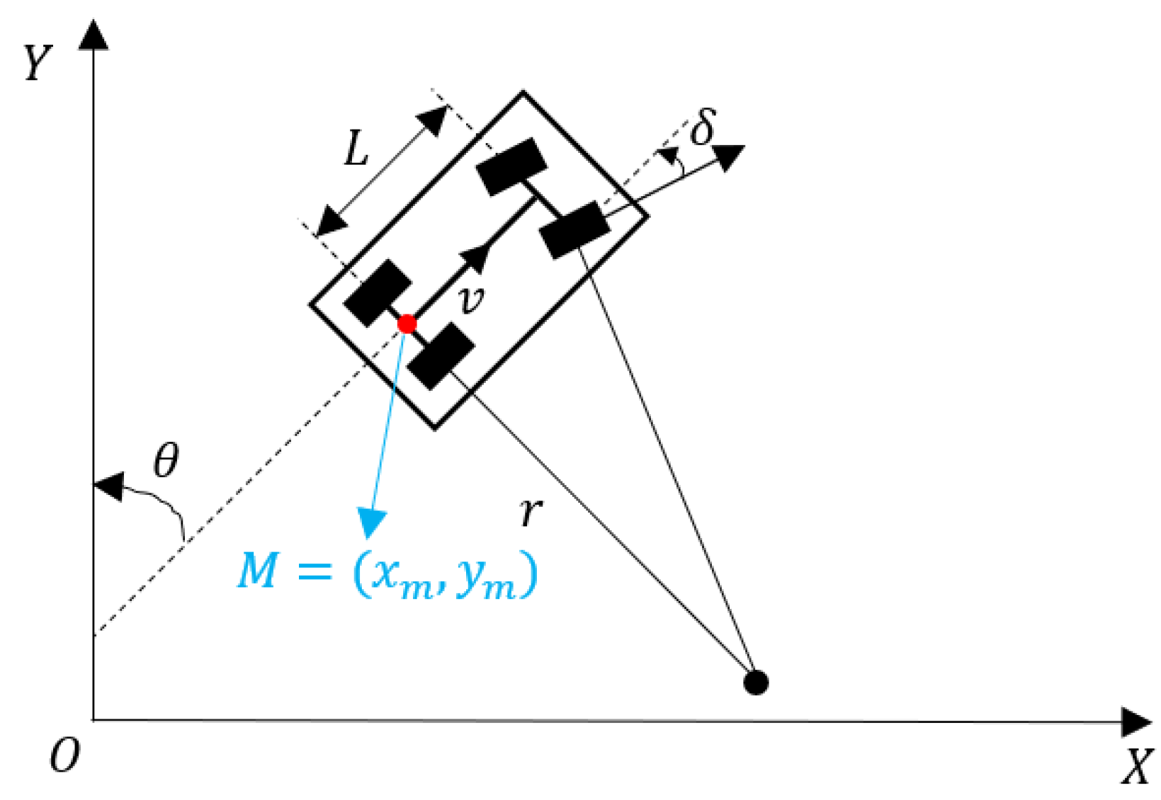
Autonomous agricultural machinery could be modelled with a high-fidelity nonlinear dynamic model, in which every force that affects the system is considered. However, this kind of complicated model would require modeling of the environments: for example, slipping, which depends on soil moisture and tire properties [34]. In addition, using this strict model with Nonlinear Model Predictive Control (NMPC) would lead to difficulties with computational capacity. As we only tried to demonstrate the effectiveness of the proposed Efficiency-oriented Model Predictive Control (EfiMPC) algorithm for its application in autonomous agricultural machinery, a simplified model is qualified in this paper. A more complicated nonlinear model with environmental interactions will be investigated in our future research. The kinematic model of autonomous agricultural machinery is briefly illustrated in Figure 1.
As shown in Figure 1, a simplified kinematic model was applied to describe the motion of autonomous agricultural machinery in Cartesian coordinates . The red point, , is the mid-point of the rear axle of a vehicle representing the position of the autonomous agricultural machinery in the arable field. The coordinates of are . represents the heading angle of the vehicle; represents the steering angle of the front wheel; represents the velocity; represents the length of the vehicle wheelbase; and represents the turning radius.
The derivative of the heading angle is given by , where . Thus, we have [35]:
The derivative of represents the velocity in the axis, and it is given by:
The derivative of represents the velocity in the axis, and it is given by:
Then, the kinematic model of the autonomous agricultural machinery is given as follows:
where the system states are , and the control inputs are , where the superscript represents the transpose of a vector. In addition, Equation (4) can be expressed as , for brevity.
3. Control Algorithm
3.1. Problem Statement
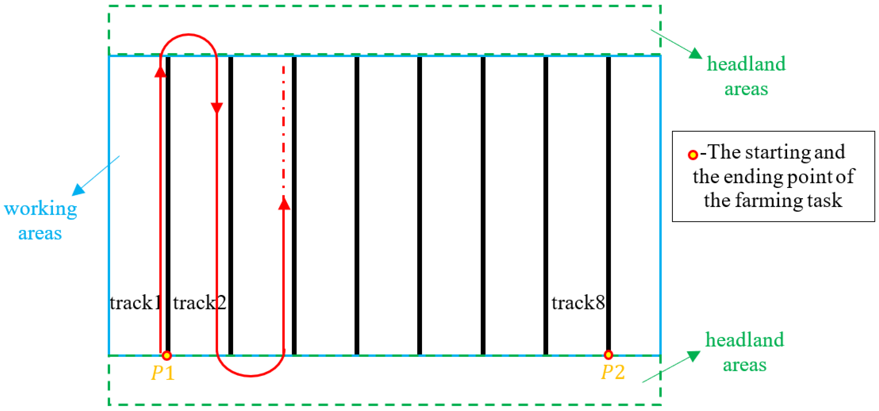
In a field operation in agriculture, the autonomous agricultural machinery executes farming tasks while it is moving [36], and a tracking trajectory is usually optimized in the operational layer before the agricultural vehicle starts to work. The farming task considered in this paper was simplified into working from track1 to track8, as shown in Figure 2, with the requirement that all eight tracks should be covered thoroughly by the vehicle once.
As shown in Figure 2, there were two distinct categories in this agricultural field: one category consisted of the working areas where the autonomous agricultural machinery executed tasks while moving along the tracks (the blue rectangular areas); the other category consisted of the headland areas, where the autonomous agricultural machinery only executed turning maneuvers from one track to another (the dashed-green rectangular areas). The respective aims in these two categories were also different from one other: when working in the tracks, the autonomous vehicles were expected to cover the tracks perfectly, in order to execute their farming tasks successfully; when moving in the headlands, the autonomous vehicles were expected to spend less time on these non-working areas. All eight of the tracks were required to be visited once via the headland areas. There have been many useful maneuvers in the headlands proposed by different researchers. The three most commonly used maneuvers are illustrated in Figure 3: (a) -turn; (b) -turn; (c) -turn. Optimal maneuvers in the headlands are determined by the specific environment of the operation field, which was not a major concern of this paper; thus, only the -turn maneuvers were used in the given optimized trajectory in Figure 2, to illustrate the ideas of the newly proposed Efficiency-oriented Model Predictive Control algorithm.
In order to improve the agricultural machinery operational efficiency, which was the global objective of the whole system considered in this paper, the operational layer tried to minimize the total traveling time of the autonomous agricultural machinery, from the starting point of track1 to the ending point of track8, so that the farming tasks could be completed successfully while it was moving. Thus, the tracking trajectory was optimized in the operational layer, and the agricultural machinery operational efficiency objective and farming constraints (the constraints of the autonomous vehicles, the constraints of the obstacles in the field, etc.) were considered during optimization. Then, this optimized trajectory was sent to the control layer in the autonomous agriculture machinery, to steer its movements. In this way, the agricultural objective in the operational layer was translated into a control objective in the control layer.
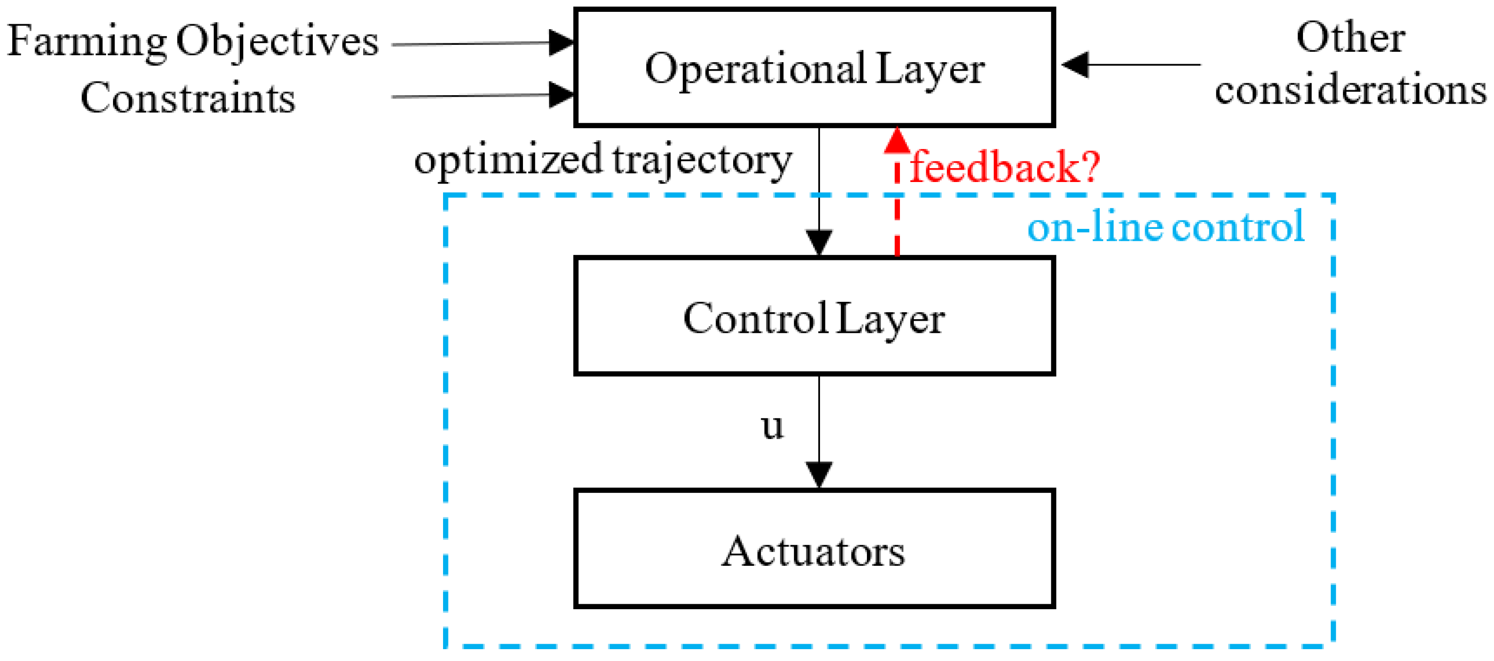
The hierarchical two-layer structure of this typical control strategy is illustrated in Figure 4. From the perspective of the control theory, however, there needed to be a feedback mechanism from the control layer to the operational layer, so that this feedback could help to further improve the agricultural machinery operational efficiency online during the working periods of the autonomous vehicle.
We assumed that the optimized trajectory had already been given by the operational layer, and that it was denoted as the red trajectory in Figure 3 (as the specific construction of this tracking trajectory was not the concern of this paper, we assumed that this tracking trajectory had already been given offline). Then, the control layer of the agricultural vehicle would try its best to track this pre-determined trajectory during its motion, and the autonomous agricultural machinery would execute agricultural tasks in the meantime.
Thus, the problem of the autonomous agricultural machinery control became an optimal path-tracking problem, defined as follows:
where and were the initial and the ending-time instant, respectively, of the agricultural operation; was the system state at the current sample instant, ; was the predicted system state of the open-loop system; was the optimized trajectory received from the operational layer; was the dynamic model of the autonomous agricultural machinery defined in Equation (4); and were the constraints of the system states and control inputs, respectively. was a -neighborhood of the ending point in the agricultural field, as shown in Figure 3, and was defined as follows:
where was a norm computation; was a parameter bigger than 0, and it was defined as in this paper.
In Equation (5), was a cost function representing the deviation from the given tracking trajectory, , and it was defined as follows:
where and were symmetric positive semi-definite weighting matrices, and .
The disturbance considered in the simulation was , adding to the state at the closed-loop system, where was a bounded disturbance satisfying:
and the updated state at the closed-loop system satisfied , where was the open-loop predicted state. The sample interval considered in this paper was where .
Some researchers have focused on how to plan the optimal trajectory, , while others have focused on how to control the agricultural vehicle to track this optimized trajectory perfectly; however, few researchers have focused on how to integrate optimization and control, to improve the operational layer performance online (the agricultural machinery operational efficiency considered in this paper). Integration of optimization and control is one of the most popular research topics in control theory nowadays.
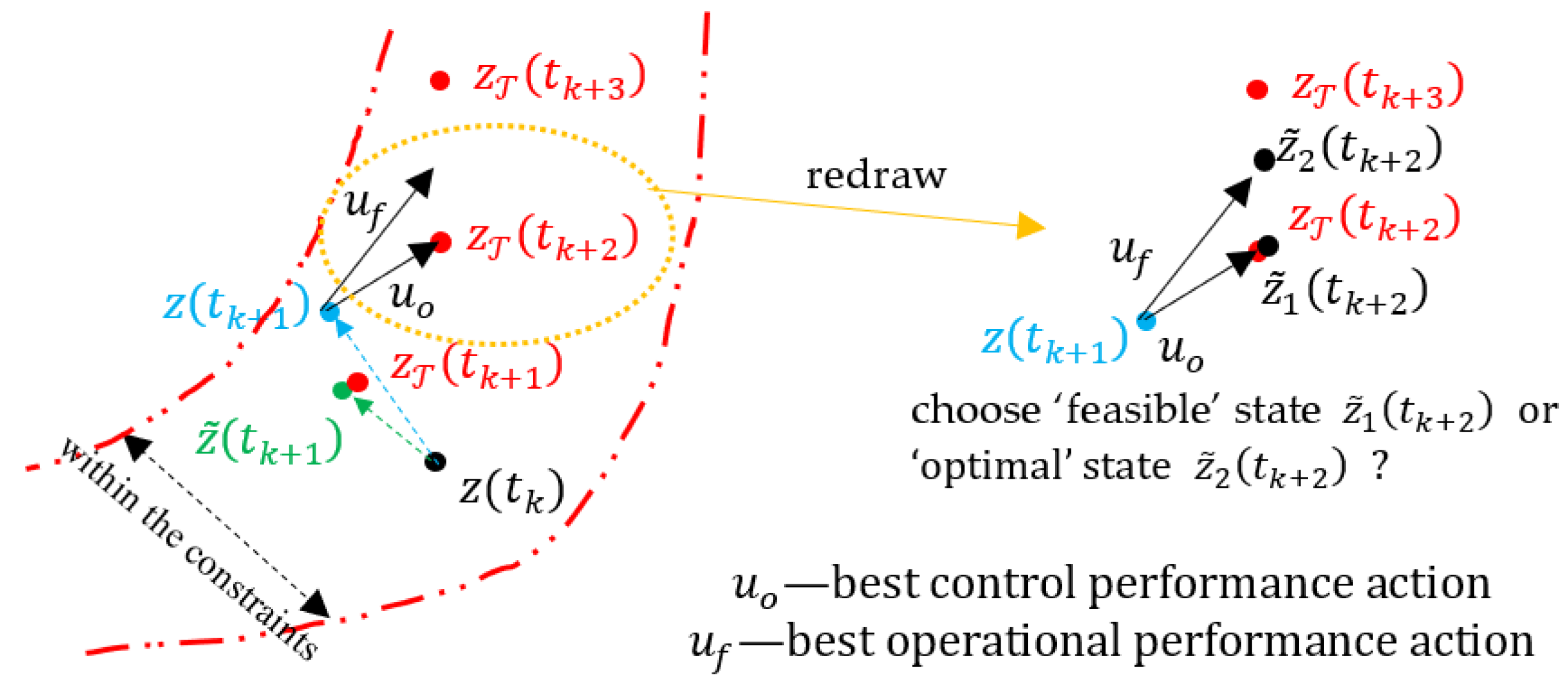
In this paper, we propose a new kind of path-tracking algorithm, named Efficiency-oriented Model Predictive Control (EfiMPC), which can improve agricultural machinery operational efficiency in the control layer online. One of the basic motivations of EfiMPC is that it can take advantage of “beneficial disturbance” to improve the performance defined in the operational layer. The brief ideas of beneficial disturbance are illustrated in Figure 5.
As shown in Figure 5: is the system state at the current sample instant, ; is the predicted state of the open-loop system; is the closed-loop state at the next sample instant, , influenced by the disturbance . This disturbance pushes the system state towards the tracking points, and . Then, the controller will determine an optimal solution, , to track at the sample instant, . This optimal solution, , will result in a predicted state, , which can perfectly track . There exists another feasible solution, , which steers the predicted state into , and this is reachable because the beneficial disturbance, (, is not reachable from ). The question is: which one is the preferred solution? From the perspective of tracking performance, there is no doubt that is preferable, because is nearer to ; however, from the perspective of the operational layer performance—which wants to improve the agricultural machinery operational efficiency— is preferable because: (1) it satisfies the constraints and meets the requirements of the farming tasks, and (2) it saves working time, because it moves further in the track, and the agricultural machinery operational efficiency can be improved accordingly.
The traditional NMPC algorithm is unable to consider the objective defined in the operational layer, and it cannot make use of beneficial disturbances to improve the agricultural machinery operational efficiency online; whereas the proposed EfiMPC algorithm is able to consider the operational layer performance in the control layer online, to further improve the agricultural machinery operational efficiency, which makes the autonomous agricultural machinery more intelligent.
3.2. Traditional NMPC Algorithm
The basic idea of traditional Nonlinear Model Predictive Control (NMPC) is to predict the future responses of a nonlinear system under control actions, while the constraints are satisfied, and a given cost function is optimized online, in order to obtain optimal controls in a receding horizon fashion. Thus, NMPC uses finite-horizon-based online optimization problems to replace Equation (5), which is unrealistic in practice due to its large optimization horizon.
Given an optimized tracking trajectory, , from the operational layer, the NMPC controller solves the following optimization problem online at every sample instant, , to control the autonomous agricultural machinery:
where: is the prediction horizon; is the current sample instant; is the cost function defined in Equation (6); is the dynamic model of the autonomous vehicle defined in Equation (4); and are the constraints of the system states and control inputs, respectively, and they satisfy:
The solution to Equation (7) is the optimal control . In this paper, was a piece-wise constant control sequence, satisfying:
Only the first control action in will be implemented into the system in the closed-loop perspective, and the optimization procedure will be repeated with the updated system state, , at the next sampling instant . The control procedure will be terminated once the system state becomes the end state in Figure 2, which means .
The NMPC controller defined in Equation (7) is a two-layer structure, as shown in Figure 4, and there are two main issues: (1) the objective function defined in Equation (7) is the control performance, and the agricultural machinery operational efficiency defined in the operational layer cannot be optimized directly; (2) the given tracking trajectory, , is optimized offline, which will result in sub-optimal operation.
To address the above two issues, a feedback mechanism between the control layer and the operational layer should be introduced to integrate control and optimization. In this way, the agricultural machinery operational efficiency can be further improved online. In addition, the given tracking trajectory, , should be regarded as one feasible solution, and better solutions could be optimized online, taking the beneficial disturbances into account.
3.3. Efficiency-Oriented Model Predictive Control Algorithm
3.3.1. Ideas of Efficiency-Oriented Model Predictive Control
Efficiency-oriented Model Predictive Control (EfiMPC) aims to solve an online optimization problem at every sample instant in a receding horizon fashion, and is defined as follows:
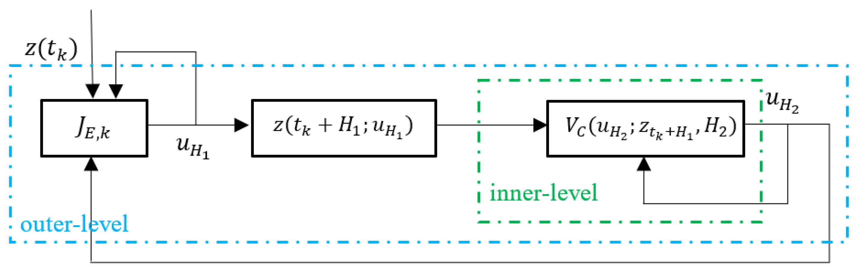
where most definitions of parameters are the same as those defined in Equation (7). is an objective function to measure the performance of the agricultural machinery operational efficiency defined in the operational layer. is an objective function to measure the performance of the control performance defined in the control layer. and are the constraints of the system states and control inputs, respectively, in the outer-level optimization problem. and are the constraints of the system states and control inputs, respectively, in the inner-level optimization problem. is the terminal constraint of the outer level. is the closed-loop state of the system at the current sample instant , and are the predicted states of the open-loop system. is the prediction horizon defined in Equation (7), and it is divided into two parts: and ; thus, the control actions have also been divided into two parts: and is the optimal solution to Equation (8), and is the corresponding optimal state trajectory.
The EfiMPC strategy defined in Equation (8) is intrinsically a nested optimization problem [37], where the outer-level optimization problem optimizes the performance defined in the operational layer by , and the inner-level optimization problem optimizes the performance defined in the control layer by . In this way, the predicted dynamics resulting from the control objectives can be assessed by the operational layer objectives online; thus, EfiMPC builds feedback between the control layer and the operational layer with the help of this nested structure. See Figure 6 for the nested structure of EfiMPC.
As shown in Figure 6, the independent variable was used to optimize the performance of the operational layer directly, and the independent variable was used to control the system from the perspective of the control performance, based on the optimized terminal state . Thus, the inner level focused more on the stability of the system, the outer level focused more on the optimality of the agricultural machinery operational efficiency, and together were able to realize optimizing control by considering operational layer performance in the control layer online.
At every sample instant, , EfiMPC solved the optimization problem (8) repeatedly, and then it executed the first control action, , into the closed-loop system. The resulting implicit closed-loop input profile, , realized by the receding horizon fashion, had the following form:
The closed-loop system had a corresponding closed-loop performance, , measuring the objective of the operational layer , where was the starting instant of the agricultural operation, and was the ending instant of the agricultural operation. EfiMPC is a receding horizon strategy, which approximates the ideal optimal control problem, and the ideal optimal control problem has a corresponding optimal solution which will result in an optimal operational performance, , indicating the ideal optimal agricultural machinery operational efficiency. The traditional NMPC strategy, and the proposed EfiMPC strategy, both try to realize this ideal performance, . The main difference is that EfiMPC can use a feedback mechanism to optimize online, to render it closer to (increasing the agricultural machinery operational efficiency online, in this paper); while in NMPC, there are no such feedbacks, and it can only optimize the control performance. The operational performance is only a byproduct of the control performance in NMPC, and this performance could be degraded by real-time disturbances.
3.3.2. The Application of Efficiency-Oriented Model Predictive Control
The objective in the operational layer considered in this paper was to maximize the agricultural machinery operational efficiency; it was simplified into minimizing the working time from the start point to the end point , as shown in Figure 2. Furthermore, the farming tasks had to be completed by autonomous agricultural machinery.
However, in the EfiMPC strategy defined in Equation (8), it was inappropriate to directly use the working time as the objective function , because the receding horizon strategy used in EfiMPC rendered the prediction horizon, , fixed during the optimization. To overcome this limitation, EfiMPC translated the objective of “minimize the working time in a certain field” into the objective of “maximize the working distance within a certain working time”. In other words, the following three objectives were expected to be equivalent:
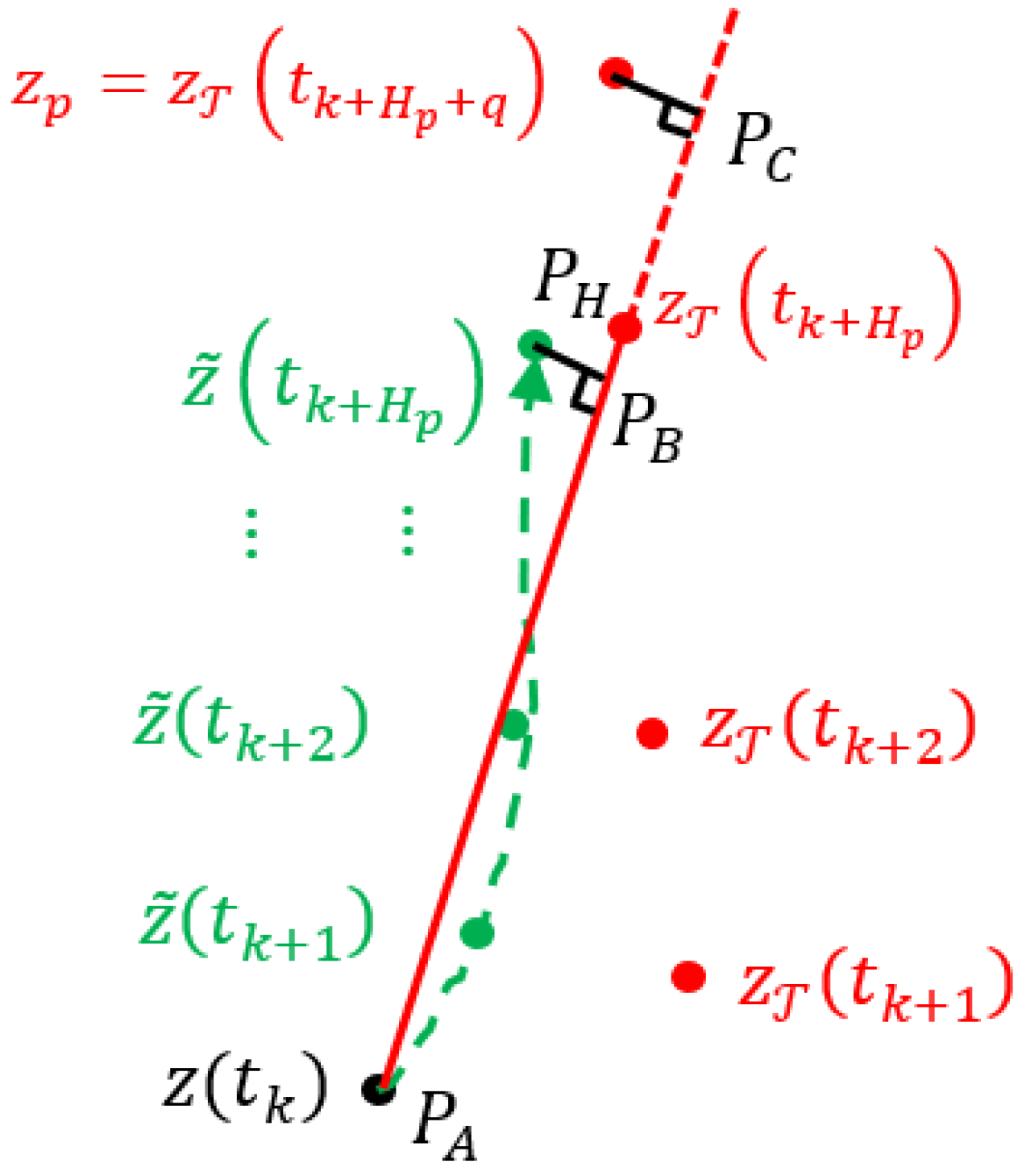
where is the working time of the autonomous vehicle, spent from to , in Figure 2; is the length of the effective distance the autonomous vehicle covered within the prediction horizon; ; is the terminal state at the end of the prediction horizon; and is a pseudo-state which helps to maximize the effective distance . The ideas of the effective distance , as well as the pseudo-state , are illustrated in Figure 7.
As shown in Figure 7: is the state of the closed-loop system at the current sample instant ; are the predicted system states of the open-loop system; are the tracking points at the given tracking trajectory; denoting as point ; denoting as point ; and point being the projection of into the straight line . Then, the length of the line segment, , is denoted as the effective distance . This effective distance represents the working distance of the autonomous agricultural machinery covered in the tracks within the prediction horizon . A larger working distance within a certain time interval, , indicates a shorter time spent in agricultural operation, and thus is verified.
However, the tracking control of towards will restrict the terminal state within a small neighborhood of , and the optimization of will suffer accordingly. This limitation implies that the control performance may degrade the optimization performance of the operational layer.
Thus, in order to realize the optimization of the effective distance, , a pseudo-point is introduced, and it satisfies , where is a non-negative integer. In essence, this pseudo-point is an unreachable tracking point that cannot be reached from within the prediction horizon , and it can help optimize the length of beyond . See Figure 7 again: point is the projection of the pseudo-point into the extension of the line segment , and it satisfies . Thus, the maximization of effective distance is identical to the minimization of , and the equivalence of has been verified accordingly.
To summarize, the objective of minimizing the working time has been converted into the objective of minimizing the distance between the terminal state and the pseudo-state , and the resulting EfiMPC controller, is thus defined as follows:
where most definitions of parameters are the same as those defined in Equation (8); is a terminal constraint in the outer level, which restricts the outer-level terminal state within a neighborhood of ; and are symmetric positive semi-definite weighting matrices.
In Equation (9), EfiMPC divides the control variables into two parts: in the outer-level optimization, and in the inner-level optimization. The outer level focuses mainly on improving the operational performance, and the inner level guarantees that the optimized control action can also satisfy the control performance.
The farming tasks were not specifically defined in this paper; instead, they are indicated by the constraints defined in Equation (9). Thus, once the constraints in Equation (9) were satisfied, it was assumed that the corresponding farming tasks had also been completed successfully. The detailed constraints indicating the farming tasks are defined as follows:
where is the parameter defined in , and this also represents the maximum lateral deviations of the autonomous agricultural machinery while in motion.
4. Results
In order to demonstrate the effectiveness of the proposed path-tracking algorithm, Efficiency-oriented Model Predictive Control (EfiMPC), a case study of the agricultural operation defined in Figure 2 was used for simulation here. The ultimate objective was to improve agricultural machinery operational efficiency, which meant that the autonomous agricultural machinery had to execute the required farming tasks in the tracks successfully, while the working time spent from the starting point to the ending point had to be minimized in the meantime. The ideal shortest working time of the autonomous agricultural machinery was 108.5 s in this case study.
The EfiMPC algorithm defined in Equation (9), and the traditional NMPC algorithm defined in Equation (7), were used as the comparative algorithms for the autonomous agricultural machinery here, and the specific parameters and setups were defined as follows: the sampling interval s; the prediction horizon, ; the outer-layer horizon, ; the inner-layer horizon ; the pseudo-point parameter ; the minimum steering angle of the front wheel, rad/s; the maximum steering angle of the front wheel, rad/s; the minimum velocity of the vehicle, m/s; the maximum velocity of the vehicle, m/s; the weighting matrices, , , and , where represented the diagonal matrix; the dimension of the vehicle, , was 2; the dimensions of the fields and the tracks were also 2 (Cartesian coordinates ); the length of a single track was 18 m, and the distance between two neighboring tracks was 1.5 m.
The optimization of the outer-level problem, with respect to in Equation (9), was realized by metaheuristic algorithms, such as the OSPO algorithm [38]; the optimization of the inner-level problem, with respect to in Equation (9), was realized by deterministic algorithms, such as the sequential quadratic programming [39] embedded in the fmincon algorithm in MATLAB. The optimization of Equation (8) was also realized by the fmincon algorithm in MATLAB.
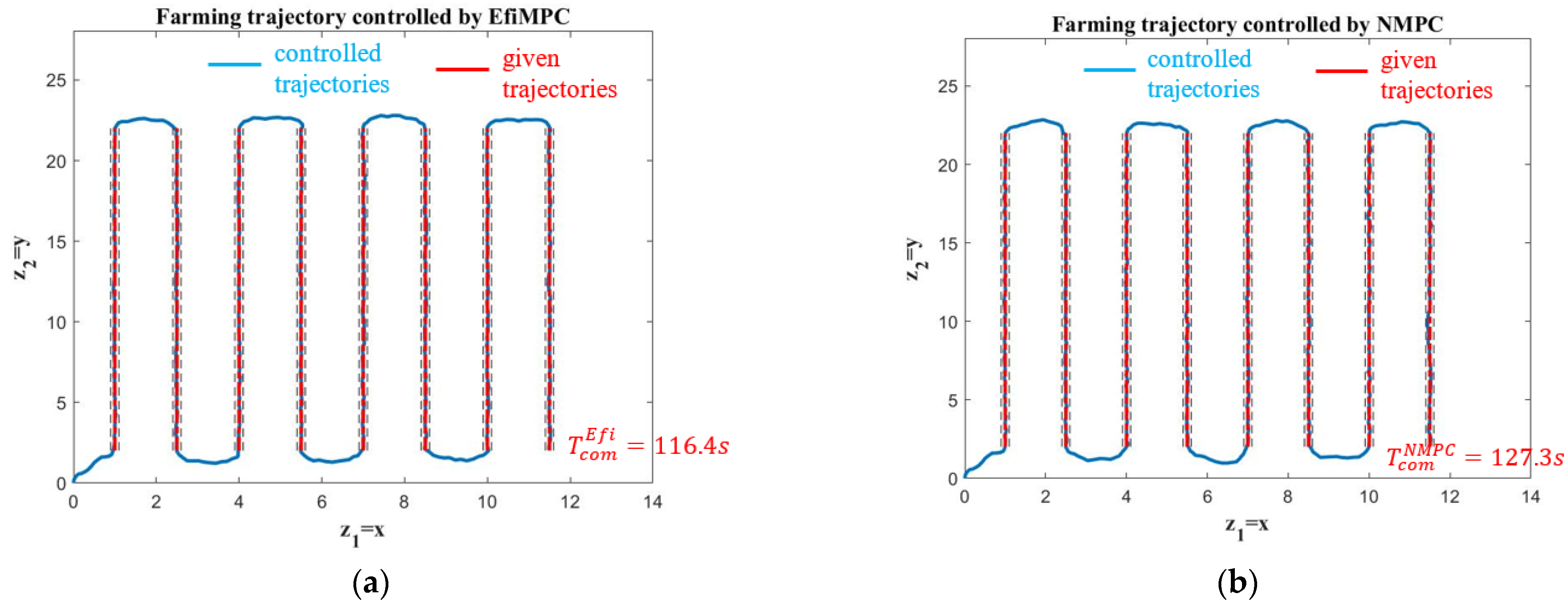
The simulation results of the working trajectories realized by EfiMPC and NMPC are illustrated in Figure 8a,b, respectively. Both control strategies executed the farming tasks successfully from the start point to the end point , because they satisfied all the constraints during the operation. However, the amount of working time spent by EfiMPC and NMPC differed: the autonomous agricultural machinery controlled by EfiMPC took s to complete the farming tasks, while the autonomous agricultural machinery controlled by NMPC took s to complete the same farming tasks. Thus, the agricultural machinery operational efficiency realized by EfiMPC was better than that by NMPC, and the specific improvement, by using the EfiMPC algorithm, was 8.56% compared to the NMPC algorithm.
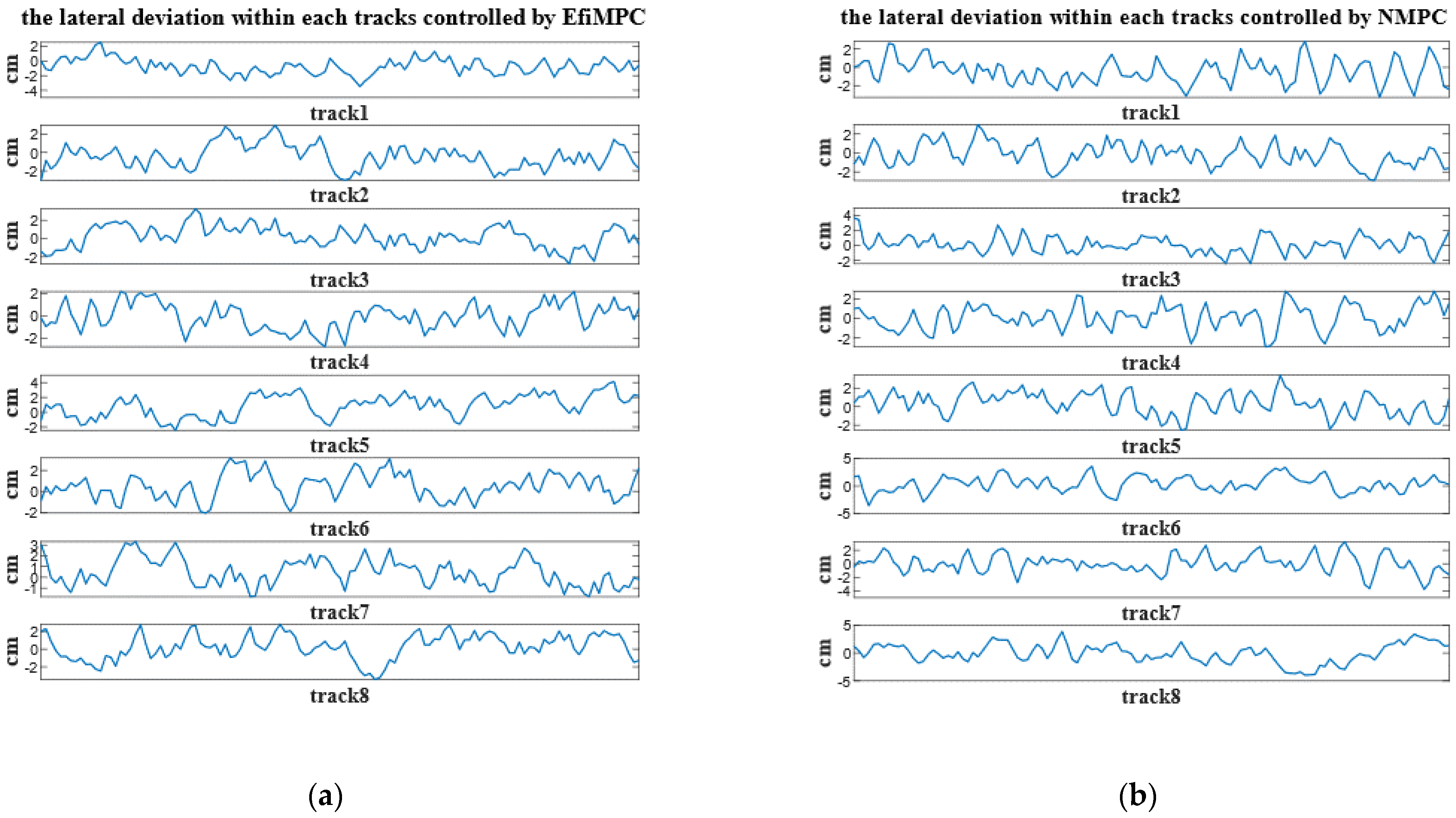
To finish the farming tasks quickly is not enough; it is also necessary to satisfy the farming requirements during the operations. The farming requirements considered in this paper were mainly to keep the lateral deviations from the tracks smaller than 5 cm (which are denoted by the regions between dashed lines in Figure 8); the detailed lateral deviations controlled by EfiMPC and NMPC for each track are illustrated in Figure 9a,b, respectively.
The maximum lateral deviation of the movements in the working tracks controlled by EfiMPC was 4.1363 cm, while the maximum lateral deviation of the movements in the working tracks controlled by NMPC was 3.97 cm. The average lateral deviations of the movements in the working tracks controlled by EfiMPC and NMPC were 1.1161 cm and 1.1118 cm, respectively. Thus, from the lateral deviation perspective, NMPC outperformed EfiMPC. The reason for this phenomenon was that EfiMPC sacrificed some tracking performance in order to realize better agricultural machinery operational efficiency, defined in the operational layer. As the lateral deviation was still within the constraints (4.1363 cm is smaller than 5 cm), the kind of sacrifice made by EfiMPC in this case was worthwhile, in order to improve the agricultural machinery operational efficiency.
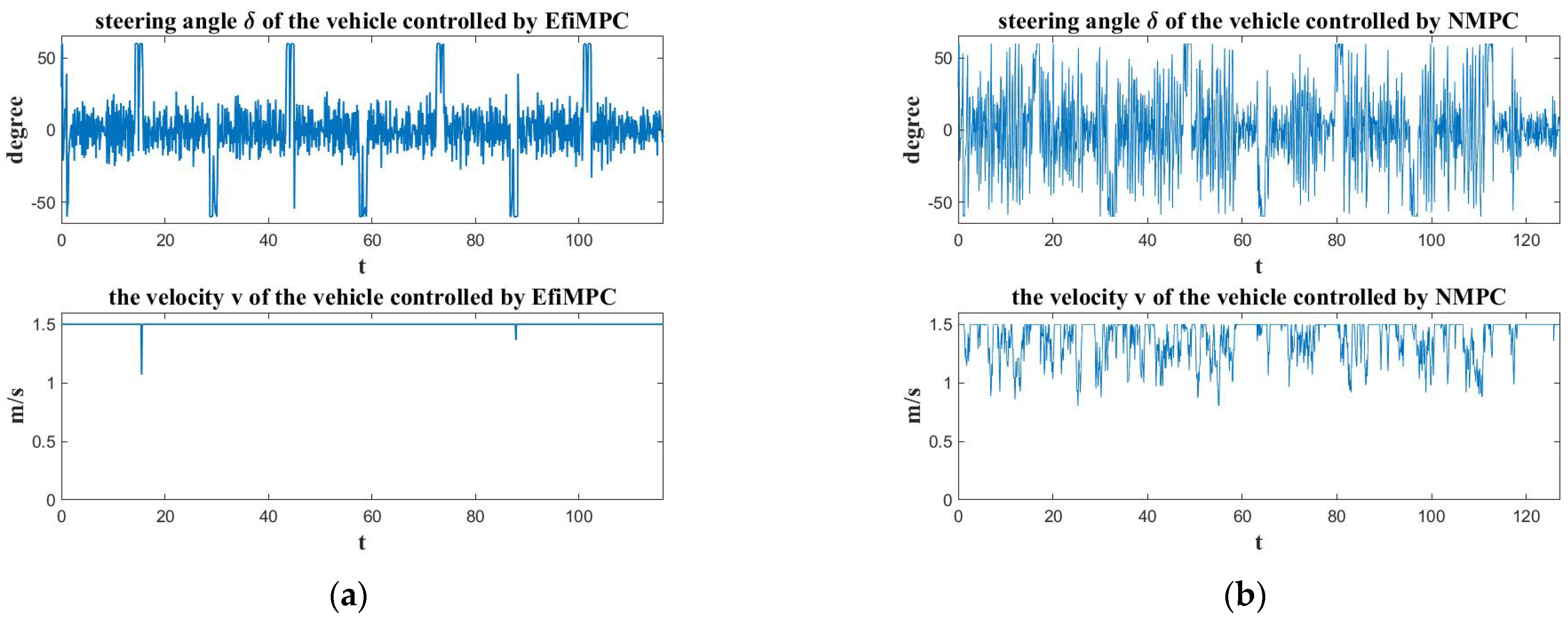
The control actions of the autonomous agricultural machinery, taken by EfiMPC and NMPC, are illustrated in Figure 10. As shown in Figure 10, the velocity of the vehicle controlled by EfiMPC was kept at the maximum value for most of the time, while the velocity of the vehicle controlled by NMPC may have deteriorated during the operation. This difference can be explained easily: the goal of EfiMPC was to improve the agricultural machinery operational efficiency, so the velocity of the vehicle was expected to be large; while the goal of NMPC was to track the tracking trajectory perfectly, so the vehicle may have had to slow down to track the neighboring tracking points, and it could make use of the beneficial disturbances. Furthermore, the steering angle δ of the vehicle was changed frequently in order to optimize the objectives defined in EfiMPC and NMPC, and one could define an additional constraint on the changing rate to alleviate these variations.
5. Discussion
According to the simulation results, it is clear that autonomous agricultural machinery controlled by an EfiMPC algorithm can achieve better agricultural machinery operational efficiency than that controlled by an NMPC algorithm, because the working time spent by EfiMPC was reduced by 8.56%.
Some readers may argue that the given tracking trajectory was not the optimal one, and thus degraded the performance of the NMPC; however, this was precisely another superior aspect of using EfiMPC. Specifically, given any feasible tracking trajectory which can complete the farming tasks while satisfying all the constraints, the EfiMPC algorithm can control the autonomous machinery to achieve better agricultural machinery operational efficiency by considering the operational performance in the control layer online; thus, a feasible tracking trajectory is enough for EfiMPC.
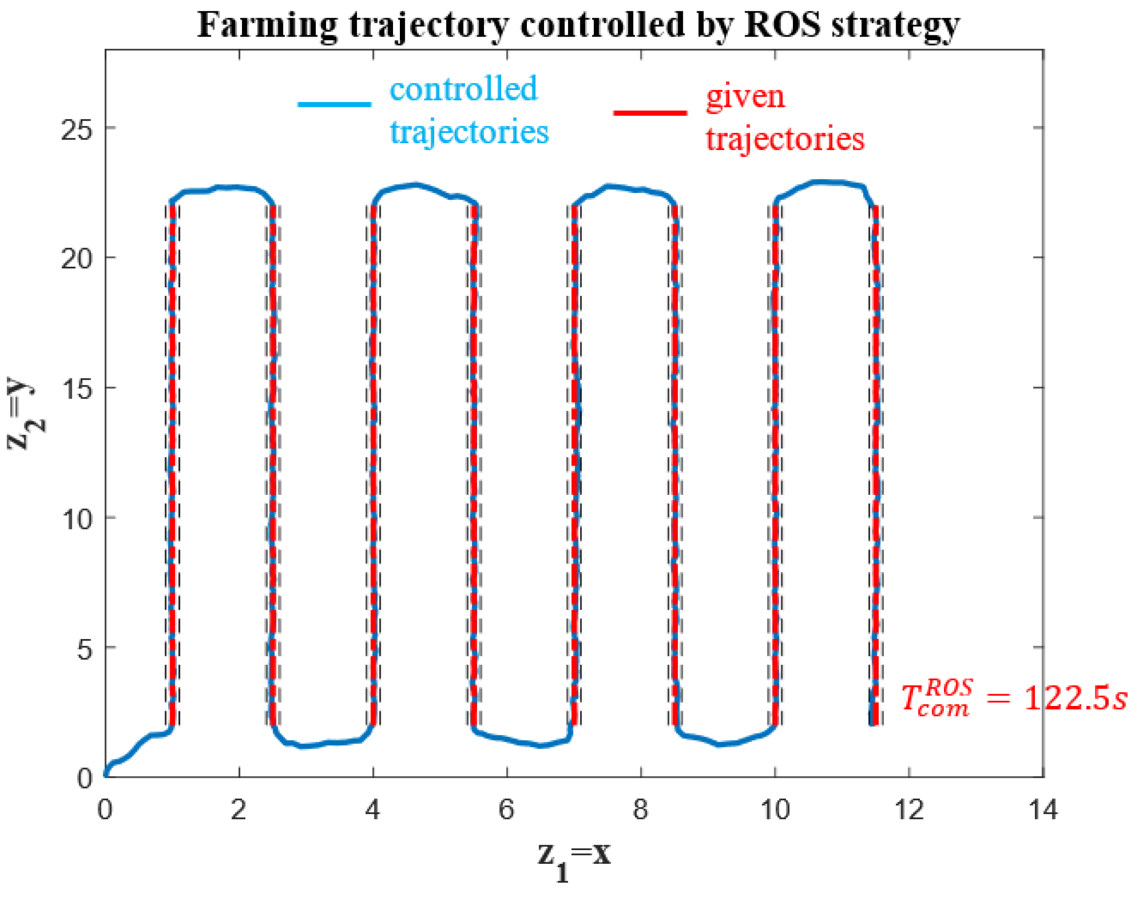
ROS-based navigation control has the ability to update the tracking trajectory online; thus, it also has the potential to improve operational performance. Here, we assumed that the Navigation Stack in the ROS could obtain the ideal trajectory, and that the updated trajectory would be sent to the lower controller. In the traditional ROS, the lower controller is typically a PID controller; here, we used an MPC controller to further improve the performance of the ROS. In this way, the ROS played the role of an upper layer, which updated the optimal tracking trajectory at a certain interval, and we defined this interval as 0.2 s, which was greater than s (because the upper layer typically has a lager time scale than that of the lower layer controller). The other parameter definitions were the same as those used in EfiMPC, and the simulation result is illustrated in Figure 11.
As shown in Figure 11, the working time spent by the ROS strategy was 122.5 s, which was better than the NMPC strategy (127.3 s), and worse than the EfiMPC strategy (116.4 s). The reason why the ROS strategy performed better than the NMPC strategy was that the ROS strategy was able to update the tracking trajectory to obtain a higher operational performance, while the NMPC strategy could only track an offline optimal trajectory. The reason why the EfiMPC strategy performed better than the ROS strategy was that, although the ROS strategy was able to update the tracking trajectory by a two-layer structure, the updating frequency was slower than the lower-layer controller; while for EfiMPC, it was able to optimize the control performance and the operational performance online simultaneously in one layer.
In addition, the parameter , used for pseudo-state , was in the simulation, without further explanations. Indeed, the value of can affect the performance of EfiMPC defined in Equation (9). If , EfiMPC will be degraded into tracking NMPC; a small value of has the potential to improve the agricultural machinery operational efficiency to a small extent, while the tracking performance can also be promised with a high accuracy; a large value of has the potential to improve the agricultural machinery operational efficiency to a larger extent, while the tracking performance (like lateral deviations) may suffer accordingly. Thus, the specific choice of the parameter could be further investigated. A balanced value, , was used in this paper, and more flexible values of , as well as their impacts, will be studied in our future research.
The main strength of EfiMPC is its nested structure, which can integrate the operational layer performance and the control layer performance into one framework. In this way, the optimizing control is realized by considering the operational performance in the control layer online. However, the nested optimization problem is intrinsically a complicated optimization problem, and an ideal optimization algorithm which can solve the EfiMPC problem, by promising performance fast, is desired. We will try to propose a specific optimization algorithm which aims to achieve this target in our future research.
This paper only uses a simulation to illustrate the superiority of the newly proposed path-tracking algorithm EfiMPC; the effectiveness of EfiMPC could be further tested in a real-world arable field. In our future studies, we will use EfiMPC to control autonomous vehicles in a real-world agricultural application.
6. Conclusions
This paper proposes a new kind of intelligent path-tracking algorithm, named Efficiency-oriented Model Predictive Control (EfiMPC), for autonomous agricultural machinery. EfiMPC can integrate the optimization in the operational layer and the control in the control layer, to further improve agricultural machinery operational efficiency online. The optimizing control property of EfiMPC is promised by the nested optimization structure, where the global performance of the whole system, defined in the operational layer, is mainly considered at the outer level, and the control performance is mainly considered at the inner level. In order to optimize agricultural machinery operational efficiency in a receding horizon fashion, ideas of effective distance and pseudo-point have been proposed in EfiMPC, and the optimization of agricultural machinery operational efficiency has been translated into the optimization of the distance between a terminal state and a pseudo-point. The simulation results show that EfiMPC can improve agricultural machinery operational efficiency by 8.56%, compared with the traditional NMPC algorithm; the effectiveness of the proposed EfiMPC has thus been demonstrated.
However, in this paper, the noises and model uncertainties have been ignored; state estimation and model parameter estimation techniques could be used to deal with these situations. In addition, the nested structure will increase the computation burden of the online optimization problem, and a suitable metaheuristic algorithm could be investigated to reduce the online computation. Furthermore, obstacle detection and avoidance systems are crucial to autonomous vehicles, and these systems could be integrated into EfiMPC by modifying the objective function.
This paper presents the initial idea of using EfiMPC in autonomous vehicles, which makes the autonomous agricultural machinery more intelligent by realizing optimizing control. Future studies could investigate the parameter defined in the pseudo-point, to further improve agricultural machinery operational efficiency. In addition, well-performed optimization algorithms suitable for the nested structure of EfiMPC could also be researched. Finally, EfiMPC could be used in a real-world agricultural application, to further investigate its properties.
Author Contributions
Conceptualization, J.X.; methodology, J.X.; software, J.X.; validation, J.X. and L.X.; formal analysis, J.X. and L.X.; investigation, J.X.; resources, J.X. and L.X.; data curation, J.X.; writing—original draft preparation, J.X.; writing—review and editing, J.L., R.G., X.L. and L.X.; visualization, J.X.; supervision, J.L., R.G., X.L. and L.X.; project administration, J.L., R.G., X.L. and L.X.; funding acquisition, J.L., R.G., X.L. and L.X. All authors have read and agreed to the published version of the manuscript.
Funding
This work was supported in part by the Ministry of Education—China Mobile Research Fund major project: No. MCM2020—J-2; in part by the National Natural Science Foundation of China under Grant 61973337; and in part by the U.S. National Science Foundation’s BEACON Center for the Study of Evolution in Action, under Cooperative Agreement DBI-0939454.
Institutional Review Board Statement
Not applicable.
Informed Consent Statement
Not applicable.
Data Availability Statement
Not applicable.
Conflicts of Interest
The authors declare no conflict of interest.
References
- Xiongkui, H.; Bonds, J.; Herbst, A.; Langenakens, J. Recent development of unmanned aerial vehicle for plant protection in East Asia. Int. J. Agric. Biol. Eng. 2017, 10, 18–30. [Google Scholar]
- Jensen, M.A.F.; Bochtis, D.; Sørensen, C.G.; Blas, M.R.; Lykkegaard, K.L. In-field and inter-field path planning for agricultural transport units. Comput. Ind. Eng. 2012, 63, 1054–1061. [Google Scholar] [CrossRef]
- Utamima, A.; Djunaidy, A. Agricultural routing planning: A narrative review of literature. Procedia Comput. Sci. 2022, 197, 693–700. [Google Scholar] [CrossRef]
- Ding, Y.; Wang, L.; Li, Y.; Li, D. Model predictive control and its application in agriculture: A review. Comput. Electron. Agric. 2018, 151, 104–117. [Google Scholar] [CrossRef]
- Moorehead, S.J.; Wellington, C.K.; Gilmore, B.J.; Vallespi, C. Automating Orchards: A System of Autonomous Tractors for Orchard Maintenance. In Proceedings of the IEEE/RSJ International Conference on Intelligent Robots and Systems (IROS) Workshop on Agricultural Robots, Algarve, Portugal, 7–12 October 2012. [Google Scholar]
- Spekken, M.; de Bruin, S. Optimized routing on agricultural fields by minimizing maneuvering and servicing time. Precis. Agric. 2013, 14, 224–244. [Google Scholar] [CrossRef]
- Bochtis, D.D.; Sørensen, C.G. The vehicle routing problem in field logistics: Part II. Biosyst. Eng. 2010, 105, 180–188. [Google Scholar] [CrossRef]
- Zhou, K.; Jensen, A.L.; Bochtis, D.; Nørremark, M.; Kateris, D.; Sørensen, C.G. Metric map generation for autonomous field operations. Agronomy 2020, 10, 83. [Google Scholar] [CrossRef] [Green Version]
- Han, X.; Lai, Y.; Wu, H. A Path Optimization Algorithm for Multiple Unmanned Tractors in Peach Orchard Management. Agronomy 2022, 12, 856. [Google Scholar] [CrossRef]
- Nørremark, M.; Nilsson, R.S.; Sørensen, C.A.G. In-Field Route Planning Optimisation and Performance Indicators of Grain Harvest Operations. Agronomy 2022, 12, 1151. [Google Scholar] [CrossRef]
- Khosravani Moghadam, E.; Vahdanjoo, M.; Jensen, A.L.; Sharifi, M.; Sørensen, C.A.G. An Arable Field for Benchmarking of Metaheuristic Algorithms for Capacitated Coverage Path Planning Problems. Agronomy 2020, 10, 1454. [Google Scholar] [CrossRef]
- Conesa-Muñoz, J.; Bengochea-Guevara, J.M.; Andujar, D.; Ribeiro, A. Route planning for agricultural tasks: A general approach for fleets of autonomous vehicles in site-specific herbicide applications. Comput. Electron. Agric. 2016, 127, 204–220. [Google Scholar] [CrossRef]
- Spekken, M.; de Bruin, S.; Molin, J.P.; Sparovek, G. Planning machine paths and row crop patterns on steep surfaces to minimize soil erosion. Comput. Electron. Agric. 2016, 124, 194–210. [Google Scholar] [CrossRef]
- Kraus, T.; Ferreau, H.J.; Kayacan, E.; Ramon, H.; De Baerdemaeker, J.; Diehl, M.; Saeys, W. Moving horizon estimation and nonlinear model predictive control for autonomous agricultural vehicles. Comput. Electron. Agric. 2013, 98, 25–33. [Google Scholar] [CrossRef]
- Bochtis, D.D.; Vougioukas, S.G. Minimising the non-working distance travelled by machines operating in a headland field pattern. Biosyst. Eng. 2008, 101, 1–12. [Google Scholar] [CrossRef]
- Sabelhaus, D.; Röben, F.; zu Helligen, L.P.M.; Lammers, P.S. Using continuous-curvature paths to generate feasible headland turn manoeuvres. Biosyst. Eng. 2013, 116, 399–409. [Google Scholar] [CrossRef]
- Backman, J.; Piirainen, P.; Oksanen, T. Smooth turning path generation for agricultural vehicles in headlands. Biosyst. Eng. 2015, 139, 76–86. [Google Scholar] [CrossRef]
- Finger, R.; Swinton, S.M.; El Benni, N.; Walter, A. Precision farming at the nexus of agricultural production and the environment. Ann. Rev. Resour. Econ. 2019, 11, 313–335. [Google Scholar] [CrossRef] [Green Version]
- Zhang, T.; Jiao, X.; Lin, Z. Finite time trajectory tracking control of autonomous agricultural tractor integrated nonsingular fast terminal sliding mode and disturbance observer. Biosyst. Eng. 2022, 219, 153–164. [Google Scholar] [CrossRef]
- Kayacan, E.; Kayacan, E.; Ramon, H.; Saeys, W. Learning in centralized nonlinear model predictive control: Application to an autonomous tractor-trailer system. IEEE Trans. Control Syst. Technol. 2014, 23, 197–205. [Google Scholar] [CrossRef]
- Qin, S.J.; Badgwell, T.A. A survey of industrial model predictive control technology. Control Eng. Pract. 2003, 11, 733–764. [Google Scholar] [CrossRef]
- Mayne, D.Q.; Rawlings, J.B.; Rao, C.V.; Scokaert, P.O.M. Constrained model predictive control: Stability and optimality. Automatica 2000, 36, 789–814. [Google Scholar] [CrossRef]
- Xi, Y.G.; Li, D.W.; Lin, S. Model predictive control—status and challenges. Acta Autom. Sin. 2013, 39, 222–236. [Google Scholar] [CrossRef]
- Forbes, M.G.; Patwardhan, R.S.; Hamadah, H.; Gopaluni, R.B. Model predictive control in industry: Challenges and opportunities. IFAC Pap. 2015, 48, 531–538. [Google Scholar] [CrossRef]
- Magni, L.; Raimondo, D.M.; Allgöwer, F. Nonlinear Model Predictive Control: Towards New Challenging Applications; Lecture Notes in Control and Information Sciences; Springer: Cham, Switzerland, 2009. [Google Scholar]
- Bersani, C.; Ouammi, A.; Sacile, R.; Zero, E. Model predictive control of smart greenhouses as the path towards near zero energy consumption. Energies 2020, 13, 3647. [Google Scholar] [CrossRef]
- Quigley, M.; Conley, K.; Gerkey, B.; Faust, J.; Foote, T.; Leibs, J.; Wheeler, R.; Ng, A.Y. ROS: An Open-Source Robot Operating System. In Proceedings of the ICRA Workshop on Open-Source Software, Kobe, Japan, 12–17 May 2009; Volume 3, p. 5. [Google Scholar]
- Guimarães, R.L.; Oliveira, A.S.D.; Fabro, J.A.; Becker, T.; Brenner, V.A. ROS navigation: Concepts and Tutorial. In Robot Operating System (ROS); Springer: Cham, Switzerland, 2016; pp. 121–160. [Google Scholar]
- Zhi, L.; Xuesong, M. Navigation and Control System of Mobile Robot Based on ROS. In Proceedings of the 2018 IEEE 3rd Advanced Information Technology, Electronic and Automation Control Conference (IAEAC), Chongqing, China, 12–14 October 2018; pp. 368–372. [Google Scholar]
- Chen, C.S.; Lin, C.J.; Lai, C.C.; Lin, S.Y. Velocity Estimation and Cost Map Generation for Dynamic Obstacle Avoidance of ROS Based AMR. Machines 2022, 10, 501. [Google Scholar] [CrossRef]
- Antonopoulos, A.; Lagoudakis, M.G.; Partsinevelos, P. A ROS Multi-Tier UAV Localization Module Based on GNSS, Inertial and Visual-Depth Data. Drones 2022, 6, 135. [Google Scholar] [CrossRef]
- Zhao, J.; Liu, S.; Li, J. Research and Implementation of Autonomous Navigation for Mobile Robots Based on SLAM Algorithm under ROS. Sensors 2022, 22, 4172. [Google Scholar] [CrossRef]
- Zheng, K. Ros navigation tuning guide. In Robot Operating System (ROS); Springer: Cham, Switzerland, 2021; pp. 197–226. [Google Scholar]
- Backman, J.; Oksanen, T.; Visala, A. Navigation system for agricultural machines: Nonlinear model predictive path tracking. Comput. Electron. Agric. 2012, 82, 32–43. [Google Scholar] [CrossRef]
- Zhang, Y.; Li, Y.; Huang, Y.; Liu, X.; Liu, C. A Path Tracking Method for Autonomous Rice Drill Seeder in Paddy Fields. MATEC Web Conf. 2018, 220, 04004. [Google Scholar] [CrossRef]
- Bochtis, D.D.; Sørensen, C.G.; Busato, P. Advances in agricultural machinery management: A review. Biosyst. Eng. 2014, 126, 69–81. [Google Scholar] [CrossRef]
- Sinha, A.; Malo, P.; Deb, K. A review on bilevel optimization: From classical to evolutionary approaches and applications. IEEE Trans. Evol. Comput. 2017, 22, 276–295. [Google Scholar] [CrossRef]
- Xu, J.; Xu, L. Optimal Stochastic Process Optimizer: A New Metaheuristic Algorithm with Adaptive Exploration-Exploitation Property. IEEE Access 2021, 9, 108640–108664. [Google Scholar] [CrossRef]
- Ghaemi, R.; Sun, J.; Kolmanovsky, I.V. An integrated perturbation analysis and sequential quadratic programming approach for model predictive control. Automatica 2009, 45, 2412–2418. [Google Scholar] [CrossRef]
Figure 1.
The kinematic model of autonomous agricultural machinery.

Figure 2.
The given optimized tracking trajectory by the operational layer (red curves).

Figure 3.
Three commonly used maneuvers in the headland turns.

Figure 4.
The hierarchical two-layer structure of agricultural machinery control.

Figure 5.
The impact of the beneficial disturbances.

Figure 6.
The nested structure of Efficiency-oriented Model Predictive Control.

Figure 7.
The illustrations of effective distance and pseudo-state.

Figure 8.
The working trajectories of autonomous vehicles controlled by (a) EfiMPC, and (b) NMPC.

Figure 9.
The lateral deviations controlled by (a) EfiMPC, and (b) NMPC in different tracks.

Figure 10.
The control actions of autonomous vehicles controlled by (a) EfiMPC, and (b) NMPC.

Figure 11.
The working trajectory of an autonomous vehicle controlled by the ROS strategy.

Publisher’s Note: MDPI stays neutral with regard to jurisdictional claims in published maps and institutional affiliations. |
© 2022 by the authors. Licensee MDPI, Basel, Switzerland. This article is an open access article distributed under the terms and conditions of the Creative Commons Attribution (CC BY) license (https://creativecommons.org/licenses/by/4.0/).
Share and Cite
MDPI and ACS Style
Xu, J.; Lai, J.; Guo, R.; Lu, X.; Xu, L. Efficiency-Oriented MPC Algorithm for Path Tracking in Autonomous Agricultural Machinery. Agronomy 2022, 12, 1662. https://doi.org/10.3390/agronomy12071662
AMA Style
Xu J, Lai J, Guo R, Lu X, Xu L. Efficiency-Oriented MPC Algorithm for Path Tracking in Autonomous Agricultural Machinery. Agronomy. 2022; 12(7):1662. https://doi.org/10.3390/agronomy12071662
Chicago/Turabian StyleXu, Jiahong, Jing Lai, Rui Guo, Xiaoxiao Lu, and Lihong Xu. 2022. "Efficiency-Oriented MPC Algorithm for Path Tracking in Autonomous Agricultural Machinery" Agronomy 12, no. 7: 1662. https://doi.org/10.3390/agronomy12071662
Note that from the first issue of 2016, this journal uses article numbers instead of page numbers. See further details here.