Solar Fertigation: A Sustainable and Smart IoT-Based Irrigation and Fertilization System for Efficient Water and Nutrient Management

Abstract

The agricultural sector is one of the major users of water resources. Water is an important asset that needs to be preserved using the latest available technologies. Modern technologies and digital tools can transform the agricultural domain from being manual and static to intelligent and dynamic leading to higher production with lesser human supervision. This study describe the agronomic models that should be integrated with the intelligent system which schedule the irrigation and fertilization according to the plant needs, and monitors and maintains the desired soil moisture content via automatic watering. Solar fertigation is a fertigation support system based on photovoltaic solar power energy and an IoT system for precision irrigation purposes. The system monitors the temperature, radiation, humidity, soil moisture, and other physical parameters. An agronomic DSS platform based on the integration of soil, weather, and plant data and sensors was described. Furthermore, a three-year study on seven ETo models, such as three temperature-, three radiation-, and a combination-based models were tested to evaluate the sustainable ETo estimation and irrigation scheduling in a Mediterranean environment. Results showed that solar fertigation and Hargreaves–Samani (H-S) equation represented a nearby correlation to the standard FAO P–M and does offer a small increase in accuracy of ETo estimates. Furthermore, the hybrid agronomic DSS is suitable for smart fertigation scheduling.

1. Introduction

Agriculture in the 21st century experiences several challenges in food and fiber production to feed a growing population by 2050 [1]. Water, energy, and food security are crucial for a sustainable long-term economy [2]. A large amount of water is consumed in the farming sector and about 70% of groundwater and river water is used in irrigation [3]. Agriculture will always be considered one of the major users of water resources and is still required to be more efficient especially in arid and semiarid climates.

Irrigation water management has to perform the particular processes that could increase the food production using the more crop per drop strategy [4]. Improving irrigation management could be provided by advanced technology and smart irrigation systems.

Automating crop irrigation supports the optimum amount of water without the availability of labor to control valves and analyze the plant growth status. The developmental phases in IoT and WSN technologies and the recent advances in sensors for the implementation of irrigation systems for agriculture, have sped up the evolution of smart irrigation systems [5].

Real-time irrigation scheduling is important in saving water by applying the required quantity to satisfy plant needs. The irrigation process needs a high level of ‘precision’ to optimize the crop growth and water input, while reducing adverse environmental impacts [6,7]. The water application in the precision irrigation process must be able to control the water applied per unit of time within a field [6].

Numerous works have been performed by various research groups in the smart irrigation domain, and many reviews works investigated the current trend in the area of smart irrigation [5,6,8,9,10,11,12,13,14].

To improve water use efficiency, it is important to monitor particular factors that influence crop growth and development [15,16,17]. Monitoring in the perspective of smart irrigation also entails real-time data acquisition related to soil, plant, and weather parameters. An effective real-time irrigation scheduling event requires monitoring of the factors that affect plant growth and development and an optimum strategy for the delivery of the required quantity of irrigation water.

Monitoring the smart irrigation process is based on three types, such as soil-based, weather-based, and plant-based monitoring [11].

Soil moisture monitoring includes measuring the soil water availability which has been used widely for irrigation scheduling [18]. The disadvantage of soil moisture-based irrigation scheduling is that plant water uptake and stress do not only respond to the soil water content but also to atmospheric parameters, nutrient content, root zone salinity, and pest and disease infestation.

Weather-based monitoring includes the real-time estimation of reference evapotranspiration (ETo) using the collected weather parameters and, thus, the water lost by plants and soil [6,10]. Several studies have reported using weather parameters for irrigation scheduling. Effective within-season climate prediction could assist farmers in managing irrigation and minimizing risk [19,20], but more studies using medium- or long-term meteorological forecasts are needed to improve the irrigation precision [21].

Monitoring plant–water indices, such as the correlation between crop water stress and soil water deficit provides an optimum estimation of irrigation scheduling. The sensitivity of the measurement for determining plant–water deficit conditions at a particular crop stage highly influences the efficacy of plant-based irrigation scheduling [9]. The primary drawback in the application of plant-based sensors for commercial irrigation scheduling is that they do not provide a direct measurement of the amount of irrigation water to be applied to crops [22].

A smart design of monitoring tools including accurate integration of soil, weather, and plant sensors is, however, important for a successful operation of an adaptive decision support system (DSS) [6,11,23]. Solar fertigation uses sustainably powered energy by photovoltaic panels to manage smart irrigation and to assist farmers in decision-making processes with IoT technology. A novel irrigation control strategy using a hybrid predictive model based on weather and crop data, and real-time sensors were described.

Furthermore, the experimental setup reported and analyzed three years of ETo data collected from seven different Mediterranean climates using the real-time solar fertigation system, and the real-time API weather. Therefore, the data were analyzed by using temperature-based and radiation-based models which were further compared to the Food and Agriculture Organization (FAO) of the United Nation’s recognized Penman–Monteith (P–M) model for their statistical attributes.

2. The Proposed System: Smart Irrigation System

Solar fertigation depends on low-cost WSN, almost autonomous from the energy point of view, monitors and transmits locally or towards the on-cloud software platform. The prototype detected soil and environmental parameters for checking crop growth directly in the field and for sustaining farmers in the decision-making phases connected to the growth processes of the cultivated crops [24].

An information system for irrigation facilities management could be more efficient if it includes a WSN that uses information and communication technologies (ICTs). The study used a wireless sensor network application for irrigation facilities management based on radio frequency identification (RFID) and quick response (QR) codes.

The studied system is an automatic fertigation system that elaborates crop water needs and collects historic and real-time data. It achieves effective utilization of water and fertilizers with the help of an automatic fert-irrigation system for crops by taking into consideration the plant and soil needs.

It is designed and developed with the ability of intelligent decision making in terms of crop watering based on ETc considering features such as crop type, growth stage, weather data and conditions, humidity, temperature, and soil and plant sensors.

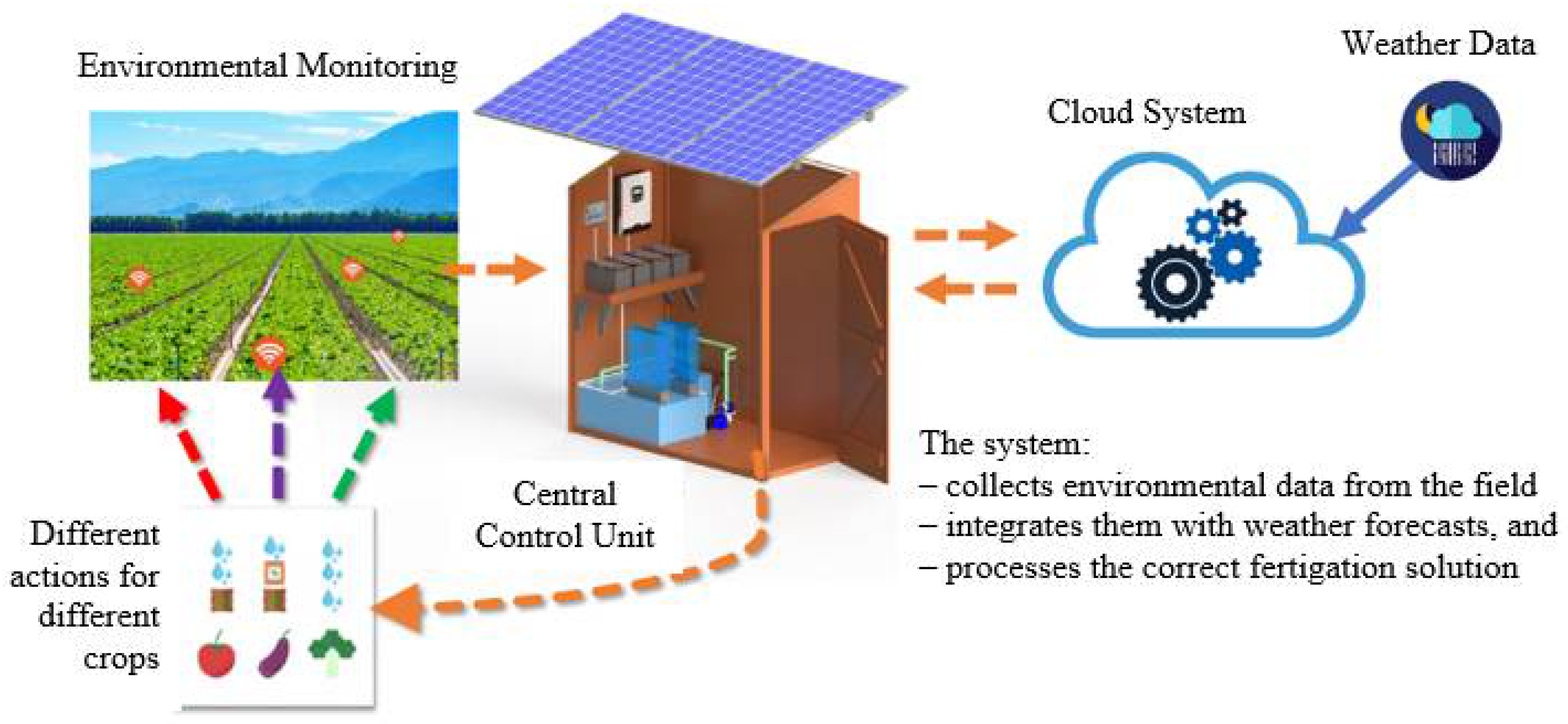
The proposed fertigation system consists of physical modules electrically powered by a photovoltaic power supply and a cloud computing infrastructure for managing the physical modules in an automated way. In fact, despite the informatics infrastructure, it is possible to control and activate the fertigation phases according to the crop type and their growth phase, create a history of operations, and share data by using a tracking system on environmental conditions (Figure 1).

A detailed architecture of the proposed system, sensor node installation, design and management, WSN connection, IoT, data acquisition from sensor nodes, connections and networks, fertigation system, hardware, and software of the fertigation system is described in Visconti et al. [24] and Valecce et al. [25].

2.1. Solar Fertigation Irrigation and Fertilization Agronomic Models

DSS is a major component in charge of making the final decision on the quantity of water to be irrigated, or equivalently, the time to irrigate considering continuous water flow. This decision is considered intelligently on the basis of the information delivered by soil sensors, weather conditions, crop type, and IoT analysis. The aim of this component, therefore, is to operate as a human expert in decision-making processes for the optimization of irrigation and assisting the farmer. The DSS further aims to assure a rational use of fertilizers, water resources, and ultimately a reduced environmental impact. The method allows for integration and optimizes the management of the traditional cropping systems with the current technologies. This estimates the periodicity and fertilizers’ quantity to be provided in the irrigation and fertilization process based on the agronomic methods and collected data for temperature and humidity of both soil and atmosphere. The DSS is integrated with the desktop platform used on several devices, such as personal computers, laptops, mobile phones, or tablets and users can monitor and manage the fertigation activities.

The proposed system is optimized to calculate the amount of water and nutrients needed by the plant. The system calibrates the irrigation scheduling and fertilizer amounts to be used in the irrigation and fertilization phases based on the agronomic models and sensor data.

2.2. Irrigation Scheduling

The daily irrigation amount was estimated starting from the farm, weather and environment, crop and soil data. This involved different factors of technologies to determine irrigation schedules and monitor irrigation and fertilizer applications which further includes the type, rate, time, and amount of fertigation. Thus, the study collected and analyzed the agronomic parameters of precision irrigation strategies with different irrigation schedules and weather conditions.

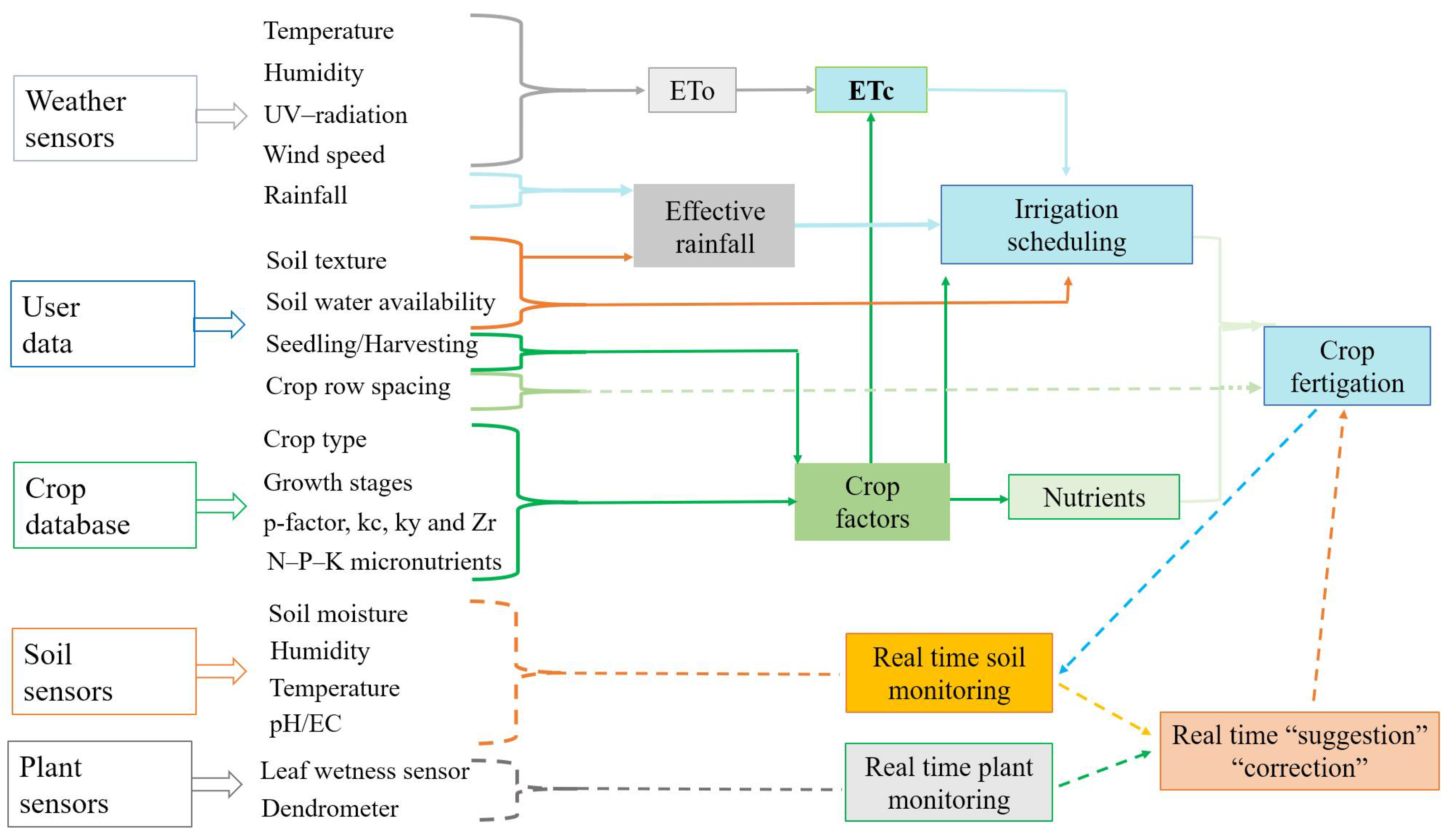
A hybrid system was used for real-time irrigation scheduling (Figure 2). A weather-based method has been integrated with crop data (crop database and user data) and soil data (user data and soil sensors). The agronomic model estimates the ETc, starting from weather data collected by weather sensors and crop factors (kc). The seedling data and crop growth stage were uploaded by the user and/or obtained from databases for detailed crop information. The empirical method that estimates the amount of the effective rainfall consumed by ETo, concerning the utilized rainfall (RU) was adopted. Furthermore, soil texture, crop depletion factor (p), yield factor (ky), and root depth (Zr) were used for the estimation of soil parameters.

2.3. Nutrients

The database reports the accurate amount of the nutrient demands related to the crop growth stage in a form that becomes available in synchrony with crop demands for maximum utilization of nutrients; however, modifications could be performed according to the particular needs of the crop and the farmer. The agronomic database contains precise values related to fertigation needs for each crop type according to the seasonal period and growth phase; based on the agronomic database and WSN data related to soil and environment, the control unit defines the type and optimal quantities of fertilizer, the timing, and the fertigation methods for each crop.

2.4. Real-Time Monitoring and Suggestions

Soil and plant sensors were used by DSS. Soil moisture, humidity, pH, and soil electrical conductivity (EC) were used for real-time monitoring of irrigation and fertigation.

Furthermore, the leaf wetness sensor monitored real-time plant moisture levels in leaves and supported irrigation and water systems. Dendrometer sensors were used for monitoring changes in plant water content (only for fruits).

Real-time monitoring data were used for irrigation and nutrient suggestions and correction strategies.

2.4.1. Irrigation Scheduling

Crop Evapotranspiration (ETc)

ETc is the evapotranspiration from disease-free, well-developed crops, cultivated in open fields, in optimum soil water conditions, and receiving complete production under the provided environmental conditions.

ETc is estimated, using the crop coefficient approach, by multiplying the ETo by a crop coefficient (Kc) [26] which follows as:

ETc = Kc × ETo

(1)

where ETc represents crop evapotranspiration (mm d⁻¹), Kc represents crop coefficient, and ETo represents reference crop evapotranspiration (mm d⁻¹).

ETo is the evapotranspiration rate from a reference surface, not short of water and is one of the major factors for determining optimum irrigation water management. Soil sensors measured the ETo based on soil properties (i.e., soil permittivity, electrical resistance, and soil water potential, among others). The collected ETo values were used for irrigation scheduling at the fields.

Most of the effects of weather parameters are integrated into the ETo equation. Consequently, as ETo is an index of climatic demand, Kc differs predominately with the particular crop features and only to a limited extent with climate. This transfers the standard Kc values between the field and the climate. This has been a major reason for the wide acceptance and beneficial aspects of the crop coefficient approach and the Kc factors analyzed in previous literature [26]. Kc data of the most important crops at different developmental stages were collected in a database according to the FAO manual–56 methods (Section 3.5).

At the present time, the irrigation strategy of the system is based on Hargreaves–Samani (H–S) (Section 3.3); however, the Penman–Monteith (P–M) formula could also be uploaded. Furthermore, an experimental set-up of seven ET crop models is reported in Section 3 and were used for the implementation of the ET equation in the DSS.

The P–M model is recognized as the standard method for ETo assessment which provides the best performance in Mediterranean environments [26,27,28]. However, the need for collecting a relatively large number of parameters (e.g., relative humidity of the air, solar radiation, or wind speed) in different climates, which are generally difficult to estimate with good accuracy, restricts the extensive utilization of this model [28]. Therefore, alternative methodologies requiring lower cost observations have been developed, such as Hargreaves–Samani (H–S), Blaney–Criddle (B–C), Thornthwaite, Priestley–Taylor, Makkink, and Turc, among others [29]. The use of simpler models for ETo estimation with a lower level of parameters could affect accurate irrigation water management, obtaining irrigation schedules of low quality with a bad impact on water savings and crop yield.

The H–S model uses daily maximum and minimum air temperature data as the only input. This empirical model is one of the most commonly used in various studies. It is recommended by Allen et al. [26] as the best estimation model. As an empirical method, H–S involves empirical coefficients. While H–S could be tested with some standard values of these coefficients, several studies [26] recommended testing H–S at locations with comparable weather. ETo values using the H–S depend on the local temperature (Figure 2). Maximum, minimum, and mean temperature and UV-radiation parameters are required. UV-radiation can be estimated for a particular day and location; however, only maximum, minimum, and mean temperature are the parameters that require observation. The H–S method is generally preferred to other more complicated methods since it provides reasonably adequate performance and requires only maximum, minimum, and mean temperatures [30].

Weather parameter data, such as temperature and humidity (DHT22, by Aosong Electronics), UV-radiation (SQ-100 solar radiation sensor, by Apogee Instruments), wind speed, and rainfall were recorded by sensors mounted on the system.

Rainfall (Effective Rainfall)

The rainfall patterns in the local climate significantly affect crop growth and production. The rainwater that is disposed of in the shape of deep percolation or run-off stores in some other resources of the nature and could be utilized in any other usage or part of it is absorbed by the soil which remains stored for a longer time and in a fresh form. The plant’s root zone can easily utilize and uptake the water for its growth, nourishment, and further development. Part of the water content that is utilized by the crops and soil is effective rainfall, which is different in every region of the world depending on its climate, rainfall yearly durations, soil structure and texture, root depth, and variety of planting factors [31].

The proposed system was based on an empirical method that estimates the amount of the effective rainfall consumed by evapotranspiration, with reference to the utilized rainfall (RU), meaning the water content between the wilting point and the field capacity, limited to the layer of soil occupied by the roots [32]. The empirical expression is presented as:

Effective rainfall = fc (1.253 × p^0.824 − 2.935) × 10 [0.001 ET]

(2)

where fc is the correction factor which depends on the usable water stored in the root-zone; p is the total monthly precipitation (mm); and ET is the total monthly evapotranspiration (mm).

Luo et al. [31] reported that estimation and utilization of effective rainfall with DSS could be a significant method to design irrigation saving strategies. Examples of this are validated in Texas, USA [33], Jimma–Ethiopia [34] and Wuhan, China [31].

During the rainfall occurrence, for example for two days, the soil water potential data of the system (soil sensors) recorded similar moisture values continuously for four days (depending on climate). After this, regular irrigation water was provided as per regular schedules.

Crop Factors

The collection of crop factors leads to the development of a crop database for the successful running and efficient management of irrigation. The database illustrates the crop factors, including crop growing stages, stage lengths (days), depletion factor (p), crop coefficient (kc), yield factor (ky), and root depth Zr (Figure 2).

The aforementioned crop data for each crop type was installed into the system. To determine the amount of water applied by the irrigators into the field, during an irrigation event, automatic calibration of the particular growth stage and stage length of the crop were compared with the available humidity at the field.

Frequent readings were taken by the system during these irrigation phases (soil sensors). The system continued the irrigation until the exact values for the p-factor, kc, and ky were reached. When the irrigator completed irrigating the field, the average depth of irrigation water passing through the valves and the respective discharge were read for the measurement of the field being irrigated. The rate of water discharge and the depth of water applied depends on the particular values of the p-factor, kc, and ky, as they differ in every crop type.

Zr of crops depends on the available soil moisture considering compaction levels of the particular soil. Determining the average Zr of each type of crop [26], the soil moisture sensors were installed at a particular soil depth and distance in the fields. The field was irrigated by a couple of irrigators placed at a particular distance from each other. The soil moisture sensors, after reaching the moisture at a particular soil and root depth, sent the information to stop the irrigation promptly.

For irrigation scheduling, the effective Zr of the available crop was considered, irrespective of growth stages. Most of the plant’s roots were located in the upper portion of the root zone; therefore, irrigation scheduling was managed to a shallower depth than the crop’s full root depth. Soil moisture content was estimated two times; one on a daily basis and one before each irrigation application during the field experiments. Using the soil moisture data acquired by the system (soil sensors), the depletion factor (p) of available soil water in the provided crop zr was estimated by the equation [35]:

p-factor = 1001n∑1nFC_i − θ_iFC_i − WP

(3)

where n is the number of layers of the rooting depth (zr), FC_i is the soil moisture at field capacity, θ_i is the soil moisture in the ith layer, and WP is the soil moisture at permanent wilting point.

The system can implement the database with data collected through the installation of plant-based sensors that replace table data with real time data.

Although less precise, the use of a database allows users to easily manage all the parameters which were considered useful for optimum irrigation management.

Soil Water Availability

Soil water availability is the capacity of soil to collect water available to crops. After irrigation, the soil drains until the field capacity. Field capacity is the amount of water that soil should preserve at a particular volume. In the absence of a water supply, the water level in the root zone decreases after uptake by the crop. As water uptake continues, the available water is tightly held by the soil particles, and makes it harder for the plant to extract it. Ultimately, a point is reached where the plant can no longer extract the available moisture. This makes the water uptake zero and leads to the wilting point. Wilting point is the water content at which plants start to permanently wilt and is a factor function of the soil texture. The total amount of water that can be stored in the root zone is a function of the type of soil texture [26].

As the water content more higher than field capacity cannot be held and as the water content lower than wilting point cannot be extracted by plants, the total available water (TAW) in the root zone is the difference between water content at field capacity and wilting point [26] such as:

TAW = (θ_FC − θ_WC) × Zr

(4)

where TAW represents total available water in the root zone (mm), θ_FC represents water content at field capacity (m³ m⁻³), θ_WP represents water content at wilting point (m³ m⁻³), and Zr represents root depth (m).

Though water is available until the wilting point, crop water extraction is minimized well before the wilting point. In the wet soil, the soil quickly supplies enough water to meet the crop demands. However, upon the reduction in the soil water content, water becomes tightly bound to the soil matrix and is more difficult to utilize. When the soil water content reduces below a particular threshold, soil water can no longer be transported to the roots to complete the transpiration demand, ultimately, the crop starts to stress. The fraction of TAW that a crop can utilize without experiencing stress is called readily available water (RAW) [26] such as:

RAW = p × TAW

(5)

where RAW is the readily available water in the root zone (mm); and p is the average fraction of TAW (0–1).

According to soil type, cultivated crop, and root depth the RAW and TAW data were calculated and uploaded to the irrigation system.

2.4.2. Nutrients

Nutrient management was supported by the proposed system and easily used for fertigation, through which crop nutrient requirements were met accurately. Due to the method the water is applied by the system, surface applications of nutrients are sometimes ineffective, so the system automatically mixed liquid nutrients with the irrigation water.

The system allowed the delivery of nutrients and water (fertigation) to plants in accurate quantities and at the appropriate time for a particular stage of plant growth. The major factor in the fertigation process was the time, and the key in the application was striking the correct balance for optimal plant life with optimal use of water. The system also performed the fertigation application in which the fertigation was based on the relevant amounts of water and nutrients that must be given periodically, with no feedback. Meanwhile, the second type was based on a combination of fertigation application and feedback of the necessary data to determine the amount of fertigation needed [36,37].

The database reports the accurate amount of the nutrient demands related to the crop growth stage in a form that becomes available in synchrony with crop demands for maximum utilization of nutrients; however, modifications could be performed according to the particular needs of the crop and the farmer.

The control unit compares received information with those stored in the database; thus defining the type and concentrations of the fertilizers and regulating the timing of the irrigation. These operations are obtained properly by driving the different hydraulic/mechanical sections for adjusting fertilizer quantities to be introduced into the aqueous solution in the bin. Furthermore, the control unit drives the electric pump and solenoid valves, for correctly distributing the fertilizing solution into the different areas of the land; in fact, the system is designed in a modular way according to the extension of the land to cultivate. The definition of agronomic mathematical models is fundamental for processing data collected by the WSN and comparing them with those reported in the database to create a dynamic system for optimal fertigation control. The agronomic database contains precise values related to fertigation needs for each crop type according to the seasonal period and growth phase; based on the agronomic database and WSN data related to soil and environment, the control unit defines the type and optimal quantities of fertilizer, the timing and the fertigation methods for each crop kind, with the purpose to optimize water use and improve the quality and quantity of cultivated products.

Crop Database

A database for nutrients and irrigation management of nine crops was developed; furthermore, a study for other crops is in progress (

Table 1. Crop database of different crops and their important parameters.

Crops/Parameters	p-Factor	Temperature Requirement (°C)	Root Depth (Zr) (m)	Crop Coefficient (kc)	Yield Factor (ky)	Fertilizers (N-P-K) (kg ha−1)	Crop Water Requirement (mm Growing Season−1)	References
Citrus (Citrus sinensis and Citrus limon	0.5	23–30	1.2	0.70	0.8–1.1	100-35-50	900–1200	[38]
Olive (Olea europaea)	0.65	15–25	6.0	0.70	0.2	200-55-160	600–800	[39]
Soybean (Glycine max)	0.5–0.9	18–35	1.0	1.15	0.2–1.0	20:40:20	450–700	[40]
Potato (Solanum tuberosum)	0.9	18–20	1.0	0.5	0.85	34-0-0	500–700	[41]
Cabbage (Brassica oleracea var. capitata)	0.4	20–25	0.5	0.95	0.60	45:45:45	380–500	[40]
Onion (Allium cepa)	0.3	20–30	0.6	0.75	0.3	60-25-45	350–550	[39]
Pepper (Capsicum annuum)	0.3	18–27	0.8	0.9	1.1	5-10-10	600–1250	[42]
Tomato (Lycopersicon esculentum)	0.3	18–25	1.0	0.9	0.4	200:250:250	400–600	[42]
Watermelon (Citrullus lanatus)	0.4	21–29	0.8	0.75	0.3	80-25-35	600–800	[1,43]

).

2.4.3. Sensors for Real-Time Soil Moisture and Plant Water Content Monitoring

Soil sensors are specific devices that convert a physical parameter into soft data. The soil sensors are used to collect and communicate the parameters, such as soil moisture, humidity, and temperature (Figure 2). For estimating the particular water level, sensors were connected to the main irrigation canals, while for estimating the water flow, they were connected to a water pump. Sensors were further connected to the database which was periodically sending the data. The connected database was monitoring the irrigation water levels, analyzed the data stored, and compared it with the threshold values. The threshold values of soil moisture were uploaded into the database to maintain the irrigation on a daily basis. Using threshold values, the system started or stopped the irrigation based on the moisture content of the soil. In this way, soil sensors controlled the flow rate of water from the tank to the irrigation field and optimized the use of water. Soil sensors significantly supported water management decisions, used for continuously monitoring water levels in the tank and moisture in the soil and provided an accurate amount of water required for crop plants. The sensors checked the temperature and humidity of soil to retain the nutrient composition of the soil managed for the growth of crops.

Soil sensors efficiently schedule the irrigation events by either decreasing or increasing the intensity/frequency of water, preserving the important soil nutrients, and on the other side, providing a thirst factor to plants at their particular stage of growth. Soil sensors empower the farmers to manage the water levels without any requirement for a physical presence in the field. They correctly measure the accurate level of soil moisture and aid in scheduling the irrigation supply and distribution in an efficient method. They significantly help in fertigation and irrigation management by analyzing the soil parameters affecting crop growth and production (Figure 2).

The types of sensors used in the smart irrigation system are real-time fertigation monitoring sensors for environmental and soil parameters. The sensor nodes are isomorphic and non-rechargeable with the initial energy being the same as E₀.

MQTT is an extremely simple and lightweight messaging protocol, designed for constrained devices and low-bandwidth, high-latency, or unreliable networks. All content is delivered to the user interface using an MQTT protocol and ActiveMQ message broker deployed on AWS as software as a service [25].

For real-time fertigation monitoring, several sensors, such as DHT22, SHT11, SEN0193, and SEN0193 acquired environmental and soil parameters during the study period [24]. Plant sensors such as leaf wetness and dendrometer sensor data could be uploaded. Furthermore, data recorded onsite included the irrigation water pH and EC for water quality information. The samples were checked for a pH of less than 2. The irrigation water was then checked for microbial activities and undesirable physicochemical reactions before further analysis.

The leaf wetness sensor, such as the radio frequency identification (RFID) sensor [44], monitored real-time plant moisture levels in leaves and supported irrigation and water systems. The dendrometer sensors, such as ZN12-O-WP [45] (only for fruits), were used for detailed crop information. ZN12 measures microvariations in stem diameter caused by cycles of shrinking and swelling, which indicate changes in plant water content.

Similar to soil sensors, the threshold values for leaf water content were also uploaded into the database to manage the irrigation on a daily basis.

2.4.4. Web-Based Platform

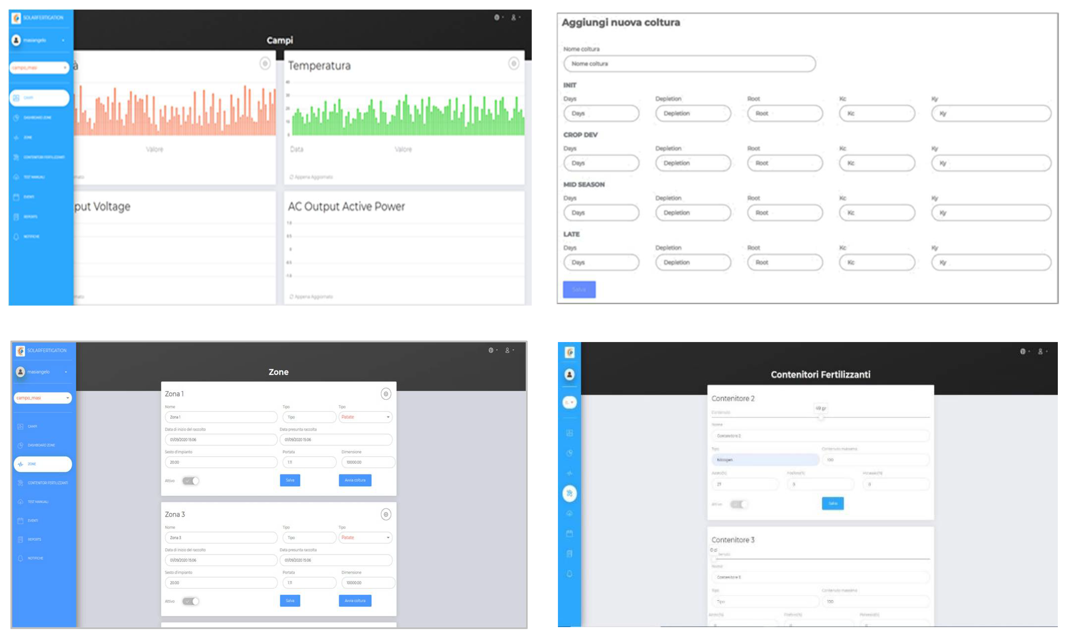
The web-based platform is a highly efficient irrigation management system. The platform monitors seven different categories, including all fields, zones, the containers of the fertilizer, manual tests, events, reports, and notifications. After receiving the initial data from the field, the platform manages, processes, analyzes, and finally, displays the data in a simple and user-friendly way. The display factors include fields, crops, environmental conditions, irrigation hours, soil humidity, fertilizer amount, and their problems to solve. While, the displayed crop factors are crop growing stages, stage lengths (days), depletion factor (p), crop coefficient (kc), yield factor (ky) and root depth (Zr), as shown in Figure 3. It also displays suggestions in a timely manner so that they could be addressed without having a higher amount of irrigation or damaging the crop. All the information and data analysis could be performed using the computer and mobile. The platform shows an energy-efficient method to increase the system’s lifetime and reduce the project’s cost.

Moreover, the installation of the smart fertigation system using the crop sensors, only collects the soil moisture content but not the water depth. However, water depth is a vital factor for understanding the ETo, growth, and development of the crops [46]. The ETo calculation must be conducted on a daily basis with high precision, which is dependent on the environmental factors of the tested fields and the methodology.

The summary of the most important factors of solar fertigation is described as: (a) Describing different fields and the particular crop and weather information. It also shows the power voltage and active power of the system; (b) shows different crops and their particular parameters during their different growth stages and stage lengths; (c) presents different zones of fertigation of crops, seedling and harvest data, types, and row spacings. It also shows the activation and deactivation of the fertigation in that particular zone of the field; (d) shows the level and quantity of fertilizers in a container; (e) irrigation and fertilization schedules; (f) solar fertigation remote application through which farmers could monitor and control the fertigation in different fields.

3. The Proposed System: Experimental Setup for ET Crop Models

The study consists of different regions in which the range of fields were estimated from 10 to 12 hectares. The field sensors collected soil and weather data after every 30 min, such as temperature (°C), relative humidity (%), solar radiation (MJ m⁻²), air speed (km h⁻¹), rainfall (mm), and soil humidity. This data is considered solar fertigation system data. One weather sensor was deployed in each experimental field. The number of soil sensors range from 3 to 9 in each field (3 for each sector), respectively, with three different depths starting from 10 to 50 cm; however, they were installed into the positions where the WSN network could be developed in all parts of the field. Moreover, real-time API weather data was also connected to the DSS for data collection using the web-based resources which are considered as API data. The experimental setup analyzed the comparison of both, solar fertigation and API data with the standard combination-based FAO P–M model [26] on the basis of statistical attributes using six different empirical models. Those are three temperature-based models, such as Hargreaves–Samani (H–S) [47], Blaney–Criddle (B–C) [48], and Thornthwaite [49]; and three radiation-based models, such as Priestley–Taylor [50], Makkink [51], and Turc [52]. This study will further contribute to understanding the accuracy and acceptable efficiency of each model for estimating ETo in the Mediterranean region of Italy. Daily meteorological data from seven weather stations for the period 1 January 2019–31 December 2021 were considered.

3.1. Study Area

The study was performed in Molise and Apulia regions of Italy. The four weather stations of Molise region were W1–Campobasso, W2–Ferrazzano, W3–Oratino, and W4–Ripalimosani (

Table 2. Details of the weather stations where tests were conducted.

S. No.	Weather Stations	Altitude (m a.s.l.)	Time Period of Tests
	Molise Region
1.	W1–Campobasso	700	1 January 2019–31 December 2021
2.	W2–Ferrazzano	900	1 January 2019–31 December 2021
3.	W3–Oratino	795	1 January 2019–31 December 2021
4.	W4–Ripalimosani	640	1 January 2019–31 December 2021
	Apulia Region
5.	W1–Montemesola	183	1 January 2019–31 December 2021
6.	W2–Castellaneta	5	1 January 2019–31 December 2021
7.	W3–Marina di Ginosa	12	1 January 2019–31 December 2021

). The region is situated in a non-homogeneous mountainous zone. The climate is Mediterranean type, which further consists of an annual average temperature of 13.2 °C, with the monthly averages of 4.6 and 22.8 °C in January and August, respectively; the lowest average temperature is 2.1 °C in January while the highest average temperature is 35 °C in July. The average annual rainfall is 820 mm, divided over 82 days, within 2 months of slight summer. A historical trend in the decreased rate of rainfall is highlighted, mostly in the summer season; this climate change is defining an uprise in the Mediterranean climate in this particular region.

Furthermore, three weather stations in the Apulia region were W1–Montemesola, W2–Castellaneta, and W3–Marina di Ginosa (Table 2). The region is known for its Mediterranean-type climate with short and mild winters, and hot, long, and dry summers [53].

The data were collected on a daily basis while a precise quality control check for the ETo variables was performed. This guarantees the data homogeneity and addresses any error.

3.2. Data Collection

Data from seven weather stations in different Mediterranean zones of Italy were collected from solar fertigation systems (soil sensors) and API (MeteoInMolise–http://www.meteoinmolise.com/ (5 January 2022)). The collected crop data includes crop water requirement, fertilizer requirement, stages of development, stage length (in days), depletion coefficient (p), root depth (Zr), crop coefficient (kc), and yield response factor (ky). The collected meteorological data includes minimum, maximum, and average temperatures; minimum, maximum, and average humidity; UV-radiation; minimum, maximum, and average atmospheric pressure; actual airspeed; and rainfall. The data was then managed by a web-based desktop platform for further processes.

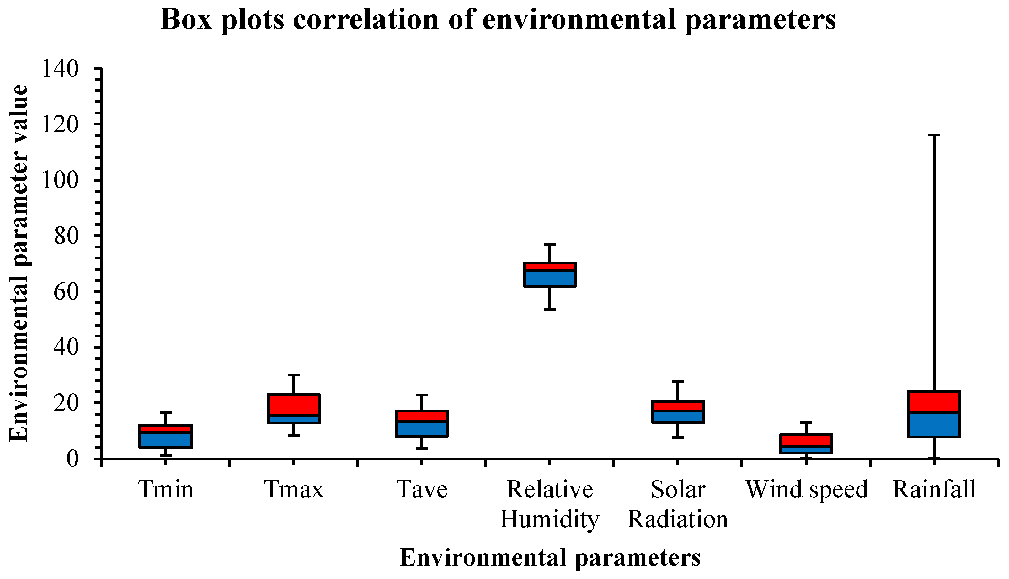
The mean correlation of monthly temperatures and rainfall at seven weather stations for the study period was recorded. Minimum and maximum temperature and rainfall were recorded on a monthly basis for each weather station. A box plot correlation of environmental parameters, such as minimum and maximum temperature, minimum and maximum relative humidity, solar radiation, and daily wind speed for three years of data were tested in the study (Appendix A,

Table A1. Mean collected environmental parameters used for daily ETo estimation at Molise region from 1 January 2019 to 31 December 2021.

Months	Minimum Temperature (°C)	Maximum Temperature (°C)	Average Temperature (°C)	Relative Humidity (%)	Solar Radiation (MJ m−2)	Air Speed (km h−1)	Rainfall (mm)
19 January	0.21	4.07	2.14	72.84	10.74	1.07	80.20
19 February	1.70	8.57	5.13	67.08	16.00	6.23	46.33
19 March	4.37	13.36	8.86	62.13	18.64	0.75	31.88
19 April	6.57	14.84	10.70	61.34	26.16	1.11	65.38
19 May	7.85	15.39	11.62	66.13	25.68	2.93	153.45
19 June	17.60	28.09	22.84	67.94	24.35	10.35	17.55
19 July	18.11	28.83	23.47	60.82	16.46	9.22	31.88
19 August	18.55	30.59	24.57	71.73	18.73	10.40	28.53
19 September	14.34	23.56	18.95	76.74	17.74	6.43	41.20
19 October	11.30	20.22	15.76	56.71	19.73	2.81	40.33
19 November	7.62	13.50	10.56	69.78	11.15	5.27	135.18
19 December	3.91	9.54	6.72	71.63	10.45	1.84	79.78
20 January	2.35	9.54	5.95	73.83	11.73	2.55	3.05
20 February	3.31	11.85	7.58	68.07	16.99	7.71	23.38
20 March	3.64	11.77	7.70	63.12	19.63	2.23	94.90
20 April	6.85	15.96	11.41	62.33	27.15	2.59	29.13
20 May	11.23	20.55	15.89	67.12	26.67	4.41	57.03
20 June	13.87	23.47	18.67	68.93	25.34	11.83	60.05
20 July	17.02	27.98	22.50	61.81	17.45	10.70	37.46
20 August	18.38	29.60	23.99	70.67	17.67	9.83	64.20
20 September	14.09	24.56	19.33	75.68	16.68	5.86	65.68
20 October	9.11	17.54	13.33	55.65	18.67	2.24	31.31
20 November	6.63	13.72	10.17	68.72	10.09	4.70	70.93
20 December	3.81	9.82	6.81	70.57	9.39	1.27	125.28
21 January	1.31	6.93	4.12	70.74	8.76	1.38	113.75
21 February	3.86	12.12	7.99	64.98	14.02	6.54	39.78
21 March	2.64	10.50	6.57	60.03	16.66	1.06	54.65
21 April	5.00	13.81	9.40	59.24	24.18	1.42	27.13
21 May	10.84	20.55	15.69	64.03	23.70	3.24	34.83
21 June	16.50	27.33	21.92	65.84	22.37	10.66	26.60
21 July	18.86	29.98	24.42	58.72	14.48	9.53	28.35
21 August	18.19	29.71	23.95	69.62	16.75	10.71	25.28
21 September	14.56	24.54	19.55	74.63	15.76	6.74	28.45
21 October	8.83	15.58	12.20	54.60	17.75	3.12	9.15
21 November	7.95	12.49	10.22	67.67	9.17	5.58	209.98
21 December	3.56	9.14	6.35	69.52	8.47	2.15	105.10

and

Table A2. Mean collected environmental parameters used for daily ETo estimation at Apulia region from 1 January 2019 to 31 December 2021.

Months	Minimum Temperature (°C)	Maximum Temperature (°C)	Average Temperature (°C)	Relative Humidity (%)	Solar Radiation (MJ m−2)	Air Speed (km h−1)	Rainfall (mm)
19 January	3.09	10.09	6.59	76.31	17.43	6.48	66.83
19 February	5.24	13.25	9.25	70.55	22.69	11.64	22.77
19 March	7.64	16.74	12.19	65.60	25.33	6.16	22.33
19 April	10.23	18.73	14.48	64.81	32.85	6.52	19.40
19 May	11.74	20.40	16.07	69.60	32.37	8.34	10.10
19 June	19.24	31.71	25.48	71.41	31.04	15.76	8.00
19 July	20.46	32.81	26.64	64.29	23.15	14.63	6.50
19 August	21.46	34.54	28.00	75.20	25.42	15.81	8.40
19 September	18.52	28.27	23.40	80.21	24.43	11.84	21.57
19 October	14.10	24.27	19.19	60.18	26.42	8.22	24.33
19 November	11.27	18.87	15.07	73.25	17.84	10.68	36.93
19 December	7.76	14.41	11.09	75.10	17.14	7.25	52.60
20 January	5.16	13.71	9.43	77.45	18.57	7.62	21.97
20 February	6.26	15.06	10.66	71.69	23.83	12.78	7.10
20 March	6.99	15.48	11.23	66.74	26.47	7.30	7.87
20 April	9.25	18.28	13.77	65.95	33.99	7.66	8.83
20 May	13.72	23.21	18.47	70.74	33.51	9.48	9.47
20 June	16.95	26.56	21.76	72.55	32.18	16.90	12.00
20 July	20.37	31.18	25.78	65.43	24.29	15.77	11.47
20 August	21.74	32.10	26.92	74.29	24.51	14.90	9.23
20 September	18.92	28.38	23.65	79.30	23.52	10.93	18.67
20 October	12.42	21.63	17.03	59.27	25.51	7.31	38.53
20 November	10.21	17.73	13.97	72.34	16.93	9.77	65.37
20 December	7.21	14.30	10.76	74.19	16.23	6.34	81.10
21 January	4.73	12.03	8.38	74.83	16.07	7.41	68.77
21 February	6.43	14.23	10.33	69.07	21.33	12.57	40.77
21 March	5.73	14.24	9.98	64.12	23.97	7.09	31.50
21 April	8.23	16.45	12.34	63.33	31.49	7.45	15.83
21 May	13.27	23.75	18.51	68.12	31.01	9.27	5.90
21 June	18.98	29.90	24.44	69.93	29.68	16.69	4.63
21 July	21.86	32.63	27.25	62.81	21.79	15.56	5.77
21 August	22.06	32.27	27.16	73.71	24.06	16.74	4.67
21 September	17.85	27.04	22.44	78.72	23.07	12.77	32.40
21 October	12.88	20.38	16.63	58.69	25.06	9.15	52.87
21 November	12.12	17.57	14.84	71.76	16.48	11.61	105.13
21 December	8.06	14.86	11.46	73.61	15.78	8.18	96.70

; Figure A1 and Figure A2).

Mean collected parameters, such as maximum, minimum, and average temperature, relative humidity, solar radiation, airspeed, and rainfall for the study period (1 January 2019–31 December 2021) were acquired. In addition, temperature and rainfall trends were recorded as linear. However, MAE, MSE, RMSE, and R statistical attributes were tested for the following temperature-, radiation-, and combination-based models.

3.3. Temperature-Based Models

3.3.1. Hargreaves–Samani (H–S) Model

The lack of available agrometeorological data (such as solar radiation, air humidity, and wind speed) in all climatic regions limits the use of the standard FAO P–M model [26]. Therefore, Allen et al. [26] proposed the application of the H–S model in particular regions where only the data related to air temperature is available. The Hargreaves–Samani (H–S) model [47] is an empirical approach that needs theoretical parameters for ETo estimation. The model is expressed as follows:

ETo = 0.023 (0.408) (T_mean + 17.8) (T_max − T_min)^0.5 × R_a

(6)

where ETo represents reference evapotranspiration (mm d⁻¹); Ra represents extraterrestrial radiation (MJ m⁻² d⁻¹); T_mean represents average monthly/annual temperature; and T_max and T_min are daily maximum and minimum air temperatures (°C), respectively.

3.3.2. Blaney–Criddle (B–C) Model

The Blaney–Criddle (B–C) model [54] is recommended for the daily estimation of ETo (mm d⁻¹). The equation is expressed as follows:

ETo = p (0.46T_mean + 8.13)

(7)

where ETo represents daily reference evapotranspiration (mm d⁻¹) and T_mean represents daily mean temperature (°C). In our study, T_mean is measured based on daily T_max and T_min (such as T_mean = (T_max + T_min)/2). The coefficient p is considered as the daily percent of annual daytime hours for each day of the year, which may be estimated using the latitude and the Julian day analysis [26].

3.3.3. Thornthwaite Model

Thornthwaite [49] proposed an empirical model to estimate ETo by comparing the correlation between temperature, precipitation, and changing rate of water in diverse regions. This required only readily available input data for estimating ETo. This is based only on daily averaged temperatures and latitude, the latter variable used to calculate the maximum amount of sunshine duration [55]. The equation is expressed as follows:

ETo = 16N_m [(10T_m)^a1]

(8)

where T_m represents mean air temperature (°C), N_m represents the number of days in a month, and al represents the average number of daylight hours per day for each month.

3.4. Radiation-Based Models

3.4.1. Priestley–Taylor Model

The Priestley–Taylor [50] model is tested in a diverse range of regions for ETo estimation. The model was initially developed for saturated environments and open water bodies with low wind effects. The wind factor multiplied by vapor pressure deficit was further simplified and joined with land cover and site condition data. ETo estimation using this model has provided some good results, depending on the region. The Priestley–Taylor method requires only temperature and radiation data and is considered as precise among the simplified methods with reduced parameters [56]. The method includes a correction factor known as the advection coefficient with the value of 1.26 [50] and ranging between 1.08 and 1.34 for agricultural fields [56]. The model is expressed as follows:

$$\mathrm{ETo}=1.26\frac{\Delta }{\Delta + \mathsf{\gamma }}\left({\mathrm{R}}_{\mathrm{n}}-\mathrm{G}\right)\frac{1}{\mathsf{\lambda }}$$

(9)

where R_n represents net radiation of the crop surface (MJ m⁻² day⁻¹); Δ represents the slope vapor curve (kPa °C⁻¹); λ represents the latent heat of vapor (MJ kg⁻¹); G represents the soil heat flux density (MJ m⁻² day⁻¹); and γ represents the psychrometric constant (kPa °C⁻¹).

3.4.2. Makkink Model

The Makkink [51] model is also considered a reliable and easy method for the estimation of ETo. Solar radiation is the only required parameter as input data for estimating ETo, which in most areas of the world is easily acquired. The equation is expressed as follows [51]:

$$\mathrm{ETo}=0.61\times \frac{\Delta }{\left(\Delta +\mathsf{\gamma }\right)}\times {\mathrm{R}}_{\mathrm{s}}-0.12$$

(10)

where R_s represents solar radiation (MJ m⁻² day⁻¹); γ represents the psychrometric constant (kPa °C⁻¹); and Δ represents the slope vapor curve (kPa °C⁻¹).

3.4.3. Turc Model

The Turc [52] model provides good data in a diverse set of environmental conditions. It is considered one of the simplest and accurate empirical equations used to estimate ETo under humid conditions. The Turc model requires minimum weather parameters such as mean daily values of temperature and solar radiation (Rs) [57]. The equation is expressed as follows:

$$\mathrm{ETo}=\frac{{\mathrm{T}}_{\mathrm{mean}}}{{\mathrm{T}}_{\mathrm{mean}}+15}\left({\mathrm{R}}_{\mathrm{s}}\times 23.8846+50\right)$$

(11)

where T_mean represents daily mean temperature (°C); and R_s represents solar radiation (MJ m⁻² day⁻¹).

3.5. Combination-Based Model

Standard FAO Penman–Monteith (P–M) Model

ETo is described as the simultaneous loss of water from vegetation and soil surfaces. The quantity of ETo depends on the presence of water at the surface, the quantity of available energy (to convert the phase of water: latent heat of evaporation, LE), the ability of an environment to accommodate water vapor (vapor pressure deficit, VPD), and the procedure for water transport from the soil surface to the atmosphere (turbulent transport). Net radiation (R_n) is the primary source of energy, and wind-generated turbulence is considered the transport process.

ETo is considered as a hypothetical reference crop with particular characteristics, such as a well-watered, 0.12 m grass with an albedo of 0.23, and an aerodynamic surface resistance of 70 s m⁻¹. The equation is expressed as follows:

$$\mathrm{ETo}=\frac{0.408\Delta \left({\mathrm{R}}_{\mathrm{n}}-\mathrm{G}\right)+ \mathsf{\gamma }\frac{900}{\mathrm{T}+273}\mathrm{U}2\left({\mathrm{e}}_{\mathrm{s}} - {\mathrm{e}}_{\mathrm{a}}\right)}{\Delta + \mathsf{\gamma } \left(1+0.34 \mathrm{U}2\right)}$$

(12)

where Δ is the slope of saturation vapor pressure at temperature curve (kPa K⁻¹); R_n is net radiation at the crop surface (MJ m⁻² day⁻¹); G is soil heat flux density (MJ m⁻² day⁻¹); γ is the psychrometric constant (kPa K⁻¹); U2 is the wind speed at 2 m above surface height (m s⁻¹); e_s is the saturation vapor pressure (kPa); e_a is the actual vapor pressure (kPa); (e_s − e_a) is the saturation vapor pressure deficit (kPa); and T is the mean daily air temperature at 2 m height (°C).

3.6. Data Analysis

Data analyses were performed to validate the precision of the proposed system and API results. The statistical parameters such as mean absolute error (MAE), mean square error (MSE), root mean square error (RMSE), and Pearson correlation coefficient (R) for each empirical model were studied to evaluate their effectiveness [58]. The MAE estimates the average magnitude of errors without considering their sign and test samples of absolute differences between the observed (system) and the estimated (API) data (Equation (12)). MSE is an average of squared differences between the observed (system) and the estimated (API) data or is the variance of an error (Equation (13)). RMSE is the square root of MSE or is the standard deviation of an error (Equation (14)). R shows the correlation with a direct and inverse relationship between the observed (system) and the estimated (API) data (Equation (15)). Statistical correlation of temperature-based models (H–S, B–C and Thornthwaite), and radiation-based models (Priestley–Taylor, Makkink and Turc) were compared with the standard FAO P–M model [26] to understand the accuracy and acceptable efficiency of each model [59]. The statistical parameters evaluated are as follows:

$$\mathrm{Mean} \mathrm{absolute} \mathrm{error} \left(\mathrm{MAE}\right)=\frac{{\sum }_{i=1}^n\left|x_i-y_i\right|}{n}$$

(13)

$$\mathrm{Mean} \mathrm{square} \mathrm{error} \left(\mathrm{MSE}\right)=\frac{1}{n}{\sum }_{i=1}^n\left(y_i-{\hat{y}}_i\right)2$$

(14)

$$\mathrm{Root} \mathrm{mean} \mathrm{square} \mathrm{error} \left(\mathrm{RMSE}\right)=\frac{\sqrt{{\sum }_{i=1}^n\left(x_i-y_i\right)2}}{n}$$

(15)

$$\mathrm{Pearson} \mathrm{correlation} \mathrm{coefficient} \left(\mathrm{P}\right)=\frac{{\sum }_{i=1}^n\left(x_i-\overline{x}\right)(y_i-\overline{y})}{\sqrt{{\sum }_{i=1}^n\left(x_i-\overline{x}\right)2(y_i-\overline{y})2}}$$

(16)

where x_i is the forecasted data of temperature, y_i is an observed (system) data of temperature, ŷ_i is the forecasted data, i is the forecasted parameter sequence number (such as 1, 2, 3, 4, and so on), $\overline{x}$ is mean forecasted data of parameter sequence number, $\overline{y}$ is mean observed (system) data of parameter sequence number, and n is the number of the forecasted data.

4. Results

Results were collected from meteorological data which include minimum, maximum, and average temperatures; minimum, maximum and average humidity; UV-radiation; minimum, maximum, and average atmospheric pressure; actual air speed; and rainfall during the study period from 1 January 2019 to 31 December 2021. Environmental parameters, such as temperature, RH, and wind speed range from T_min = 0.21–18.86 °C, T_max = 4.07–30.6 °C, RH = 54.6 –76.7%, and wind speed = 0.75–11.8 km h⁻¹ in Molise (Appendix A, Table A1); while 3.09–22.1 °C, T_max = 10.1–34.5 °C, RH = 58.7–80.2%, and wind speed = 6.16–16.90 km h⁻¹ in Apulia regions, respectively (Appendix A, Table A2).

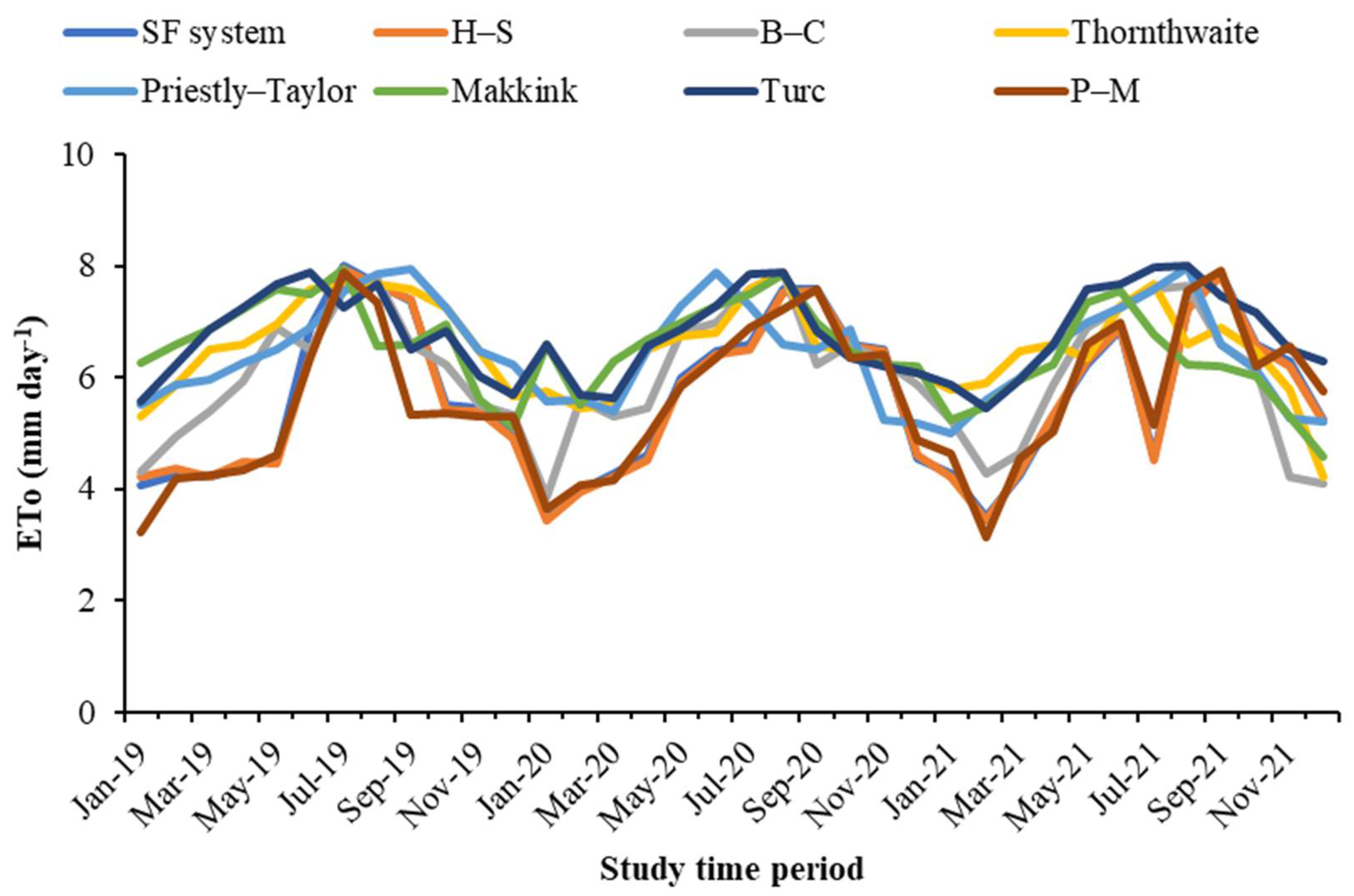
The mean ETo data were analyzed by six different (three temperature- and three radiation-based) methods and compared with the standard combination-based FAO P–M method. Results showed that maximum values of solar fertigation ETo were recorded in the summer months followed by spring and winter. Meanwhile, total ETo for the solar fertigation system, H–S, and P–M was revealed as 3032.8, 3049.9, and 2967.3 mm in Molise, respectively; while 5362.8, 5384.3, and 5422.2 mm in Apulia, respectively, from 1 January 2019 to 31 December 2021.

The estimated monthly and total ETo for solar fertigation system, temperature- and radiation-based models were collected. A significant correlation for the data between the system and the standard FAO model was revealed upon their comparison. The combination-based standard FAO P–M revealed a close trend to the solar fertigation system with no underestimation. The H–S for total ETo shows a highly significant correlation with the standard FAO P–M. While, B–C and Thornthwaite models overestimated the considerable value. Similarly, the monthly and annual estimation of ETo in radiation-based (Priestley–Taylor, Makkink and Turc) models were acquired. Their correlation recorded the highest overestimation from the standard FAO model.

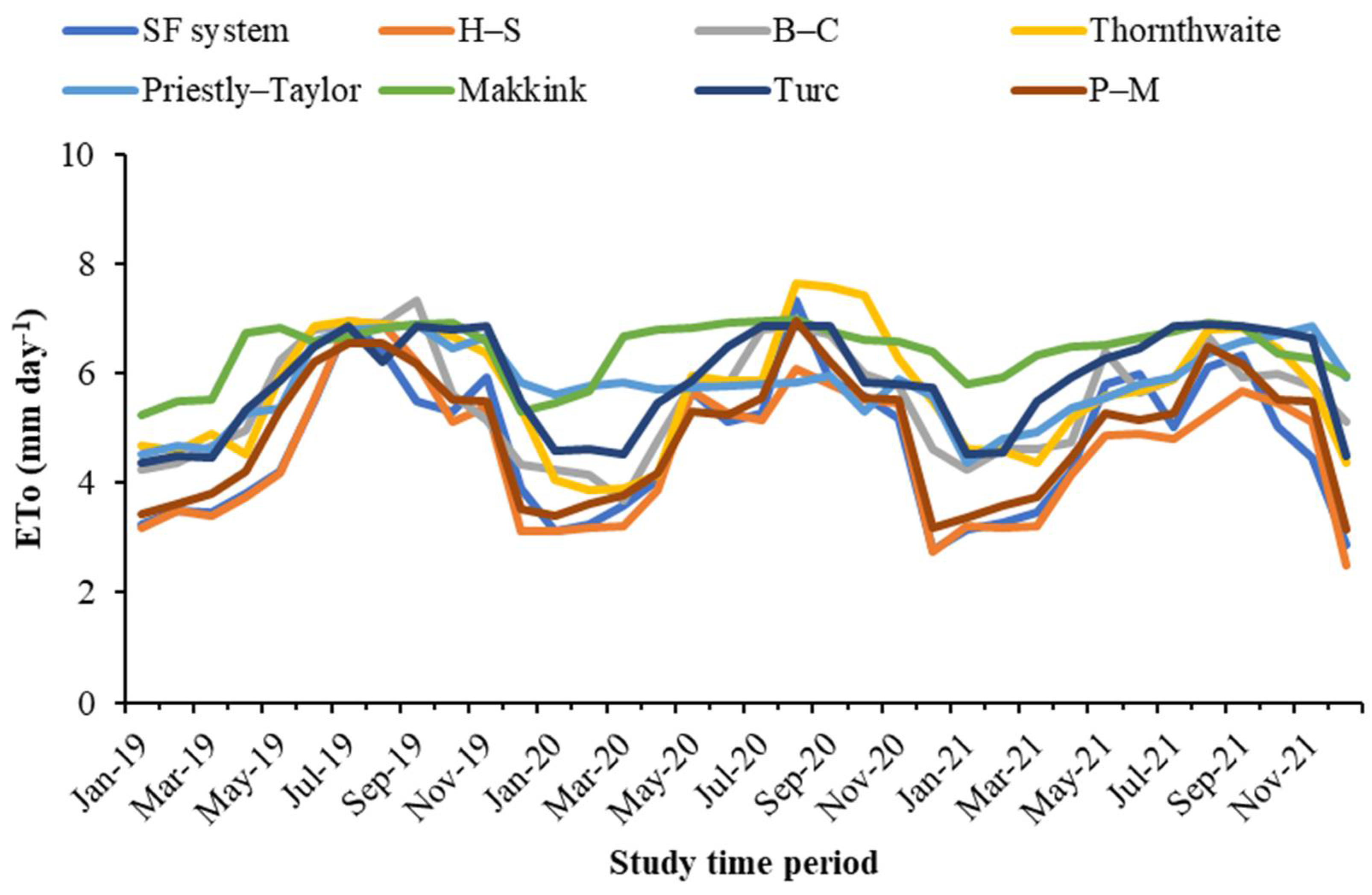
Furthermore, daily ETo in Molise and Apulia regions are displayed in Figure 4 and Figure 5, respectively, for the study period (1 January 2019–31 December 2021). The tested models (B–C, Thornthwaite, Priestley–Taylor, Makkink and Turc) overestimated the ETo compared to the standard FAO P–M [30,60,61,62]. Meanwhile, solar fertigation system values slightly underestimated the ETo. However, both the system and H–S models showed a very close correlation to the standard FAO P–M.

MAE, MSE, RMSE, and R statistical attributes resulted from three temperature-based (H–S, B–C, and Thornthwaite), and three radiation-based (Priestley–Taylor, Makkink, and Turc) models were compared to the standard combination-based FAO P–M [26] during the study period from 1 January 2019 to 31 December 2021 as shown in

Table 3. Mean statistical attributes estimated by temperature- and radiation-based models compared with the standard combination-based FAO P–M model in Molise region over the study period from 1 January 2019 to 31 December 2021.

Statistical Attributes/Models	Mean Absolute Error (MAE)	Mean Square Error (MSE)	Root Mean Square Error (RMSE)	Pearson Correlation Coefficient (R)
Solar fertigation system	0.52	0.63	0.93	0.84
H–S	0.55	0.62	0.97	0.87
B–C	0.67	0.84	1.14	0.97
Thornthwaite	0.75	0.95	1.29	1.16
Priestley–Taylor	0.87	1.09	1.31	1.22
Makkink	0.95	1.36	1.74	1.65
Turc	0.83	1.17	1.45	1.57

and

Table 4. Mean statistical attributes estimated by temperature- and radiation-based models compared with the standard combination-based FAO P–M model in Apulia region over the study period from 1 January 2019 to 31 December 2021.

Statistical Attributes/Models	Mean Absolute Error (MAE)	Mean Square Error (MSE)	Root Mean Square Error (RMSE)	Pearson Correlation Coefficient (R)
Solar fertigation system	0.63	0.72	0.92	0.84
H–S	0.64	0.68	0.97	0.86
B–C	0.70	0.95	1.28	0.95
Thornthwaite	0.86	0.99	1.37	1.28
Priestley–Taylor	0.92	1.18	1.46	1.32
Makkink	0.99	1.36	1.89	1.81
Turc	0.89	1.30	1.84	1.62

for Molise and Apulia regions, respectively. An almost similar trend was noticed in the analysis of the statistical attributes, except for the radiation-based methods. Table 3 recorded the maximum values for MAE in Makkink followed by Priestley–Taylor and Turc. For MSE, the minimum values were estimated in H–S followed by solar fertigation system and B–C. For RMSE, the maximum values were estimated in Makkink followed by Turc and Priestley–Taylor. For R, the maximum values were estimated in Makkink followed by Turc and Priestley–Taylor. Table 4 recorded the maximum values of MAE in Makkink followed by Priestley–Taylor and Turc. For MSE, the minimum values were estimated in H–S followed by solar fertigation system and B–C. For RMSE, the maximum values were estimated in Makkink followed by Turc and Priestley–Taylor. For R, the maximum values were estimated in Makkink followed by Turc and Priestley–Taylor.

An examination of the data shown in Table 3 and Table 4 revealed that among the temperature models, H–S provided significant results when compared to the standard FAO P–M by recording the closest values of MAE (0.55), MSE (0.62), RMSE (0.97), and R (0.87) for Molise, and MAE (0.64), MSE (0.68), RMSE (0.97), and R (0.86), respectively, for Apulia, while the furthest values of MAE (0.95), MSE (1.36), RMSE (1.74), and R (1.65) for Molise, and MAE (0.99), MSE (1.36), RMSE (1.89), and R (1.81) for Apulia were recorded by Makkink. Furthermore, the recorded data majorly showed underestimation in B–C and overestimation in radiation models with respect to the standard FAO P–M.

Further findings show that the solar fertigation system recorded a near tendency with the standard combination FAO P–M for MAE, MSE, RMSE, and R as 0.52, 0.63, 0.93, and 0.84, respectively, for Molise, and 0.63, 0.72, 0.92, and 0.84, respectively, for Apulia region. Similarly, in temperature models, Thornthwaite produced the highest values for MAE, MSE, RMSE, and R as 0.86, 0.99, 1.37, and 1.28 in Apulia, respectively, and the solar fertigation system as the lowest values of MAE, MSE, RMSE, and R as 0.52, 0.63, 0.93, and 0.84 in Molise region, respectively. Among radiation models, the highest values of MAE, MSE, RMSE, and R were recorded by Makkink as 0.95, 1.36, 1.74, and 1.65 in Molise and 0.99, 1.36, 1.89, and 1.81 in the Apulia region, respectively. An almost similar trend was revealed between nearby weather stations of the Molise region (W2–Ferrazzano; W3–Oratino; and W4–Ripalimosani). On the contrary, MAE correlation of radiation (Makkink, Priestley–Taylor and Turc) models with high overestimation to the standard P–M model resulted; however, solar fertigation system and temperature (H–S and B–C) models revealed a slighter underestimation in the studied Mediterranean climate. The MSE correlation was performed which showed a slightly higher trend, while the highest correlation by RMSE resulted in radiation models. This showed that radiation models, particularly Makkink, have less accuracy as compared to temperature models.

In temperature models, the statistical analysis showed that the second best ETo model is B–C with slightly accurate values in comparison to the standard FAO model. The values of MAE, MSE, RMSE, and R revealed as 0.67, 0.84, 1.14, and 0.97 in Molise, and 0.70, 0.95, 1.28, and 0.95 in Apulia, respectively. In radiation models, statistical analysis showed that Makkink revealed maximum values of MAE, MSE, RMSE, and R as 0.95, 1.36, 1.74, and 1.65 in Molise, and 0.99, 1.36, 1.89, and 1.81 in Apulia, respectively. Models overestimated the daily ETo mean (3.63 mm day⁻¹) of the standard FAO model while the solar fertigation system and H–S slightly underestimated the ETo during the study. RMSE showed a slightly higher trend with maximum values in Makkink and minimum in the solar fertigation system. The R statistical attribute for the solar fertigation model and H–S showed highly correlative values to the standard FAO P–M.

This study validated that radiation models may provide a certain level of accuracy for ETo estimation [62]. However, temperature models are recorded to be the best models for ETo estimation in the Mediterranean climate [59].

5. Discussion

The aim of the experimental setup was to evaluate the efficiency of the solar fertigation system by comparing it with three temperature-, three radiation-, and a combination-based P–M ETo model for its accuracy in a Mediterranean region subject to significant spatial heterogeneity in climatic conditions. The analysis was carried out using climate records for the 3-year historical period (1 January 2019–31 December 2021) for 7 stations located in 2 different agro-climatic zones of Italy. Additionally, the study considered temperature and rainfall trends, box plot correlation of environmental parameters (Appendix A, Figure A1 and Figure A2), and statistical attributes among the tested data. The accuracy of monthly mean ETo estimates by all six methods was assessed using ETo estimates by the FAO-56 P–M equation as a reference considering stations pooled under different agro-climatic zones.

Results indicated that the performance of the monthly percent correlation during the validation phase between the solar fertigation system and H–S was highly correlated with the standard P–M method as reflected in near values of R and high values of RMSE across all zones. Among all the methods evaluated, the solar fertigation and H-S approach resulted in the best values of correlation in both the regions in the study area. Moratiel et al. [29] studied a similar trend and showed the non-calibrated H–S model performance to be better slightly relative to the P–M model. Further correlation comparative analysis showed that radiation models were located furthest from the standard model with low precision. On the contrary, among the empirical models, H–S was located nearest to the standard FAO model. This may result in Makkink followed by Turc as the least precise model and Hargreaves as the best model among the tested ones. A similar trend is illustrated in several other studies [59]. Thornthwaite and other relevant empirical models are extensively utilized worldwide due to their simplicity and reliability of least parameter requirements [55]; however, Xiang et al. [61] stated that Thornthwaite [49] underestimates the ETo data in humid environmental conditions. Several studies have shown that the background and the concept presented by Thornthwaite [49] do not fit to evaluate the ETo [61]. The Thornthwaite method mostly underestimates ETo under arid conditions and overestimates in the equatorial humid climate. Priestley–Taylor [50] provides more accurate results among radiation methods than other equations under arid environmental conditions [63]. Yoder et al. [64] state that it overestimates the ETo in the USA. Cristea et al. [65] report that the coefficient is considered as a primary factor of variation in results under various evaporation surfaces and climatological zones. Several studies compared the Makkink model with the lysimeter and showed that observed ETo was lower than the measured data [64]. Their study provided similar results to the pan evaporation data conducted in Switzerland [66]. Another study conducted in sub-humid and semiarid regions of the USA shows that the Makkink model provides poor data when tested along with a number of other models [67]. Turc was compared with several other empirical models and lysimeter in a humid subtropical monsoon condition [68], while RMSE of the Turc [52] showed the lowest values among all. Liu et al. [57] compared 16 models (including Turc) with data observed using the lysimeter at a semiarid zone, though the Turc [52] model showed moderate results and outrun Priestley–Taylor [50] and Makkink [51] models. The standard FAO P–M model is considered the most efficient method for estimating ETo. This model is based on aerodynamic and physiological parameters of surface water available in the atmosphere and a huge set of meteorological parameters such as net radiation, soil heat flux, vapor pressure deficit of the air, mean air density, the heat of the air, the slope of the saturation vapor pressure, psychrometric constant, and (bulk) surface and aerodynamic resistances [26]. FAO recommended this model as a standard for estimating ETo and is validated in several studies [62]. Thus, our study used this model as a reference parameter to compare and evaluate other ETo estimating models. Although preliminary analysis revealed that weather parameters were correlated with station elevations, further research is needed to discover the effect of other influencing variables before models for regional parameter estimation can be developed. Results showed that solar fertigation and H–S represented a very close correlation to the standard FAO P–M and does offer a small increase in accuracy of ETo estimates, but this is offset by the need to optimize additional parameters for worldwide utilization.

6. Conclusions

Solar fertigation is a novel irrigation control system with a hybrid model predictive control, based on a weather-based system integrated with a crop database controlled by soil moisture, water quality, and plant water status real-time sensors.

The system can be used by farmers to intelligently control, monitor, and automatically schedule irrigation and fertilization strategies. The proposed system further optimizes the irrigation- and nutrient-water input and maximized the crop yield per unit of irrigation water and nutrients. The photovoltaic panels make the solar fertigation a stand-alone system that could also be installed in rural or remote locations; furthermore, the prototype is a water, nutrient, and energy saving sustainable system.

A smart irrigation system is needed in the future that estimates irrigation quality before irrigation in a rapid, robust, and reliable way for ETo modeling based on limited environmental data and simple strategies. The developed model can be installed with the aim to estimate ETo and sustainably manage crop irrigation.

References

- Food and Agriculture Organization (FAO) of the United Nations; FAO Land and Water. Crop Information. Available online: https://www.fao.org/land-water/databases-and-software/crop-information/en/ (accessed on 24 March 2022).
- Alvino, A.; Ferreira, M.I.F.R. Refining Irrigation Strategies in Horticultural Production. Horticulturae 2021, 7, 29. [Google Scholar] [CrossRef]
- Chen, J.; Gao, Y.; Qian, H.; Jia, H.; Zhang, Q. Insights into water sustainability from a grey water footprint perspective in an irrigated region of the Yellow River Basin. J. Clean. Prod. 2021, 316, 128329. [Google Scholar] [CrossRef]
- Carriger, S.; Vallée, D. More crop per drop. Rice Today 2007, 6, 10–13. [Google Scholar]
- García, L.; Parra, L.; Jimenez, J.M.; Lloret, J.; Lorenz, P. IoT-Based Smart Irrigation Systems: An Overview on the Recent Trends on Sensors and IoT Systems for Irrigation in Precision Agriculture. Sensors 2020, 20, 1042. [Google Scholar] [CrossRef] [PubMed] [Green Version]
- Adeyemi, O.; Grove, I.; Peets, S.; Norton, T. Advanced monitoring and management systems for improving sustainability in precision irrigation. Sustainability 2017, 9, 353. [Google Scholar] [CrossRef] [Green Version]
- Marino, S.; Cocozza, C.; Tognetti, R.; Alvino, A. Use of proximal sensing and vegetation indexes to detect the inefficient spatial allocation of drip irrigation in a spot area of tomato field crop. Precis. Agric. 2015, 16, 613–629. [Google Scholar] [CrossRef]
- Devanand Kumar, G.; Vidheya Raju, B.; Nandan, D. A review on the smart irrigation system. J. Comput. Theor. Nanosci. 2020, 17, 4239–4243. [Google Scholar] [CrossRef]
- Gu, Z.; Qi, Z.; Burghate, R.; Yuan, S.; Jiao, X.; Xu, J. Irrigation scheduling approaches and applications: A review. J. Irrig. Drain. Eng. 2020, 146, 04020007. [Google Scholar] [CrossRef]
- Abioye, E.A.; Abidin, M.S.Z.; Mahmud, M.S.A.; Buyamin, S.; Ishak, M.H.I.; Rahman, M.K.I.A.; Otuoze, A.O.; Onotu, P.; Ramli, M.S.A. A review on monitoring and advanced control strategies for precision irrigation. Comput. Electron. Agric. 2020, 173, 105441. [Google Scholar] [CrossRef]
- Bwambale, E.; Abagale, F.K.; Anornu, G.K. Smart irrigation monitoring and control strategies for improving water use efficiency in precision agriculture: A review. Agric. Water Manag. 2022, 260, 107324. [Google Scholar] [CrossRef]
- Hamami, L.; Nassereddine, B. Application of wireless sensor networks in the field of irrigation: A review. Comput. Electron. Agric. 2020, 179, 105782. [Google Scholar] [CrossRef]
- Li, W.; Awais, M.; Ru, W.; Shi, W.; Ajmal, M.; Uddin, S.; Liu, C. Review of sensor network-based irrigation systems using iot and remote sensing. Adv. Meteorol. 2020, 2020, 8396164. [Google Scholar] [CrossRef]
- Zinkernagel, J.; Maestre-Valero, J.F.; Seresti, S.Y.; Intrigliolo, D.S. New technologies and practical approaches to improve irrigation management of open field vegetable crops. Agric. Water Manag. 2020, 242, 106404. [Google Scholar] [CrossRef]
- Marino, S.; Aria, M.; Basso, B.; Leone, A.P.; Alvino, A. Use of soil and vegetation spectroradiometry to investigate crop water use efficiency of a drip irrigated tomato. Eur. J. Agron. 2014, 59, 67–77. [Google Scholar] [CrossRef]
- Ahmad, U. Evaluating seed rate, cutting and nitrogen level study of yield and yield components of triticale. Pak. J. Biotech. 2017, 14, 193–204. [Google Scholar]
- Ahmad, U.; Begum, U. Enhancing production of Zea mays genotypes by K application in Peshawar, Pakistan. Indian J. Agric. Res. 2017, 51, 257–261. [Google Scholar]
- Delgoda, D.; Saleem, S.K.; Malano, H.; Halgamuge, M.N. Root zone soil moisture prediction models based on system identification: Formulation of the theory and validation using field and AQUACROP data. Agric. Water Manag. 2016, 163, 344–353. [Google Scholar] [CrossRef]
- Prakash, K.J.; Athanasiadis, P.; Gualdi, S.; Trabucco, A.; Mereu, V.; Shelia, V.; Hoogenboom, G. Using daily data from seasonal forecasts in dynamic crop models for yield prediction: A case study for rice in Nepal’s Terai. Agric. For. Meteorol. 2019, 265, 349–358. [Google Scholar]
- Chen, S.; Dou, Z.; Jiang, T.; Li, H.; Ma, H.; Feng, H.; Yu, Q.; He, J. Maize yield forecast with DSSAT-CERES-Maize model driven by historical meteorological data of analogue years by clustering algorithm. Trans. CSAE 2017, 33, 147–155, (In Chinese with English Abstract). [Google Scholar]
- Ferrise, R.; Toscano, P.; Pasqui, M.; Moriondo, M.; Primicerio, J.; Semenov, M.A.; Bindi, M. Monthly-to-seasonal predictions of durum wheat yield over the Mediterranean Basin. Clim. Res. 2015, 65, 7–21. [Google Scholar] [CrossRef] [Green Version]
- White, S.C.; Raine, S.R. A Grower Guide to Plant Based Sensing for Irrigation Scheduling; University of Southern Queensland: Toowoomba, Australia, 2008. [Google Scholar]
- Ahmad, U.; Nasirahmadi, A.; Hensel, O.; Marino, S. Technology and Data Fusion Methods to Enhance Site-Specific Crop Monitoring. Agronomy 2022, 12, 555. [Google Scholar] [CrossRef]
- Visconti, P.; De Fazio, R.; Primiceri, P.; Cafagna, D.; Strazzella, S.; Giannoccaro, N.I. A solar-powered fertigation system based on low-cost wireless sensor network remotely controlled by farmer for irrigation cycles and crops growth optimization. Int. J. Electron. Telecommun. 2020, 66, 59–68. [Google Scholar]
- Valecce, G.; Strazzella, S.; Radesca, A.; Grieco, L.A. Solarfertigation: Internet of Things Architecture for Smart Agriculture. In Proceedings of the 2019 IEEE International Conference on Communications Workshops (ICC Workshops), Shanghai, China, 20–24 May 2019; pp. 1–6. [Google Scholar] [CrossRef]
- Allen, R.G.; Pereira, L.S.; Raes, D.; Smith, M. Crop Evapotranspiration-Guidelines for Computing Crop Water Requirements–FAO Irrigation and Drainage Paper 56; Food and Agriculture Organization (FAO) of the United Nations: Rome, Italy, 1998; Available online: http://www.fao.org/3/X0490E/x0490e00.htm#Contents (accessed on 5 January 2022).
- Berengena, J.; Gavilán, P. Reference evapotranspiration estimation in a highly advective semiarid environment. J. Irrig. Drain. Eng. ASCE 2005, 131, 147–163. [Google Scholar] [CrossRef]
- Paredes, P.; Pereira, L.S.; Almorox, J.; Darouich, H. Reference grass evapotranspiration with reduced data sets: Parameterization of the FAO Penman-Monteith temperature approach and the Hargeaves-Samani equation using local climatic variables. Agric. Water Manag. 2020, 240, 106210. [Google Scholar] [CrossRef]
- Moratiel, R.; Bravo, R.; Saa, A.; Tarquis, A.M.; Almorox, J. Estimation of evapotranspiration by the Food and Agricultural Organization of the United Nations (FAO) Penman–Monteith temperature (PMT) and Hargreaves–Samani (HS) models under temporal and spatial criteria—A case study in Duero basin (Spain). Nat. Hazards Earth Syst. Sci. 2020, 20, 859–875. [Google Scholar] [CrossRef] [Green Version]
- del Cerro, R.T.G.; Subathra, M.S.P.; Kumar, N.M.; Verrastro, S.; George, S.T. Modelling the daily reference evapotranspiration in semi-arid region of South India: A case study comparing ANFIS and empirical models. Inf. Process. Agric. 2021, 8, 173–184. [Google Scholar]
- Luo, W.; Chen, M.; Kang, Y.; Li, W.; Li, D.; Cui, Y.; Luo, Y. Analysis of crop water requirements and irrigation demands for rice: Implications for increasing effective rainfall. Agric. Water Manag. 2022, 260, 107285. [Google Scholar] [CrossRef]
- Fadda, L.; ARPAS, IMC. Nota Tecnica 4. Available online: http://www.sar.sardegna.it/pubblicazioni/notetecniche/nota4/pag014.asp (accessed on 24 March 2022).
- Fontanier, C.H.; Aitkenhead-Peterson, J.A.; Wherley, B.G.; White, R.H.; Thomas, J.C. Effective rainfall estimates for St. Augustinegrass lawns under varying irrigation programs. Agron. J. 2021, 113, 3720–3729. [Google Scholar] [CrossRef]
- Bokke, A.S.; Shoro, K.E. Impact of effective rainfall on net irrigation water requirement: The case of Ethiopia. Water Sci. 2020, 34, 155–163. [Google Scholar] [CrossRef]
- Martin, D.L.; Stegman, E.C.; Freres, E. Irrigation scheduling principles. In Management of Farm Irrigation Systems; Hoffman, G.L., Howell, T.A., Solomon, K.H., Eds.; ASAE Monograph: St. Joseph, MI, USA, 1990; pp. 155–372. [Google Scholar]
- Samsuri, S.F.M.; Ahmad, R.; Hussein, M. Development of nutrient solution mixing process on time-based drip fertigation system. In Proceedings of the 2010 IEEE Fourth Asia International Conference on Mathematical/Analytical Modelling and Computer Simulation, Kota Kinabalu, Malaysia, 26–28 May 2010; pp. 615–619. [Google Scholar]
- Kia, P.J.; Far, A.T.; Omid, M.; Alimardani, R.; Naderloo, L. Intelligent control based fuzzy logic for automation of greenhouse irrigation system and evaluation in relation to conventional systems. World Appl. Sci. J. 2009, 6, 16–23. [Google Scholar]
- Bhite, B.R.; Pawar, P.S.; Bulbule, S.V. Standardization of Stage Wise Requirement of Nutrients in Sweet Orange. Trends Biosci. 2017, 10, 5644–5647. [Google Scholar]
- Ben-Gal, A.; Beiersdorf, I.; Yermiyahu, U.; Soda, N.; Presnov, E.; Zipori, I.; Crisostomo, R.R.; Dag, A. Response of young bearing olive trees to irrigation-induced salinity. Irrig. Sci. 2017, 35, 99–109. [Google Scholar] [CrossRef]
- Shen, Y.; Sui, P.; Huang, J.; Wang, D.; Whalen, J.K.; Chen, Y. Global warming potential from maize and maize-soybean as affected by nitrogen fertilizer and cropping practices in the North China Plain. Field Crops Res. 2018, 225, 117–127. [Google Scholar] [CrossRef]
- Jahanzad, E.; Barker, A.V.; Hashemi, M.; Sadeghpour, A.; Eaton, T. Forage Radish and Winter Pea Cover Crops Outperformed Rye in a Potato Cropping System. Agron. J. 2017, 109, 646–653. [Google Scholar] [CrossRef]
- Geisseler, D.; Aegerter, B.J.; Miyao, E.M.; Turini, T.; Cahn, M.D. Nitrogen in soil and subsurface drip-irrigated processing tomato plants (Solanum lycopersicum L.) as affected by fertilization level. Sci. Hortic. 2020, 261, 108999. [Google Scholar] [CrossRef]
- Crops Statistical Year Book of the Food and Agriculture Organization (FAO) of the United Nations. 2001. Available online: http://www.fao.org/faostat/en/#data/QC (accessed on 5 January 2022).
- Dey, S.; Amin, E.M.; Karmakar, N.C. Paper Based Chipless RFID Leaf Wetness Detector for Plant Health Monitoring. IEEE Access 2020, 8, 191986–191996. [Google Scholar] [CrossRef]
- Home of the Point Dendrometers, Natkon. Available online: https://natkon.ch/ (accessed on 24 March 2022).
- Marino, S.; Ahmad, U.; Ferreira, M.I.; Alvino, A. Evaluation of the effect of irrigation on biometric growth, physiological response, and essential oil of Mentha spicata (L.). Water 2019, 11, 2264. [Google Scholar] [CrossRef] [Green Version]
- Hargreaves, G.H.; Samani, Z.A. Estimating potential evapotranspiration. J. Irrig. Drain. Div. 1982, 108, 225–230. [Google Scholar] [CrossRef]
- Blaney, H.F.; Criddle, W.D. Determining Water Requirements in Irrigated Areas from Climatological and Irrigation Data; U.S. Department Agriculture Soil Conservation Service: Washington, DC, USA, 1950; Volume 96, p. 44.
- Thornthwaite, C.W. An Approach toward a Rational Classification of Climate. Geogr. Rev. 1948, 38, 55–94. [Google Scholar] [CrossRef]
- Priestley, C.; Taylor, R. On the assessment of surface heat flux and evaporation using large-scale parameters. Mon. Weather Rev. 1972, 100, 81–92. [Google Scholar] [CrossRef]
- Makkink, G. Testing the Penman formula by means of lysimeters. J. Inst. Water Eng. 1957, 11, 277–288. [Google Scholar]
- Turc, L. Estimation of irrigation water requirements, potential evapotranspiration: A simple climatic formula evolved up to date. Ann. Agron. 1961, 12, 13–49. [Google Scholar]
- Caliandro, A.; Lamaddalena, N.; Stelluti, M.; Steduto, P. Agro-Ecologic characterization of the Puglia region. In ACLA 2 Project; Ideaprint: Bari, Italy, 2005; Volume 2, p. 179. [Google Scholar]
- Blaney, H.F.; Criddle, W.D. Determining Consumptive Use and Irrigation Water Requirements; USDA ARS Tech Bull: Washington, DC, USA, 1962. [Google Scholar]
- Chang, X.; Wang, S.; Gao, Z.; Luo, Y.; Chen, H. Forecast of Daily Reference Evapotranspiration Using a Modified Daily Thornthwaite Equation and Temperature Forecasts. Irrig. Drain. 2018, 68, 297–317. [Google Scholar] [CrossRef]
- Arasteh, P.D.; Tajrishy, M. Calibrating Priestley–Taylor model to estimate open water evaporation under regional advection using volume balance method–case study: Chahnimeh reservoir. Iran. J. Appl. Sci. 2008, 8, 4097–4104. [Google Scholar] [CrossRef]
- Liu, X.; Xu, C.; Zhong, X.; Li, Y.; Yuan, X.; Cao, J. Comparison of 16 models for reference crop evapotranspiration against weighing lysimeter measurement. Agr. Water Manag. 2017, 184, 145–155. [Google Scholar] [CrossRef]
- Willmott, C.J.; Ackleson, S.G.; Davis, R.E.; Feddema, J.J.; Klink, K.M.; Legates, D.R.; Donnell, J.O.; Rowe, C.M. Statistics for the evaluation and comparison of models. J. Geophys. Res. Oceans 1985, 90, 8995–9005. [Google Scholar] [CrossRef] [Green Version]
- Vishwakarma, D.K.; Pandey, K.; Kaur, A.; Kushwaha, N.L.; Kumar, R.; Ali, R.; Elbeltagi, A.; Kuriqi, A. Methods to estimate evapotranspiration in humid and subtropical climate conditions. Agric. Water Manag. 2022, 261, 107378. [Google Scholar] [CrossRef]
- Thorp, K.R.; Marek, G.W.; DeJonge, K.C.; Evett, S.R. Comparison of evapotranspiration methods in the DSSAT Cropping System Model: II. Algorithm performance. Comput. Electron. Agric. 2020, 177, 105679. [Google Scholar] [CrossRef]
- Xiang, K.; Li, Y.; Horton, R.; Feng, H. Similarity and difference of potential evapotranspiration and reference crop evapotranspiration—A review. Agric. Water Manag. 2020, 232, 106043. [Google Scholar] [CrossRef]
- Awal, R.; Habibi, H.; Fares, A.; Deb, S. Estimating reference crop evapotranspiration under limited climate data in West Texas. J. Hydrol. 2020, 28, 100677. [Google Scholar] [CrossRef]
- Li, S.; Kang, S.; Zhang, L.; Zhang, J.; Du, T.; Tong, L.; Ding, R. Evaluation of six potential evapotranspiration models for estimating crop potential and actual evapotranspiration in arid regions. J. Hydrol. 2016, 543, 450–461. [Google Scholar] [CrossRef]
- Yoder, R.; Odhiambo, L.O.; Wright, W.C. Evaluation of methods for estimating daily reference crop evapotranspiration at a site in the humid southeast United States. Appl. Eng. Agric. 2005, 21, 197–202. [Google Scholar] [CrossRef]
- Cristea, N.C.; Kampf, S.K.; Burges, S.J. Revised coefficients for Priestley-Taylor and Makkink-Hansen equations for estimating daily reference evapotranspiration. J. Hydrol. Eng. 2012, 18, 1289–1300. [Google Scholar] [CrossRef] [Green Version]
- Xu, C.Y.; Singh, V. Evaluation and generalization of radiation-based methods for calculating evaporation. Hydrol. Proc. 2000, 14, 339–349. [Google Scholar] [CrossRef]
- Irmak, A.; Irmak, S. Reference and crop evapotranspiration in South Central Nebraska. II: Measurement and estimation of actual evapotranspiration for corn. J. Irrig. Drain. Eng. 2008, 134, 700–715. [Google Scholar] [CrossRef]
- Xu, J.; Peng, S.; Ding, J.; Wei, Q.; Yu, Y. Evaluation and calibration of simple methods for daily reference evapotranspiration estimation in humid East China. Arch. Agron. Soil Sci. 2013, 59, 845–858. [Google Scholar] [CrossRef]
Figure 1.
Flow diagram of the architecture of the proposed system.
Figure 2.
Flow diagram of functions of the proposed system. Note: ETo = reference evapotranspiration; ETc = crop evapotranspiration; p = depletion factor; kc = crop coefficient; ky = yield factor; Zr = root depth; N = nitrogen; P = phosphorus; K = potassium; and EC = electrical conductivity.
Figure 3.
Web-based platform for irrigation monitoring.
Figure 4.
Comparison of the 3-year daily solar fertigation system and API (temperature- and radiation-based) models with the standard combination-based FAO P–M model in Molise.
Figure 5.
Comparison of the 3-year daily solar fertigation system and API (temperature- and radiation-based) models with the standard combination-based FAO P–M model in Apulia.