The Use of Thermal Time to Describe and Predict the Growth and Nutritive Value of Lolium perenne L. and Bromus valdivianus Phil

Abstract

The thermal time, expressed in accumulated growing degree-days (AGDD), was used as a predictor to describe and simulate the independent growth of two pasture crops, Lolium perenne L. and Bromus valdivianus Phil. Two sinusoidal models (four-parameter Logistic and Gompertz) were applied to the growth variables (total leaf blade length per tiller—LBL, and accumulated herbage mass—AHM). The nutritive value of pastures was predicted and modeled using regression equations (linear and quadratic), depending on each nutrient. Data for modeling were collected from a two-year study, in which LBL, AHM, and nutritive value variables for L. perenne and B. valdivianus pastures were measured at three-day intervals. Defoliation was determined according to the AGDD, such that the swards were defoliated at 90, 180, 270, 360, and 450 AGDD. The Logistic and Gompertz models presented similar values for the growth rate (GR) parameters, superior asymptote (A_sup), inferior asymptote (A_inf), and point of maximum growth (P_max). In both species, the maximum growth was 260 AGDD. The GR was similar for both species in different seasons of the year, but the maximum AHM varied, with B. valdivianus presenting a higher value (+1500 kg DM ha⁻¹) than L. perenne during the spring. The regressions accurately described the nutritive value, demonstrating a positive linear relationship between the AGDD and concentrations of neutral and acid detergent fiber (NDF, ADF), an inverse linear relationship with crude protein (CP), and a quadratic relationship with metabolizable energy (ME) and water-soluble carbohydrate (WSC) concentration.

1. Introduction

Temperature is one of the most important and influential factors for grass growth cycles, from planting through harvest. It is usually expressed in thermal time (TT) as accumulated growing degree-days (AGDD) [1] and is frequently used to determine the seasonal growth of a wide variety of forage species and crops [2,3]. With a few exceptions in some seasons, AGDD values are usually positive. However, on certain occasions, the values are negative or zero, in which case the AGDD value is considered as zero [4].

In addition to temperature, factors such as soil moisture, solar radiation, fertilization, and pasture management affect growth cycles. Thus, growth can be mathematically described using different modeling tools [5]. It has been suggested that regression models are useful tools to describe and simulate grass growth [6]. In addition, they allow for the attainment of parameters based on different climatic conditions, providing a simple way to obtain the information necessary to make decisions about defoliation frequency (DF). Models that consider temperature as the predictor variable for grass growth can be classified as those where TT is expressed either as AGDD or hydrothermal time (HT). Thermal time is determined by subtracting the plant’s base growth temperature from the average air temperature, while HT is calculated by combining the ambient temperature and thermal water time over the potential water base and integrating that value with the additional factor of temperature to describe growth [6,7]. These models are focused on the base and maximum temperatures for optimal growth. Thus, when the maximum temperature for a particular species is surpassed or when its base temperature is not met, its growth will slow or even stop [8]. The aforementioned conditions generally occur in seasons with extreme temperatures, such as summer and winter where growth rates can slow or stop over the course of the day.

Traditionally, TT has been integrated into nonlinear growth curves to describe and model the growth patterns and the physiological variables of grasses [9]. For example, linear models, such as the absolute growth rate (AGR) model, assume that grass growth is constant and limitless, while exponential models, such as the relative growth rate (RGR) model, assume an asymptote where the slope equals zero. The parameters for each model are estimated for specific situations and locations. Thus, the widespread use of these models is not always feasible. In most of the grass modeling research, the fit of the growth curve depends on information gathered in the field. This information is usually scarce and therefore restricts an accurate estimation of the accumulated herbage mass (AHM) or leaf growth at a predetermined time [10,11]. The RGR is usually calculated as (ln W₂−ln W₁)/(t₂-t₁), where W₁ and W₂ correspond to the AHM (expressed in kg DM ha⁻¹) at times t₁ and t₂ [12]. The variable t can be expressed as circadian TT or AGDD, depending on the function of the data. Growth rate (GR) values are often found using the logarithm of the slope in a linear regression between AHM and time. The two important components of pasture growth are the AHM and change in nutritive value over time. The latter influences the biological and economic value of pastures. Most mathematical models are oriented toward the study of pasture development and predict the daily growth as a function of AHM based on atmospheric factors [3] but fail to integrate the effect of growth on the nutritive value over time.

The first models developed to estimate grass growth were empirical, examining the genetic potential of plants and field measurements of growth [13]. The first nonlinear equations to express general grass growth were similar to those used in animal growth modeling. These equations considered the type of growth and its maximum growth rate along with genetic and environmental factors of the species [14]. More recent models are based on the efficient use of abiotic factors, such as ambient temperature, precipitation, light, fertilization, and pasture management [15,16]. These models provide a more precise description of grass growth dynamics over the course of a year. However, the dynamics and spatial−temporal pasture development respond to complex processes that are also dynamic in time. Therefore, a novel model must consider different temporal and spatial scales and must be validated under the same conditions as its development. Therefore, the objectives of this study were: (1) To utilize TT, expressed in AGDD, as a predictive variable for the growth of two grasses (Lolium perenne L. and Bromus valdivianus Phil.) by using a sinusoidal curve fit adjusted for ambient temperature, (2) to calculate and compare growth parameters between the two species under different environmental conditions, and (3) to use linear and nonlinear regressions to predict the nutrient composition of both pastures over time.

2. Materials and Methods

2.1. Site Description and Experimental Design

The data for this study were obtained from a research project designed to compare both grasses and were previously reported by Calvache et al. [17]. All the experiments were conducted between the spring of 2015 and autumn of 2017 at the Universidad Austral de Chile’s Agricultural Research Station (AARS) (39 460 S, 73 130 W, 12 m above sea level) in Valdivia, southern Chile. The study site has a temperate climate with an average annual temperature of 12.5 °C and a total annual rainfall of 1284 mm. A total of thirty experimental plots of 15 m² each (3 × 5 m) were used in a completely randomized block design (three blocks). Each block comprised 10 plots with three observational units corresponding to a tiller in each plot. Therefore, each plot had one replicate (the average of the 3 tillers). In each block, there were five plots sown with 30 kg ha⁻¹ of L. perenne cv. Alto and five plots with 45 kg ha⁻¹ of the B. valdivianus Phil. native seed collected in the region. Plots were sown in the autumn of 2015, and the first defoliation was in the spring of 2015. The sampling interval or DF for both species in all plots was 90 AGDD, such that samples were taken every 90 AGDD until reaching 450 AGDD (DF1 = 90, DF2 = 180, DF3 = 270, DF4 = 360, and DF5 = 450 AGDD).

2.2. Climatic Information

Climatic data were obtained from a weather station located 5 m from the field experiment site (available online at http//www.agromet.inia, accessed on 1 April 2021). Maximum and minimum temperatures were used to estimate the AGDD. Grass growing data were collected from the experimental plots between the spring of 2015 and autumn of 2017. This dataset was used to calculate the equation of best fit for each season during the growth period of the pastures from 0 to 450 AGDD. The TT model was calculated based on the concept of AGDD [18], according to the following equation:

$$\mathrm{AGDD} = {\displaystyle \sum }\left[\left(T_{max} + T_{min}\right)/2\right] - T_{base}$$

(1)

where T_max is the maximum daily air temperature at 1.5 m above ground level, T_min is the minimum daily air temperature, and T_base is the temperature at which cellular activity stops [19]. The base growth temperature (T_base) for forage species in this study was 5 °C, as determined by previous studies performed under similar conditions [17,20].

2.3. Yield Components

Three tillers per plot were marked at the base with different-colored clips to identify them individually. The total leaf blade length (LBL) per tiller was recorded at three-day intervals and the AHM was recorded at each defoliation point. The first sampling was conducted in the spring of 2015.

2.4. Nutritive Value

Nutritive value data were obtained at each defoliation event using near-infrared spectroscopy (NIRS) with a FOSS-NIRSystems MODEL 6500 (FOSS NIRSystem Inc. in North America, Silver Spring, MD). The data collected included the concentration of crude protein (CP), neutral detergent fiber (NDF), acid detergent fiber (ADF), metabolizable energy (ME), water-soluble carbohydrates (WSC), and dry matter (DM) using the prediction equations developed based on the wet chemistry results developed by the Animal Nutrition Laboratory of the Universidad Austral de Chile. The standard errors and the R² values (which are listed in parentheses) of the cross-validation used were 0.78 (0.98), 1.92 (0.93), 1.19 (0.93), 0.30 (0.84), and 6.99 (0.96) for CP, NDF, ADF, ME, and WSC, respectively.

2.5. Statistical Analysis and Model Selection

The dataset was analyzed using SAS (SAS Institute, V11.0, 2014). Descriptive statistics were used to estimate and classify the coefficient of variation (CV) as high (CV > 30%), medium (CV = 10–30%), and low (CV < 10%) [21]. In addition, each variable in the dataset was tested for normality (Shapiro–Wilks) and homoscedasticity (Levene). When parametric assumptions were not met, data were transformed using either natural logarithms or square roots. Data points outside of ±2 standard deviations of the average were considered as outliers [22] and were removed from the analysis. The models were estimated by using the average of defoliation by season within each species.

Four-parameter Logistic and Gompertz models were selected because they are the most commonly used models for grass growth modeling [10,11] and they also allow for the equalization of the error level during validation. Model selection was performed based on the Akaike information criterion (AIC) and Bayesian information criterion (BIC). The AIC is a technique based on the in-sample fit to estimate the likelihood of a model to predict/estimate the future values, while BIC is another criterion for model selection that measures the trade-off between the model fit and complexity of the model [23]. Moreover, the coefficient of determination (R²) and correlation (r) were used to further examine the goodness-of-fit of the model.

$$\mathrm{AIC} = 2k-2 x\ln \left(L\right)$$

(2)

where k is the total number of parameters in the model, including the intercept and σ², and L is the maximum likelihood or least squares.

$$\mathrm{BIC} = -2\ln \left(L\right)+K\log \left(n\right)$$

(3)

where L is the maximum value of the likelihood function of the model, and n is the number of data or observations.

$$\mathrm{RMSE} = \surd \frac{{{\displaystyle \sum }}_{i=1}^n\left[\left(y_i\right)- y_i\right]2}{n}$$

(4)

where E(y_i) and y_i are the responses between the observed and predicted values for the value i, respectively, and n is the sample size (n = 1080 in this study).

[Equation (5)] Four-parameter Logistic regression

$$Y = c+ \frac{\left(d-c\right)}{\left(1+{10}^{\left(a.\left(b-x\right)\right)}\right)}$$

(5)

where Y is the random variable to evaluate, a is the GR, b is the maximum growth point, c is the inferior asymptote, d is the superior asymptote, and x is the independent variable.

Four-parameter Gompertz

$$Y = a+\left( b-a\right)Exp\left(-Exp\left(-c\left(x-d\right)\right)\right)$$

(6)

where Y is the random variable to evaluate, a is the inferior asymptote, b is the superior asymptote, c is the GR for a given time x, d is the inflection point, and x is the independent variable.

The nutritive value of plants is best represented by a simple linear or quadratic regression [24]. A simple linear regression was used for CP, NDF, ADF, WSC, and DM data, while quadratic regression was used for ME and some WSC data.

Simple linear regression model

$$Y{t}_{ } = {\beta }_0+{\beta }_{1 \times 1}+{\beta }_{2 \times 2}+. . . +{\beta }_p{X}_p+\mathsf{\epsilon }$$

(7)

Quadratic linear regression model

$$Y{t}_{ } = {\beta }_0+{\beta }_{1}X+{\beta }_{2 \times 2}+ {\beta }_{3 \times 3}. . . +{\beta }_p{X}_p+\mathsf{\epsilon }$$

(8)

where Y_t is the dependent variable, X₁, X₂…, Xp are independent variables, and β₀, β₁, β₂,…, β_p are parameters of the independent variable. β_o is the “constant” intercept, β_i (i > 0) are the parameters with respect to each independent variable, and p is the number of independent parameters in the regression.

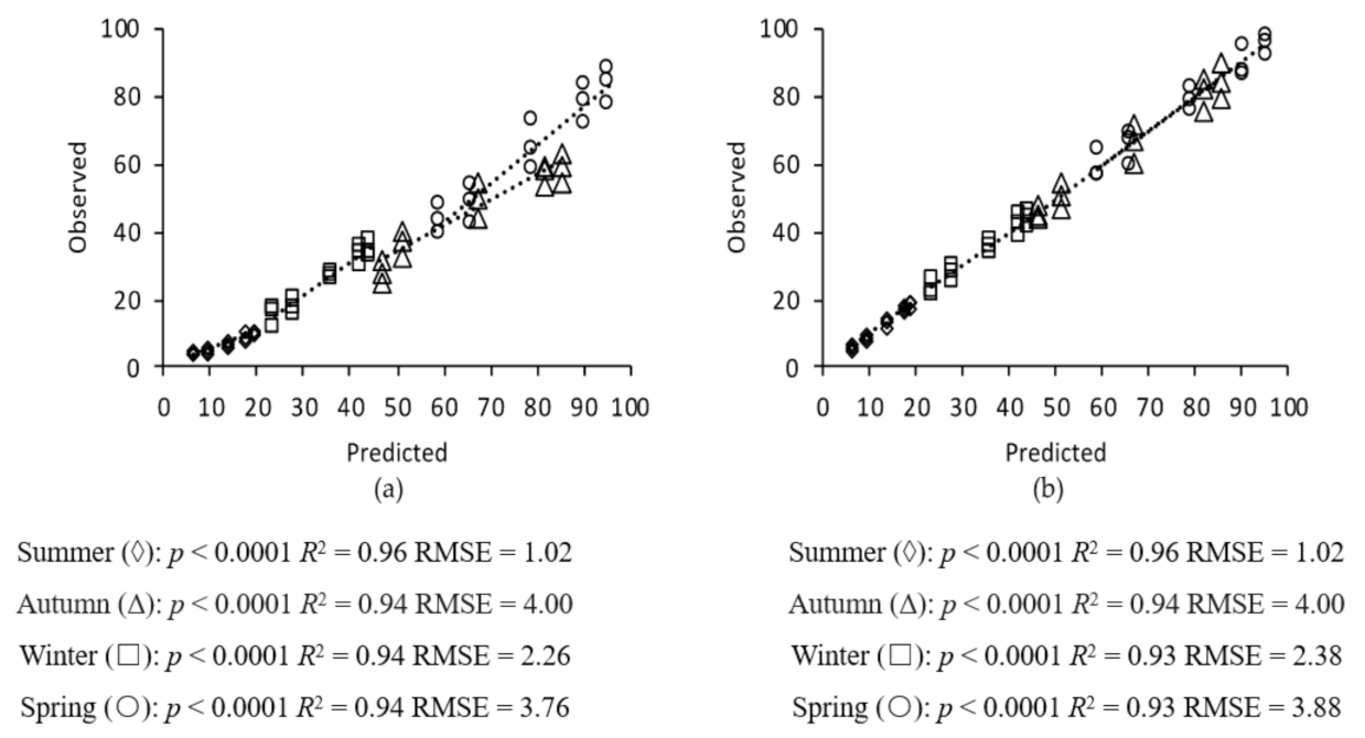
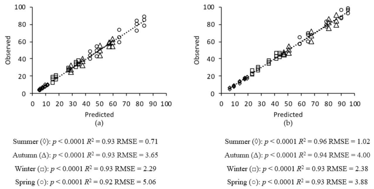
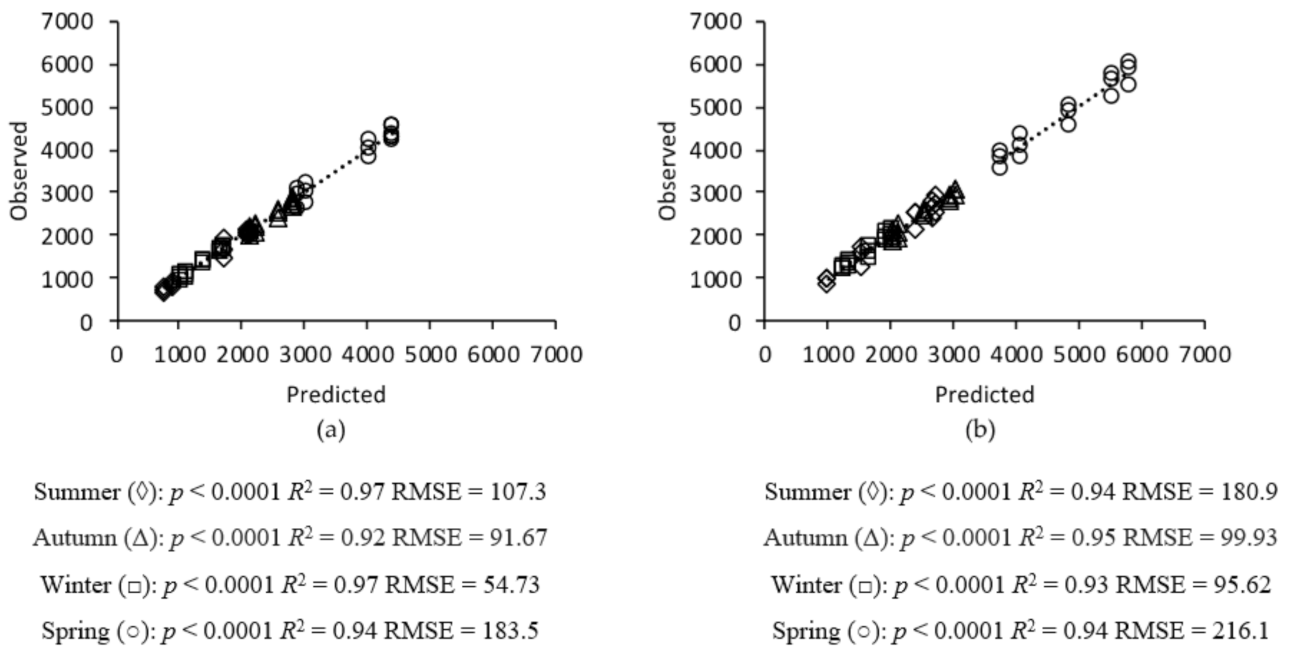
2.6. Model Validation

Models were validated according to accuracy, measured as the average distance between each observed data point and the equivalent predicted line.

$$Af = {10}^{\sum \left[\log \left(\frac{x_p}{x_b}\right)\right]∕n}$$

(9)

where x_p is the value of the specific maximum predictive growth rate (°C⁻¹), x_b is the value of the maximum specific observed growth rate (°C⁻¹), n is the number of observations, and Af is the accuracy value in the prediction.

The dataset used for validation of the models was obtained from samples collected in the same experimental plots (n = 300). This dataset was not used in the model development. Thus, models were cross-validated by evaluating the percent variation of data that could be explained by the model [25,26]. The percent variation was considered the coefficient of determination (R²) and was associated with the coefficient of correlation, which was developed using minimum squares [27].

3. Results

3.1. Grass Growth

A summary of the selection criteria for both models and species for both LBL and AHM is presented

Table 1. Selection criteria values to evaluate the Logistic and Gompertz models to predict the leaf blade length and accumulated herbage mass production as a function of the accumulated growing degree-days.

Species	Season	Model	Leaf Blade Length (cm)				Accumulated Herbage Mass (kg DM ha−1)
			AIC	BIC	RMSE	R2	AIC	BIC	RMSE	R2
L. perenne	Summer	Logistic	0.55	43.19	0.76	0.93	0.54	194.23	116.65	0.97
		Gompertz	0.45	43.61	0.77	0.93	0.46	194.57	117.96	0.97
	Autumn	Logistic	0.51	92.75	3.96	0.92	0.56	189.51	99.65	0.92
		Gompertz	0.49	92.84	3.97	0.92	0.44	189.98	101.23	0.92
	Winter	Logistic	0.51	78.66	2.48	0.93	0.57	174.03	59.50	0.97
		Gompertz	0.49	78.76	2.48	0.93	0.43	174.57	60.57	0.97
	Spring	Logistic	0.48	102.78	5.53	0.92	0.52	210.33	199.50	0.94
		Gompertz	0.52	102.61	5.50	0.92	0.48	210.52	200.77	0.94
B. valdivianus	Summer	Logistic	0.53	54.56	1.11	0.96	0.49	209.90	196.68	0.94
		Gompertz	0.47	54.83	1.12	0.96	0.51	209.79	195.95	0.94
	Autumn	Logistic	0.57	95.51	4.34	0.95	0.42	192.09	108.63	0.95
		Gompertz	0.43	96.06	4.42	0.94	0.58	191.46	106.36	0.95
	Winter	Logistic	0.54	78.46	2.46	0.94	0.61	190.77	103.95	0.93
		Gompertz	0.46	78.76	2.48	0.93	0.39	191.67	107.09	0.92
	Spring	Logistic	0.48	93.66	4.08	0.94	0.53	215.24	234.95	0.94
		Gompertz	0.52	93.51	4.06	0.94	0.47	215.48	236.88	0.94

L. perenne: Lolium perenne L., B. valdivianus: Bromus valdivianus Phil., AIC: Akaike information criterion, BIC: Bayesian information criterion, RMSE: Root-mean-square error, and R²: Determination coefficient.

. The Gompertz model presented the highest AIC values in the spring for both species (L. perenne and B. valdivianus) with 0.52 for LBL, whereas the Logistic model showed the lowest AIC value in the spring for both species with 0.48. The Gompertz model only had a lower BIC value in the spring when compared to the Logistic model. The R² and RMSE were similar between seasons and species (Figure 1, Figure 2, Figure 3 and Figure 4).

Table 2. Model parameterization of the four-parameter Logistic and Gompertz models for Lolium perenne L. and Bromus valdivianus Phil. during the four seasons of the year.

Species	Season	Model	Leaf Blade Length (cm)				Accumulated Herbage Mass (kg DM ha−1)
			a-GR	b-Pmax	c-AInf	d-ASup	a-GR	b-Pmax	c-AInf	d-ASup
L. perenne	Summer	Logistic	0.006 ± 0.003	303.9 ± 28.1	4.25 ± 0.74	11.45 ± 1.25	0.015 ± 0.004	244.9 ± 9.7	764.7 ± 74.3	2106 ± 52.2
		Gompertz	0.008 ± 0.004	288.1 ± 42.7	4.46 ± 0.55	12.67 ± 0.55	0.021 ± 0.004	222.3 ± 10.3	773.3 ± 67.8	2131 ± 62.7
	Autumn	Logistic	0.007 ± 0.003	220.1 ± 26.2	25.56 ± 5.79	60.12 ± 2.81	0.01 ± 0.005	249.1 ± 17.1	2116.9 ± 70.9	2822 ± 51.9
		Gompertz	0.01 ± 0.005	201.8 ± 19.8	28.3 ± 3.00	60.83 ± 3.33	0.02 ± 0.005	225.1 ± 18.2	2126 ± 58.3	2842 ± 66.3
	Winter	Logistic	0.009 ± 0.003	250.3 ± 17.2	14.86 ± 2.00	34.79 ± 1.5	0.009 ± 0.002	265.4 ± 11.9	1002 ± 47.3	1735 ± 44.1
		Gompertz	0.01 ± 0.004	227.5 ± 17.4	15.4 ± 1.45	35.53 ± 1.91	0.01 ± 0.003	242.8 ± 13.0	1023 ± 35.4	1776 ± 61.3
	Spring	Logistic	0.008 ± 0.003	262.5 ± 21.2	41.97 ± 4.87	84.32 ± 4.35	0.01 ± 0.008	242.9 ± 16.0	2912 ± 120.5	4415 ± 84.4
		Gompertz	0.01 ± 0.004	240.6 ± 21.3	43.6 2 ± 3.26	86.44 ± 5.66	0.02 ± 0.008	220.3 ± 16.2	2916 ± 114.6	4429 ± 95.2
B. valdivianus	Summer	Logistic	0.006 ± 0.002	245.4 ± 21.1	4.84 ± 1.91	19.71 ± 1.30	0.01 ± 0.003	204.8 ± 15.4	884.03 ± 197	2736 ± 97.2
		Gompertz	0.009 ± 0.003	224.6 ± 18.7	6.00 ± 1.08	20.44 ± 1.72	0.02 ± 0.005	188.1 ± 11.3	991.4 ± 117	2751 ± 107.2
	Autumn	Logistic	0.009 ± 0.003	264.5 ± 15.2	45.38 ± 3.37	86.0 ± 3.10	0.009 ± 0.003	266.1 ± 13.7	2007 ± 79.7	3067 ± 75.3
		Gompertz	0.01 ± 0.004	241.5 ± 16.7	46.40 ± 2.58	88.27 ± 4.34	0.01 ± 0.004	245.5 ± 14.4	2039 ± 60.4	3118 ± 97
	Winter	Logistic	0.007 ± 0.003	244.67 ± 21.7	22.2 ± 2.9	44.85 ± 2.00	0.008 ± 0.003	267.0 ± 18.6	1221 ± 83	2056 ± 79.3
		Gompertz	0.01 ± 0.004	221.9 ± 20	23.4 ± 1.73	45.78 ± 2.61	0.01 ± 0.004	242.3 ± 21.6	1237 ± 65	2113 ± 120
	Spring	Logistic	0.006 ± 0.002	256.54 ± 22.4	56.6 ± 5.15	97 ± 4.20	0.007 ± 0.003	264.2 ± 19.5	3699 ± 226.8	5891 ± 210.7
		Gompertz	0.01 ± 0.003	235 ± 20.8	59.1 ± 2.86	99 ± 5.33	0.01 ± 0.004	241.4 ± 20.3	3788 ± 151	6025 ± 294.3

Average ± standard error of L. perenne: Lolium perenne L., B. valdivianus: Bromus valdivianus Phil., GR: Growth rate, P_max: Point of maximum growth, A_Inf: Inferior asymptote, A_Sup: Superior asymptote.

presents the parameterization of both models for LBL and AHM. The Gompertz model exhibited the greatest values (between 0.008 and 0.01) for the slope of the tangent line to the inflection point across all seasons for LBL. The lowest slope value for GR was found with the Logistic model during the summer for L. perenne and B. valdivianus. This indicates a low GR for grass during this season, compared to those of autumn and spring. The slope values reported refer to the linear period of the exponential growth curve. The AHM exhibited the same pattern as LBL did, but with different values, varying from 0.007 to 0.021 (Table 2). The highest values for LBL and AHM were observed in the Gompertz model during the spring (99 cm and 6.025 kg DM ha⁻¹, respectively). The lowest values were found in the winter for both species in the Logistic model. The parameterization produced coordinates of AGDD X between 201.8 in the autumn and 303.9 in the summer for LBL. For AHM, the derivative varied between 188.1 and 267 AGDD, which was the maximum growth point at which the slope began to change (Table 2).

3.2. Nutritive Value

All nutritional variables were fitted to either a simple linear regression or a quadratic regression model. These models were adjusted in the range of 90–450 AGDD.

Table 3. Regression models for accumulated growing degree-days (X factor) versus nutritive value (Y factor) of Lolium perenne L. and Bromus valdivianus Phil. The standard error of each coefficient is presented in parentheses.

Variable	Species	Season	Model	R2	RMSE	p < |t|
CP (g 100 g−1)	L. Perenne	Summer	Y = 18.55(1.34) + 0.032(0.01) × AGDD−9.532e − 5(2.06 × 10−5) × AGDD2	0.87	1.08	0.001
		Autumn	Y = 27.98(0.36) − 0.02(0.001) × AGDD	0.96	0.60	0.001
		Winter	Y = 20.69(0.32) − 0.01(0.001) × AGDD	0.95	0.53	0.001
		Spring	Y = 22.92(0.54) − 0.03(0.001) × AGDD	0.96	0.90	0.001
	B. valdivianus	Summer	Y = 17.83(1.12) + 0.02(0.009) × AGDD − 7.6161 × 10−5 (1.73 × 10−5) × AGDD2	0.85	0.91	0.001
		Autumn	Y = 30.471(0.48) − 0.01(0.001) × AGDD	0.91	0.81	0.001
		Winter	Y = 23.88(0.32) − 0.02(0.001) × AGDD	0.96	0.54	0.001
		Spring	Y = 23.29(0.60) − 0.03(0.002) × AGDD	0.95	1.00	0.001
ME (Mcal kg DM−1)	L. perenne	Summer	Y = 2.24(0.06) + 0.002(5.1 × 10−4) × AGDD − 6.05 × 10−6 (9.2 × 10−7) × AGDD2	0.81	0.05	0.001
		Autumn	Y = 2.68(0.01) + 0.0003(8.6 × 10−5) × AGDD − 9.70 × 10−7 (1.5 × 10−7) × AGDD2	0.91	0.01	0.001
		Winter	Y = 2.61(3.03) + 2.6 × 10−4(3.6 × 10−4) × AGDD − 1.46 × 10−6 (5.5 × 10−7) × AGDD2	0.86	0.03	0.021
		Spring	Y = 2.59(0.02) + 2.6 × 10−4(2.2 × 10−4) × AGDD − 9.40 × 10−7 (4.0 × 10−7) × AGDD2	0.75	0.02	0.001
	B. valdivianus	Summer	Y = 2.29(0.02) + 7.2 × 10−4(1.7 × 10−4)×AGDD − 1.96 × 10−6 (3.1 × 10−7) × AGDD2	0.91	0.02	0.001
		Autumn	Y = 2.57(0.01) + 3.0 × 10−4(1.13 × 10−4)×AGDD − 7.64 × 10−7(2.1 × 10−7) × AGDD2	0.69	0.01	0.004
		Winter	Y = 2.50(0.02) + 7.3 × 10−5(2.2 × 10−4) × AGDD − 9.11 × 10−7(4.1 × 10−4) × AGDD2	0.87	0.02	0.049
		Spring	Y = 2.50(0.03) + 8.2 ×10−4 (2.5 × 10−4) × AGDD − 2.11 × 10−6 (4.6 × 10−7) × AGDD2	0.83	0.02	0.001
NDF (g 100 g−1)	L. perenne	Summer	Y = 42.37(0.45) + 0.01(0.001) × AGDD	0.78	0.75	0.001
		Autumn	Y = 39.56(0.60) + 0.03(0.002) × AGDD	0.95	1.00	0.001
		Winter	Y = 43.02(0.28) + 0.01(9.6 ×1 0−4) × AGDD	0.94	0.47	0.001
		Spring	Y = 35.08(1.29) + 0.06(0.004) × AGDD	0.93	2.13	0.001
	B. valdivianus	Summer	Y = 50.85(0.42) + 0.01(0.001) × AGDD	0.90	0.71	0.001
		Autumn	Y = 49.36(0.49) + 0.02(0.001) × AGDD	0.92	0.82	0.001
		Winter	Y = 50.10(0.37) + 0.01(0.001) × AGDD	0.91	0.61	0.001
		Spring	Y = 51.78(0.34) + 0.02(0.001) × AGDD	0.98	0.57	0.001
ADF (g 100 g−1)	L. Perenne	Summer	Y = 19.62(0.55) + 0.02(0.001) × AGDD	0.92	0.92	0.001
		Autumn	Y = 20.34(0.49) + 0.02(0.001) × AGDD	0.93	0.85	0.001
		Winter	Y = 20.90(0.70) + 0.01(0.002) × AGDD	0.93	0.59	0.001
		Spring	Y = 17.80(0.80) + 0.04(0.002) × AGDD	0.94	1.34	0.001
	B. valdivianus	Summer	Y = 28.23(0.47) + 0.01(0.001) × AGDD	0.87	0.78	0.001
		Autumn	Y = 23.70(0.49) + 0.02(0.001) × AGDD	0.92	0.81	0.001
		Winter	Y = 22.81(0.70) + 0.02(0.002) × AGDD	0.89	1.16	0.001
		Spring	Y = 20.51(0.80) + 0.03(0.002) × AGDD	0.94	1.33	0.001
WSC (g 1000 g−1)	L. Perenne	Summer	Y = 72.85(3.41) + 0.17(0.02) × AGDD − 1.8 × 10−4 (5.2 × 10−5) × AGDD2	0.93	2.75	0.004
		Autumn	Y = 89.71(4.88) + 0.17(0.04) × AGDD − 1.8 × 10−4 (7.5 × 10−5) × AGDD2	0.87	3.94	0.030
		Winter	Y = 74.46(5.27) + 0.20(0.01) × AGDD	0.90	8.71	0.001
		Spring	Y = 60.97(8.4) + 0.41(0.07) × AGDD − 4.7 × 10−4 (1.3e−04) × AGDD2	0.91	6.80	0.003
	B. valdivianus	Summer	Y = 67.71(3.43) + 0.16(0.02) × AGDD − 1.9 × 10−4 (5.2 × 10−5) × AGDD2	0.90	2.77	0.003
		Autumn	Y = 71.40(3.16) + 0.15(0.03) × AGDD − 1.6 × 10−4 (5.56 × 10−5) × AGDD2	0.91	2.92	0.013
		Winter	Y = 76.43(2.91) + 0.09(0.009) × AGDD	0.88	4.82	0.001
		Spring	Y = 80.56(3.87) + 0.14(0.03) × AGDD − 1.5 × 10−4 (5.9 × 10−5) × AGDD2	0.88	3.13	0.021

CP: Crude protein, ME: Metabolizable energy, NDF: Neutral detergent fiber, ADF: Acid detergent fiber, WSC: Water soluble carbohydrates, L. perenne: Lolium perenne L., B. valdivianus: Bromus valdivianus Phil., R²: Determination coefficient, RMSE: Root-mean-square error, AGDD: Accumulated growing degree-days, Y: Random variable to evaluate.

summarizes the models that best fitted the data for L. perenne and B. valdivianus across all seasons. The CP concentrations during the autumn, winter, and spring were best fitted by a linear regression, while the quadratic model was most accurate for summer data (R² = 0.87), autumn and spring (R² = 0.96). However, the response was similar between species.

The energy concentration decreased appreciably with plant maturity, affecting its nutritive value and consequently animal response. This quadratic pattern for the ME concentration can be explained graphically using a Gaussian function. The simple linear regression demonstrated the best fit to predict concentrations of ADF and NDF in both species in all seasons. The R² values varied from 0.78 for L. perenne in the summer to 0.98 for B. valdivianus in the summer and spring. The highest values of the b coefficient in the regression were obtained for B. valdivianus, demonstrating that this species has relatively higher ADF and NDF contents than L. perenne. The rate of change did not vary greatly between species, and all values were nonzero. The ADF and NDF concentrations increased proportionally with AGDD in both forage species, with 20% greater concentrations in B. valdivianus.

Both NDF and CP contents were greater in B. valdivianus than in L. perenne (Table 3). The AGDD was inversely proportional to the protein concentration, demonstrating that the CP content decreased as the pasture advanced in its growth cycle toward maturity. Thus, for every increase of 10 AGDD, the protein concentration decreased by 0.3 percent.

Both the ME and WSC had better predictions from the quadratic equations (higher R²). However, this was not true for WSC in the winter, where the linear regression showed a better fit for both species (Table 3). Early growth stages for these species, in which energy is stored, occur during the first 90 to 270 AGDD.

4. Discussion

4.1. Grass Growth

A variety of models can be used to describe and estimate grass growth and nutritive value under different environmental conditions. Complex models use exogenous and inherent grass variables as inputs to obtain precise calculations of the parameters [28,29], but many times, it is difficult for producers to collect all the necessary data. Therefore, a permanent challenge is the use of the minimum number of variables that provide a good estimation of grass growth and the model’s ease of use. In this study, TT and season were the only prediction variables used to determine the herbage mass and nutritive value of L. perenne and B. valdivianus, demonstrating that AGDD is a reliable tool [17]. The R² value greater than 0.9 and the low RMSE (Table 1) demonstrate that the Logistic and Gompertz models with TT as the prediction variable are accurate tools in the description and prediction of the LBL and AHM of L. perenne and B. valdivianus grass.

The differences found between seasons for the growth parameters can be primarily explained by the differences in metabolic activity in the grass over the course of the year. In the winter, the metabolic activity of plants can be reduced to 0 [30], and during the summer, the GR is reduced when optimal temperatures are exceeded [31]. During the spring and autumn, when there is an adequate balance between temperature and precipitation, grass metabolic activity can reach 90%, resulting in a greater GR [32]. Therefore, climate is an important factor regulating herbage production and nutritive value [33]. The sigmoid growth reported in this study, explained by both four-parameter models (Logistic and Gompertz) across seasons of the year, accurately described the grass growth, and they have been commonly used in studies that evaluate the growth dynamics of plant communities in different environments [34]. The development of these growth models and their parameters are important when comparing the GR of different species during the year to determine the most adequate DF. Other researchers that have used TT and HT as prediction variables in models to estimate grass growth have arrived at a similar conclusion; the sigmoid curve best describes the growth of a plant community, as it considers distinct developmental phases and is sufficiently robust [13].

The sinusoidal models to predict AHM present some limitations for L. perenne in the autumn and for B. valdivianus in the winter, resulting in less precise predictions in those seasons. In fact, a P_max growth of 40 AGDD was reached earlier than in the other seasons (Table 2). However, the maximum grass growth was estimated at 30 AGDD before what was observed in the field. Pulina et al. [35] suggested that these differences could be attributed to the sensitivity of the models to extreme values during data collection.

The parameters obtained and presented in this study agreed with those obtained by other researchers at different locations using other mathematical tools that integrate distinct climatic and soil variables [28,36]. Likewise, the effect of the AGDD on grass growth is clear and has been widely documented, suggesting that the effect of the AGDD on AHM is a nonlinear response [37].

4.2. Nutritive Value

Environmental conditions not only affect LBL and AHM, but also leaf appearance rate and grass phenology [38,39]. Therefore, it plays an important role in the establishment of grazing frequency, as nutrient concentration varies as a function of TT, season, and other factors [40,41]. The relationships found in the present study between AGDD and nutritive value across the different seasons of the year show a dependency in terms of quality in each species (Table 3). Robbins [42] reported an inverse linear reduction in the CP concentration and a direct linear relationship between the levels of NDF and ADF in grasses that had more AGDD at the defoliation time, which agreed with the current study.

The WSC patterns were similar in L. perenne and B. valdivianus and were best described by a quadratic model for summer, autumn, and spring. However, a linear model was best for winter, similarly to what was reported by Archontoulis and Miguez [10], as well as Bilge et al. [43]. This implies that in the winter, the herbage accumulated a greater WSC concentration explained by the continuation of photosynthesis and decreased growth, due to the lower temperatures. During the other seasons, grass growth continued at a higher rate than in winter, resulting in the use of the stored WSC [44,45]. Based on the quadratic model, WSC storage begins at 40 AGDD post-defoliation until approximately 270 to 360 AGDD. After that, the grass no longer accumulates WSC linearly, because of the favorable environmental conditions that allow grass growth and tissue renewal, which requires energy consumption. This is also shown by the fact that L. perenne and B. valdivanus have the highest concentrations of WSC during the winter.

The differences in values for the intercepts in the linear and quadratic regressions for seasons and species were relatively similar for most of the nutritive variables assessed. However, there were differences between seasons for NDF and ADF, with B. valdivianus having a greater intercept than L. perenne, and with autumn as the season that presented the lowest fiber concentration. Some studies have reported that this occurs because, in the spring, grass growth increases and quickly entering into the reproductive stage. This changes the leaf–stem ratio, and the maturation process requires the quick transport of nutrients to the roots and for seed formation [46,47].

Most models developed to evaluate grass quality have based their results on the NDF and ADF concentration, organic matter digestibility (OMD), CP, nitrogen indigestible in neutral detergent (NIND), and nitrogen indigestible in acid detergent (NIAD) [48,49,50]. However, few studies have incorporated ME. Some models have estimated their parameters based on the equations for net energy for lactation or maintenance (NE_L or NE_M, respectively) [51,52], and have considered the existing relationship between plant maturity and fiber, as well as CP and OMD. This is because during the plant growth cycle, the ME and CP decrease while the fiber concentration increases [53]. However, in this study, ME concentration was best described by a quadratic equation, because the observed data increased from the start until the asymptote was reached, at which point the slope was equal to 0. After this point, the values fell even lower than those initially observed due to increased plant maturity (Table 3). Other studies have used equations with this kind of pattern to describe similar biological processes in grasses, which supports the results herein presented [54,55].

Finally, the CP and fiber concentrations presented a negative linear relationship with AGDD for all seasons. This demonstrates that at greater AGDD, the protein levels of grasses decrease [56,57]. In general, the CP concentration was well represented by the linear regressions, which reported a variation in the RMSE of 1.08 for L. perenne in the summer and up to 0.53 and 0.54 for L. perenne and B. valdivianus, respectively, in the winter. These values were similar to those reported by other authors [58,59], who developed models using their own logarithms and adjusted these to a nitrogen consumption curve and integrated environmental variables such as precipitation and soil fertility. Regardless of the model used to explain the variations in CP concentration, all arrived at the same conclusion; the protein concentration decreased as the plant’s phenological age increased [60].

5. Conclusions

The grass growth of L. perenne and B. valdivianus over the course of the year in southern Chile can be accurately predicted by using both the four-parameter Logistic and Gompertz models by using AGDD as a predictor variable. Likewise, its nutritive value can be precisely predicted by using linear and quadratic regressions depending of the season of the year evaluated. The sinusoidal models were best suited to predict LBL and AHM, in every season and for both species.

References

1. McMaster, G.S.; Wilhelm, W. Growing degree-days: One equation, two interpretations. Agric. For. Meteorol. 1997, 87, 291–300. [Google Scholar] [CrossRef] [Green Version]
2. Elnesr, M.; Alazba, A. An integral model to calculate the growing degree-days and heat units, a spreadsheet application. Comput. Electron. Agric. 2016, 124, 37–45. [Google Scholar] [CrossRef]
3. Herz, K.; Dietz, S.; Haider, S.; Jandt, U.; Scheel, D.; Bruelheide, H. Predicting individual plant performance in grasslands. Ecol. Evol. 2017, 7, 8958–8965. [Google Scholar] [CrossRef]
4. Babu, R.; Rao, K.L.N.; Ashokarani, Y.; Martiluther, M.; Prasad, P.R.K. Prediction of phenological stages of six maize (Zea mays L.) hybrids based on required growing degree days. Int. J. Chem. Stud. 2020, 8, 2564–2574. [Google Scholar]
5. Ahanger, M.A.; Morad-Talab, N.; Abd-Allah, E.F.; Ahmad, P.; Hajiboland, R. Plant growth under drought stress: Significance of mineral nutrients. Water Stress Crop. Plants A Sustain. Approach 2016, 2, 649–668. [Google Scholar]
6. McMaster, G.S.; Wilhelm, W.W. Phenological responses of wheat and barley to water and temperature: Improving simulation models. J. Agric. Sci. 2003, 141, 129–147. [Google Scholar] [CrossRef] [Green Version]
7. Ostadian Bidgoly, R.; Balouchi, H.; Soltani, E.; Moradi, A. Effect of temperature and water potential on Carthamus tinctorius L. seed germination: Quantification of the cardinal temperatures and modeling using hydrothermal time. Ind. Crops. Prod. 2018, 113, 121–127. [Google Scholar] [CrossRef]
8. Kiniry, J.R.; Kim, S.; Williams, A.S.; Lock, T.R.; Kallenbach, R.L. Simulating bimodal tall fescue growth with a degree-day-based process-oriented plant model. Grass Forage Sci. 2018, 73, 432–439. [Google Scholar] [CrossRef]
9. Hunt, R.C.; Shipley, B.R.; Askew, A.P. A Modern Tool for Classical Plant Growth Analysis. Ann. Bot. 2002, 90, 485–488. [Google Scholar] [CrossRef] [PubMed] [Green Version]
10. Archontoulis, S.V.; Miguez, F.E. Nonlinear Regression Models and Applications in Agricultural Research. Agron. J. 2015, 107. [Google Scholar] [CrossRef] [Green Version]
11. Paine, C.E.T.; Marthews, T.R.; Vogt, D.R.; Purves, D.; Rees, M.; Hector, A.; Turnbull, L.A. How to fit nonlinear plant growth models and calculate growth rates: An update for ecologists. Methods Ecol. Evol. 2012, 3, 245–256. [Google Scholar] [CrossRef]
12. Hoffmann, W.A.; Poorter, H. Avoiding Bias in Calculations of Relative Growth Rate. Ann. Bot. 2002, 90, 37–42. [Google Scholar] [CrossRef] [Green Version]
13. Thornley, J.H.; France, J. Mathematical Models in Agriculture: Quantitative Methods for the Plant, Animal and Ecological Sciences, 2nd ed.; CABI: Wallingford, UK, 2007; pp. 136–208. [Google Scholar]
14. Zhao, J.; Zhao, Y.; Song, Z.; Liu, H.; Liu, Y.; Yang, R. Genetic analysis of the main growth traits using random regression models in Japanese flounder (Paralichthys olivaceus). Aquac. Res. 2018, 49, 1504–1511. [Google Scholar] [CrossRef]
15. Choler, P. Growth response of temperate mountain grasslands to inter-annual variations in snow cover duration. Biogeosciences 2015, 12, 3885–3897. [Google Scholar] [CrossRef] [Green Version]
16. McClung, C.R.; Davis, S.J. Ambient thermometers in plants: From physiological outputs towards mechanisms of thermal sensing. Curr. Biol. 2010, 20, R1086–R1092. [Google Scholar] [CrossRef] [Green Version]
17. Calvache, I.; Balocchi, O.; Alonso, M.; Keim, J.P.; López, I.F. Thermal Time as a Parameter to Determine Optimal Defoliation Frequency of Perennial Ryegrass (Lolium perenne L.) and Pasture Brome (Bromus valdivianus Phil.). Agronomy 2020, 10, 620. [Google Scholar] [CrossRef]
18. Monteith, J.L. Climate and the efficiency of crop production in Britain. Philos. Trans. R. Soc. Lond. B Biol. Sci. 1977, 281, 277–294. [Google Scholar]
19. Thompson, R.; Clark, R.M. Spatio-temporal modelling and assessment of within-species phenological variability using thermal time methods. Int. J. Biometeorol. 2006, 50, 312–322. [Google Scholar] [CrossRef]
20. Biligetu, B.; Coulman, B. Responses of Three Bromegrass (Bromus) Species to Defoliation under Different Growth Conditions. Int. J. Agron. 2010, 2010, 1–5. [Google Scholar] [CrossRef] [Green Version]
21. Pan, J.; Zhu, Y.; Cao, W.; Dai, T.; Jiang, D. Predicting the protein content of grain in winter wheat with meteorological and genotypic factors. Plant. Prod. Sci. 2006, 9, 323–333. [Google Scholar] [CrossRef]
22. Leys, C.; Ley, C.; Klein, O.; Bernard, P.; Licata, L. Detecting outliers: Do not use standard deviation around the mean, use absolute deviation around the median. J. Exp. Soc. Psychol. 2013, 49, 764–766. [Google Scholar] [CrossRef] [Green Version]
23. Mohammed, E.A.; Naugler, C.; Far, B.H. Emerging Business Intelligence Framework for a Clinical Laboratory through Big Data Analytics. Emerging Trends in Computational Biology, Bioinformatics, and Systems Biology: Algorithms and Software Tools; Elsevier/Morgan Kaufmann: New York, NY, USA, 2015; Chapter 32; pp. 577–602. [Google Scholar]
24. Coleman, S.W.; Henry, D.A. Nutritive value of herbage. In Sheep Nutrition; Freer, M., Dove, H., Eds.; CSIRO Publishing: Collingwood, UK, 2002; pp. 1–26. [Google Scholar]
25. Chuine, I.; Cour, P.; Rousseau, D. Selecting models to predict the timing of flowering of temperate trees: Implications for tree phenology modelling. Plant Cell Environ. 1999, 22, 1–13. [Google Scholar] [CrossRef] [Green Version]
26. Fan, X.; Kawamura, K.; Guo, W.; Xuan, T.D.; Lim, J.; Yuba, N.; Kurokawa, Y.; Obitsu, T.; Lv, R.; Tsumiyama, Y.; et al. A simple visible and near-infrared (V-NIR) camera system for monitoring the leaf area index and growth stage of Italian ryegrass. Comput. Electron. Agric. 2018, 144, 314–323. [Google Scholar] [CrossRef]
27. Karimi, S.; Sadraddini, A.A.; Nazemi, A.H.; Xu, T.; Fard, A.F. Generalizability of gene expression programming and random forest methodologies in estimating cropland and grassland leaf area index. Comput. Electron. Agric. 2018, 144, 232–240. [Google Scholar] [CrossRef]
28. Li, Q.; Xu, L.; Pan, X.; Zhang, L.; Li, C.; Yang, N.; Qi, J. Modeling phenological responses of Inner Mongolia grassland species to regional climate change. Environ. Res. Lett. 2016, 11, 015002. [Google Scholar] [CrossRef]
29. Yan, W.; Wallace, D.H.; Ross, J. A Model of Photoperiod × Temperature Interaction Effects on Plant Development. Crit. Rev. Plant. Sci. 2011, 15, 63–96. [Google Scholar]
30. Orloff, S.B.; Brummer, E.C.; Shrestha, A.; Putnam, D.H. Cool-Season Perennial Grasses Differ in Tolerance to Partial-Season Irrigation Deficits. Agron. J. 2016, 108, 692–700. [Google Scholar] [CrossRef]
31. Bartholomew, P.W. Effect of Varying Temperature Regime on Phyllochron in Four Warm-Season Pasture Grasses. Agric. Sci. 2014, 5, 1000–1006. [Google Scholar] [CrossRef]
32. Ruelland, E.; Zachowski, A. How plants sense temperature. Environ. Exp. Bot. 2010, 69, 225–232. [Google Scholar] [CrossRef]
33. Rapacz, M.; Ergon, A.; Hoglind, M.; Jorgensen, M.; Jurczyk, B.; Ostrem, L.; Rognli, O.A.; Tronsmo, A.M. Overwintering of herbaceous plants in a changing climate. Still more questions than answers. Plant. Sci. 2014, 225, 34–44. [Google Scholar] [CrossRef]
34. Lanier, W.E.; Bailey, L.L.; Muths, E. Integrating biology, field logistics, and simulations to optimize parameter estimation for imperiled species. Ecol. Model. 2016, 335, 16–23. [Google Scholar] [CrossRef]
35. Pulina, A.; Lai, R.; Salis, L.; Seddaiu, G.; Roggero, P.P.; Bellocchi, G. Modelling pasture production and soil temperature, water and carbon fluxes in Mediterranean grassland systems with the Pasture Simulation model. Grass Forage Sci. 2018, 73, 272–283. [Google Scholar] [CrossRef] [Green Version]
36. Ikeda, H.; Okamoto, K.; Fukuhara, M. Estimation of aboveground grassland phytomass with a growth model using Landsat TM and climate data. Int. J. Remote Sens. 2010, 20, 2283–2294. [Google Scholar] [CrossRef]
37. Chen, N.; Zhang, Y.; Zhu, J.; Li, J.; Liu, Y.; Zu, J.; Wang, L. Nonlinear responses of productivity and diversity of alpine meadow communities to degradation. Chin. J. Plant. Ecol. 2018, 42, 50–65. [Google Scholar]
38. Bai, Y.; Wu, J.; Clark, C.M.; Pan, Q.; Zhang, L.; Chen, S.; Wang, Q.; Han, X.; Wisley, B. Grazing alters ecosystem functioning and C:N:P stoichiometry of grasslands along a regional precipitation gradient. J. Appl. Ecol. 2012, 49, 1204–1215. [Google Scholar] [CrossRef]
39. Belesky, D.; Ruckle, J.; Abaye, A. Seasonal distribution of herbage mass and nutritive value of Prairiegrass (Bromus catharticus Vahl). Grass Forage Sci. 2007, 62, 301–311. [Google Scholar] [CrossRef]
40. Davidson, A.; Da Silva, D.; Quintana, B.; DeJong, T.M. The phyllochron of Prunus persica shoots is relatively constant under controlled growth conditions but seasonally increases in the field in ways unrelated to patterns of temperature or radiation. Sci. Hortic. 2015, 184, 106–113. [Google Scholar] [CrossRef]
41. Kumudini, S.; Andrade, F.H.; Boote, K.J.; Brown, G.A.; Dzotsi, K.A.; Edmeades, G.O.; Gocken, T.; Goodwin, M.; Halter, A.L.; Hammer, G.L.; et al. Predicting Maize Phenology: Intercomparison of Functions for Developmental Response to Temperature. Agron. J. 2014, 106, 2087–2097. [Google Scholar] [CrossRef] [Green Version]
42. Robins, J.G. Evaluation of warm-season grasses nutritive value as alternatives to cool-season grasses under limited irrigation. Grassl. Sci. 2016, 62, 144–150. [Google Scholar] [CrossRef]
43. Bilge, A.H.; Ozdemir, Y. Determining the Critical Point of a Sigmoidal Curve via its Fourier Transform. J. Phys. Conf. Ser. 2016, 738, 012062. [Google Scholar] [CrossRef] [Green Version]
44. Pontes, L.S.; Carrere, P.; Andueza, D.; Louault, F.; Soussana, J. Seasonal productivity and nutritive value of temperate grasses found in semi-natural pastures in Europe: Responses to cutting frequency and N supply. Grass Forage Sci. 2007, 62, 485–496. [Google Scholar] [CrossRef]
45. Ren, H.; Han, G.; Lan, Z.; Wan, H.; Schönbach, P.; Gierus, M.; Taube, F. Grazing effects on herbage nutritive values depend on precipitation and growing season in Inner Mongolian grassland. J. Plant. Ecol. 2016, 9, 712–723. [Google Scholar] [CrossRef] [Green Version]
46. Mládek, J.; Hejcman, M.; Hejduk, S.; Duchoslav, M.; Pavlů, V. Community Seasonal Development Enables Late Defoliation Without Loss of Forage Quality in Semi-natural Grasslands. Folia Geobot. 2010, 46, 17–34. [Google Scholar] [CrossRef]
47. Sanderson, M.A.; Stout, R.; Brink, G. Productivity, Botanical Composition, and Nutritive Value of Commercial Pasture Mixtures. Agron. J. 2016, 108, 450–456. [Google Scholar] [CrossRef]
48. Bertilsson, J.; Akerlind, M.; Eriksson, T. The effects of high-sugar ryegrass/red clover silage diets on intake, production, digestibility, and N utilization in dairy cows, as measured in vivo and predicted by the NorFor model. J. Dairy Sci. 2017, 100, 7990–8003. [Google Scholar] [CrossRef] [PubMed]
49. Gauch, H.G.; Hwang, J.T.; Fick, G.W. Model evaluation by comparison of model-based predictions and measured values. Agron. J. 2003, 95, 1442–1446. [Google Scholar] [CrossRef] [Green Version]
50. Ruelle, E.; Hennessy, D.; Delaby, L. Development of the Moorepark St Gilles grass growth model (MoSt GG model): A predictive model for grass growth for pasture based systems. Eur. J. Agron. 2018, 99, 80–91. [Google Scholar] [CrossRef]
51. Bruinenberg, M.; Valk, H.; Korevaar, H.; Struik, P. Factors affecting digestibility of temperate forages from seminatural grasslands: A review. Grass Forage Sci. 2002, 57, 292–301. [Google Scholar] [CrossRef]
52. Lee, J.M.; Clark, A.J.; Roche, J.R. Climate-change effects and adaptation options for temperate pasture-based dairy farming systems: A review. Grass Forage Sci. 2013, 68, 485–503. [Google Scholar] [CrossRef]
53. Tasset, E.; Boulanger, T.; Diquélou, S.; Laîné, P.; Lemauviel-Lavenant, S. Plant trait to fodder quality relationships at both species and community levels in wet grasslands. Ecol. Indic. 2019, 97, 389–397. [Google Scholar] [CrossRef]
54. Cao, R.; Francisco-Fernández, M.; Anand, A.; Bastida, F.; González-Andújar, J.L. Modeling Bromus diandrus seedling emergence using nonparametric estimation. J. Agric. Biol. Environ. Stat. 2013, 18, 64–86. [Google Scholar] [CrossRef] [Green Version]
55. Insua, J.R.; Agnusdei, M.G.; Berone, G.D.; Basso, B.; Machado, C.F. Modeling the Nutritive Value of Defoliated Tall Fescue Pastures Based on Leaf Morphogenesis. Agron. J. 2019, 111, 714–724. [Google Scholar] [CrossRef]
56. Loaiza, P.A.; Balocchi, O.; Bertrand, A. Carbohydrate and crude protein fractions in perennial ryegrass as affected by defoliation frequency and nitrogen application rate. Grass Forage Sci. 2017, 72, 556–567. [Google Scholar] [CrossRef]
57. Smart, A.J.; Schacht, W.H.; Volesky, J.D.; Moser, L.E. Seasonal Changes in Dry Matter Partitioning, Yield, and Crude Protein of Intermediate Wheatgrass and Smooth Bromegrass. Agron. J. 2006, 98, 986–991. [Google Scholar] [CrossRef] [Green Version]
58. Jing, Q.; Jégo, G.; Bélanger, G.; Chantigny, M.H.; Rochette, P. Simulation of water and nitrogen balances in a perennial forage system using the STICS model. Field Crop. Res. 2017, 201, 10–18. [Google Scholar] [CrossRef]
59. Persson, T.; Höglind, M.; Van Oijen, M.; Korhonen, P.; Palosuo, T.; Jégo, G.; Virkajärvi, P.; Bélanger, G.; Gustavsson, A.M. Simulation of timothy nutritive value: A comparison of three process-based models. Field Crop. Res. 2019, 231, 81–92. [Google Scholar] [CrossRef]
60. Frary, A. Plant Physiology and Development. Rhodora 2015, 117, 397–399. [Google Scholar] [CrossRef]
Figure 1. Observed v. predicted data for leaf blade length as calculated by the four-parameter Logistic model for Lolium perenne L. (a) and Bromus valdivianus Phil (b). R2 = Determination coefficient.; RMSE = Root mean square error.
Agronomy 11 00774 g001
Figure 2. Observed v. predicted data for leaf blade length as calculated by the four-parameter Gompertz model for Lolium perenne L. (a) and Bromus valdivianus Phil (b). R2 = Determination coefficient.; RMSE = Root mean square error.
Agronomy 11 00774 g002
Figure 3. Observed v. predicted data for accumulated herbage mass production according to the four-parameter Logistic model for Lolium perenne L. (a) and Bromus valdivianus Phil (b). R2 = Determination coefficient.; RMSE = Root mean square error.
Agronomy 11 00774 g003
Figure 4. Observed v. predicted data for accumulated herbage mass production according to the four-parameter Gompertz model for Lolium perenne L. (a) and Bromus valdivianus Phil (b). R2 = Determination coefficient.; RMSE = Root mean square error.
Agronomy 11 00774 g004