Comparative Analysis of Statistical Regression Models for Prediction of Live Weight of Korean Cattle during Growth

Abstract

Measuring weight during cattle growth is essential for determining their status and adjusting the feed amount. Cattle must be weighed on a scale, which is laborious and stressful and could hinder growth. Therefore, automatically predicting cattle weight could reduce stress on cattle and farm laborers. This study proposes a prediction system to measure the change in weight automatically during growth using three regression models, using environmental factors, feed intake, and weight during the period. The Bayesian inference and likelihood estimation principles estimate parameters that determine the models: the weighted regression model (WRM), Gaussian process regression model (GPRM), and Gaussian process panel model (GPPM). A posterior distribution was derived using these parameters, and a weight prediction system was implemented. An experiment was conducted using image data to evaluate model performance. The GPRM with the squared exponential kernel had the best predictive power. Next, GPRMs with polynomial and rational quadratic kernels, the linear model, and WRM had the next-best predictive power. Finally, the GPRM with the linear kernel, the linear model, and the latent growth curve model, and types of GPPM had the next-best predictive power. GPRM and WRM are statistical probability models that apply predictions to the entire cattle population. These models are expected to be useful for predicting cattle growth on farms at a population level. However, GPPM is a statistical probability model designed for measuring the weight of individual cattle. This model is anticipated to be more efficient when predicting the weight of individual cattle on farms.

1. Introduction

Monitoring, recording, and predicting livestock body weight is essential for individual animal health management, timely dietary interventions, improved genetic selection efficiency, and identifying the optimal timing for livestock market placement. Animals that have already reached the point of slaughter become a liability to the livestock operation, as they no longer contribute to overall weight gain [1]. In addition, rapid changes in the body weight of livestock can be used to control feed intake, determine whether they are infected with diseases, and detect abnormal health conditions.

Information, such as age, sex, genotype, volume, and area, is needed, along with various physical characteristics of the livestock, to predict the weight of livestock accurately. In addition, to estimate the change in body weight accurately for each growth stage of the livestock, the body weight measurements must be repeated several times for each growth stage [2,3]. However, multiple manual measurements of animal body dimensions are labor-intensive, time-consuming, and expensive. Moreover, they are also stressful for the animals and workers [4].

Therefore, to address these issues, there has been a growing interest in adopting a noncontact weighing method that utilizes cost-effective sensors and machine vision technology as an alternative to the labor-intensive and stress-inducing process of direct animal weight measurement. In response to these practical demands, numerous studies aiming to automate the prediction of livestock weight have been carried out, divided into three main areas using classical regression models, growth curve models, machine learning, and deep learning techniques.

We briefly review these previously proposed methods. Research using linear regression models with image analysis and body measurements [5,6], studies employing neutral linear regression models [7], region-specific models for West Africa [8,9], and research identifying critical dimensions through image and measurement analysis have been conducted.

Second, various researchers have utilized growth curve models proposed in the literature to predict livestock growth weight. Some of them employed nonlinear growth models [10] to model and predict growth curves for livestock such as pigs, cattle, rabbits, and sheep [11,12]. Additionally, models considering causality [13] and models using Bayesian frameworks [14] have been developed and applied to real animal populations. Through comparisons of various models, logistic and Richards models [15] were identified as the most suitable models for specific animals. Furthermore, nonlinear growth curve models [16] have been used to assess performance and predict breeding management and growth rates in animals.

Third, various studies have explored methods for predicting livestock weight using machine learning, deep learning, and image processing techniques. These studies include predictions of live weight and carcass characteristics through 3D imaging and machine learning algorithms [17], shape feature extraction from 3D images for weight prediction using linear regression [18], a review of computer vision and machine learning-based weight prediction methods with a discussion of their strengths and weaknesses [1], comparisons between traditional linear regression models and different machine learning algorithms for weight prediction in cattle [19], a novel live weight prediction model based on 3D cloud augmentation and deep learning image regression [4], a comparative examination of machine learning techniques for predicting live cattle weight [20], automatic Korean cattle weight prediction using the Bayesian ridge algorithm and body characteristic extraction from RGB-D images [21], weight prediction performance comparisons on 3D cow image data using various supervised learning techniques [22], and cow weight estimation using semantic segmentation and stereo vision in computer vision [23].

Finally, Oliveira et al. [24] published a comprehensive review paper on the deep learning algorithms for computer vision systems that can be used in livestock breeding. Most studies have used classical linear regression models, growth curve models, and machine and deep learning analyses to predict livestock weight. However, the relationship between body weight, biological characteristics, and feed intake is complex and nonlinear; thus, it seems more appropriate to use a statistical probability model considering the growth age of livestock to predict livestock weight accurately.

This paper considers three statistical regression models, the weighted regression model (WRM), the Gaussian process regression model (GPRM), and the Gaussian process panel model (GPPM), to predict the actual weight during the growth process of Korean cattle based on feed intake and age. It is a comparison of curve models and various machine learning and deep learning methods.

This paper makes the following main contributions. Firstly, we propose three enhanced regression models, namely WRM, GPRM, and GPPM, aimed at more accurately predicting the weight of field-raised cattle. These models improve upon the commonly used linear regression model for cow weight prediction. Secondly, we introduce the principles of Bayesian inference and likelihood estimation as methods for estimating the parameters that define the hypothesized regression models. We also describe the process of deriving the posterior distribution for predicted values using these principles. Thirdly, we present the results of comparing and evaluating the predictive performance of the three proposed regression models using the widely utilized R package in the field of statistics.

The structure of the paper is outlined as follows. Section 2 introduces the collected data and outlines the derivation process of the posterior distribution, which is capable of predicting the weight of a cow based on these data. Section 3 describes the experimental procedure and presents the results used to assess the performance of the three proposed regression models. Section 4 provides a discussion of the results. Finally, Section 5 summarizes the conclusions of this paper and outlines potential directions for future research.

2. Materials and Methods

2.1. Data Collection

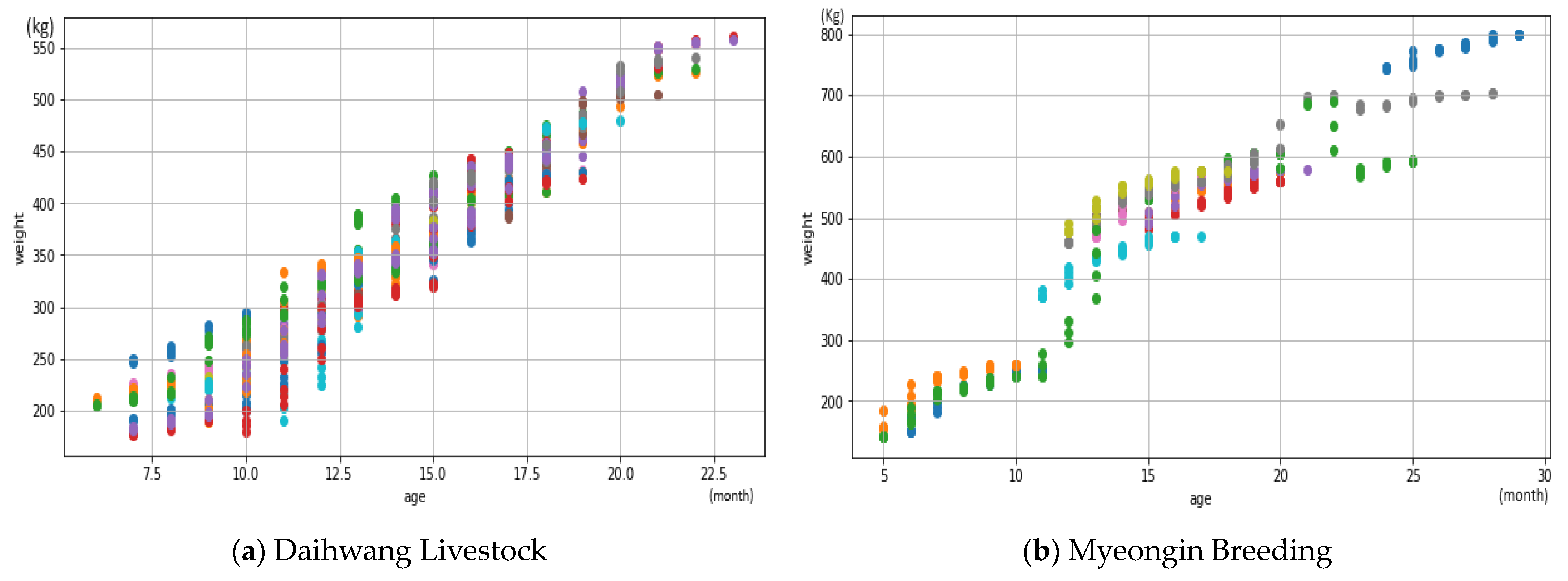
The necessary data for the analysis were collected from 15 and 13 Korean male cattle raised in two livestock farms (Daihwang Livestock and Myeongin Breeding, respectively) in South Jeolla-do (province), Korea. First, Daihwang Livestock farmers collected data by measuring the livestock 45 times weekly from 23 August 2021 to 30 June 2022. Furthermore, the master breeding farmhouse collected data by repeating 26 measurements weekly from 15 July 2021 to 30 December 2021. Second, measurements were taken for three biological characteristics of Korean cattle (body weight, age, and chest width) and four environmental factors (maximum temperature, average precipitation, average humidity, and cumulative sunlight). These data are summarized in

Table 1. Summary of data collected from Korean cattle farms.

Livestock Farm	No. of Cattle	No. of Repetitions	No. of Data	Measurements
Daihwang Livestock	15	45	675	Cattle weight, three biological characteristics, four environmental factors
Myeongin Breeding	13	26	338

.

2.2. Analysis Methods

We examined the mathematical aspects of three stochastic regression models designed for predicting the live weight of Korean cattle as they progress through their growth stages.

2.2.1. Weighted Regression Model

The WRM can be used when the ordinary regression model’s assumption that the variance of the errors is constant is violated (called heteroscedasticity). The WRM for data with k explanatory variables and n response measures can be represented in vector format as follows:

$$\mathit{y}=f\left(\mathit{X}\right)+\mathit{ϵ}=\mathit{X}\mathit{\beta }+\mathit{ϵ},$$

(1)

where $\mathit{y}$ denotes an $n\times 1$ response vector,$\mathit{X}$ indicates an $n\times k$ explanatory matrix, $\mathit{\beta }$ represents a $k\times 1$ parameter vector, and we assume that ϵ follows a (multivariate) normal distribution with a mean vector of zero, denoted as 0, and a non-constant variance—covariance matrix Σ.

Therefore, we obtain:

$$\mathit{y} ~ N\left(\mathit{X}\mathit{\beta }, \Sigma \right).$$

(2)

The weighted least squares estimate for parameter vector $\mathit{\beta }$ is obtained by minimizing the sum of square error:

$$\widehat{\mathit{\beta }}={\mathrm{argmin}}_{\mathit{\beta }} {\mathit{ϵ}}^T\mathit{ϵ},={\left(\mathit{X}\Sigma \mathit{X}\right)}^{-1}{\mathit{X}}^T\mathit{W}\mathit{y}.$$

(3)

Finally, when an explanatory value is represented as x, the forecasted value of the corresponding response variable is as follows:

$$\widehat{y}={\mathbf{x}}^T\widehat{\mathit{\beta }}.$$

(4)

2.2.2. Gaussian Process Regression Model

Gaussian process regression (GPR) model extends the linear regression model described in Equation (1) to accommodate nonlinear relationships between the response variable $\mathit{y}$ and the input vector $\mathbf{x}$ [25,26]. This is achieved by introducing a function $\mathsf{\phi }\left(\mathbf{x}\right)$ that transforms the input vector $\mathbf{x}$ into a new space [26]:

$$\mathrm{f}\left(\mathbf{x}\right)= \mathsf{\phi }{\left(\mathbf{x}\right)}^T\mathit{\beta }.$$

(5)

Next, GPR uses Bayesian inference; thus, we must assume a prior distribution for the coefficient vector $\mathit{\beta }$. We consider the subsequent multivariate normal distribution as the prior distribution for the coefficient vector$\mathit{\beta }$:

$$\mathit{\beta } ~ MVN\left({\mathit{\mu }}_{\mathit{\beta }}, {\Sigma }_{\mathit{\beta }}\right).$$

(6)

In addition, using the properties of a normal distribution and variable transformation, the prior distribution of the regression function $\mathrm{f}\left(\mathbf{X}\right)={\left[\left(f(x_1\right),\cdots ,f\left(x_n\right)\right]}^T$ for a matrix $\mathit{X}$ with an input vector as a column is given as the following multivariate normal distribution:

$$\mathrm{f}\left(\mathbf{X}\right)=\phi {\left(\mathit{X}\right)}^T\mathit{\beta } ~ MVN\left(\phi {\left(\mathit{X}\right)}^T{\mathit{\mu }}_{\mathit{\beta }}, \phi {\left(\mathit{X}\right)}^T{\Sigma }_{\mathit{\beta }}\phi \left(\mathit{X}\right)\right).$$

(7)

Hence, the prior distribution of the regression function for a finite input vector $\mathbf{x}$ is represented using a multivariate Gaussian distribution [26]. However, when the input vector $\mathbf{x}$ is infinite, representing it as a Gaussian distribution becomes impossible. In such cases, a probabilistic process is needed, and among them, the Gaussian stochastic process is the most suitable for the data.

The Gaussian stochastic process is characterized by the property that a subset of random vectors follows a multivariate Gaussian distribution. To fully describe the prior distribution of the regression function, we need to specify the distribution of the Gaussian process $\left\{f\left(\mathbf{x}\right), \mathbf{x}\in \mathcal{X}\right\}$. This Gaussian process is described by a mean function and a kernel [26]. This is abbreviated as:

$$Y\left(\mathbf{x}\right) ~ GP(\phi {\left(\mathbf{x}\right)}^T{\mathit{\mu }}_{\mathit{\beta }}, \phi {\left(\mathbf{x}\right)}^T{\Sigma }_{\mathit{\beta }}\phi \left(\mathbf{x}\right)+\mathit{W}).$$

(8)

Hence, the GPR model fully characterizes the outcome variable $Y\left(\mathbf{x}\right)$ using a mean function and a kernel. The specification of this model involves the selection of both the mean function and the kernel. In GPR, the primary focus of inference is primarily on achieving optimal predictions, which necessitates splitting the data into training and testing sets. The training set is utilized to train the model with the objective of obtaining optimal predictions for input vectors not present in the training set. GPR directly computes the predictive distribution in a single step [26]. The predictive distribution signifies the distribution provided the model and training set for predictions on the testing set, denoted as $f({\mathit{X}}^{\ast }|D)$. For the sake of clarity in notation, we introduce the following:

$$\mathit{M}\left(\mathbf{X}\right)=\left[\begin{array}{c}m\left(X_1\right)\\ m\left(X_2\right)\\ \begin{array}{c}⋮\\ m\left(X_{N_1}\right)\end{array}\end{array}\right], \mathit{K}\left(\mathit{X}, {\mathit{X}}^{\ast }\right)=\left[\begin{array}{ccc}k\left({\mathbf{x}}_1,{\mathbf{x}}_1^{\ast }\right)& \cdots & k\left({\mathbf{x}}_1,{\mathbf{x}}_{N_2}^{\ast }\right)\\ ⋮& \cdots & ⋮\\ k\left({\mathbf{x}}_{N_1},{\mathbf{x}}_1^{\ast }\right)& \cdots & k\left({\mathbf{x}}_{N_1},{\mathbf{x}}_{N_2}^{\ast }\right)\end{array}\right].$$

(9)

This approach enables us to represent the joint distribution of observations $Y\left(\mathit{X}\right)$ and predictions $f\left({\mathit{X}}^{\ast }\right)$ as follows [26]:

$$\left[\begin{array}{c}Y\left(\mathit{X}\right)\\ f\left({\mathit{X}}^{\ast }\right)\end{array}\right]=N(M\left(\begin{array}{c}\mathit{X}\\ {\mathit{X}}^{\ast }\end{array}\right), \left[\begin{array}{cc}K\left(\mathit{X},\mathit{X}\right)+W& K\left(\mathit{X},{\mathit{X}}^{\ast }\right)\\ K\left({\mathit{X}}^{\ast }, \mathit{X}\right)& K\left({\mathit{X}}^{\ast },{\mathit{X}}^{\ast }\right)\end{array}\right].$$

(10)

The predictive distribution is derived by conditioning on the observations $\mathit{y}\left(\mathit{X}\right)$, and it has an analytical solution [26]:

$$f({\mathit{X}}^{\ast }|D) ~ N\left(E(f\left({\mathit{X}}^{\ast }\right)|D\right), \mathrm{Cov}(f\left({\mathit{X}}^{\ast }\right)|D)) \mathrm{with}$$

(11)

$$E(f\left({\mathit{X}}^{\ast }\right)|D)=M\left({\mathit{X}}^{\ast }\right)+K\left({\mathit{X}}^{\ast }, \mathit{X}\right){\left[K\left(\mathit{X},\mathit{X}\right)+W \right]}^{-1}\left(\mathbf{y}-\mathit{M}\left(\mathbf{X}\right)\right),$$

(12)

$$\mathrm{Cov}\left(f\left({\mathit{X}}^{\ast }\right)|D\right)=K\left({\mathit{X}}^{\ast },{\mathit{X}}^{\ast }\right)-K\left({\mathit{X}}^{\ast }, \mathit{X}\right){\left[K\left(\mathit{X},\mathit{X}\right)+W\right]}^{-1}K\left(\mathit{X},{\mathit{X}}^{\ast }\right).$$

(13)

2.2.3. Gaussian Process Panel Model

We extend GPR to introduce the Gaussian process panel model (GPPM) for predicting Korean cattle weight [27,28]. In a longitudinal dataset, we observe $N\in \mathbb{N}$ time series, where each time series $y_i\in {\mathbb{R}}^{J_i}$ corresponds to an individual livestock member $i$ and contains $J_i$ observations. Denoting $y_{ij}\in \mathbb{R}$ as the $j$th observation for livestock member $i$, we assume that each observation is accompanied by a corresponding input vector $x_{ij}\in \mathcal{X}\subseteq {\mathbb{R}}^p$, which can be observed as well. Here, ${\mathbf{x}}^{\prime }, \mathbf{x}\in \mathcal{X}$ represent two arbitrary input vectors [26].

For modeling purposes, we assume that each livestock member’s time series $y_i$ is a realization of a stochastic process. We model this stochastic process in livestock as a Gaussian process, similar to GPR. Therefore, each animal’s time series $y_i$ is regarded as a realization of a Gaussian process $y_i\left(\mathbf{x}\right)$ with a true distribution as follows [26]:

$$y_i\left(\mathbf{x}\right) ~ GP\left(m_i^{\ast }\left(\mathbf{x}\right), k_i^{\ast }\left(\mathbf{x},{\mathbf{x}}^{\prime }\right)\right).$$

(14)

The mean function $m_i^{\ast }\left(\mathbf{x}\right)$ and kernel $k_i^{\ast }\left(\mathbf{x},{\mathbf{x}}^{\prime }\right)$ describe the actual distribution of each livestock-specific Gaussian process. Consequently, a model can be formalized for individual livestock members by utilizing parameterized mean functions and kernels [26].

However, the models described so far capture the characteristics of livestock in general, and we also need a model that accounts for the unique traits of each livestock member. A straightforward way to define a between-livestock model is to assume that each livestock’s time series is a slightly distinct instantiation of the same Gaussian process. Importantly, these livestock-specific Gaussian processes are considered mutually independent. The statistical model implied by this approach is [26]:

$$y_i\left(\mathbf{x}\right) ~ \left\{GP\left(m\left(\mathbf{x};\theta \right), k_{\mathit{y}}\left(\mathbf{x},{\mathbf{x}}^{\prime };\theta \right)\right): \theta \in \Theta \right\},$$

(15)

where parameter $\theta$ represents an individual trait specific to each livestock. This model is referred to as a GPPM. Similar to GPR models, GPPMs are defined by the selection of predictors, the mean function, and the kernel [26].

Within the GPPM, it is possible to establish a Gaussian process between livestock distributions for linear mean parameters through adjustments to the mean function and kernel. We formulate the mean function as follows:

$$m\left(x;\theta \right)=f{\left(x;{\theta }_1\right)}^T{\theta }_2+h\left(x,{\theta }_3\right),$$

(16)

where the parameter vector $\Theta =\left({\theta }_1,{\theta }_2,{\theta }_3\right)$ is divided into parameter vectors ${\theta }_1, {\theta }_2, \mathrm{and} {\theta }_3$. Furthermore, $f\left({\theta }_1\right)$ represents a vector-valued function, and $h\left({\theta }_3\right)$ represents a scalar-valued function. To introduce a probabilistic approach between livestock models, we individualize the linear parameters within the vector ${\theta }_2$ and assume that the corresponding individualized parameter follows a between-livestock distribution ${\theta }_{i2} ~ \mathcal{N}\left({\mathit{\mu }}_{{\theta }_2},{\Sigma }_{{\theta }_2}\right)$. Consequently, the mean function takes the form of a Gaussian process with a mean function and kernel:

$$\begin{array}{c}\hfill \mathbb{E}\left[m\left(x;\theta \right)\right]=\mathbb{E}\left[f{\left(x;{\theta }_1\right)}^T{\theta }_2+h\left(x,{\theta }_3\right)\right]=f{\left(x;{\theta }_1\right)}^T{\mathit{\mu }}_{{\theta }_2}+h\left(x,{\theta }_3\right),\\ \hfill \mathrm{Cov}(m\left(x;\theta \right), m\left(x^{\prime };\theta \right)=f{\left(x;{\theta }_1\right)}^T{\Sigma }_{{\theta }_2}f\left(x^{\prime };{\theta }_1\right).\end{array}$$

(17)

Consequently, the resulting GPPM is the Gaussian process with a kernel and mean function:

$$\begin{gathered} \tilde{m}\left(x;\theta \right)=f{\left(x;{\theta }_1\right)}^T{\mathit{\mu }}_{{\theta }_2}+h\left(x,{\theta }_3\right), \\ \tilde{k}\left(x,x^{\prime };\theta \right)=k\left(x,x^{\prime };\theta \right)+f{\left(x;{\theta }_1\right)}^T{\Sigma }_{{\theta }_2}f\left(x^{\prime };{\theta }_1\right). \end{gathered}$$

(18)

We consider the method of estimating the parameters ($\theta )$ related to GPPM defined in Equation (15) and derive a predictive distribution for new time-series observations. First, a frequentist inference theory, such as the likelihood principle, necessitates a statistical model consisting of a collection of potential distributions for random vectors. Typically, when dealing with a stochastic process, this collection of potential distributions involves an infinite number of possibilities. However, the data obtained from the kernel are inherently limited in number, making them finite. Thus, the datasets we collected can be viewed as realized random vectors of finite-dimensional subsets of the stochastic processes.

The statistical model suggested by a GPPM is detailed as follows. We introduce ${\mathit{X}}_i\in {\mathbb{R}}^{p\times J_i}$, which is a matrix where every column, $x_{ij}\in \mathcal{X}\subseteq {\mathbb{R}}^p$, contains the input vector corresponding to the $j$th observation of livestock member $i$ for the observation $y_{ij}\in \mathbb{R}$. The standard model for all observations ${\mathit{y}}_i=\left[y_1,\cdots ,y_{J_i}\right]$ of livestock member $i$, as implied by a GPPM with mean function $m$ and kernel $k_y$ is as follows:

$$p\left({\mathit{y}}_i|{\mathit{X}}_i\right)\in \left\{N({\mathit{y}}_i;M\left({\mathit{X}}_i;\theta \right),K_{\mathit{y}}\left({\mathit{X}}_i,{\mathit{X}}_j;\theta \right): \theta \in \Theta \right\}.$$

(19)

The statistical model deduced for a longitudinal dataset $D=\left(\mathit{X},\mathit{y}\right)$, where $\mathit{X}=\left({\mathit{X}}_1,\cdots ,{\mathit{X}}_N\right)$ and $\mathbf{y}=\left(\mathit{y},\cdots ,{\mathit{y}}_N\right)$, stems from the assumption of mutual independence:

$$p\left(\mathit{y}|\mathit{X}\right)=\left\{{\prod }_{i=1}^{N}N({\mathit{y}}_i;M\left({\mathit{X}}_i;\theta \right),K_{\mathit{y}}\left({\mathit{X}}_i,{\mathit{X}}_j;\theta \right): \theta \in \Theta \right\}.$$

(20)

In this standard statistical model, conventional inference methods can be formulated, as elaborated in the subsequent sections [26].

We illustrate the process of obtaining maximum likelihood estimates for a GPPM and explore their frequentist properties. Thus, parameter $\widehat{\theta }$ must be found that maximizes the likelihood of the data, that is [26],

$$\widehat{\theta }={\mathrm{argmax}}_{\theta \in \Theta }{p}_{\theta }(\mathit{y}|\mathit{X}),$$

(21)

with likelihood function

$$p_{\theta }\left(\mathit{y}|\mathit{X}\right)={\prod }_{i=1}^{N}N({\mathit{y}}_i;M\left({\mathit{X}}_i;\theta \right),K_{\mathit{y}}({\mathit{X}}_i,{\mathit{X}}_j;\theta )).$$

(22)

alternatively, the logarithm of the likelihood

$$\log p_{\theta }\left(\mathit{y}|\mathit{X}\right)={\sum }_{i=1}^{N}N\left({\mathit{y}}_i;M\left({\mathit{X}}_i;\theta \right),K_{\mathit{y}}\left({\mathit{X}}_i,{\mathit{X}}_j;\theta \right)\right)$$

(23)

can be maximized.

Maximum likelihood estimates for a GPPM are generally not obtainable analytically. As a result, we employed gradient descent algorithms, a common approach in structural equation modeling. The necessary gradient of the log-likelihood function $\log p_{\theta }\left(\mathit{y}|\mathit{X}\right)$ can be computed analytically:

$$\frac{\partial \log p_{\theta }\left(\mathit{y}|\mathit{D}\right)}{\partial {\theta }_p}={\sum }_{i=1}^N\frac{1}{2}{\tilde{\mathit{y}}}_i^T{{\displaystyle \sum }}_i^{-1}\frac{\partial {{\displaystyle \sum }}_i}{\partial {\theta }_p}{{\displaystyle \sum }}_i^{-1}{\tilde{\mathit{y}}}_i-\frac{1}{2}tr\left({{\displaystyle \sum }}_i^{-1}\frac{\partial {\Sigma }_i}{\partial {\theta }_p}\right)+\frac{\partial {\mathit{\mu }}_i}{\partial {\theta }_p}{{\displaystyle \sum }}_i^{-1}{\tilde{\mathit{y}}}_i,$$

(24)

where ${\mu }_i\left(\theta \right)=M\left(X_i;\theta \right)$ represents the mean vector implied by the model for livestock member $i$, ${\Sigma }_i\left(\theta \right)=K_y\left({\mathit{X}}_i,{\mathit{X}}_j;\theta \right)$ signifies the model-implied covariance matrix, and ${\tilde{y}}_{\theta }=y_i-M\left(X_i;\theta \right)$ indicates the derivation of the observations from the model-implied mean [26].

Finally, the process of making predictions for new, previously unseen data aligns closely with the fundamental concept of GPR discussed earlier. It begins with the model suggesting a joint distribution of the training and testing data and then conditions this distribution on the training observations. A notable observation simplifies this process: the assumption of independence between livestock members. Predictions for a specific member of the livestock are solely influenced by observations from that same member. Consequently, predictive distributions for different livestock members are independent of each other. As a result, the predictive distribution can be independently calculated for each livestock member in the testing set [26].

To obtain the predicted distribution for livestock member i, we need to distinguish between two scenarios. First, where there is no observation of livestock member $i$ in the training data, the prediction distribution becomes independent of the training data [26]. In this case, the prediction distribution for the predictions of interest, denoted as $Y_i\left(X_i^{\ast }\right)=\left[Y_i\left(x_{i1}^{\ast }\right),\cdots ,Y_i\left(x_{iJ}^{\ast }\right)\right]$, is given by

$$Y_i\left(X_i^{\ast }\right)|D ~ N(M\left(X_i^{\ast };\widehat{\theta }\right), K_y\left(X_i^{\ast },X_j^{\ast };\widehat{\theta }\right).$$

(25)

Second, if there is an observation of livestock member $i$ in the training data that we want to predict, then the observation $Y_i\left(X_i\right)=\left[Y_i\left(X_{i1}\right),\cdots ,Y_i\left(X_{i{J}_i}\right)\right]$ and the interest prediction $Y_i\left(X_i^{\ast }\right)$ can be formulated as follows:

$$\left[\begin{array}{c}{Y}_i\left({\mathbf{X}}_i\right)\\ Y_i\left({\mathbf{X}}_i^{\ast }\right)\end{array}\right] ~ N\left(M\left(\left[\begin{array}{c}{\mathit{X}}_i\\ {\mathit{X}}_i^{\ast }\end{array}\right];\widehat{\theta }\right),\left[\begin{array}{cc}K\left({\mathit{X}}_i,{\mathit{X}}_i;\widehat{\theta }\right)& K\left({\mathit{X}}_i,{\mathit{X}}_i^{\ast };\widehat{\theta }\right)\\ K\left({\mathit{X}}_i^{\ast },{\mathit{X}}_j;\widehat{\theta }\right)& K\left({\mathit{X}}_i^{\ast },{\mathit{X}}_i^{\ast };\widehat{\theta }\right)\end{array}\right]\right).$$

(26)

The predicted distribution for $Y_i\left({\mathit{X}}_i^{\ast }\right)$ is determined by specifying the condition on the training data $D$, similar to how the predicted distribution in GPR was derived. As mentioned earlier, we only require data for a single livestock member, ${\mathit{y}}_i$, to calculate the predicted distribution of $Y_i\left({\mathit{X}}_i^{\ast }\right)$ since it is given by $Y_i\left({\mathit{X}}_i^{\ast }\right)\left|D=Y_i\left({\mathit{X}}_i^{\ast }\right)\right|{\mathit{X}}_i,y_i)$. Therefore, the predicted distribution of $Y_i\left({\mathit{X}}_i^{\ast }\right)$ is expressed as

$$Y_i\left({\mathit{X}}_i^{\ast }\right)|{\mathit{X}}_i,{\mathit{y}}_i ~ N\left(E\left(Y_i\left({\mathit{X}}_i^{\ast }\right)|{\mathit{X}}_i,{\mathit{X}}_i^{\ast },{\mathit{y}}_i;\widehat{\theta }\right), \mathrm{Cov}\left(Y_i\left({\mathit{X}}_i^{\ast }\right)|{\mathit{X}}_i,{\mathit{X}}_i^{\ast },{\mathit{y}}_i;\widehat{\theta }\right)\right),$$

(27)

where

$$E\left(Y_i\left({\mathit{X}}_i^{\ast }\right)|{\mathit{X}}_i,{\mathit{X}}_i^{\ast },{\mathit{y}}_i;\widehat{\theta }\right)=M\left({\mathit{X}}_i^{\ast }\right)+K\left({\mathit{X}}_i^{\ast },{\mathit{X}}_j;\widehat{\theta }\right)K{\left({\mathit{X}}_i,{\mathit{X}}_i;\widehat{\theta }\right)}^{-1}\left({\mathit{y}}_i-M\left({\mathit{X}}_i\right)\right),$$

(28)

$$\mathrm{Cov}\left(Y_i\left({\mathit{X}}_i^{\ast }\right)|{\mathit{X}}_i,{\mathit{X}}_i^{\ast },{\mathit{y}}_i;\widehat{\theta }\right)=K\left({\mathit{X}}_i^{\ast },{\mathit{X}}_i^{\ast };\widehat{\theta }\right)-K\left({\mathit{X}}_i^{\ast },{\mathit{X}}_j;\widehat{\theta }\right)K{\left({\mathit{X}}_i,{\mathit{X}}_i;\widehat{\theta }\right)}^{-1}K\left({\mathit{X}}_i,{\mathit{X}}_i^{\ast };\widehat{\theta }\right).$$

(29)

The prediction distribution serves two main purposes: point estimation and interval estimation. In point estimation, Bayesian techniques can be applied to estimate parameters using the posterior distribution. For GPPM, since the predictive distribution follows a Gaussian distribution, the mode (maximum posterior estimation) and the expected value (minimum mean squared error estimation) of the posterior distribution are commonly used for parameter estimation. This implies that the recommended point estimator for predictions based on the input vector ${\mathit{x}}_i^{\ast }$ is the expected value $\mathrm{E}\left(Y_i\left({\mathit{x}}_i^{\ast }\right)|{\mathit{X}}_i,y_i)\right)$ [26]. Additionally, credible intervals can be constructed from the Gaussian predictive distribution to provide interval estimates for the predictions. To establish the required confidence level $1-\mathsf{\alpha }$, the critical value $z_{\alpha }$ should be selected based on the cumulative density function of the Gaussian distribution.

3. Experimental Results

This section examines the data collected from Korean cattle raised for edible purposes through simple graphs and statistics to gain insights into their characteristics. Next, we use the three proposed stochastic regression models to predict how much weight increases during the growth period of Korean cattle and compare the performance of these three models. In this study, our analysis was exclusively conducted on male cattle. Therefore, it is crucial to recognize that sex was not considered as a variable in our statistical modeling. Consequently, any statistical models that do not account for the sex factor may be unreliable in the context of this research.

3.1. Distribution of Collected Data

First, a plot was drawn to visualize how the weight of Korean cattle is distributed by age during the breeding period in two livestock farms (Daihwang Livestock and Myeongin Breeding). Korean Livestock Act Enforcement Regulation [Presidential Decree No. 32692, 14 June 2022, Partial Amendment] [29]. Figure 1 presents the weight distribution of each Korean cattle member raised on the two livestock farms. Following the guidelines outlined in Lohr’s “Sampling: Design and Analysis” [30], we conducted the extraction of a time-series sample to investigate the growth trajectory of Korean cattle.

Figure 1 reveals that the weights increase as the livestock ages and the distribution range widens. Second, we calculated the mean and standard deviation for each age to determine how the weight of Korean cattle raised in the two livestock farms increased.

Table 2. Statistics describing the body weight of male cattle at various ages.

Age (Months)	N	Mean (kg)	SD	Min.	Max.
6	2	209.25	2.75	206.50	212.00
7	8	210.62	22.46	178.50	250.00
8	9	219.31	21.83	188.50	262.00
9	10	231.82	27.80	190.67	283.00
10	13	253.60	27.46	200.00	294.33
11	15	279.92	28.64	216.00	333.00
12	15	312.90	19.82	268.00	341.00
13	15	337.69	19.36	309.00	389.33
14	15	359.54	24.43	318.00	404.50
15	15	386.20	21.13	360.00	427.00
16	15	405.40	21.61	374.00	443.00
17	15	427.20	13.03	410.00	450.00
18	15	441.90	21.01	412.00	475.00
19	12	465.50	30.16	424.00	508.00
20	8	512.06	15.55	479.00	532.00
21	7	533.64	14.97	505.00	551.50
22	5	542.30	12.69	527.00	557.50
23	2	559.00	1.0	558.0	560.00

N: number of cattle, SD: standard deviation of weight, Min: minimum weight, Max: maximum weight.

presents the descriptive statistics of body weight at different ages of Korean cattle raised on the Daihwang Livestock farm.

3.2. Performance Evaluation Index

We employed the following metrics to assess the goodness of fit of the proposed models. They are defined as follows, using the following mathematical expression:

$$\mathrm{Coefficient} \mathrm{of} \mathrm{Determination} \left(R^2\right): R^2=1-\left(\frac{SSE}{SST}\right),$$

$$\mathrm{Root} \mathrm{Mean} \mathrm{Square} \mathrm{Error} \left(\mathrm{RMSE}\right): \mathrm{RMSE}=\sqrt{\frac{SSE}{n-p-1}},$$

$$\mathrm{Akaike} \mathrm{Information} \mathrm{Criterion} (\mathrm{AIC}): \mathrm{AIC}=\mathrm{N}\ln \left(\frac{SSE}{N}\right)+2p,$$

$$\mathrm{Bayesian} \mathrm{Informatio} \mathrm{Criterion} \left(\mathrm{BIC}\right): \mathrm{BIC}=\mathrm{N}\ln \left(\frac{SSE}{N}\right)+p\mathrm{Ln}N,$$

where $SSE$ represents the sum of the square error, $SST$ is the sum of the squared totals, $N$ signifies the number of observations, and $p$ indicates the number of parameters.

3.3. Weight Prediction of Korean Cattle Using Three Regression Models

3.3.1. Performance of the Weighted Regression Model

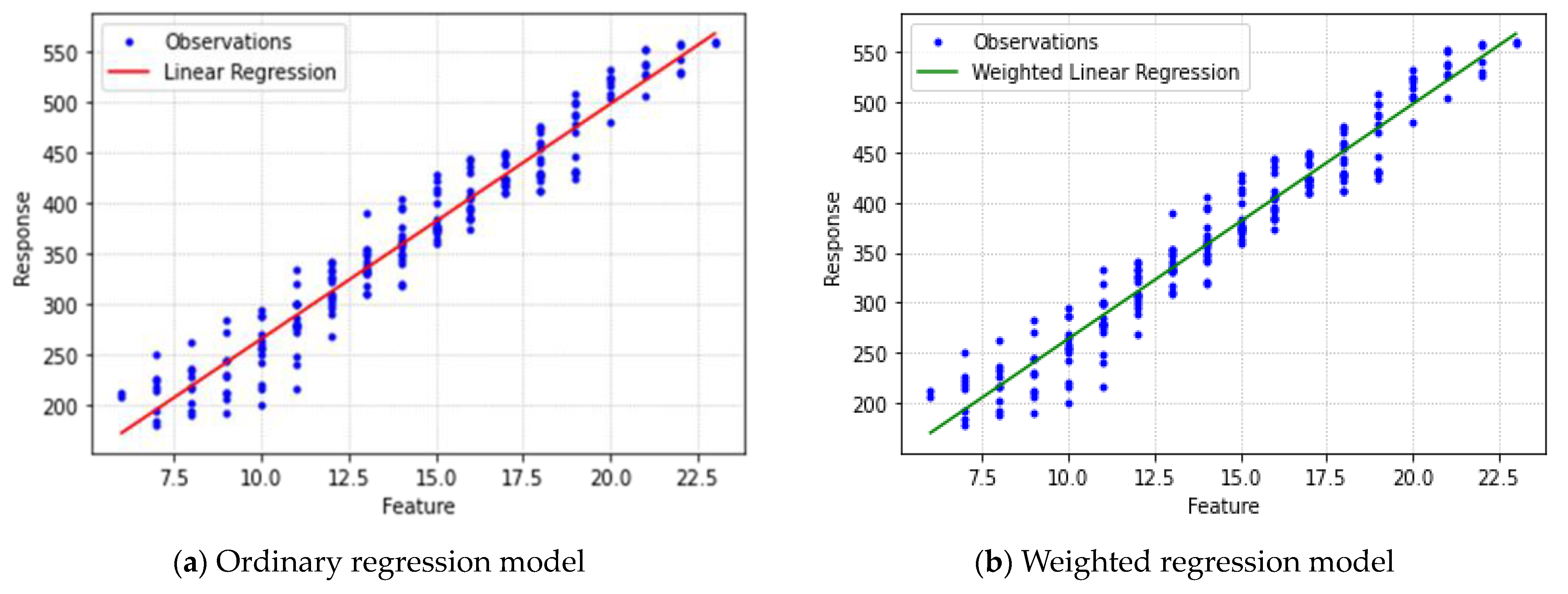
As discussed, in the problem of predicting the weight of Korean cattle, the weight of Hanwoo gradually increases with age, and the variance of weight corresponding to each age also increases. In this case, as a regression model for predicting the weight of Korean cattle, a WRM is appropriate in which the reciprocal of the variance of the response variable corresponding to each measurement point is given as a weight matrix. This approach is suitable because measurements with low variance should be given high weights due to high precision, whereas measurements with significant variances should be given low weights due to low precision. The weight matrix$\mathbf{W}$ is assumed to be a main diagonal matrix in which the main diagonal elements have the variance of each Korean cattle member:

$$\mathbf{W}=\left(\begin{array}{ccc}{w}_1& \cdots & 0\\ ⋮& \ddots & ⋮\\ 0& \cdots & w_N\end{array}\right)=\left(\begin{array}{ccc}2.75& \cdots & 0\\ ⋮& \ddots & ⋮\\ 0& \cdots & 1.0\end{array}\right).$$

Figure 2 illustrates values estimated by the linear regression model and WRM and the actual observed values of the weight of males according to the age of the Korean cattle, expressed as a line.

Figure 2 reveals that it is challenging to visually distinguish the accuracy of the two regression models, so we calculated numerical measures for the two regression models.

Table 3. Performance of ordinary and weighted regression models.

Model	${\mathit{R}}^2$	RMSE	AIC	BIC
Ordinary regression model	0.9424	23.8087	−21.2161	−17.9380
Weighted regression model	0.9424	23.8189	−21.2365	−17.9584

presents the four numerical measures defined above for the ordinary and weighted regression models.

The four measures reveal that the performance of the ordinary regression model and the WRM is almost identical.

3.3.2. Performance of the Gaussian Prosses Regression Model

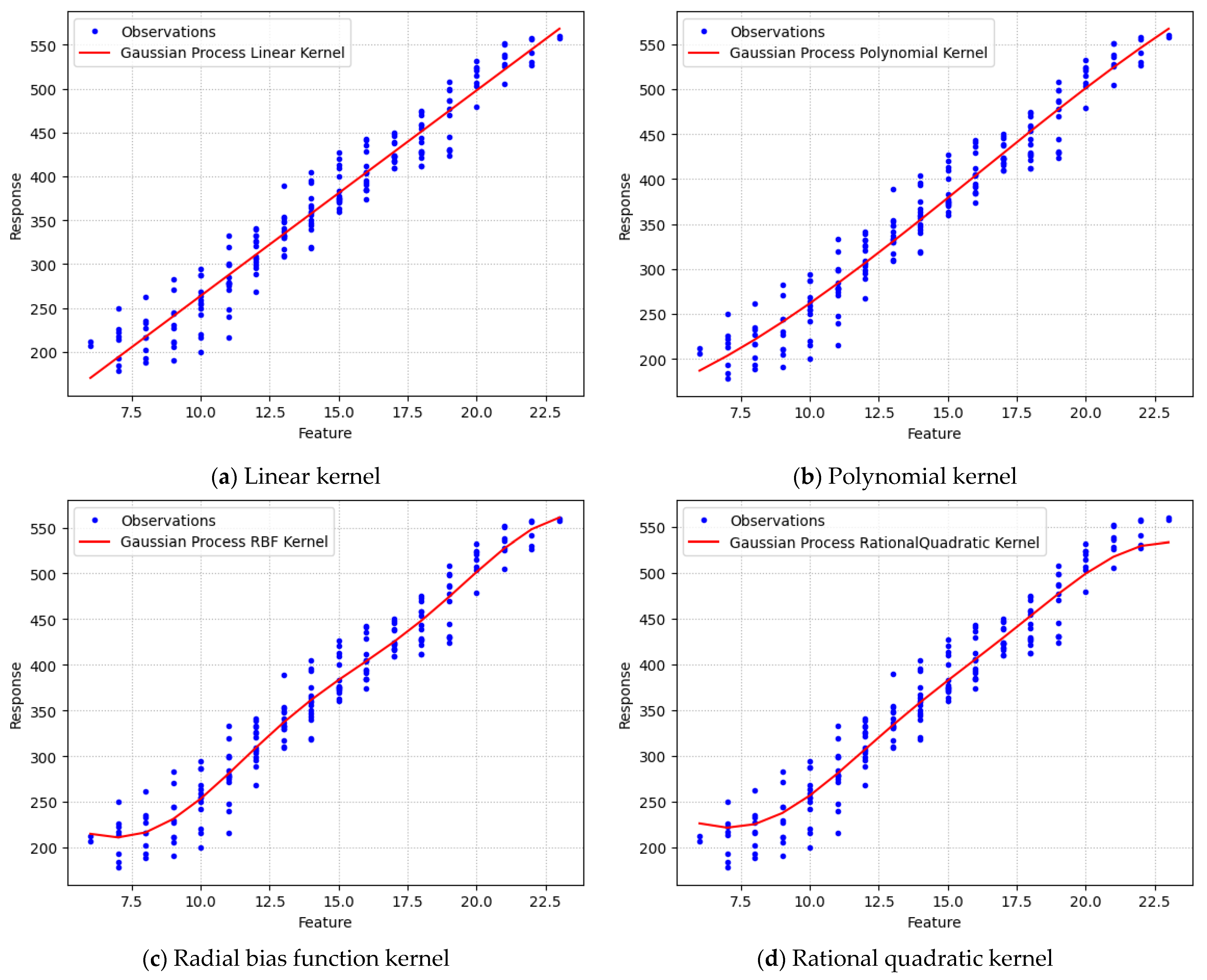
The kernel function generally plays the most crucial role in GPR. The choice of the Gaussian kernel determines almost all of the general properties of the Gaussian process model. We consider four kernel types: linear, polynomial, Gaussian, and rational quadratic, which are defined in

Table 4. Formulas of four kernel functions.

Kernel Function	Formula
Linear kernel	$\mathrm{k}\left(\mathrm{x},x^{\prime }\right)=x·x^{\prime }$
Polynomial kernel	$\mathrm{k}\left(\mathrm{x},x^{\prime }\right)={\left(x·x^{\prime }+a\right)}^b$
Gaussian kernel	$\mathrm{k}\left(\mathrm{x},x^{\prime }\right)={\sigma }^2\exp \left(-\frac{{\left(x-x^{\prime }\right)}^2}{2l^2}\right)$
Rational quadratic kernel	$\mathrm{k}\left(\mathrm{x},x^{\prime }\right)={\sigma }^2{\left(1+\frac{{\left(x-x^{\prime }\right)}^2}{2l^2}\right)}^{-\alpha }$

[31,32].

Each of the four considered kernels is defined through necessary hyperparameters (${\Theta }^{\ast })$, and these parameters are selected to maximize the log marginal likelihood function as follows:

$${\Theta }^{\ast }=\arg \underset{\Theta }{\max }\log p(\mathit{y}|\mathit{X},\Theta ).$$

(30)

Thus, considering the estimated hyperparameters, a more general equation of predictions at the new testing points is given as:

$${\widehat{f}}_{\ast }|X,y,X_{\ast },\Theta ~ \mathcal{N}\left({\overline{f}}_{\ast }, \mathrm{cov}\left(f_{\ast }\right)\right).$$

(31)

After learning and tuning the hyperparameters, the variance of the predictive distribution depends on the inputs $\mathbf{X}$ and ${\mathit{X}}_{\ast }$ and the output $\mathbf{y}$. Finally, the predicted value ${\widehat{f}}_{\ast }$ for the new testing point is given as the mean value ${\overline{f}}_{\ast }$ for the given posterior distribution. We calculated four goodness-of-fit measures to compare the performance of four kernel functions using the given data as shown in Figure 3.

Table 5. Performance comparison of four kernel functions in Gaussian procession regression model.

Kernel Function	${\mathit{R}}^2$	RMSE	AIC	BIC
Linear kernel	0.9396	24.6579	1001.9905	1005.0403
Polynomial kernel	0.9415	24.2580	996.8893	999.9391
Gaussian kernel	0.9464	23.2212	983.2609	986.3108
Rational quadratic kernel	0.9414	24.2709	997.0543	1000.1042

lists the four goodness-of-fit measures for the five kernel functions.

The results of Table 5 indicate that the GPRM with the Gaussian kernel function performs the best, followed by the polynomial and rational quadratic kernels, and the regression model with the linear kernel has the lowest performance.

3.3.3. Performance of the Gaussian Process Panel Model

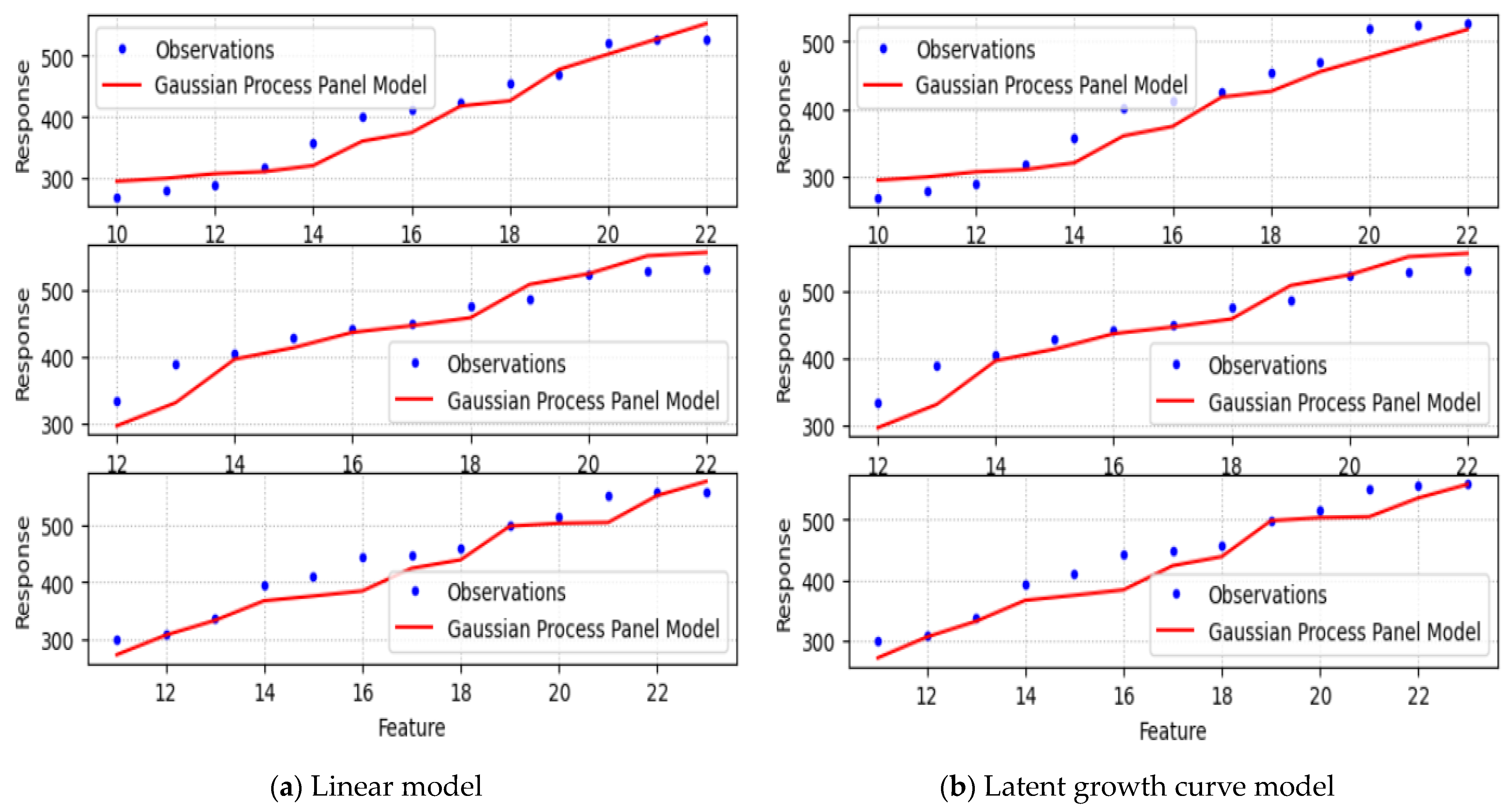
Based on the collected data, we experimented to determine whether GPPM could accurately predict the increase in live weight during the growth period of each member of the Korean cattle. We experimented using the linear model and latent growth curve model (LGCM) used by Karch [27]. The mean function and kernel functions for these two models are given as:

$$\mathrm{Linear} \mathrm{model}: y_i\left({\mathrm{x}}_t\right)~GP\left({\beta }_0+{\beta }_1{\mathrm{x}}_t,\delta \left({\mathrm{x}}_t-{\mathrm{x}}_{t^{\prime }}\right){\sigma }^2\right),$$

(32)

$$\mathrm{LGCM}: a_i ~ \mathcal{N}\left({\mu }_a,{\sigma }_a^2\right), b_i ~ \mathcal{N}\left({\mu }_b,{\sigma }_b^2\right), \mathrm{Cov}\left(a_i,b_i\right)={\sigma }_{ab},$$

(33)

$$y_i\left({\mathrm{x}}_t\right)~GP({\beta }_0+{\beta }_1{\mathrm{x}}_t,{\sigma }_a^2+{\sigma }_{ab}\left({\mathrm{x}}_t+{\mathrm{x}}_{t^{\prime }}\right)+{\mathrm{x}}_t{\sigma }_b^2{\mathrm{x}}_{t^{\prime }}+\delta \left({\mathrm{x}}_t-{\mathrm{x}}_{t^{\prime }}\right){\sigma }^2 ,$$

where $y_i\left(t\right)$ and ${\mathrm{x}}_t$ represent the weight and age of the Korean cattle, respectively. Figure 4 presents the scatterplot of the actual weights of the Korean cattle and the weights predicted by the two models for the three verification datasets. The given scatterplot reveals that both models predict the weight gain of the Korean cattle well during the growing season.

Next, we computed the four measures to quantitatively compare the performance of these two models.

Table 6. Performance comparison of two models with four measures.

Testing Object	Model	${\mathit{R}}^2$	RMSE	AIC	BIC
1	Linear model	0.9291	24.2397	84.8877	85.4527
2		0.8236	25.3405	73.1129	73.5108
3		0.9017	27.5598	88.2253	88.7902
1	LGCM	0.9099	27.3251	88.0030	88.5679
2		0.8236	25.3405	73.1129	73.5108
3		0.9004	27.7333	88.3885	88.9535

displays the computed values of these four measures for both models. Based on the results presented in Table 6, the linear model exhibited better predictive accuracy for the weight of all three individuals, outperforming the LGCM model.

3.4. Summary of the Experimental Results for Three Regression Models

We conducted a comparative experiment for the three models of WRM, GPRM, and GPPM based on observed data to determine which model predicts the weight change well during the growth period of Korean cattle as shown in

Table 7. Comparison of the best performing weighted regression model (WRM), Gaussian process regression model (GPRM), and Gaussian process panel model (GPPM).

Model	${\mathit{R}}^2$	RMSE	AIC	BIC
WRM	0.9424	23.8189	−21.2365	−17.9584
GPRM (Gaussian kernel)	0.9464	23.2212	983.2609	986.3108
GPPM (Linear model)	0.9291	24.2397	84.8877	85.4527

.

In summary, the GPRM with the squared exponential kernel (Gaussian kernel) had the best predictive power for Korean cattle weight. Second, GPRMs with polynomial, rational quadratic, and linear models, and WRMs had the next-best predictive power. Third, the GPRM with the linear kernel, the linear model, and LGCM, and special GPPMs have the next-best predictive power for Korean cattle weight. However, the linear model and LGCM are the results of individually predicting the weight of each member of the Korean cattle. Although the predictive power is poor, this method could be usefully employed in the livestock field in the future.

4. Discussion

This study introduces a prediction system designed to forecast live weight increases during the growth period of livestock raised in farming households. Initially, a linear regression method was proposed for this purpose, followed by the utilization of a growth curve model. In recent times, there has been a surge in studies employing machine learning and deep learning approaches for similar predictions. However, it is important to note that the previously proposed methods have struggled to accurately predict the weight variability of individual livestock.

Among the statistical regression models considered in this study—WRM, GPRM, and GPPM—the latter, GPPM, stands out as a statistical probability model specifically tailored for measuring the weight of individual cattle. It is expected to be highly efficient in predicting the weight of individual cattle on farms, where such precise estimations are crucial. Farm management, particularly when preparing cattle for shipment, often requires individual-level attention. Consequently, GPPM is regarded as a practical and widely applicable method on farms, facilitating precise predictions of individual cattle weights and enhancing overall management and production efficiency.

5. Conclusions

This study has developed a GPPM with a primary focus on predicting the weight of individual cattle, emphasizing its potential to significantly support individual cattle management and facilitate shipment procedures on farms. As we look to the future, our research endeavors will involve enhancing the predictive capabilities of the proposed regression models by collecting diverse cattle weight-related data from additional livestock farms. Moreover, we plan to extend the applicability of the developed prediction model to other livestock species, such as cows, pigs, and sheep, without confining it exclusively to Korean cattle.

References

- Wang, Z.; Shadpour, S.; Chan, E.; Rotondo, V.; Wood, K.M.; Tulpan, D. ASAS-NANP Symposium: Applications of machine learning for livestock body weight prediction from digital images. J. Anim. Sci. 2021, 99, skab022. [Google Scholar] [CrossRef] [PubMed]
- Dohmen, R.; Catal, C.; Liu, Q. Computer vision-based weight estimation of livestock: A systematic literature review. N. Z. J. Agric. Res. 2021, 65, 227–247. [Google Scholar] [CrossRef]
- Sanotra, G.S.; Lund, J.D.; Ersøll, A.K.; Petersen, J.S.K.; Vestergaard, S. Monitoring leg problems in broilers: A survey of commercial broiler production in Denmark. Worlds Poult. Sci. J. 2001, 57, 55–69. [Google Scholar] [CrossRef]
- Ruchay, A.N.; Kober, V.; Dorofeev, K.; Kolpakov, V.; Gladkov, A.; Guo, H. Live Weight Prediction of Cattle Based on Deep Regression of RGB-D Images. Agriculture 2022, 12, 1794. [Google Scholar] [CrossRef]
- Yan, T.; Mayne, C.S.; Patterson, D.C.; Agnew, R.E. Prediction of body weight and empty body composition using body size measurements in lactating dairy cows. Livest. Sci. 2009, 124, 233–241. [Google Scholar] [CrossRef]
- Tasdemir, S.; Urkmez, A.; Inal, S. Determination of body measurements on the Holstein cows using digital image analysis and estimation of live weight with regression analysis. Comput. Electron. Agric. 2011, 76, 189–197. [Google Scholar] [CrossRef]
- Gruber, L.; Ledinek, M.; Steininger, F.; Fuerst-Waltl, B.; Zottl, K.; Royer, M.; Krimberger, K.; Mayerhofer, M.; Egger-Danner, C. Body weight prediction using body size measurements in Fleckvieh, Holstein, and Brown Swiss dairy cows in lactation and dry periods. Arch. Anim. Breed. 2018, 61, 413–424. [Google Scholar] [CrossRef]
- Vanvanhossou, S.F.U.; Diogo, R.V.C.; Dossa, L.H. Estimation of live bodyweight from linear body measurements and body condition score in the West African Savannah Shorthorn cattle in North-West Benin. Cogent Food Agric. 2018, 4, 1549767. [Google Scholar] [CrossRef]
- de Moraes Weber, V.A.; de Lima Weber, F.; da Costa Gomes, R.; da Silva Oliveira, A., Jr.; Menezes, G.V.; de Abreu, U.G.P.; de Souza Belete, N.A.; Pistori, H. Prediction of Girolando cattle weight by means of body measurements extracted from images. Braz. J. Anim. Sci. 2020, 49, 1–12. [Google Scholar]
- Luo, J.; Lei, H.; Shen, L.; Yang, R.; Pu, Q.; Zhu, K.; Li, M.; Tang, G.; Li, X.; Zhang, S.; et al. Estimation of Growth Curves and Suitable Slaughter Weight of the Liangshan Pig. Asian Australas. J. Anim. Sci. 2015, 28, 1252–1258. [Google Scholar] [CrossRef]
- Widyas, N.; Prastowo, S.; Widi, T.S.M.; Baliarti, E. Predicting Madura cattle growth curve using non-linear model. IOP Conf. Ser. Earth Environ. Sci. 2018, 142, 012006. [Google Scholar] [CrossRef]
- Fernandes, F.A.; Fernandes, T.J.; Pereira, A.A.; Meirelles, S.L.C.; Costa, A.C. Growth curves of meat-producing mammals by von Bertalanffy’s model. Pesqui. Agropecuária Bras. 2019, 54, 1–8. [Google Scholar] [CrossRef]
- Onogi, A.; Ogino, A.; Sato, A.; Kurogi, K.; Yasumori, T.; Togash, K. Development of a structural growth curve model that considers the causal effect of initial phenotypes. Genet. Sel. Evol. 2019, 51, 19. [Google Scholar] [CrossRef]
- Do, D.N.; Miar, Y. Evaluation of Growth Curve Models for Body Weight in American Mink. Animals 2020, 10, 22. [Google Scholar] [CrossRef] [PubMed]
- Hartati, H.; Putra, W.P.B. Predicting the growth curve of body weight in Madura Cattle. Kafkas Univ. Vet. Fak. Derg. 2021, 27, 431–437. [Google Scholar]
- Adinata, Y.; Noor, R.R.; Priyanto, R.; Sudrajad, P. Comparison of Growth Curve Models for Ongole Grade Cattle. Res. Sq. 2022, 54, 252. [Google Scholar] [CrossRef]
- Miller, G.A.; Hyslop, J.J.; Barclay, D.; Edwards, A.; Thomson, W.; Duthie, C.-A. Using 3D Imaging and Machine Learning to Predict Live Weight and Carcass Characteristics of Live Finishing Beef Cattle. Front. Sustain. Food Syst. 2019, 3, 30. [Google Scholar] [CrossRef]
- Cozler, Y.L.; Allain, C.; Xavier, C.; Depuille, L.; Caillot, A.; Delouard, J.M.; Delattre, L.; Luginbuhl, T.; Faverdin, P. Volume and surface area of Holstein dairy cows calculated from complete 3D shapes acquired using a high-precision scanning system: Interest for body weight estimation. Comput. Electron. Agric. 2019, 165, 104977. [Google Scholar] [CrossRef]
- Ruchay, A.N.; Kolpakov, V.I.; Kalschikov, V.V.; Dzhulamanov, K.M.; Dorofeev, K.A. Predicting the body weight of Hereford cows using machine learning. IOP Conf. Ser. Earth Environ. Sci. 2021, 624, 012056. [Google Scholar] [CrossRef]
- Ruchay, A.N.; Kober, V.; Dorofeev, K.; Kolpakov, V.; Dzhulamanov, K.; Kalschikpv, V.; Guo, H. Comparative analysis of machine learning algorithms for predicting live weight of Hereford cows. Comput. Electron. Agric. 2022, 195, 106837. [Google Scholar] [CrossRef]
- Na, M.-H.; Cho, W.H.; Kim, S.K.; Na, I.S. Automatic Weight Prediction System for Korean Cattle Using Bayesian Ridge Algorithm on RGB-D Image. Electronics 2022, 11, 1663. [Google Scholar] [CrossRef]
- Gebreyesus, G.; Milkevych, V.; Lassen, J.; Sahana, G. Supervised learning techniques for dairy cattle body weight prediction from 3D digital images. Front. Genet. 2023, 13, 947176. [Google Scholar] [CrossRef] [PubMed]
- Guvenoglu, E. Determination of the Live Weight of Farm Animals with Deep Learning and Semantic Segmentation Techniques. Appl. Sci. 2023, 13, 6944. [Google Scholar] [CrossRef]
- Oliveira, D.A.B.; Pereira, L.G.R.; Bresolin, T.; Ferreira, R.E.P.; Dorea, J.R.R. A review of deep learning algorithms for computer vision systems in livestock. Livest. Sci. 2021, 253, 104700. [Google Scholar] [CrossRef]
- Rasmussen, C.E.; Christopher, K.I.; Williams, C.K.I. Gaussian Processes for Machine Learning; MIT Press: Cambridge, MA, USA, 2006. [Google Scholar]
- Karch, J.D.; Brandmaier, A.M.; Voelkle, M.C. Gaussian Process Panel Modeling—Machine Learning Inspired Analysis of Longitudinal Panel Data. Front. Psychol. 2020, 11, 351. [Google Scholar] [CrossRef]
- Karch, J.D. A Machine Learning Perspective on Repeated Measures: Gaussian Process Panel and Person-Specific EEG Modeling. Ph.D. Thesis, Humboldt-Universitat, Berlin/Heidelberg, Germany, 2016. [Google Scholar]
- Chen, Y.; Prati, A.; Montgomery, J.; Garnet, R. A Multi-Task Gaussian Process Panel Modeling—Machine Learning Inspired Analysis of Longitudinal Panel Data. In Proceedings of the 26th International Conference on Artificial Intelligence and Statistics (AISTATS), Valencia, Spain, 25–27 April 2023; Volume 206, pp. 1–21. [Google Scholar]
- Korean Livestock Act Enforcement Regulation [Presidential Decree No. 32692, 14 June 2022, Partial Amendment].
- Lohr, S.L. Sampling Design and Analysis, 3rd ed.; Chapman & Hall: London, UK, 2021; ISBN 9780367279509. [Google Scholar]
- Chen, Z.; Wang, B. How priors of initial hyperparameters affect Gaussian process regression models. Neurocomputing 2018, 275, 1701–1710. [Google Scholar] [CrossRef]
- Duvenaud, D. The Kernel Cookbook. Available online: httpe://www.cs.toronto.edu/~duvenaud/cookbook (accessed on 17 September 2023).
Figure 1.
Weight distribution of each Korean cattle member: each cattle member is represented by a different color.
Figure 2.
Estimated regression using the ordinary and weighted regression models.
Figure 3.
Comparison for four kernel functions in Gaussian procession regression model.
Figure 4.
Comparison of Gaussian process panel models (linear and latent growth curve models).