
An Aquatic Product Price Forecast Model Using VMD-IBES-LSTM Hybrid Approach


College of Economics and Management, Shanghai Ocean University, Shanghai 201306, China
*
Author to whom correspondence should be addressed.
Agriculture 2022, 12(8), 1185; https://doi.org/10.3390/agriculture12081185
Submission received: 26 June 2022
/
Revised: 26 July 2022
/
Accepted: 27 July 2022
/
Published: 9 August 2022
(This article belongs to the Special Issue Internet and Computers for Agriculture)
Abstract
:Changes in the consumption price of aquatic products will affect demand and fishermen’s income. The accurate prediction of consumer price index provides important information regarding the aquatic product market. Based on the non-linear and non-smooth characteristics of fishery product price series, this paper innovatively proposes a fishery product price forecasting model that is based on Variational Modal Decomposition and Improved bald eagle search algorithm optimized Long Short Term Memory Network (VMD-IBES-LSTM). Empirical analysis was conducted using fish price data from the Department of Marketing and Informatization of the Ministry of Agriculture and Rural Affairs of China. The proposed model in this study was subsequently compared with common forecasting models such as VMD-LSTM and SSA-LSTM. The research results show that the VMD-IBES-LSTM model that was constructed in this paper has good fitting results and high prediction accuracy, which can better explain the seasonality and trends of the change of China’s aquatic product consumer price index, provide a scientific and effective method for relevant management departments and units to predict the aquatic product consumer price, and have a certain reference value for reasonably coping with the fluctuation of China’s aquatic product market price.
1. Introduction
Aquatic products play an important role in China’s fishery economic development and international market competition. As a specific reflection of the fishery production cost and the relationship between the supply and demand of aquatic products, aquatic product price is not only related to the production and sales of enterprises and economic interests, but also related to China’s macroeconomic policies. In recent years, with the rapid development of China’s economy and the continuous advancement of urbanization, residents’ demand for high-quality and safe aquatic products such as abalone and shark fin has gradually increased [1,2,3]. Meanwhile, China’s aquatic product market structure is increasingly in line with the needs of the world [4]. The accurate forecast of aquatic product price can make aquiculturists understand the changing trend of market in time, and then rationally plan the aquaculture structure, and realize the maximization of aquaculture benefits. At the same time, the price forecast provides a scientific basis for the government to make relevant industry policies, and strive to make full use of resources and promote the healthy and sustainable development of aquaculture. In addition, the price of aquatic products can also play a certain reference role in consumers’ choice.
This study takes the prices of five common fishery products, including crucian carp, grass carp, and carp, as the object of study. The reasons are shown below. Changes in aquatic product prices affect a large number of Chinese people. According to the China Fisheries Economic Statistics Bulletin for 2021, in 2021, the value of fishery output was 224347.724 million dollars, accounting for 51.1% of China’s total annual fishery economic output. Secondly, the total population that was engaged in fishery fishing was 16,342,400. However, in other countries, due to the relatively small proportion of people that are engaged in fishing, the impact of price changes on fishermen is relatively small. Therefore, it is very necessary to establish the prediction model of aquatic product price.
The innovations in this paper are shown below (1) Introducing variational modal decomposition (VMD), which has great advantages in dealing with non-stationary and non-linear time series [5]. The VMD model can decompose the original time series into several sub-series, which enlarges the details in the time series data and makes the fluctuation of sub-series smoother than the original series, which can improve the prediction accuracy of each decomposed sub-model. Therefore, this study introduced variational modal decomposition to decompose the fish price series in order to improve the accuracy of the model. (2) Based on the characteristics that the bald eagle search optimization algorithm has strong optimization-seeking ability and requires fewer parameters to be set, but easily falls into local optimality, levy flight and Tent mapping are introduced to improve the bald eagle search algorithm, and the improved bald eagle search optimization algorithm is utilized to optimize the parameters of the long short-term memory network(LSTM) to improve the accuracy of the model. (3) A comparison with common prediction models was made and the outcome indicated that compared with other popular prediction models, the RMSEs of the VMD-IBES-LSTM model that was proposed in this paper on the five fish price test sets are 0.480, 0.214, 0.288, 0.58, and 0.68, respectively, which is much lower than other models.
2. Literature Review
Scholars have proposed a large number of methods for price prediction. Huang et al. [6] used coal prices, which are highly non-linear and non-stationary, as the subject of their study. First, VMD was used to decompose the coal price dataset. Subsequently, GARCH and LSTM models were used to forecast each IMF component, respectively. The results show that the model has the smallest error compared to other econometric and deep-learning models. Lin et al. [7] constructed a VMD-AR-IBILSTM-ELMAN model using the prices of gas and coal from 1 December 2009 to 30 November 2020 as the study object. Subsequently, it was compared with 16 models such as GRU, VMD-GRU, and others, and the outcome indicated that the MSE of the VMD-AR-IBILSTM-ELMAN model on the gasoline and coal price datasets was 0.0106 and 0.649, respectively, which was much lower than the other models. Sun et al. [8] developed an EMD-VMD-LSTM model using the carbon prices of eight carbon markets in China, including Beijing and Fujian, as the object of study. First, EMD was used to decompose the carbon price dataset into a number of IMF components. Subsequently, based on the high volatility of IMF1, VMD was used to perform a secondary decomposition of IMF1. Finally, LSTM was introduced to forecast the individual IMF components. The results show that the robustness and accuracy of the model is optimal compared to EMD-LSTM, LSTM and other models. Liang et al. [9] constructed an ICEEMDAN-LSTM-CNN-CBAM model using the price of gold as the object of study. First, ICEEMDAN was used to decompose the gold price dataset into individual IMF components, and subsequently, the LSTM-CNN-CBAM model was used to forecast the individual IMF components. Ultimately, the ICEEMDAN-LSTM-CNN-CBAM model is compared with 11 common models such as LSTM and CNN-LSTM. The outcome indicated that the accuracy of the models is greatly improved after the signal processing approach is adopted. In addition, the accuracy of the ICEEMDAN-LSTM-CNN-CBAM model is significantly better than the other models. Huang et al. [10] constructed a VMD-LSTM-MW model using crude oil prices from January 1994 to July 2018 as the study object and subsequently compared it with ELM, ARIMA, and other models. The results showed that the MAPE of the VMD-LSTM-MW model was 0.46, which was much lower than the other models. Liu et al. [11] constructed a VMD-LSTM model using the non-ferrous metal prices for each trading day from 2 June 2006 to 21 March 2019 as the study object. First, VMD was used to decompose it into a number of IMF components. Subsequently, each IMF component was used as an input to the LSTM and the test set was predicted. The outcome showed that the RMSEs of the VMD-LSTM model on the zinc, copper, and aluminum price datasets are 4.79, 7.48, and 2.83, respectively, which are much lower than those of the ARIMA and LSTM models. Rezaei et al. [12] constructed CEEMD-CNN-LSTM and EMD-CNN-LSTM models using four groups of stock prices from January 201 to September 2019 as the subjects of their study. The results indicated that the CEEMD-CNN-LSTM outperformed the other models in terms of accuracy.
Aquatic products are a crucial component of agricultural products and the fluctuation of aquatic product price is characterized by nonlinear, non-stationary, and periodicity [13]. Its price forecasting research is less explored compared to other agricultural products. Nam and Sim [14] proposed an ARMA model with different parameters based on the price of abalone with different shell sizes and then used Diebold–Mariano to test the model. The test results indicated an increase in the accuracy of the improvement. Mustapa et al. [15] used an autoregressive integrated moving average model (ARIMA) to predict the prices of ten kinds of fish and vegetables in Malaysia based on data from the network. Hasan et al. [16] used the ARIMAX model to forecast catfish prices and the results indicated that the model has high predictive accuracy for both in-sample and out-of-sample. Gordon [17] used the ARDL/Bounds model to forecast lobster prices. Guillen et al. [18] used the Hedonic model to analyze eight aquatic products (e.g., cod, red mullet, flounder, etc.) in Spain from 2000 to 2013 and the results showed that the prices of aquatic products depend on the economic cycle. Khanh Nguyen et al. [19] used the ARIMAX model to forecast the price of catfish based on the uncertainty of the profitability of the catfish industry. They concluded that Vietnam people have laid little attention to the need for a sustainable and comprehensive action plan for animal-based aquatic product exports. This could have negative impacts on many aspects such as the environment and the economy.
In recent years, with the rapid development of machine learning technology, scholars have gradually applied various machine learning techniques to fish price prediction. Li Hongwei et al. [20] used wavelet function to replace the excitation function in the BP neural network to predict the price of perch and validated the model with three fish prices in ULUNGU lake. Duan, et al. [21] used the genetic algorithm to optimize the SVR model and predicted the prices of fish such as Mandarin Fish. The model was then compared with the BP neural network model and the SVR model. The results proved that the prediction accuracy of the model was significantly improved and superior compared to other models. Bloznelis [22] selected ARIMA, ANN, and KNN models to predict the price of salmon. The results showed that KNN had the highest prediction accuracy for salmon prices.
In summary, although there has been much research for price prediction [23,24], laying the foundation for this study, there is still room for further improvement: (1) A single prediction method is easily affected by the fluctuation of fish price series, resulting in lower prediction accuracy. (2) The selection of model parameters, such as the number of nodes in the implicit layer, the number of training times, and the initial learning rate in the long short-term memory network (LSTM), will have a great impact on the fitting ability of the model, and an unreasonable setting of parameters will not lead to satisfactory prediction results.
The rest of this paper is organized as follows. In Section 3, We introduce variational modal decomposition (VMD), bald eagle search algorithm (BES), improved bald eagle search optimization algorithm (IBES), long short-term memory network (LSTM), VMD-IBES-LSTM model framework, and the evaluation index criterion. In Section 4, the results of the numerical experiments are analyzed and compared with the relevant literature and also the reasons for the similarities and differences are discussed. Finally, conclusions and future research directions are given in Section 5.
3. Materials and Methods
3.1. Variational Modal Decomposition
Variational modal decomposition (VMD) is a new adaptive signal decomposition method that was proposed by Dragomiretskiy et al. [25]. It works by decomposing a multi-component signal into multiple single-component AMF signals, and then decomposing the original signal into several IMF components by solving a constrained variational problem, which has powerful non-linear and non-smooth signal processing capability. It can minimize the impact of fish price data on the prediction results due to high volatility and strong nonlinearity, etc. Compared with other decomposition methods such as EEMD, it can also solve the residual noise problem.
3.2. Bald Eagle Search Algorithm (BES)
Malaysian scholars proposed the BES algorithm in 2020 [26], which is a novel meta-heuristic algorithm with strong optimal solution search capability, and thus has received extensive research and attention from scholars in various countries. The algorithm simulates the predation behavior of bald eagles on salmon. In the process of predation on salmon, the bald eagle will firstly select a search space based on the distance of individuals and populations to salmon, flying towards a specific area; secondly, they search the water within the selected search space until a suitable prey is found; and finally the bald eagle will gradually change the altitude of its flight and dive downwards rapidly to successfully capture a prey item such as salmon from the water.
The bald eagle search algorithm is modeled on the behavior of a bald eagle hunting for prey in three stages:
- Select the search space.
The bald eagle randomly selects an area to search and subsequently makes a judgement about the number of prey items to find the best location. The equation for updating a bald eagle’s position is:
In the Equation (1), is the best position that is determined by the current bald eagle search down. is the average position of the bald eagle at the end of the previous search. r is a random number between 0 and 1, and is the parameter, which takes values in the range 1.5 to 2.
- Search for prey in a selected space.
To speed up the search process to find the prey, the bald eagle flies in a spiral form, so the polar equation of the spiral is adopted here for the position update. The relevant equation is shown below:
where is the polar angle of the spiral equation, is the polar diameter of the spiral equation, , are both parameters controlling the trajectory of the spiral, the ranges of variation are ,, , and are the position of the bald eagle in polar coordinates, the range of values are , The formula for updating the location of the bald eagle is shown below:
- Swoop to capture prey.
After the first and second steps, the bald eagle swoops from its optimal position towards its target. This is still represented here using the polar equation:
During the dive, the equation for updating the position of the bald eagle is:
where: c1 denotes the intensity of the bald eagle’s movement towards the optimal position and c2 denotes the intensity of the bald eagle’s movement towards the central position. The range of c1 and c2 is between 1 and 2.
3.3. Improved Bald Eagle Search Algorithm (IBES)
To address the problem that the bald eagle search algorithm is prone to slow convergence and falls easily into local optima when dealing with problems [20], the overall performance of the Bald eagle search algorithm is improved by two main strategies.
- (1)
- Population initialization strategy based on Tent mapping.
The more uniformly the initial population is distributed in the search space, the more beneficial it is to improve the algorithm’s optimization-seeking efficiency and the accuracy of the solution [27,28,29]. The initialized population of the traditional bald eagle search algorithm is randomly generated, which cannot guarantee that the initial population individuals are uniformly distributed in the solution space, and the over-concentration of the population may result in local optimality. Chaotic sequences have better randomness, regularity as well as ergodicity. Compared with other mappings, the Tent mapping generates a more balanced distribution of sequences. the expression of the Tent mapping is:
The most uniform distribution series can be produced when u = 0.5. The distribution density at this point is insensitive to changes in the parameters, which is the most typical Tent mapping. The formula is:
The equation for population X is shown below:
where: Xmax and Xmin are the upper and lower bound of the search, respectively.
- (2)
- Local search strategy based on levy flight.
Levy flight was proposed by P. Levy in 1937, initially to describe the activity of a population of organisms. Through the study of the wandering foraging behavior of a population of organisms, a Levy flight with a combination of long and short distance jumps was gradually formed. Levy flight has been widely used in many fields. The position update formula of Levy flight is:
where: α is the random step size, ⊕ is the dot product, Levy is the random search path that fits the Levy distribution and meets the following constraints:
where: u and v follow standard normal distribution and λ = 1.5:
The steps of the improved bald eagle search algorithm are shown below:
- Set the parameters of the algorithm. The parameters that are initially set are mainly the number of populations, the maximum number of iterations T, the dimension D, the upper limit UB, and the lower limit LB of the solution space.
- Initialize the population using the Tent mapping strategy, the maximum number of iterations and other parameters.
- Calculate the fitness values and rank them.
- Select the search space.
- Search for prey in the selected space.
- Swoop to capture prey.
- Calculate fitness values and update bald eagle position.
- Calculate the inertia weighting factors and use roulette wheel selection to levy flight variation on the selected individual sparrows.
- Determine whether the stopping condition is satisfied. Exit and output the results if the stopping condition is met, otherwise, repeat Steps 2–9.
3.4. LSTM
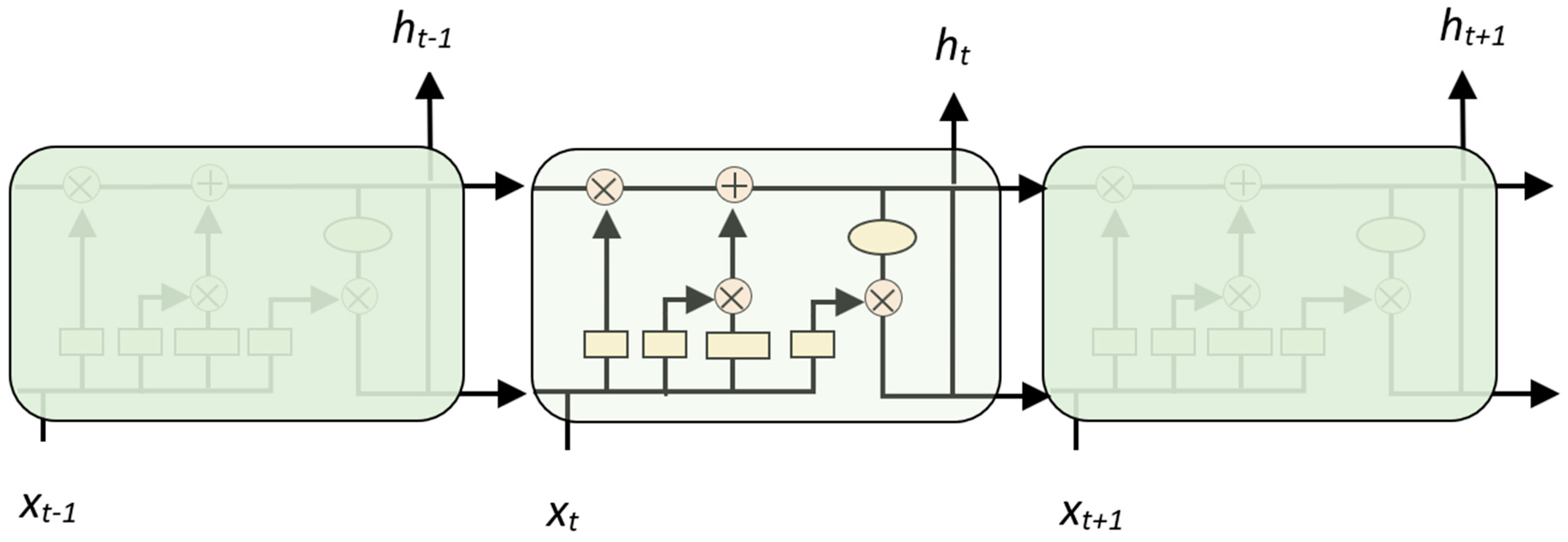
Recurrent neural networks were introduced in the 1980s, as a popular algorithm in deep-learning. Compared to deep-learning networks (DNNs), their recurrent network structure allows them to make full use of the sequence information in the sequence data itself, and, therefore, have many advantages in dealing with time series, and the ability to correct errors that is achieved through back propagation and gradient descent algorithms. However, there are also many problems such as gradient disappearance or gradient explosion due to the increase in the number of network layers with time. Therefore, Hochreiter et al. [30] proposed a long-short term memory network in 1997. Figure 1 shows the topology of a long-short term memory network.
Unlike traditional recurrent neural networks that rewrite memories at each time step, LSTMs save the important features that they learn as long-term memories and selectively retain, update, or forget the saved long-term memories according to the learning process, while features that are always given little weight in multiple iterations are considered short-term memories and are eventually forgotten by the network. This mechanism allows important feature information to be passed on over iterations, allowing the network to perform better in classification tasks with long-dependent samples. In recent years, LSTM has been applied extensively in time series prediction [31,32,33], predicting key parameters of nuclear power plants [34], wind speed prediction [35,36], financial price trends [37], language processing [38], etc. The LSTM model has made a series of improvements on the basis of RNN neurons. It adds a transmission unit state in the RNN hidden layer and is controlled by three gating units: forgetting gate, input gate, and output gate.
3.5. Hybrid Model of Aquatic Products Prices Forecasting
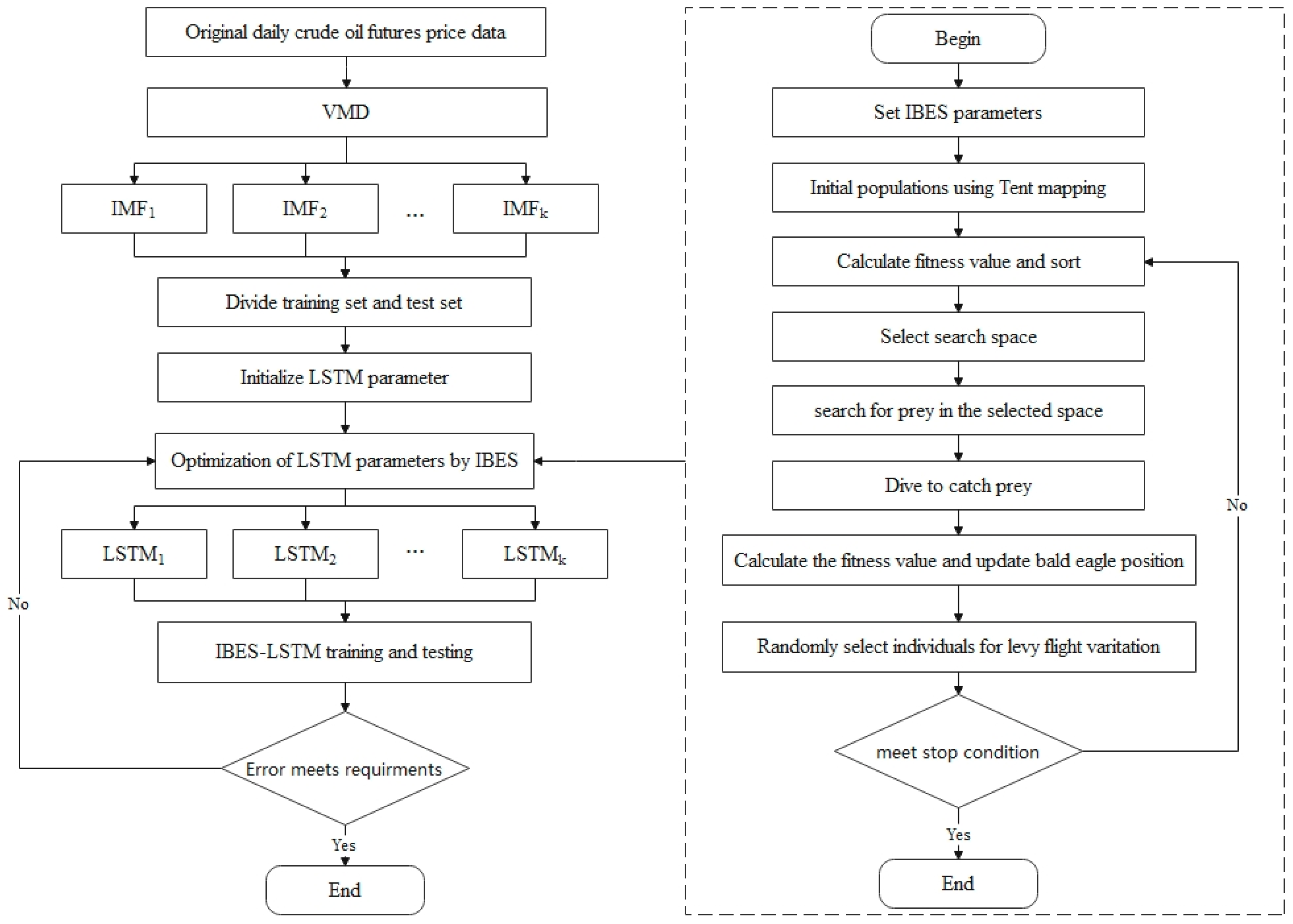
The model that is proposed in this study is divided into four main parts as follows
- The data pre-processing stage. First, the original aquatic product time series with strong non-linearity is decomposed into a series of IMF components using variational modal decomposition.
- Optimization based on IBES. The time window step, the number of hidden layer units, the learning rate and the number of training times in the LSTM model are used as the optimization objects of the improved bald eagle search algorithm, and the parameters of the IBES algorithm (maximum number of iterations, number of populations, upper limit, lower limit, etc.) are initialized.
- Use the hybrid model to do prediction and evaluation. The LSTM network model is constructed using the optimal time window step, number of hidden layer units, learning rate and training times, and the model is trained and subsequently predicted for the test set.
- The prediction results that are obtained from the sub-series test set are added by simple linear summation to obtain the final prediction results. The flow chat is shown below (Figure 2).
3.6. Error Evaluation Criteria
In this study, four metrics, namely mean square error (MSE), root mean square error (RMSE), mean absolute error (MAE), and mean percentage error (MAPE), are chosen as the basis for judging the predictive performance of the model. MAE is used to measure the mean absolute error between the predicted and actual values. RMSE is used to measure the deviation between the predicted and actual values, which is sensitive to outliers, while MAPE is used to measure the average relative error between the predicted and actual values. The formulae for calculating each indicator are shown below:
4. Computational Experiments and Analyses
4.1. Data Source and Descriptive Analysis
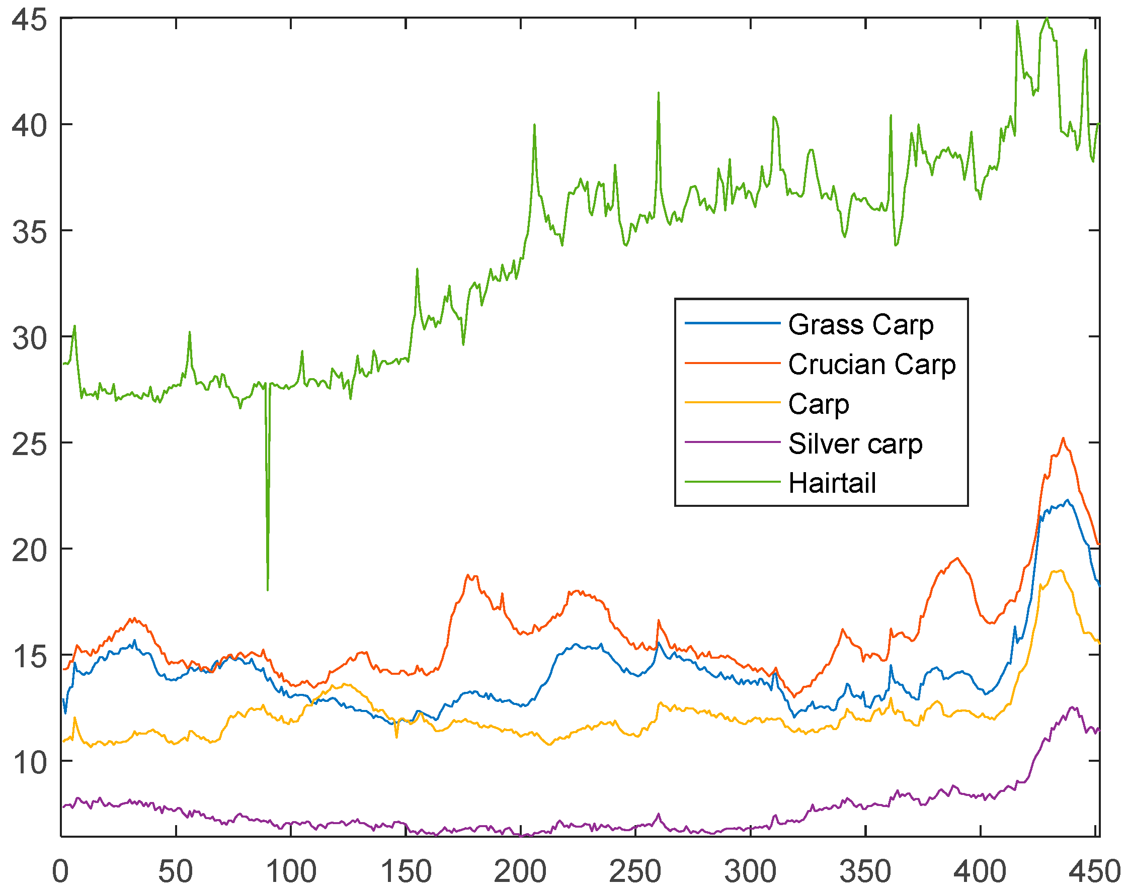
In this study, five common aquatic products, grass carp, crucian carp, carp, white chub, and big scallop were selected as the research objects. The time was from the 52nd week of 2012 to the 44th week of 2021. The data update cycle was once a week, with a total of 452 groups of data. The data are mainly from the market and Information Department of the Ministry of Agriculture and Rural Areas of China. The images of each dataset are shown below (Figure 3).
This paper first used SPSS26 software (Armonk, NY, USA) to conduct descriptive statistics on the data and the results are shown in Table 1.
The Pearson correlation coefficient was then measured using SPSS26 software to screen the input data for the prediction model and determine the correlation results between the different data (Table 2).
4.2. VMD Results
In the VMD parameters, if the K value is too small, some important information of the original data may be ignored, resulting in insufficient prediction accuracy. If the K value is too large, the central frequencies of neighboring modal components may be close to each other, which may lead to problems such as mode repetition or the generation of additional noise, adversely affecting the achievement of high prediction accuracy. Therefore, it is crucial to determine the correct value of the modal number k. In this paper, to determine the k-value, the original data is first automatically decomposed into multiple modes by EMD, and then the K-value is determined according to the number of modes that are decomposed by the EMD algorithm adaptively. This method can effectively improve the efficiency of parameter selection [39,40,41].
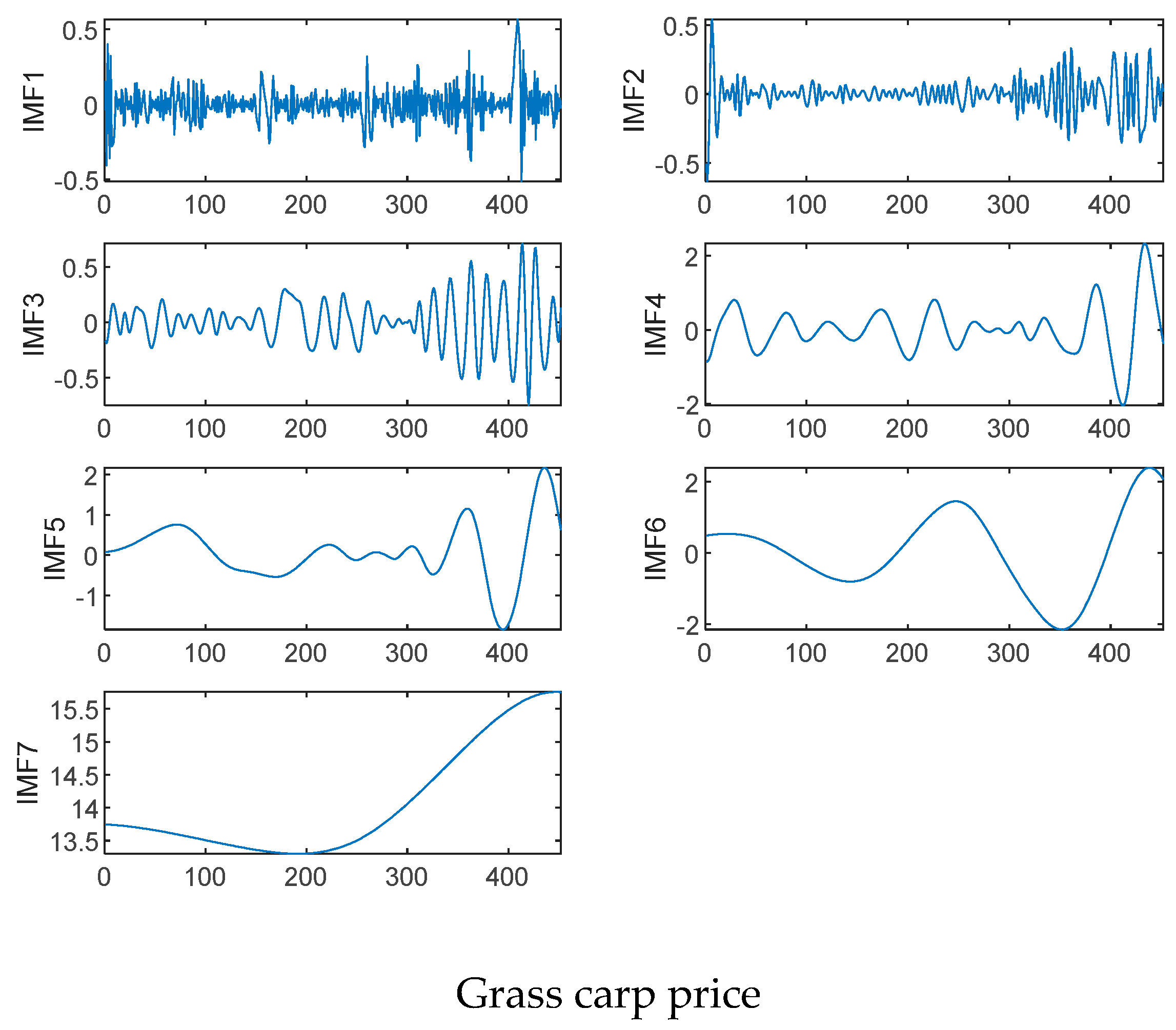
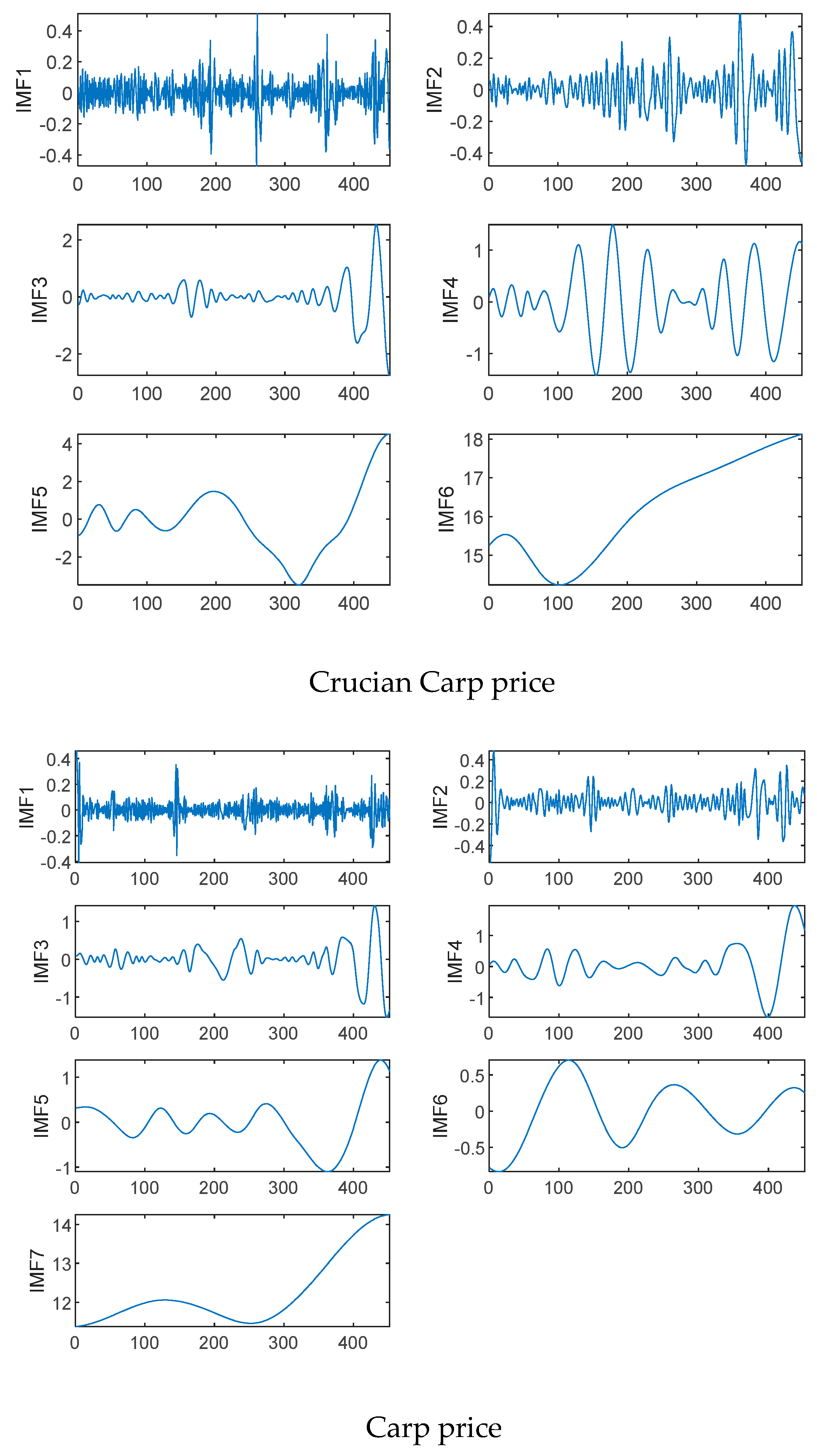
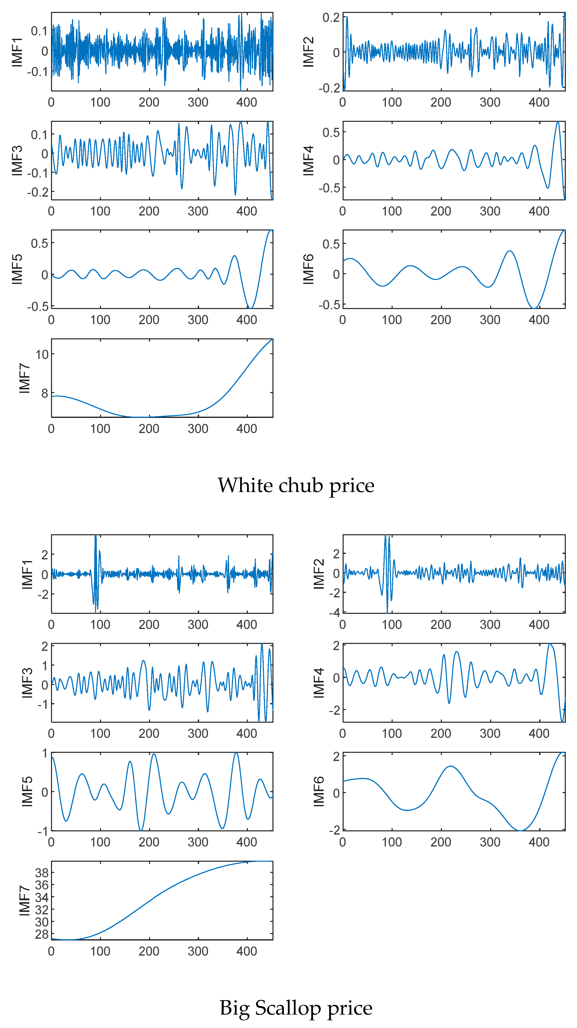
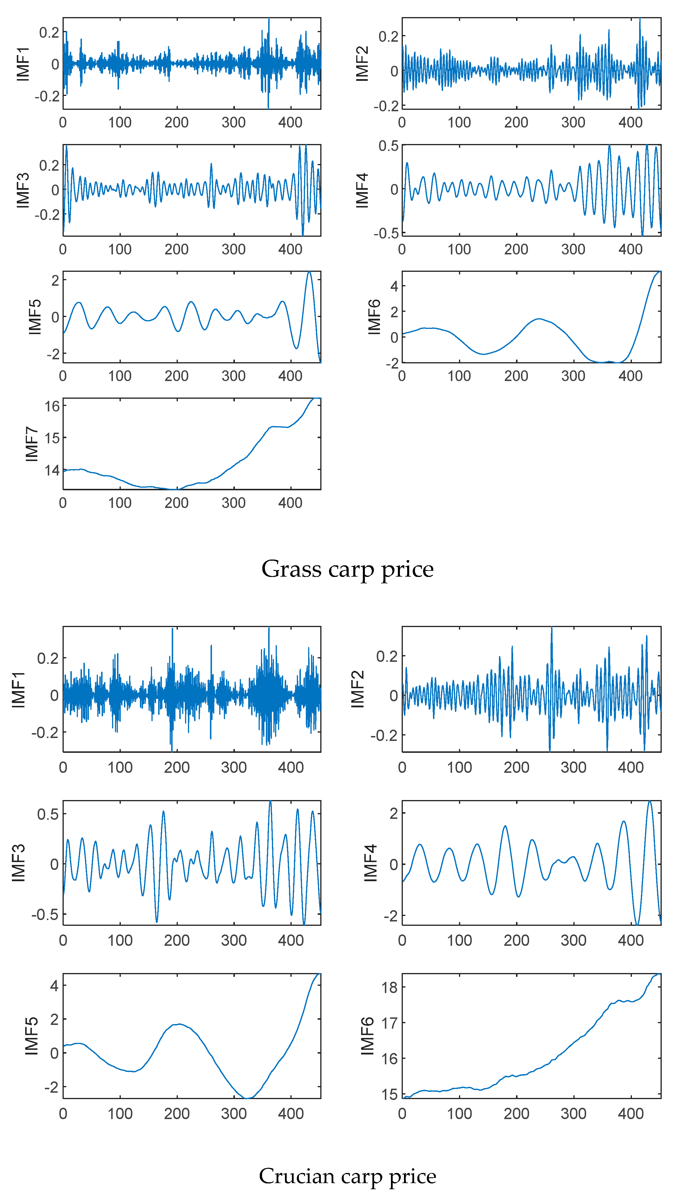
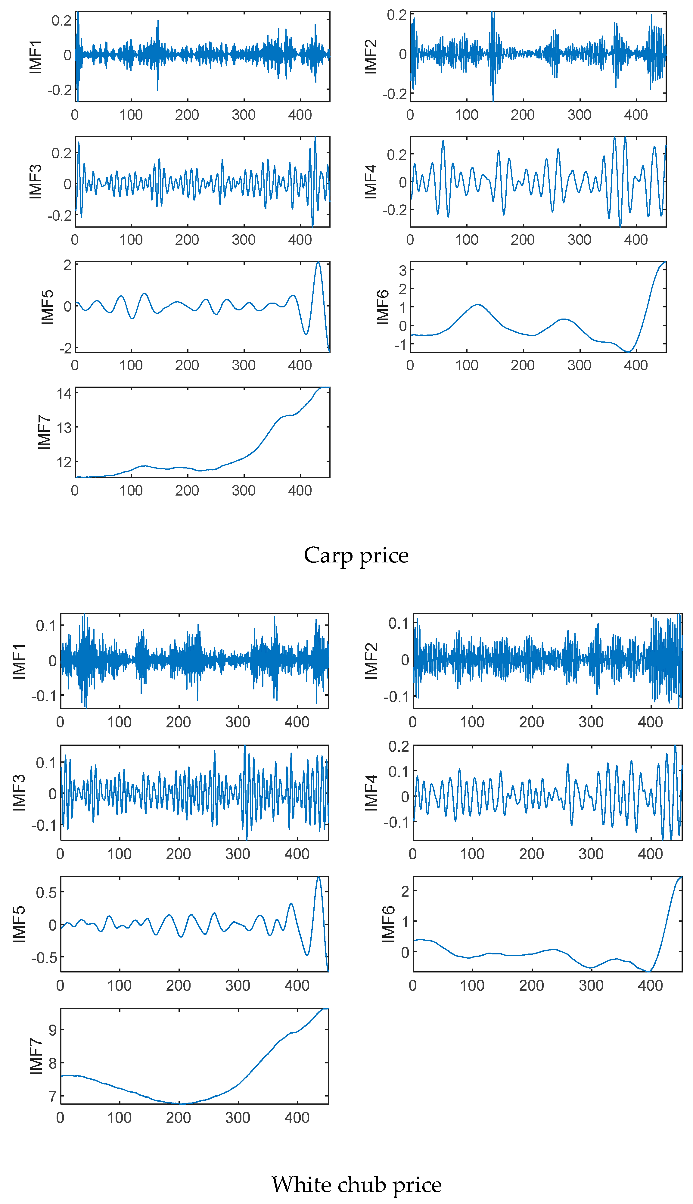
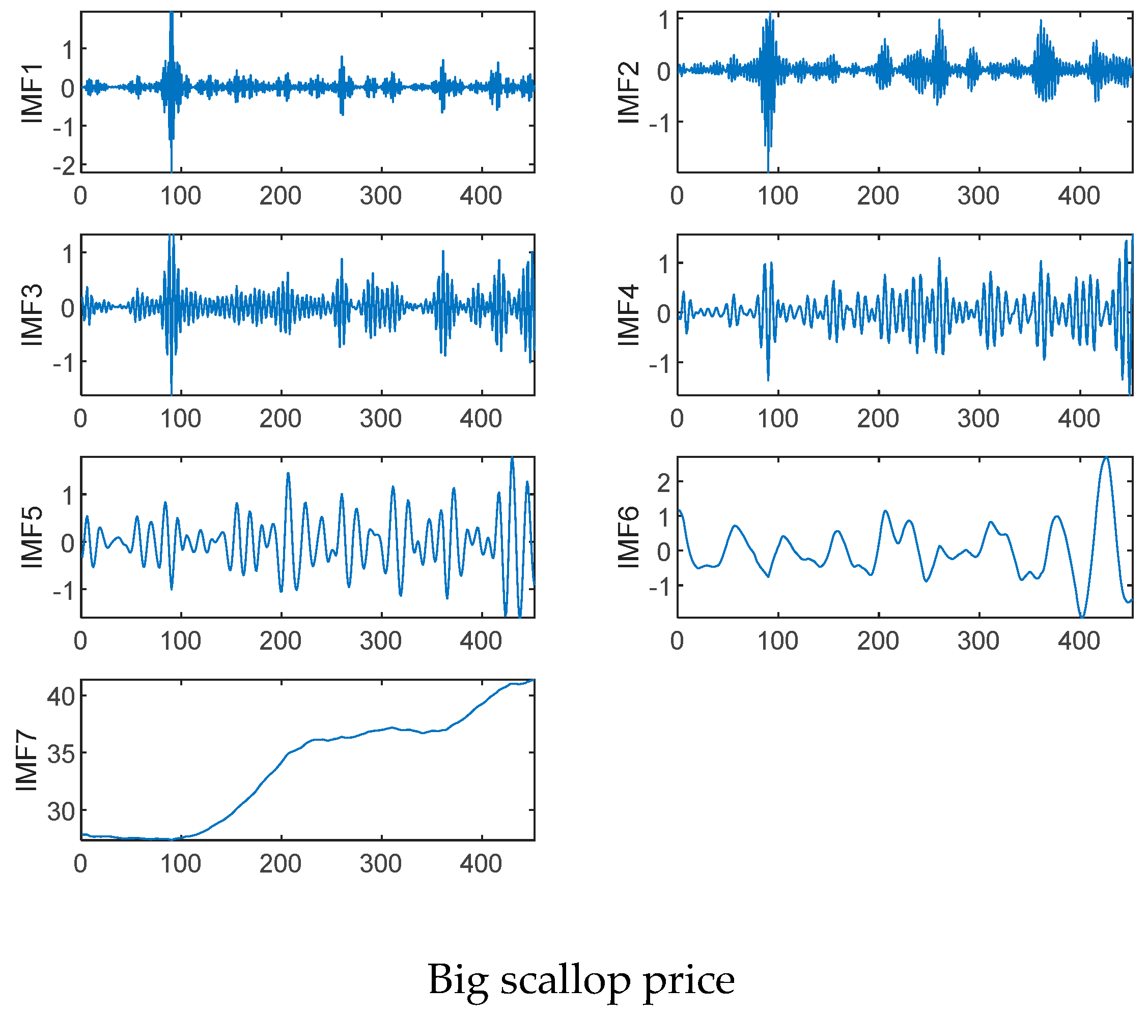
VMD parameters are set as follows: The VMD decomposition layers of grass carp and crucian carp price data set are seven layers. The VMD decomposition layer of carp, white chub and big scallop price data set is eight layers. The convergence tolerance . The empirical modal decomposition (EMD) results for each dataset are shown below (Figure 4 and Figure 5).
From the above figure we can see that the IMF components in the upper layers are strongly non-linear and unstable during the decomposition of EMD and VMD. Therefore, it is extremely crucial to predict the IMF components in the upper layers precisely. In addition, the EMD algorithm has the problem of modal mixing in the decomposition process, which greatly affects the subsequent prediction accuracy, while the application of the VMD algorithm can effectively tackle this problem.
4.3. Aquatic Product Price Forecasting Results Based on VMD-IBES-LSTM Model
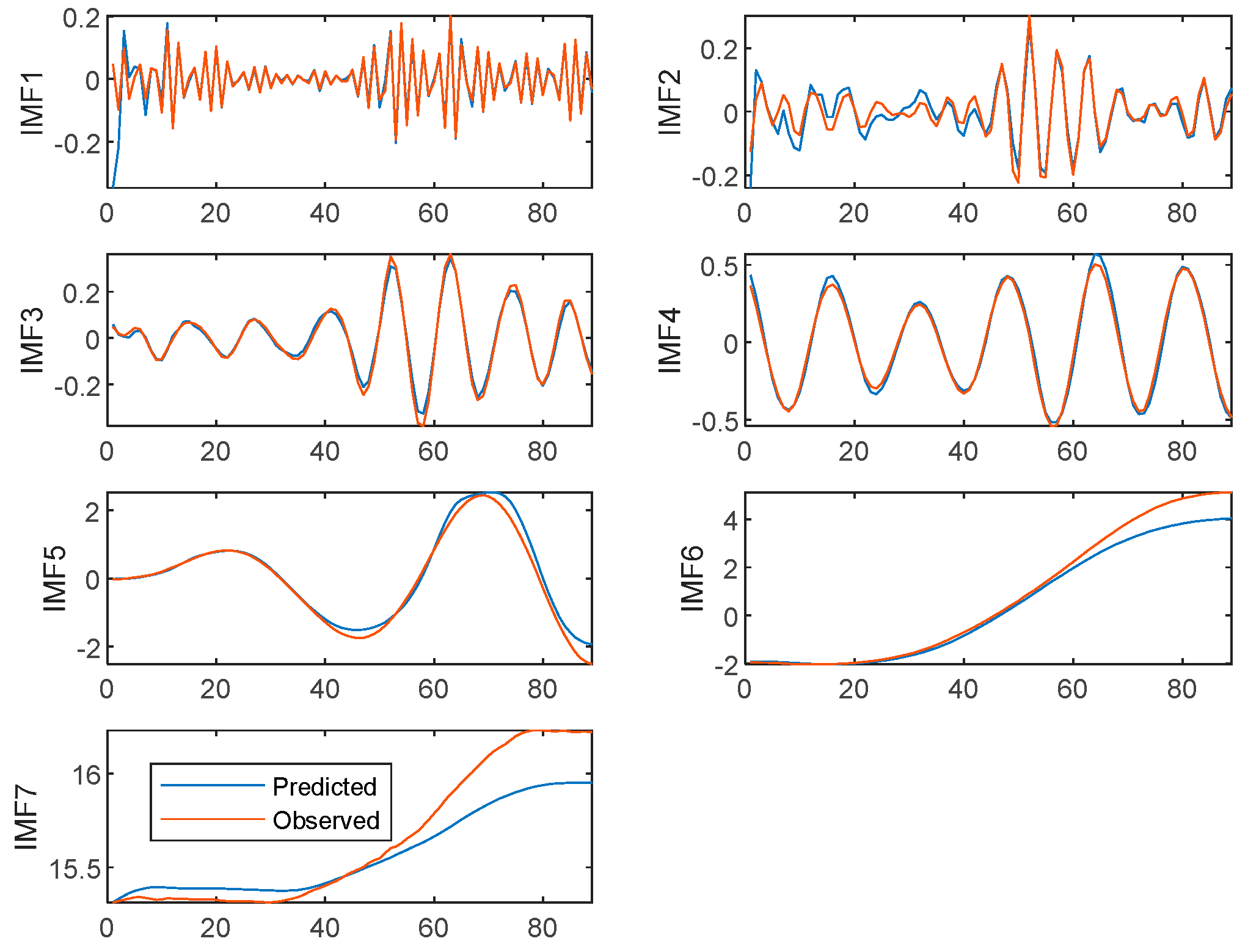
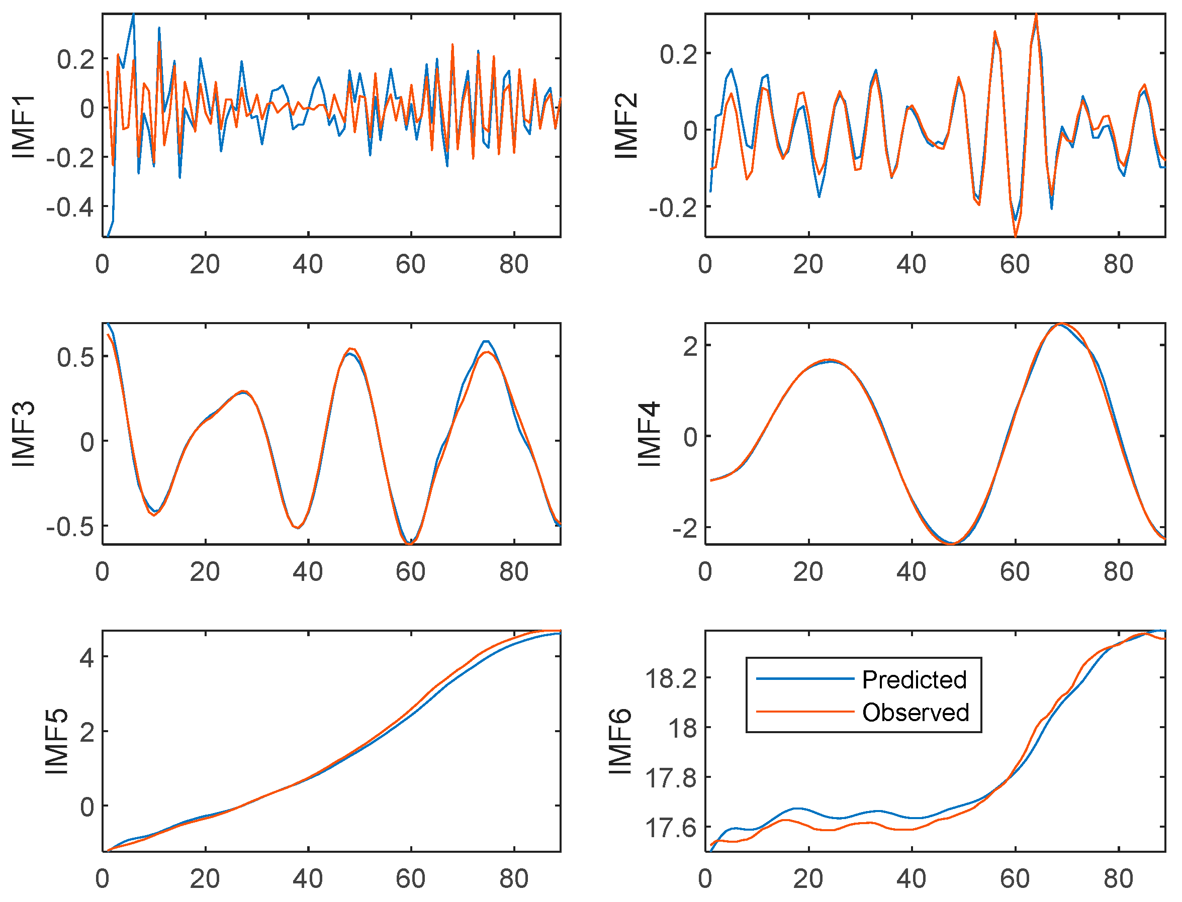
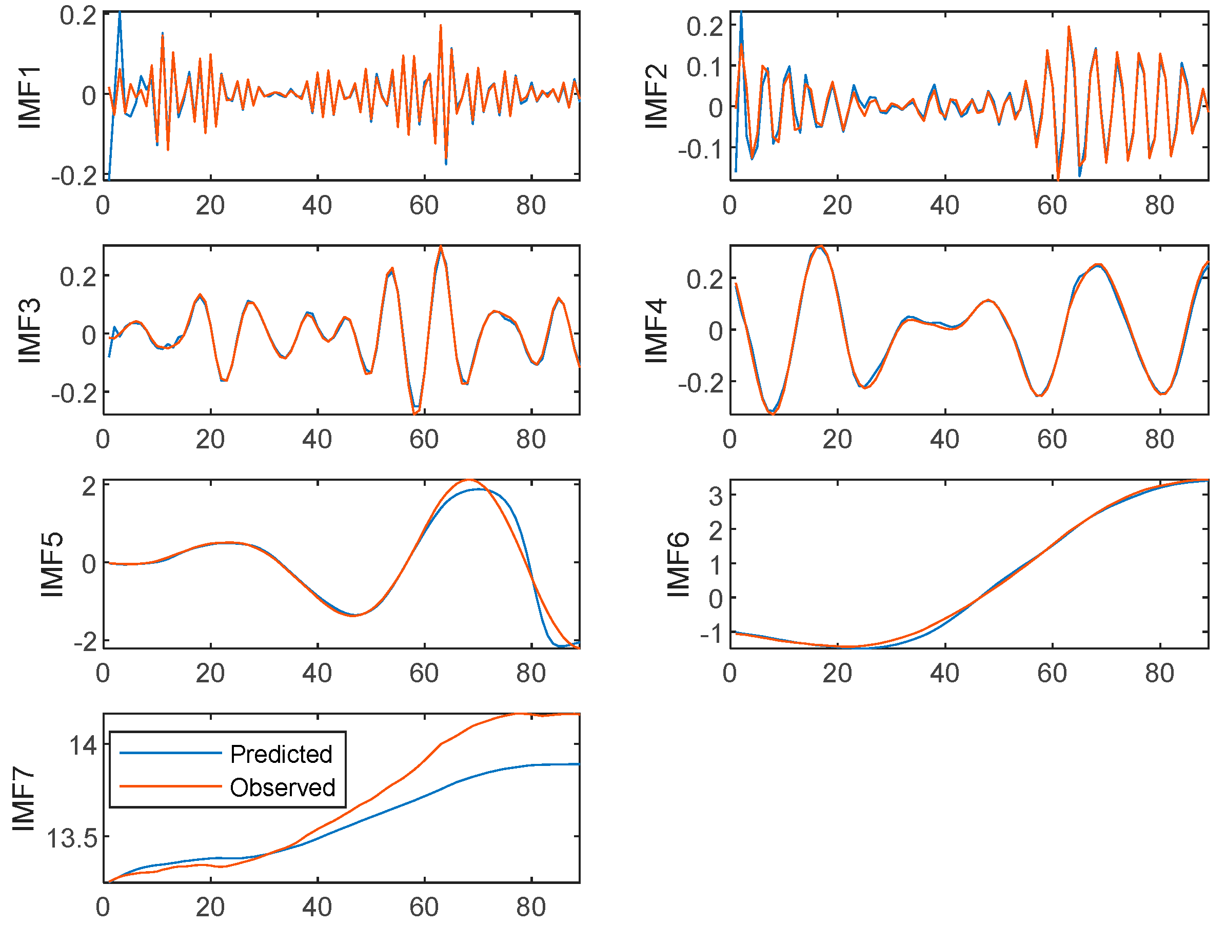
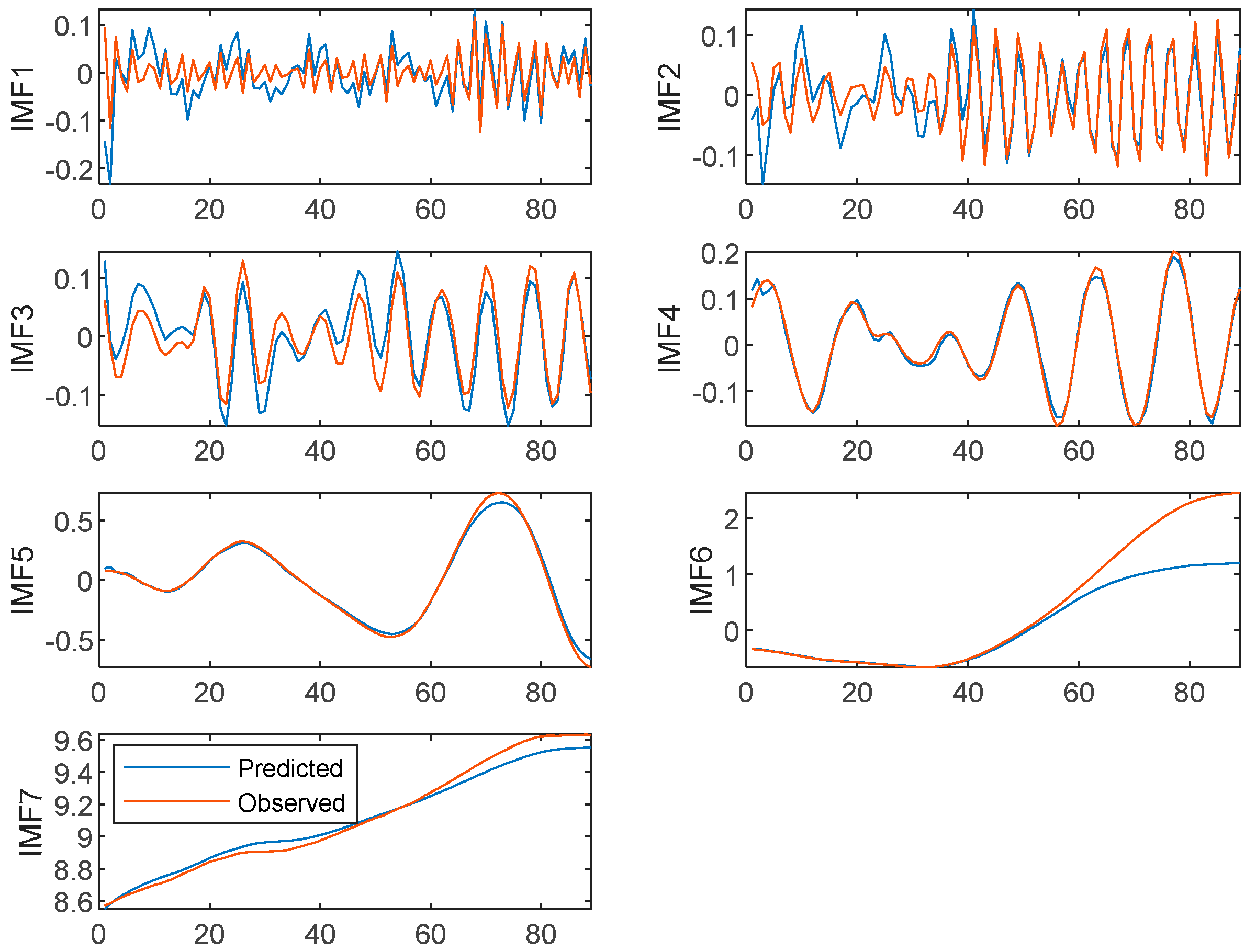
The parameter settings of the improved bald eagle search algorithm are as follows: the number of bald eagles is 5, the dim is 4, the range of learning rate is [0.001, 1], the number of neurons is [10, 500], and the maximum number of iterations is 100. Set the first 367 groups as the training set and the last 41 groups as the test set. The fitting results of each IMF price component are shown in the Figure 6, Figure 7, Figure 8, Figure 9 and Figure 10 below.
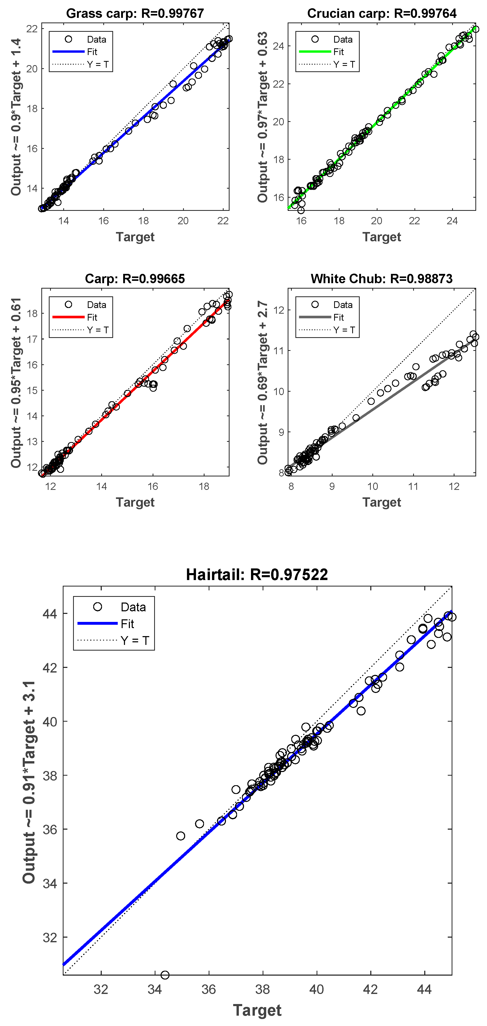
After summarizing each IMF, the regression images of each dataset are as follows (Figure 11):
It can be seen from the above figure that the goodness of fit of the VMD-IBES-LSTM model on Grass carp, crucian carp, carp, white chub, and big scallop price is 0.99767, 0.99764, 0.99665, 0.98873, and 0.97522, respectively, which indicated that the VMD-IBES-LSTM model fits best on the grass carp price dataset, while the fit is relatively average on the big scallop price dataset.
The error analysis of each IMF component is shown in the Table 3 below.
4.4. Comparative Results and Discussion
To test and validate the effectiveness and superiority of the model that is proposed in this study. In this research, we selected the EMD-VMD-LSTM model [8], VMD-LSTM model [11], CEEMD-CNN-LSTM [12] model, MOGWO-LSSVM model [42], and the model that was proposed in this paper for comparison
- LSTM: The learning rate is 0.3%, the number of iterations is 100, the number of cells in the hidden layer is 200, the solver is set to adam, the gradient threshold is set to 1, and the mini-batch size is 32.
- CNN-LSTM: the maximum number of iterations is 100 and the learning rate is 0.003.
- BiLSTM: the number of iterations is 100. The number of cells in the hidden layer is 200. The learning rate is 0.3%.
- MOGWO: We set the smoothness and accuracy of the model as the objective function. Set the size of the repository to 30, the maximum number of iterations to 100, and the number of grey wolves to 100. Set the grid expansion parameter to 0.1. Set the leader Selection Pressure Parameter to 4.
- The error analysis for each comparison model is shown in the Table 4 as below.
5. Discussion
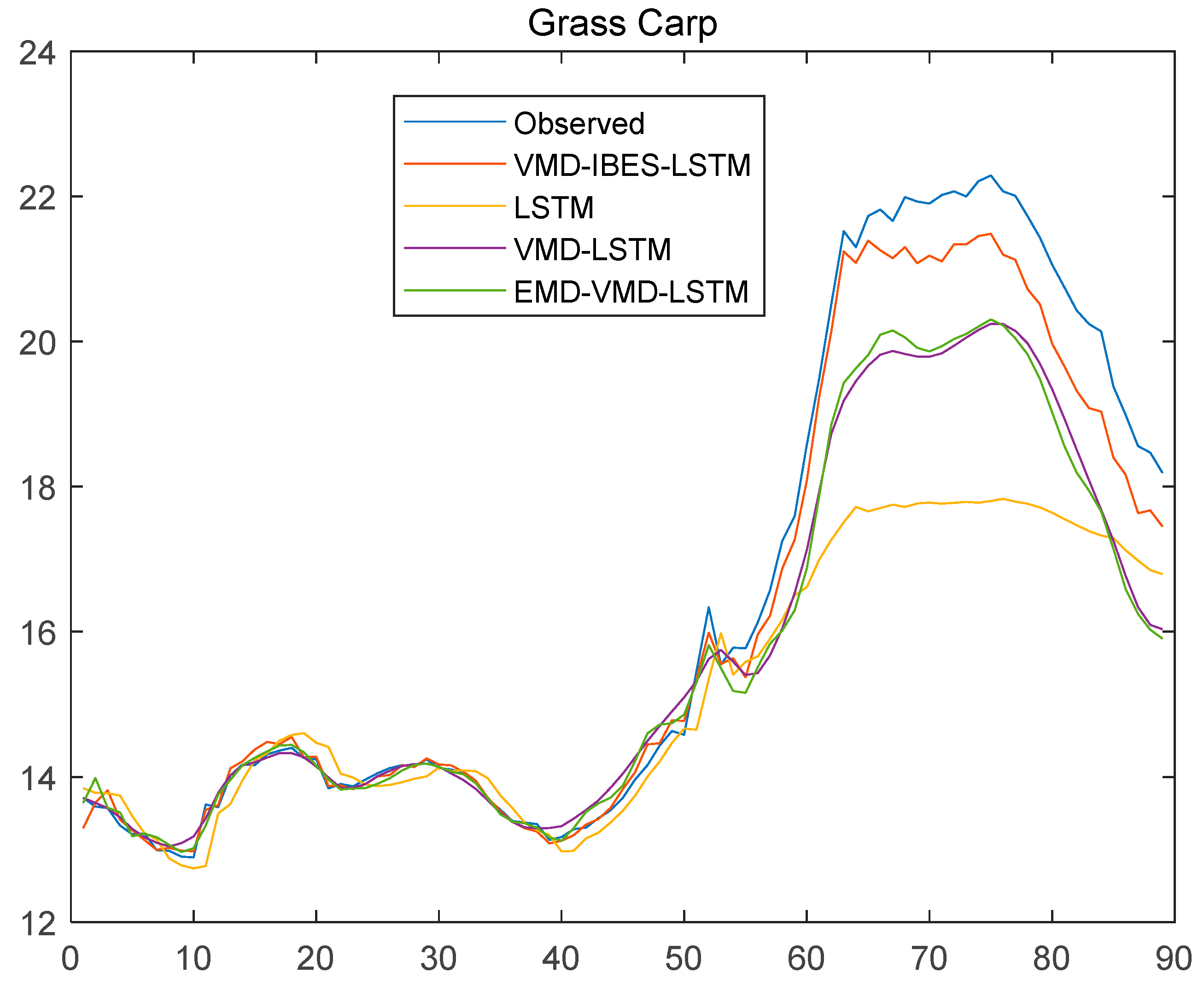
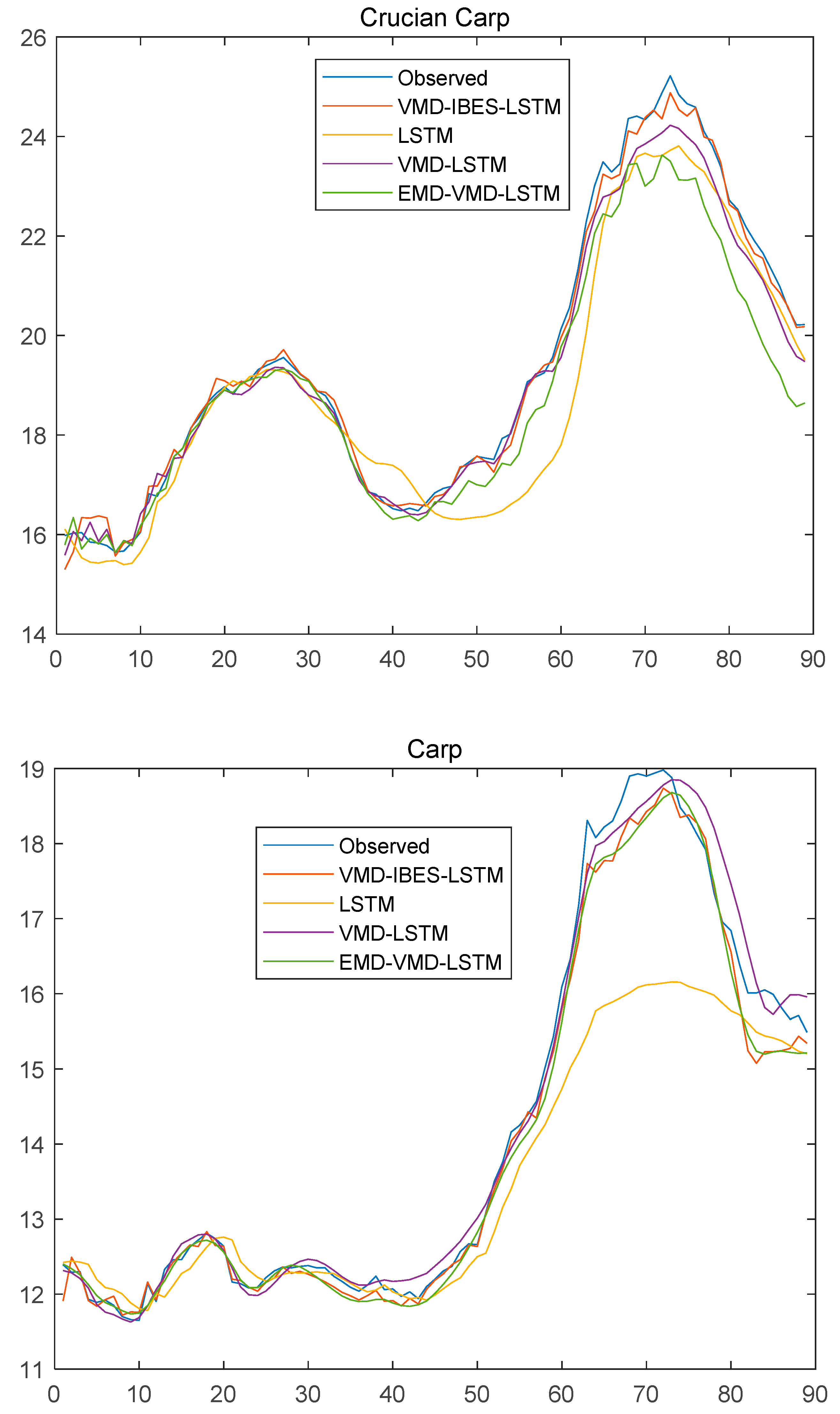
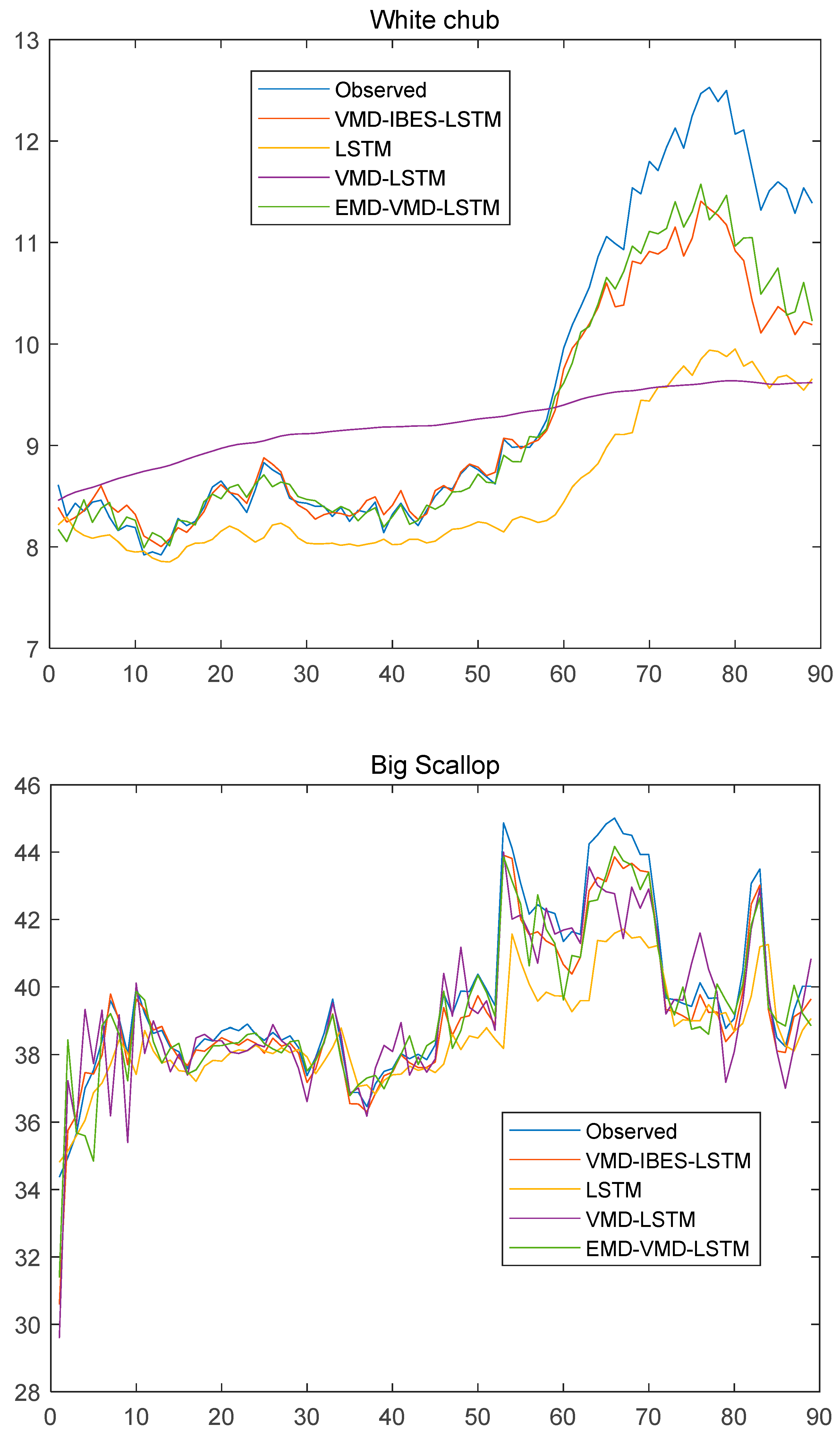
The fitting images of VMD-IBES-LSTM model and other models that were proposed in this study are as follows (Figure 12).
In the beginning, the models fit well because the fluctuations in grass carp, crucian carp, carp, and chub prices were small. However, with the passage of time, the fit of the single model (LSTM) becomes progressively worse, especially at the extremes. Taking the grass carp and carp price dataset as an example, it is clear that the prediction accuracy of the single model (LSTM) is poor at the extremes, which indicates the limitations of the single model in dealing with highly non-linear and non-stationary time series. Models that are based on the “decomposition-prediction-integration” idea such as the VMD-IBES-LSTM model, VMD-LSTM model, and EMD-VMD-LSTM model are less affected and have a better overall fit to the original dataset. To a higher degree, this indicated that compared to traditional single models (LSTM, BPNN, BiLSTM) and models that are based on the “feature extraction-prediction” idea (CNN-LSTM model, CNN-BiLSTM model), models that are based on the “decomposition-prediction-integration” models showed significant improvements in robustness and model accuracy.
In addition, from the above data results, it can be seen that the hybrid models that are based on the idea of “decomposition-prediction-integration” (e.g., VMD-LSTM) have better performance in terms of MSE, RMSE, and RMSE for each dataset. The MSE, RMSE, MAPE, and MAE of these hybrid models (e.g., NAR, LSTM, BPNN) are all smaller than those of the individual models (e.g., LSTM, BPNN), demonstrating that these hybrid models are significantly more accurate in prediction than the individual models. The reason for this analysis may lie in the fact that signal decomposition techniques can effectively solve problems such as prediction difficulties that are caused by the non-smoothness of time series data, significantly reducing the complexity of the data, and providing the possibility of improving the prediction accuracy of the models.
From the above figure, it can be seen that the VMD-IBES-LSTM model proposed in this study outperforms VMD-LSTM, CNN-BiLSTM, Bayes-BiLSTM and other models on each dataset. The improvement in the accuracy of the model is mainly in the following aspects.
- (1)
- The variational modal decomposition is used to decompose the fish price dataset into several IMF components, which can effectively reduce the non-linearity and non-smoothness of the dataset and improve the accuracy of the model.
- (2)
- An improved optimization algorithm is used to optimise each hyperparameter of the LSTM. In LSTM, the choice of parameters has an extremely important impact on the accuracy of the model. In previous studies, although scholars have proposed models that are based on the idea of “decomposition-prediction-integration” that can effectively improve the accuracy of prediction, less attention has been paid to the selection of parameters. The bald eagle search algorithm has received a lot of attention because of its advantages such as strong merit-seeking ability and difficulty in falling into local optimality. Thus, in this study, an improved bald eagle search algorithm was selected to optimize the hyperparameters of the LSTM.
- (3)
- A long short-term memory network was used to predict the individual IMF components. Compared with the traditional recurrent neural network, LSTM can effectively overcome the problem of gradient explosion and gradient disappearance with an increasing number of iterations of the traditional recurrent neural network. Thus, the VMD-IBES-LSTM model that was proposed in this study is effective and competitive.
Based on the above model and results, we would like to make the following policy recommendations.
- Data collection standards should be improved. The cross-fertilization of agricultural data and information technology should be strengthened and a unified system of data collection standards, including data collection and storage, should be established. A unified standard system should be formed through standardized data types, classifications, storage, interfaces, etc.
- Information analysis should be strengthened. First, we should actively study the analysis models, both to strengthen the study of the adaptability of existing models, such as time series, autoregressive models, moving average models, mixed autoregressive-moving average models, vector autoregressive models, etc., and to study new models that are based on existing data. Secondly, we should strengthen the cross analysis of different disciplines. Agricultural monitoring and early warning is a multidisciplinary field that requires both economic analysis and the integrated use of information technology, computer technology, database technology, and agricultural technology. Third, special analyses should be carried out in conjunction with different target groups. It is necessary to take full account of the economic operation of agriculture, taking into account reasonable fluctuations in the prices of agricultural products, as well as the returns of producers and the benefits to consumers. At the same time, technology is actively used to liberate manpower and increase labor productivity.
- The construction of the agricultural Internet of Things should be strengthened to improve the efficiency of agricultural products production. The agricultural Internet of Things is the application of Internet of Things technology in agricultural production, It is a specific application of agricultural production, management, and services, using various types of sensing devices to collect information about the agricultural production process, logistics of agricultural products, and animals and plants. It uses various sensing devices to collect information about the agricultural production process, the logistics of agricultural products, and the plants and animals themselves, and to transmit them through wireless sensor networks, mobile communication wireless networks, and the Internet. The information that was obtained is fused and processed through wireless sensor networks, mobile communication wireless networks, and internet transmission, and finally, through intelligent operation terminals, the process monitoring, scientific decision-making, and real-time services are realized for the pre-production, production, and post-production of agricultural products.
However, the method that was proposed in this study can be improved in the following aspects:
- (1)
- In this study, LSTM is used to predict fish prices. While there are many improved versions of LSTM, including Bi-LSTM, Adaptive Neuro-Fuzzy Inference System (ANFIS), etc., the above methods can be compared with the model that was proposed in this study.
- (2)
- The improved bald eagle search algorithm that was proposed in this study can also be combined with other optimisation algorithms (e.g., gravitational search algorithm, etc.) to subsequently optimize the parameters of the machine learning prediction model.
- (3)
- There are still some errors in the accuracy of the model that was proposed in this paper. The reasons for this are mainly the following. Price fluctuations of aquatic products are closely related to a variety of factors, such as the supply and demand of aquatic products, policy changes, consumer preferences, etc. In subsequent studies, consideration can be given to adding the above-mentioned influencing factors to further improve the accuracy of the model.
6. Conclusions
As an essential resource, the price trend of aquatic products has a crucial impact on economic and social development. To address the non-linear and non-stationary characteristics of aquatic product prices, this paper proposes a new hybrid VMD-IBES-LSTM model for fish price forecasting and compares with VMD-LSTM and other models. The results indicated that the VMD-IBES-LSTM model outperforms the other listed models in MSE, RMSE, MAE, and MAPE indicators. Ultimately, based on the above model, we put forward three policy recommendations.
However, the model that was proposed in this study can still be improved in the following aspects. (1) Consider other improved versions of the LSTM, such as Bi-LSTM and GRU, for comparison testing. (2) It can be combined with other optimization algorithms to verify whether the accuracy of the model has been improved. (3) The inclusion of factors that are closely related to aquatic product prices can be considered to further improve the prediction accuracy of the model. On 31 January 2020, the World Health Organization listed the epidemic situation of novel coronavirus as a public health event of international concern. Cities in China adopted the strategy of “closing cities” and isolation. The aquatic product trade fell into a stagnant state. Changes in the external factors in the short-term led to a decline in the prediction accuracy of this model. Some studies also show that the prediction accuracy of the SARIMA model decreases with time, which is more accurate when predicting the values of the next three to six periods, but when the prediction range exceeds six periods, the simulation effect becomes worse, and the prediction error gradually increases. The same conclusion has been reached in the actual prediction process in this paper. It can be seen from the comparison between the actual value and the predicted value in Table 4 that the relative error of prediction gradually increases with the passage of time. The short-term changes of the internal and external factors also need to re-evaluate their parameters regularly according to the constantly updated data, so as to improve the accuracy of model prediction.
Author Contributions
J.W.: Writing—original draft, investigation, visualization, writing—review & editing. Z.Y.: Methodology, supervision, validation. Y.H.: Writing—original draft, diagram and flowchart preparation, writing-review & editing. D.W.: Conceptualization, formal analysis, resources. Z.Y.: Investigation, visualization. All authors have read and agreed to the published version of the manuscript.
Funding
This research was funded by the China Education Ministry of Humanities and Social Science Research Youth Fund project (No. 18YJCZH192). Ministry of Finance and Ministry of agriculture and rural areas: national special fund for the construction of modern agricultural industrial technology system “Industrial Economic Research on national marine fish industrial technology system” (No. CARS-47-G29). Major project of National Social Science Fund “Research on the development strategy of China’s deep blue fishery under the background of accelerating the construction of a marine power” (No. 21 & ZD100).
Institutional Review Board Statement
Not applicable.
Informed Consent Statement
Not applicable.
Data Availability Statement
All experimental data in this paper come from Price information system of national agricultural products wholesale market in China: http://pfsc.agri.cn/#/indexPage (accessed on 4 April 2022).
Acknowledgments
Thanks to the computing science center of Shanghai Ocean University for its support for scientific research.
Conflicts of Interest
The authors declare no conflict of interest.
References
- Fabinyi, M.; Liu, N. The social context of the chinese food system: An ethnographic study of the beijing seafood market. Sustainability 2016, 8, 244. [Google Scholar] [CrossRef]
- Sun, Y.; Lian, F.; Guo, W.Y.; Yang, Z.Z. The spatial evolution and optimization of supply channels for marine products consumed in China. Marit. Policy Manag. 2022, 8, 1–23. [Google Scholar] [CrossRef]
- Fabinyi, M. Historical, cultural and social perspectives on luxury seafood consumption in China. Environ. Conserv. 2012, 39, 83–92. [Google Scholar] [CrossRef]
- Miao, M.; Liu, H.; Chen, J. Factors affecting fluctuations in China’s aquatic product exports to Japan, the USA, South Korea, Southeast Asia, and the EU. Aquacult. Int. 2021, 29, 2507–2533. [Google Scholar] [CrossRef]
- Wang, R.; Li, C.; Fu, W.; Tang, G. Deep learning method based on gated recurrent unit and variational mode decomposition for short-term wind power interval prediction. IEEE Trans. Neural Netw. Learn. Syst. 2019, 31, 3814–3827. [Google Scholar] [CrossRef]
- Huang, Y.; Dai, X.; Wang, Q.; Zhou, D. A hybrid model for carbon price forecasting using GARCH and long short-term memory network. Appl. Energy 2021, 285, 116485. [Google Scholar] [CrossRef]
- Lin, Y.; Lu, Q.; Tan, B.; Yu, Y. Forecasting energy prices using a novel hybrid model with variational mode decomposition. Energy 2022, 246, 123366. [Google Scholar] [CrossRef]
- Sun, W.; Huang, C. A novel carbon price prediction model combines the secondary decomposition algorithm and the long short-term memory network. Energy 2020, 207, 118294. [Google Scholar] [CrossRef]
- Liang, Y.; Lin, Y.; Lu, Q. Forecasting gold price using a novel hybrid model with ICEEMDAN and LSTM-CNN-CBAM. Expert Syst. Appl. 2022, 206, 117847. [Google Scholar] [CrossRef]
- Huang, Y.; Deng, Y. A new crude oil price forecasting model based on variational mode decomposition. Knowl.-Based Syst. 2021, 213, 106669. [Google Scholar] [CrossRef]
- Liu, Y.; Yang, C.; Huang, K.; Gui, W. Non-ferrous metals price forecasting based on variational mode decomposition and LSTM network. Knowl.-Based Syst. 2020, 188, 105006. [Google Scholar] [CrossRef]
- Rezaei, H.; Faaljou, H.; Mansourfar, G. Stock price prediction using deep learning and frequency decomposition. Expert Syst. Appl. 2021, 169, 114332. [Google Scholar] [CrossRef]
- Duran, N.M.; Maciel, E.D.S.; Galvao, J.A.; Savay-da-Silva, L.K.; Sonati, J.G.; Oetterer, M. Availability and consumption of fish as convenience food—Correlation between market value and nutritional parameters. Food Sci. Technol.-Brazil 2018, 37, 65–69. [Google Scholar] [CrossRef]
- Nam, J.; Sim, S. Forecast accuracy of abalone producer prices by shell size in the republic of korea: Modified diebold–mariano tests of selected autoregressive models. Aquacult. Econ. Manag. 2017, 22, 474–489. [Google Scholar] [CrossRef]
- Mazliana, M.; Raja, R.P.; Ho, M.K. Forecasting Prices of Fish and Vegetable using Web Scraped Price Micro Data. Int. J. Rec. Eng. 2019, 7, 251–256. [Google Scholar]
- Hasan, M.R.; Dey, M.M.; Engle, C.R. Forecasting monthly catfish (ictalurus punctatus.) pond bank and feed prices. Aquacult. Econ. Manag. 2019, 23, 86–110. [Google Scholar] [CrossRef]
- Gordon, D.V. A short-run ARDL-bounds model for forecasting and simulating the price of lobster. Mar. Resour. Econ. 2020, 35, 43–63. [Google Scholar] [CrossRef]
- Guillen, J.; Maynou, F. Characterisation of fish species based on ex-vessel prices and its management implications: An application to the spanish mediterranean. Fish. Res. 2015, 167, 22–29. [Google Scholar] [CrossRef]
- Nguyen, H.T.K.; Thu, T.T.N.; Lebailly, P.; Azadi, H. Economic challenges of the export-oriented aquaculture sector in Vietnam. J. Appl. Aquac. 2019, 31, 367–383. [Google Scholar] [CrossRef]
- Li, H.; Gao, X.; Cheng, K. The application of wavelet neural network in prediction of the fish price. Appl. Mech. Mater. 2014, 687, 1945–1949. [Google Scholar] [CrossRef]
- Duan, Q.; Zhang, L.; Wei, F.; Xiao, X.; Wang, L. Forecasting model and validation for aquatic product price based on time series GA-SVR. Trans. Chin. Soc. Agric. Eng. 2017, 33, 308–314. [Google Scholar]
- Bloznelis, D. Short term salmon price forecasting. J. Forecast. 2018, 37, 151–169. [Google Scholar] [CrossRef]
- Yuan, H.; Chen, Y.; Ju, J. A CBR Based Prediction Method for Web Aquatic Products Prices. Int. J. Comput. Int. Sys. 2007, 195–200. [Google Scholar]
- Shi, J.; Leau, Y.B.; Li, K.; Park, Y.J.; Yan, Z. Optimization and Decomposition Methods in Network Traffic Prediction Model: A Review and Discussion. IEEE Access 2020, 8, 202858–202871. [Google Scholar] [CrossRef]
- Dragomiretskiy, K.; Zosso, D. Variational mode decomposition. IEEE Trans. Signal Process. 2013, 62, 531–544. [Google Scholar] [CrossRef]
- Alsattar, H.A.; Zaidan, A.A.; Zaidan, B.B. Novel meta-heuristic bald eagle search optimisation algorithm. Artif. Intell. Rev. 2020, 53, 2237–2264. [Google Scholar] [CrossRef]
- Angayarkanni, S.A.; Sivakumar, R.; Ramana Rao, Y.V. Hybrid Grey Wolf: Bald Eagle search optimized support vector regression for traffic flow forecasting. J. Amb. Intel. Hum. Comp. 2021, 12, 1293–1304. [Google Scholar] [CrossRef]
- Li, L.L.; Liu, Z.F.; Tseng, M.L.; Zheng, S.J.; Lim, M.K. Improved tunicate swarm algorithm: Solving the dynamic economic emission dispatch problems. Appl. Soft Comput. 2021, 108, 107504. [Google Scholar] [CrossRef]
- Chen, S.; Wang, S. An Optimization Method for an Integrated Energy System Scheduling Process Based on NSGA-II Improved by Tent Mapping Chaotic Algorithms. Processes 2020, 8, 426. [Google Scholar] [CrossRef]
- Hochreiter, S.; Schmidhuber, J. Long short-term memory. Neural Comput. 1997, 9, 1735–1780. [Google Scholar] [CrossRef]
- Zhang, J.; Zhu, Y.; Zhang, X.; Ye, M.; Yang, J. Developing a long short-term memory (LSTM) based model for predicting water table depth in agricultural areas. J. Hydrol. 2018, 561, 918–929. [Google Scholar] [CrossRef]
- Wang, X.; Wang, Y.; Yuan, P.; Wang, L.; Cheng, D. An adaptive daily runoff forecast model using VMD-LSTM-PSO hybrid approach. Hydrol. Sci. J. 2021, 66, 1488–1502. [Google Scholar] [CrossRef]
- Fang, Z.; Wang, Y.; Peng, L.; Hong, H. Predicting flood susceptibility using LSTM neural networks. J. Hydrol. 2021, 594, 125734. [Google Scholar] [CrossRef]
- Chen, Y.; Lin, M.; Yu, R.; Wang, T. Research on simulation and state prediction of nuclear power system based on LSTM neural network. Sci. Technol. Nucl. Install. 2021, 2021, 8839867. [Google Scholar] [CrossRef]
- Fukuoka, R.; Suzuki, H.; Kitajima, T.; Kuwahara, A.; Yasuno, T. Wind Speed Prediction Model Using LSTM and 1D-CNN. J. Signal Process. 2018, 22, 207–210. [Google Scholar] [CrossRef]
- Ehsan, M.A.; Shahirinia, A.; Zhang, N.; Oladunni, T. Wind Speed Prediction and Visualization Using Long Short-Term Memory Networks (LSTM). In Proceedings of the 10th International Conference on Information Science and Technology (ICIST), Bath, London, and Plymouth, UK, 9–15 September 2020; pp. 234–240. [Google Scholar]
- Troiano, L.; Villa, E.M.; Loia, V. Replicating a Trading Strategy by Means of LSTM for Financial Industry Applications. IEEE Trans. Ind. Inform. 2018, 14, 3226–3234. [Google Scholar] [CrossRef]
- Sundermeyer, M.; Schlüter, R.; Ney, H. LSTM Neural Networks for Language Modeling. In Proceedings of the Thirteenth Annual Conference of the International Speech Communication Association, Portland, OR, USA, 9–13 September 2012. [Google Scholar]
- Wu, S.; Feng, F.; Zhu, J.; Wu, C.; Zhang, G. A method for determining intrinsic mode function number in variational mode decomposition and its application to bearing vibration signal processing. Shock. Vib. 2020, 2020, 8304903. [Google Scholar] [CrossRef]
- Li, Y.; Li, Y.; Chen, X.; Yu, J. Research on ship-radiated noise denoising using secondary variational mode decomposition and correlation coefficient. Sensors 2017, 18, 48. [Google Scholar] [CrossRef]
- Zhang, K.; Cao, H.; Thé, J.; Yu, H. A hybrid model for multi-step coal price forecasting using decomposition technique and deep learning algorithms. Appl. Energy 2022, 306, 118011. [Google Scholar] [CrossRef]
- Bai, L.; Liu, Z.; Wang, J. Novel hybrid extreme learning machine and multi-objective optimization algorithm for air pollution prediction. Appl. Math. Model. 2022, 106, 177–198. [Google Scholar] [CrossRef]
Figure 1.
Structure of LSTM.

Figure 2.
Flow chart of VMD-IBES-LSTM model.

Figure 3.
Dataset images.

Figure 4.
The outcome of EMD for each aquatic product price dataset. The variational modal decomposition (VMD) results for each dataset are shown below.
Figure 4.
The outcome of EMD for each aquatic product price dataset. The variational modal decomposition (VMD) results for each dataset are shown below.


Figure 5.
The outcome of VMD for each aquatic product price dataset.


Figure 6.
Fitting results of IMF components in grass carp price dataset.

Figure 7.
Fitting results of IMF components of crucian carp price dataset.

Figure 8.
Results of fitting each IMF component to the carp price dataset.

Figure 9.
Fitting results for each IMF component of the white chub price dataset.

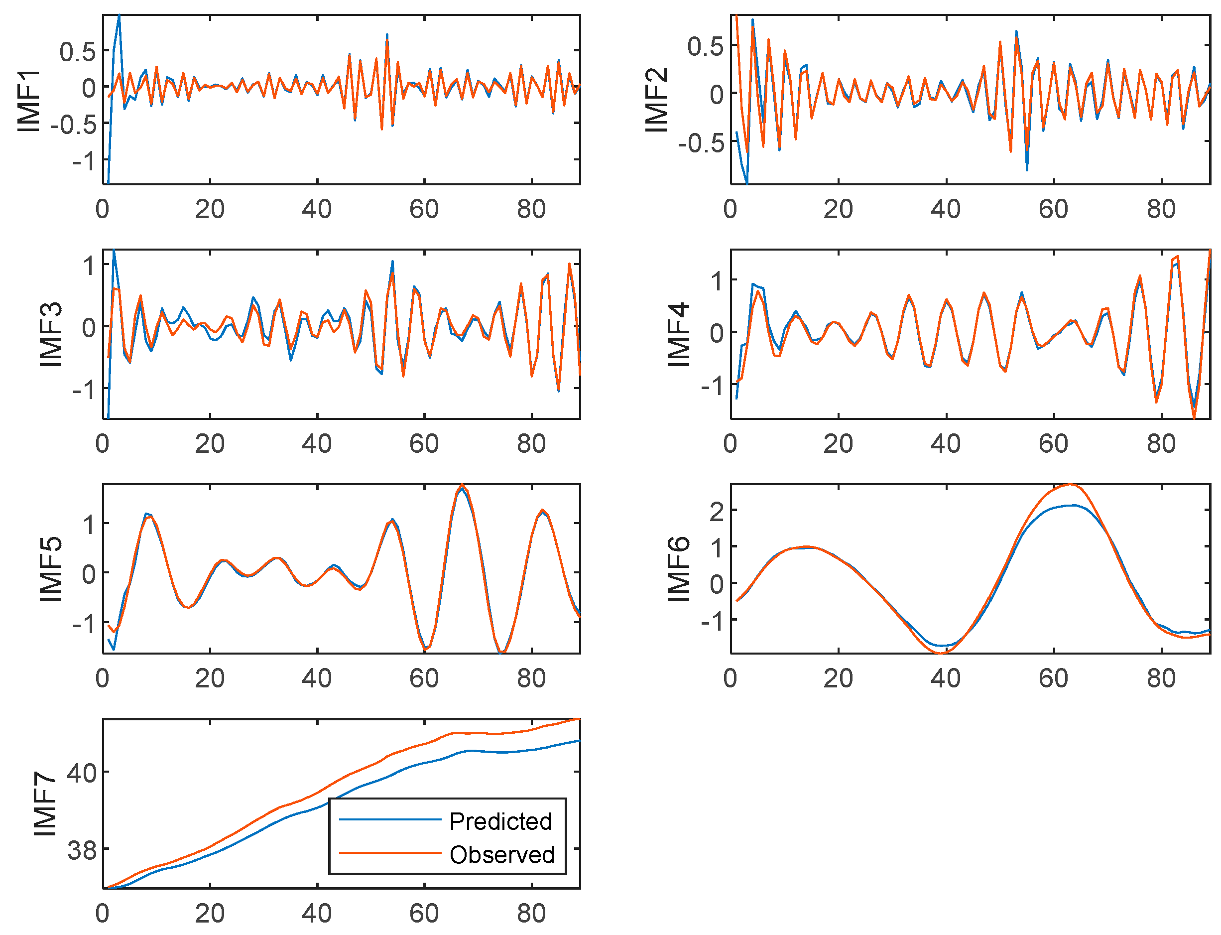
Figure 10.
Fitting results for each IMF component of the big scallop price dataset.

Figure 11.
Data regression image of each aquatic product price test set.

Figure 12.
Fitting images of each model.


Table 1.
Descriptive statistics of the data set.
| Minimum Value | Maximum Value | Mean | Standard Deviation | |
|---|---|---|---|---|
| Grass carp | 11.73 | 22.29 | 14.2 | 2.08 |
| Crucian carp | 12.99 | 25.22 | 16.1 | 2.34 |
| Carp | 10.64 | 18.98 | 12.25 | 1.57 |
| White Chub | 6.43 | 12.53 | 7.63 | 1.23 |
| Big Scallop | 18.04 | 45.01 | 33.7 | 4.9 |
Table 2.
Correlation coefficients for datasets.
| Grass Carp | Crucian CARP | Carp | White Chub | Big Scallop | |
|---|---|---|---|---|---|
| Grass Carp | 1 | 0.83 | 0.78 | 0.81 | 0.43 |
| Crucian carp | 1 | 0.73 | 0.78 | 0.56 | |
| Carp | 1 | 0.79 | 0.47 | ||
| White Chub | 1 | 0.45 | |||
| Big Scallop | 1 |
Table 3.
Error analysis table.
| MSE | RMSE | MAE | MAPE | ||
|---|---|---|---|---|---|
| Grass Carp | IMF1 | 0.0020 | 0.0447 | 0.0150 | 0.3840 |
| IMF2 | 0.0010 | 0.0316 | 0.0240 | 1.2040 | |
| IMF3 | 0.0003 | 0.0173 | 0.0140 | 0.2390 | |
| IMF4 | 0.0001 | 0.0100 | 0.0273 | 0.3378 | |
| IMF5 | 0.0440 | 0.2098 | 0.1401 | 0.2438 | |
| IMF6 | 0.2473 | 0.4973 | 0.3250 | 0.1741 | |
| IMF7 | 0.0235 | 0.1532 | 0.1136 | 0.0071 | |
| Crucian carp | IMF1 | 0.0130 | 0.1140 | 0.0731 | 6.2650 |
| IMF2 | 0.0011 | 0.03317 | 0.0250 | 1.112 | |
| IMF3 | 0.0009 | 0.0300 | 0.0213 | 0.4643 | |
| IMF4 | 0.0049 | 0.0700 | 0.0499 | 0.1003 | |
| IMF5 | 0.0138 | 0.1175 | 0.0948 | 0.0842 | |
| IMF6 | 0.0014 | 0.0374 | 0.0330 | 0.0019 | |
| Carp | IMF1 | 0.0010 | 0.0316 | 0.0121 | 0.5859 |
| IMF2 | 0.0007 | 0.0265 | 0.0146 | 1.1712 | |
| IMF3 | 0.0001 | 0.0100 | 0.0074 | 0.5499 | |
| IMF4 | 0.0002 | 0.0140 | 0.0100 | 0.3814 | |
| IMF5 | 0.0333 | 0.1824 | 0.1044 | 0.2633 | |
| IMF6 | 0.0058 | 0.07622 | 0.0589 | 0.0724 | |
| IMF7 | 0.0269 | 0.1640 | 0.1227 | 0.0088 | |
| White chub | IMF1 | 0.0017 | 0.0412 | 0.0297 | 3.2284 |
| IMF2 | 0.0009 | 0.0300 | 0.0239 | 0.9942 | |
| IMF3 | 0.0010 | 0.0316 | 0.0285 | 1.0449 | |
| IMF4 | 0.0001 | 0.0100 | 0.0085 | 0.1973 | |
| IMF5 | 0.0009 | 0.0300 | 0.0212 | 0.3164 | |
| IMF6 | 0.2717 | 0.5212 | 0.2926 | 1.9635 | |
| IMF7 | 0.0026 | 0.0510 | 0.0427 | 0.0046 | |
| Hairtail | IMF1 | 0.0293 | 0.1712 | 0.0590 | 0.9651 |
| IMF2 | 0.0254 | 0.1594 | 0.0629 | 0.4858 | |
| IMF3 | 0.0267 | 0.1634 | 0.1055 | 1.8694 | |
| IMF4 | 0.0150 | 0.1225 | 0.0741 | 0.6865 | |
| IMF5 | 0.0060 | 0.0775 | 0.0513 | 0.2352 | |
| IMF6 | 0.0378 | 0.1944 | 0.1277 | 0.3146 | |
| IMF7 | 0.1669 | 0.4085 | 0.3791 | 0.0095 |
Table 4.
Comparison of various models in prediction performance.
| VMD-IBES-LSTM | LSTM | BPNN | CNN-LSTM | BiLSTM | CNN-BiLSTM | Bayes-BiLSTM | VMD-LSTM | EMD-VMD-LSTM | MOGWO-LSSVM | CEEMD-CNN-LSTM | ||
|---|---|---|---|---|---|---|---|---|---|---|---|---|
| Grass carp | MSE | 0.230 | 4.260 | 5.700 | 7.540 | 20.970 | 8.539 | 3.507 | 1.430 | 1.460 | 1.358 | 6.281 |
| RMSE | 0.480 | 2.064 | 2.390 | 2.750 | 4.570 | 2.922 | 1.873 | 1.196 | 1.208 | 1.165 | 2.506 | |
| MAE | 0.016 | 0.065 | 5.040 | 0.080 | 0.180 | 0.088 | 0.058 | 0.041 | 0.040 | 0.037 | 0.110 | |
| MAPE | 0.320 | 1.310 | 1.690 | 1.690 | 3.340 | 1.804 | 1.168 | 0.801 | 0.804 | 0.739 | 1.993 | |
| Crucian carp | MSE | 0.046 | 0.880 | 2.750 | 5.860 | 10.670 | 5.717 | 0.142 | 0.160 | 0.710 | 1.716 | 2.921 |
| RMSE | 0.214 | 0.940 | 1.660 | 2.420 | 3.270 | 2.391 | 0.377 | 0.400 | 0.843 | 1.310 | 1.709 | |
| MAE | 0.008 | 0.036 | 1.460 | 0.070 | 0.160 | 0.071 | 0.014 | 0.015 | 0.028 | 0.049 | 0.053 | |
| MAPE | 0.157 | 0.720 | 1.330 | 1.570 | 3.070 | 1.582 | 0.276 | 0.304 | 0.600 | 1.013 | 1.157 | |
| Carp | MSE | 0.083 | 1.320 | 5.040 | 4.390 | 9.540 | 3.714 | 3.577 | 0.086 | 0.709 | 1.343 | 4.889 |
| RMSE | 0.288 | 1.150 | 2.240 | 2.100 | 3.100 | 1.927 | 1.891 | 0.293 | 0.842 | 1.159 | 2.211 | |
| MAE | 0.012 | 0.044 | 3.900 | 0.080 | 0.120 | 0.068 | 0.118 | 0.013 | 0.028 | 0.041 | 0.112 | |
| MAPE | 0.190 | 0.730 | 1.500 | 1.290 | 2.000 | 1.168 | 1.296 | 0.200 | 0.596 | 0.700 | 1.751 | |
| White chub | MSE | 0.240 | 1.630 | 6.020 | 3.600 | 6.360 | 3.577 | 0.282 | 0.253 | 0.242 | 1.589 | 2.403 |
| RMSE | 0.489 | 1.280 | 2.450 | 1.900 | 2.520 | 1.891 | 0.531 | 0.503 | 0.492 | 1.261 | 1.550 | |
| MAE | 0.032 | 0.091 | 1.200 | 0.120 | 0.230 | 0.118 | 0.034 | 0.033 | 0.039 | 0.082 | 0.118 | |
| MAPE | 0.350 | 0.960 | 2.160 | 1.300 | 2.310 | 1.296 | 0.365 | 0.362 | 0.318 | 0.887 | 1.227 | |
| Big Scallop | MSE | 0.470 | 2.820 | 4.540 | 7.420 | 142.700 | 7.107 | 6.520 | 1.326 | 0.814 | 3.665 | 5.108 |
| RMSE | 0.680 | 1.680 | 2.130 | 2.720 | 11.950 | 2.666 | 2.55 | 1.152 | 0.902 | 1.914 | 2.260 | |
| MAE | 0.012 | 0.030 | 1.690 | 0.050 | 0.260 | 0.049 | 0.042 | 0.020 | 0.016 | 0.035 | 0.049 | |
| MAPE | 0.490 | 2.220 | 1.630 | 2.100 | 10.670 | 2.016 | 1.740 | 0.794 | 0.65 | 1.426 | 1.972 |
Publisher’s Note: MDPI stays neutral with regard to jurisdictional claims in published maps and institutional affiliations. |
© 2022 by the authors. Licensee MDPI, Basel, Switzerland. This article is an open access article distributed under the terms and conditions of the Creative Commons Attribution (CC BY) license (https://creativecommons.org/licenses/by/4.0/).
Share and Cite
MDPI and ACS Style
Wu, J.; Hu, Y.; Wu, D.; Yang, Z. An Aquatic Product Price Forecast Model Using VMD-IBES-LSTM Hybrid Approach. Agriculture 2022, 12, 1185. https://doi.org/10.3390/agriculture12081185
AMA Style
Wu J, Hu Y, Wu D, Yang Z. An Aquatic Product Price Forecast Model Using VMD-IBES-LSTM Hybrid Approach. Agriculture. 2022; 12(8):1185. https://doi.org/10.3390/agriculture12081185
Chicago/Turabian StyleWu, Junhao, Yuan Hu, Daqing Wu, and Zhengyong Yang. 2022. "An Aquatic Product Price Forecast Model Using VMD-IBES-LSTM Hybrid Approach" Agriculture 12, no. 8: 1185. https://doi.org/10.3390/agriculture12081185
Note that from the first issue of 2016, this journal uses article numbers instead of page numbers. See further details here.