Hyperspectral-Based Classification of Managed Permanent Grassland with Multilayer Perceptrons: Influence of Spectral Band Count and Spectral Regions on Model Performance

Abstract

Detailed knowledge of botanical composition is a key factor for the sustainable and site-specific management of permanent grassland and facilitates an improvement in the performance and efficiency of livestock feeding. Spectral-based data acquisition combined with machine learning has the potential to classify species groups and plant parts in permanent grassland with high accuracy. However, a disadvantage of this method is the fact that hyperspectral sensors with a wide spectral range and fine spectral and high spatial resolution are costly and create large amounts of data. Therefore, the question arises as to whether these parameters are necessary for accurate grassland classification. Thus, the use of sensors with lower spectral and spatial resolution and correspondingly lower data processing requirements could be a conceivable approach. Therefore, we investigated the classification performance with reduced predictor sets formed by different approaches in permanent grassland. For pixel-based classification, a cross-validated mean accuracy of $86.1$% was reached using a multilayer perceptron (MLP) including all 191 available predictors, i.e., spectral bands. Using only 48 high-performing predictors, an accuracy of 80% could still be achieved. In particular, the spectral regions of 954 $\mathrm{n}$$\mathrm{m}$ to 956 $\mathrm{n}$$\mathrm{m}$, 684 $\mathrm{n}$$\mathrm{m}$ to 744 $\mathrm{n}$$\mathrm{m}$ and 442 $\mathrm{n}$$\mathrm{m}$ to 444 $\mathrm{n}$$\mathrm{m}$ contributed most to the classification performance. These results provide a promising basis for future data acquisition and the analysis of grassland vegetation.

1. Introduction

Permanent grasslands are the predominant type of land used in topographically and climatically disadvantaged regions, such as mountainous and alpine areas [1]. Although only a very limited number of plant species occur in intensively used grasslands, which are mainly located in favorable regions, permanent grasslands in mountainous and alpine regions usually provide species-rich and highly diverse vegetation [2]. Typical grassland vegetation, however, consists of grasses, herbs and legumes [3], and good knowledge of their relative proportion offers advantages for site-specific and sustainable management. These species groups provide different functional traits [4] and feed values, which are of great importance from both a grassland cultivation and a livestock feeding perspective. In addition to this spatio-temporal variability, abiotic and biotic effects, management activities and natural disasters influence the proportion of species groups and the composition of plant species and subsequently the yield and nutritive value of the grassland sward [5]. The comprehensive and continuous mapping of the sward supports site specific-management, including fertilization, cutting frequency and reseeding, to promote high yields and optimal forage quality. Detailed information on grassland vegetation composition is mainly determined in the context of inventories or research projects but is not routinely assessed.

In contrast to labor-intensive manual visual plant surveys, techniques such as spectral-based remote sensing offer a non-destructive alternative for grassland vegetation assessment. Although recent approaches using RGB images with convolutional neural networks led to high classification accuracies of 90% and higher [6,7,8], they were solely trained on ley farming data, which are not comparable to data from species-rich managed permanent grassland. Suzuki et al. [9] used hyperspectral data for grassland classification into three classes and reached an overall accuracy of $80.3$%. Similarly, Britz et al. [10] compared the performance of different machine learning algorithms, as well as different data preprocessing steps, to classify grassland species groups and above-ground functional plant parts in detached models using hyperspectral data from permanent grassland obtained under laboratory conditions. In contrast to partial least-squares discriminant analysis and random forest models, multilayer perceptron (MLP) models demonstrated superior performance. They achieved cross-validated accuracies of $96.9$% for species group (grass, herb or legume) and $88.6$% for plant part (flower, leaf or stem) classification. MLP also outperformed partial least-squares discriminant analysis and the support vector machine in the discrimination between weeds and grasses [11]. These results clearly indicate the high potential of grassland classification utilizing continuous hyperspectral data with MLP.

However, not all spectral regions necessarily contribute to grassland classification, and some spectral regions might include redundant information [12]. Furthermore, identifying spectral regions with significant contributions to grassland classification would result in several options for setting up a cost-effective remote sensing system. Simpler cameras with lower spectral band counts and coverage could be used instead of research-grade hyperspectral cameras [13] and thus reduce the amount of recorded data and computation requirements [12]. Further, illumination could be optimized, e.g., by using high-power light-emitting diodes supplying only necessary wavelengths. Taken together, this would facilitate the practical use of spectral-based grassland discrimination systems in precision farming applications. Furthermore, the accuracies of existing sensor systems such as image-based convolutional neural networks might be increased by having additional spectral information.

Throughout this article, the term predictor denotes a spectral band used as a feature for model training and evaluation purposes. Different methods can be used to determine the predictor contribution, i.e., the feature’s importance to a classification or regression result. A straightforward method is to train and compare all possible predictor combinations. However, this method is highly unfeasible for hyperspectral data due to the vast amount of predictor combinations, the input data size and the computational power required. Therefore, machine learning algorithms often include methods to analyze feature importance during or after model training [14,15]. Another possible method to determine significant predictors is an analysis of variance (ANOVA). A one-way ANOVA, Tukey’s honest significant difference post hoc test and linear discriminant analysis were used by Arafat et al. [16] to find suitable wavelength ranges for discriminating different crops. Adelabu et al. [17] compared an ANOVA approach to a random forest approach for variable selection to discriminate defoliation levels using hyperspectral data. Interestingly, the accuracies obtained with a more than six-fold reduced predictor set showed no significant differences in the discrimination accuracies reached between both approaches. As a general rule, features are not interchangeable between different models, and ideal features for one algorithm are not necessarily the most suitable for other algorithms. For neural networks such as MLP, commonly used methods to evaluate feature importance are saliency [18], Shapley Additive Explanations (SHAP) [19] and integrated gradients (IGs) [20].

MLP was previously found to be the superior method for grassland classification for the dataset used in this article [10]. However, important predictors, their contribution to classification performance and the number of predictors necessary to achieve a specific classification accuracy have not yet been examined. Therefore, this article focuses on methods for obtaining important features suitable for MLP training. In addition to overall feature importance, the feature importance of individual classes can be considered if deemed necessary.

In this article, different approaches were examined to create predictor subsets for MLP models, and their performance was evaluated with regard to permanent grassland classifications with a combination of species group and plant parts. All available predictors were utilized to train a baseline model, which was used as a reference variant. Further reference variants were created, including manipulated dataset versions mimicking a commonly used third-party camera system and the Sentinel-2A MSI satellite. An ANOVA approach was assessed in which predictor subsets were created by calculating significant dataset differences based on the distinct classes and predictor correlations. Moreover, a peak approach based on the local maxima of the obtained IGs and an iterative reduction approach based on IGs, which retained predictors with the highest feature importance scores, were examined.

Accordingly, the objectives of this study were as follows:

1.

To examine the achievable grassland classification accuracy, predicting a combination of species group and plant parts;

2.

To examine the achievable classification accuracies with data subsets created using different predictor reduction approaches;

3.

To determine the spectral regions with high contributions to grassland classification.

Therefore, this article is structured as follows. Section 2 describes data acquisition, MLP training in general and the specific data subset creation based on different predictor reduction approaches. In Section 3, the results concerning general classification performance and class-based classification performance and feature importance are depicted. Consequently, we discuss the comparison of predictor reduction approaches, the influence of predictor width and predictor regions with high grassland classification potential in Section 4.

2. Materials and Methods

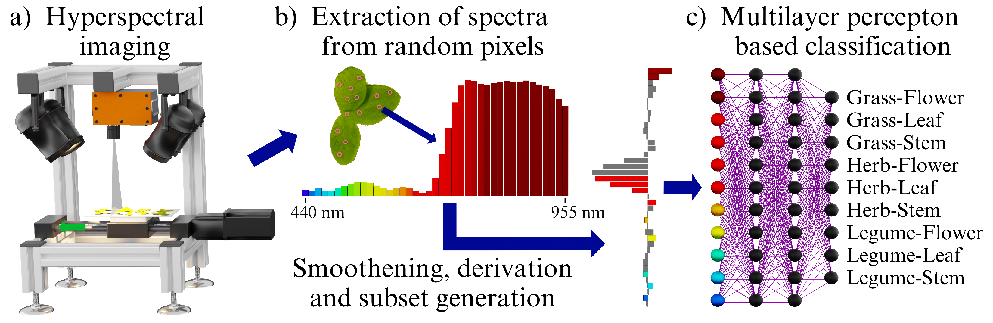
Figure 1 shows the methodical workflow of this study in a simplified version, which is described briefly here and detailed in subsequent sections. First, a sample of a specific plant part, e.g., a legume leaf or a herb flower, was recorded using a hyperspectral imaging line scanning camera. Pixels were randomly selected from the recorded sample. Their extracted spectra were smoothed with a Savitzky–Golay filter and derived.

Data processing with Savitzky–Golay filtering and with a subsequent derivation delivered the highest grassland classification accuracies in the experiments by Britz et al. [10] compared to different combinations of Savitzky–Golay filtering, derivation and Z-standardization or none of them. Datasets without additional preprocessing showed the second-best performance. In pretests, these two variants were evaluated for the combined classification of species group and plant parts, as conducted in this study. For the baseline variant, it was confirmed that additional preprocessing is beneficial (Tables S1 and S2).

In the next step of the methodical workflow, data subsets including selected predictors (spectral bands) and varying predictor counts were formed using different approaches. Finally, MLPs were trained with cross-validation to classify a combination of grasses, herbs and legumes with flowers, leaves and stems for the different approaches.

The raw dataset used throughout this study and the data preprocessing methods were previously described by Britz et al. [10]. Hence, Section 2.1, Section 2.2, Section 2.3, Section 2.4 and Section 2.5 are largely redundant.

2.1. Measurement Setup

To provide standardized laboratory conditions, an in-house hyperspectral imaging setup was used for measurements. It consisted of a line-scanning hyperspectral camera Fx10 (Specim, Spectral Imaging Ltd., Oulu, Finland) with a 12 $\mathrm{m}$$\mathrm{m}$ Cinegon 1.4/12-0906 camera lens (Schneider Kreuznach, Bad Kreuznach, Germany). Resolutions were 1024 pixels and 224 spectral bands in the range of 400 $\mathrm{n}$$\mathrm{m}$ to 1000 $\mathrm{n}$$\mathrm{m}$ (full width at half maximum (FWHM): 2.6 $\mathrm{n}$$\mathrm{m}$ to 2.8 $\mathrm{n}$$\mathrm{m}$). Illumination was provided by four 50 $\mathrm{W}$, 3000 $\mathrm{K}$ halogen light sources “GX5,3 DECOSTAR” (OSRAM GmbH, Munich, Germany), and a black shading box was used to exclude extraneous light. The sample stage with a size of $11.5$ $\mathrm{c}$$\mathrm{m}$ × 25 $\mathrm{c}$$\mathrm{m}$ was mounted onto a linear axis SHT12 with a 250 mm driving path (Igus Inc., East Providence, RI, USA) and moved by a stepper motor PD4-C5918L4204-E-08 (Nanotec Electronic GmbH and Co. KG, Feldkirchen, Germany). The camera was positioned in a nadir position at a distance of 20 $\mathrm{c}$$\mathrm{m}$ between the camera lens and the sample stage. The system was operated with in-house C++ software using the LUMO SpecSensor SDK 1.1 provided by the camera manufacturer and Qt 5.14.2 (Qt Group Plc, Helsinki, Finland) and OpenCV 4.10 (OpenCV, Great Lakes, MI, USA).

2.2. Sampling Locations

Two grassland sites, each of which was harvested three times per year, were used to obtain the plant samples for this study. The first site was the experimental field at the “Agricultural Research and Education Centre Raumberg-Gumpenstein” (Irdning, Austria, coordinates: $47.495$${}^{°}$ N, $14.100$${}^{°}$ E) where numerous grassland species were grown in monoculture (pure grass and legume stands). The second site was the “VetFarm” from the University of Veterinary Medicine, Vienna, located in Pottenstein, Austria, where three different grassland types were selected—first, an intensively used grass–clover mixture (K1: flat and moist area, coordinates: $47.960$${}^{°}$ N, $16.138$${}^{°}$ E) and second, a more extensively used permanent grassland (K2: flat and relatively dry area, coordinates: $47.960$${}^{°}$ N, $16.139$${}^{°}$ E). The third site in Pottenstein was a quite extensively used meadow (K3: relatively dry and hilly area, coordinates: $47.956$${}^{°}$ N, $16.116$${}^{°}$ E). By sampling the individual growths, species-specific differences in phenology and development during the vegetation period could be well recorded and taken into account. The sampling took place immediately before the respective harvest of the plots. Grass samples were taken at typical harvest times between the vegetation stages of “stem elongation” (E) and “anther emergence/anthesis” (R4) according to the definitions provided by Moore et al. [21]. Legumes were sampled at the vegetation stage of “inflorescence emergence/first spikelet visible” to “anther emergence, anthesis” (R1–R4). Further details regarding the dataset are provided in Table S3.

2.3. Sampling Procedure and Data Acquisition

Plants were manually picked from randomly selected positions within the sampling area, cut a few centimeters above ground level and processed immediately. Each sample was derived from an individual plant, except for the creeping plant species, for which repeated sampling might have occurred. Samples that did not fit the sample stage were cut into smaller pieces and subsequently considered as a single sample. All samples were classified according to classes formed by a combination of species group (grass, herb or legume) and plant part (flower, leaf or stem) (

Table 1. Number of samples with regard to class membership, location and seasonal cut. Each plant part (flower, leaf or stem) from a different plant per seasonal cut is considered as a sample.

			Gumpenstein			Kremesberg
Class	Species Group	Plant Part	${\mathit{n}}_{\mathbf{cut}1}$	${\mathit{n}}_{\mathbf{cut}2}$	${\mathit{n}}_{\mathbf{cut}3}$	${\mathit{n}}_{\mathbf{cut}2}$	${\mathit{n}}_{\mathbf{cut}3}$	Sum
GF	Grass	Flower	451	84	224	63	4	826
GL	Grass	Leaf	507	446	938	30	52	1973
GS	Grass	Stem	488	119	231	33	7	878
HF	Herb	Flower	0	0	0	37	20	57
HL	Herb	Leaf	0	0	0	36	115	151
HS	Herb	Stem	0	0	0	30	60	90
LF	Legume	Flower	66	112	170	34	16	398
LL	Legume	Leaf	150	146	315	45	72	728
LS	Legume	Stem	128	158	261	47	73	667
								5768

and Table S3). Class names were abbreviated by the first characters of the species group and plant part. Samples were positioned on the sample stage with the upper surface facing the camera lens. In total, 5768 samples of at least 19 grass, 6 herb and 5 legume species were acquired and processed (Table S4).

Calibration acquisitions were used to generate a radiometrically calibrated dataset. Dark calibration acquisitions were obtained by covering the lens with a lightproof lens cap using the same exposure time as the sample acquisitions. A calibrated reflection standard Zenith Lite with approximately 90% reflection (250 $\mathrm{n}$$\mathrm{m}$ to 2450 $\mathrm{n}$$\mathrm{m}$) (SphereOptics GmbH, Herrsching, Germany) was used for bright calibration acquisitions. Here, shorter exposure times compared to sample acquisitions were used to prevent overexposure of the camera chip. Dark and bright calibration acquisitions were obtained separately for each date.

2.4. Data Preprocessing

An RGB representation of each acquisition was used to manually annotate each flower, leaf or stem with polygons using the software Computer Vision Annotation Tool (CVAT) (version: server 1.1, core 2.0.1, canvas 2.0.1, UI 1.2.0) [22]. Metainformation regarding the species group, plant part, sampling site and the seasonal cut was assigned to each polygon. Pixels with intensity values of 0 or 4095 (12-bit detector) were disregarded.

Next, the dark and bright calibration median lines were calculated based on the calibration acquisitions, and defective camera sensor pixels were excluded. Starting from uncalibrated reflectance data $R_{\mathrm{UC}}$, the radiometrically calibrated reflectance $R_{\mathrm{RC}}$ for each pixel x and each wavelength $\lambda$ was calculated according to

$$R_{\mathrm{RC}}(x,\lambda )=\frac{R_{\mathrm{UC}}(x,\lambda )-D(x,\lambda )}{B(x,\lambda )-D(x,\lambda )}\times C\left(\lambda \right)$$

(1)

where D is the dark calibration median, B is the bright calibration median, and C is a specific correction factor of the reflectance standard provided by the manufacturer. Bright calibration reflectance values were corrected using a scaling factor for the differences in exposure time. Otherwise, all exposure times were identical.

The 16 lowest and highest spectral bands were removed because of the low quantum efficiency of the sensor and the low light intensity at the border areas, resulting in an effective spectral range from 440.43 $\mathrm{n}$$\mathrm{m}$ to 957.9 $\mathrm{n}$$\mathrm{m}$ and 192 spectral bands. Outliers from each sample were removed by carrying out a robust principal component analysis with two main components (the PcaHubert function from R package rrcov 1.5.5 [23]).

Next, subsampling using hierarchical clustering with the function hclust from R package fastcluster 1.2.3 [24] with complete linkage based on a Euclidean dissimilarity matrix was performed. The generated cluster tree was cut down to 10 clusters. Then, for each polygon, a total of 100 pixels was drawn, randomly stratified from the clusters. In cases in which there were 100 or fewer pixels available in total, all the pixels were drawn. However, polygons consisting of less than 95 pixels were disregarded. All polygons were grouped based on their class membership, and the dataset was split into five stratified chunks. Pixels from individual polygons were assigned to the same chunk.

A Savitzky–Golay filter (the savgol function with a filter length of 5 and a quadratic filter from R package pracma 2.3.3 [25]) was applied, followed by a derivation. As for the derived spectrum, the middle wavelength of both center wavelengths used for derivation was assigned as new name and is referred to as a predictor (Table S5), if not stated differently. The term input size refers to the number of predictors used for training and validation.

Data processing and statistical analysis were conducted using R 4.0.1 [26], especially using the R packages data.table 1.14.0 [27], dtplyr 1.1.0 [28] and tidyverse 1.3.1 [29]. Statistical significance was computed using an ANOVA using the function “aov” included in R, followed by a Tukey’s honest significance test using the function HSD.test (package agricolae 1–3.5 [30]) with a significance level $\alpha =5\%$. All parameters not explicitly mentioned were set to default values.

2.5. Multilayer Perceptron (MLP) Training

MLP networks were trained using Python 3.8.1, PyTorch 1.7.0 [31], Tune [32] included in Ray 1.0.1 [33] and hyperopt 0.2.5 [34]. The network architecture started with a fully connected layer, linking the inputs—that is, the predictors—with the first hidden layer, followed by batch normalization and a rectified linear unit activation function (ReLU). After another fully connected layer with a ReLU, the final layer was connected to the nine output classes. The class weights were normalized by the number of samples per class to compensate for the unbalanced classes. Cross-entropy loss with class weights was implemented as a loss function, together with a stochastic gradient descent optimizer. A softmax function was used during inference to convert the raw MLP output into probabilities.

Hyperparameters for each variant were searched using an “AsyncSuccessiveHalvingAlgorithm” (ASHA) included in Ray Tune as a scheduler, together with the hyperopt search algorithm. Each hyperparameter combination, selected by hyperopt out of the search space (Table S6), was trained for 100 epochs or stopped early via ASHA, which was configured with one grace period and a reduction factor of 4. In total, 200 hyperparameter combinations per variant were evaluated using dataset chunks 1 to 4 as the training dataset and chunk 5 for validation. The five hyperparameter combinations, having achieved the highest accuracy per variant, were retrained with five-fold cross-validation for 200 epochs. In this article, training always refers to the described hyperparameter search, followed by the cross-validated training of the top five combinations. The model with the highest cross-validated accuracy among the five models found at any epoch is depicted in the results, and accuracy is always shown as the mean validation accuracy. Three different evaluation metrics were used in this article, namely the mean classification accuracy (MCA), which is the mean among the classes of the mean validation accuracies; the weighted F1 score (F1) from scikit-learn 0.23.2 [35], which considers class imbalance; and finally, the absolute class accuracies. More details about the hyperparameters used in the final models are given in Table S7.

2.6. Dataset Variants

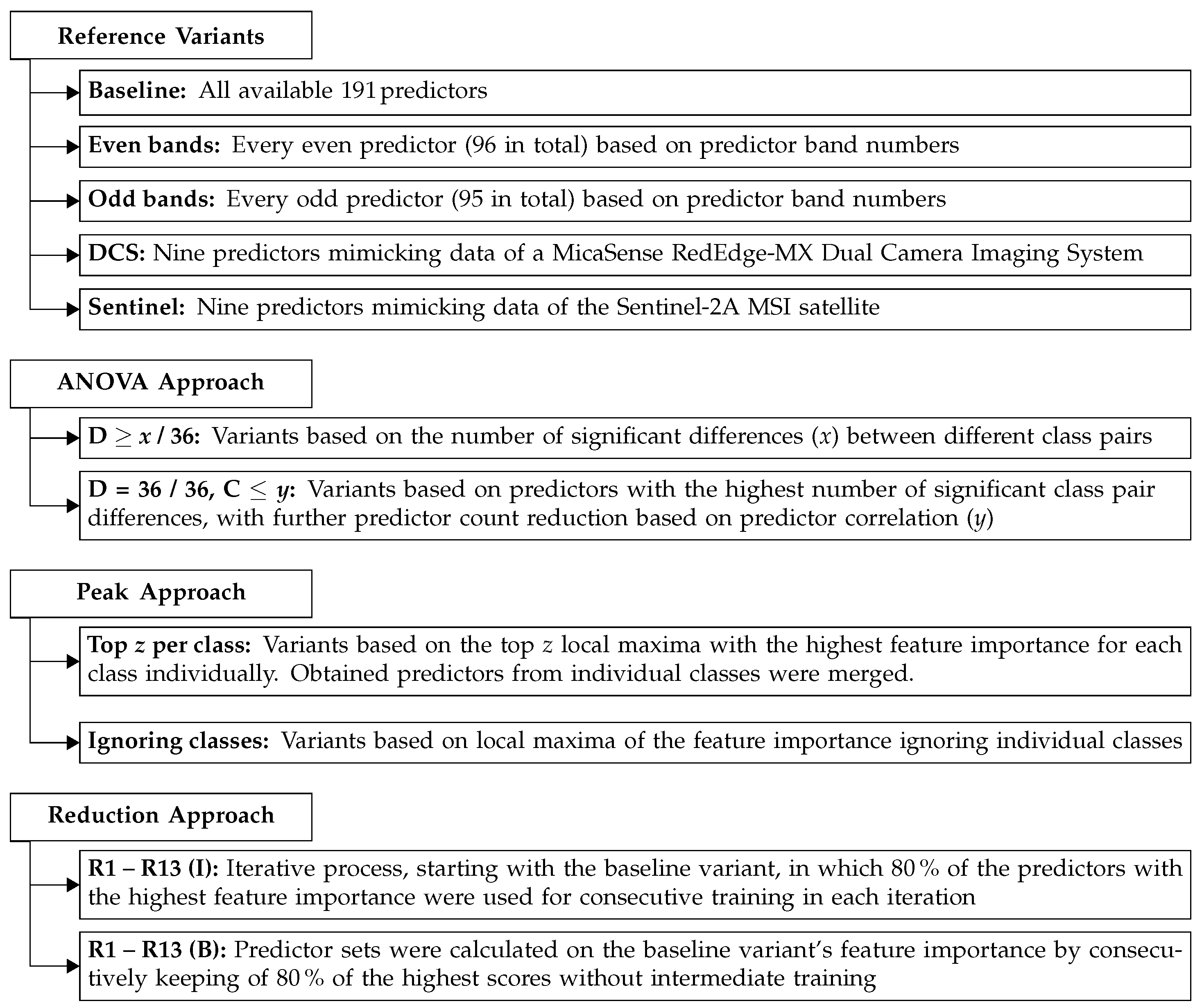
Dataset variants were grouped into the categories of reference variants, ANOVA approach, peak approach and reduction approach (Figure 2) and are explained in the following.

2.6.1. Reference Variants

A so-called baseline variant was trained, comprising all predictors to classify a combination of species group and plant part. This variant was used as a reference for all other variants. For immediate comparison, MCA was also calculated for individual models, classifying either species group or a plant part.

Further reference variants were introduced for a better understanding of the system and as a means of comparison. Two of these were variants with even and odd predictor band numbers (Table S5). Thus, the number of predictors in the models was bisected. Furthermore, two widely used sensor systems were modeled using the recorded hyperspectral data from the respective bands. The first was the “RedEdge-MX Dual Camera Imaging System” (DCS) [36]. The mimicked data covered all DCS spectral bands with their center wavelength and the full FWHM, except for the spectral band with the lowest nanometer region (

Table 2. Spectral specifications of the third-party sensor systems and the corresponding mimicked predictors (the unit of all values is nm). For Sentinel, three bands with wavelengths above 1000 nm could not be mimicked.

Third-Party Sensor			Mimicked with Fx10 Data
Center Wavelength	FWHM Lower Limit	FWHM Upper Limit	Predictor Name	FWHM-Based Lower Limit	FWHM-Based Upper Limit
DCS
444.0	430.0	458.0	449.6	439.1	460.1
475.0	459.0	491.0	474.6	457.5	491.7
531.0	524.0	538.0	531.4	523.5	539.4
560.0	546.5	573.5	559.3	544.7	574.0
650.0	642.0	658.0	650.4	641.0	659.8
668.0	661.0	675.0	667.9	659.8	676.0
705.0	700.0	710.0	704.5	697.7	711.2
717.0	711.0	723.0	716.7	708.5	724.8
740.0	731.0	749.0	739.8	730.3	749.3
842.0	813.5	870.5	842.7	812.3	873.0
Sentinel
442.7	432.2	453.2	442.7	439.1	454.9
492.4	459.4	525.4	492.4	439.1	534.1
559.8	541.8	577.8	559.8	536.7	582.0
664.6	649.1	680.1	664.6	646.4	684.1
704.1	696.6	711.6	704.1	695.0	714.0
740.5	733.0	748.0	740.5	730.3	749.3
782.8	772.8	792.8	782.8	768.5	795.8
864.7	854.2	875.2	864.7	773.9	903.5
832.8	779.8	885.8	832.8	848.1	878.6
945.1	935.1	955.1	945.1	931.4	959.3

). This band was mimicked only partly due to the insufficient spectral coverage of the Fx10 dataset. For all mimicked bands, the mean measurement value of all included spectral Fx10 bands was used as a predictor. The second sensor system was the satellite Sentinel-2A MSI (Sentinel) [37]. Sentinel data were mimicked (Table 2) using a spectral response function [38]. To apply this function, continuous non-zero data blocks of the spectral response function data were linearly interpolated to a resolution of $0.1$ $\mathrm{n}$$\mathrm{m}$ and mapped to the nearest predictor. The spectral band with the lowest nanometer region was mimicked only partly due to the insufficient spectral coverage of the Fx10 dataset. For the same reason, three spectral bands with wavelengths higher than 1000 $\mathrm{n}$$\mathrm{m}$ could not be mimicked. For comparison purposes, DCS and Sentinel variants were trained with and without the data preprocessing combination of Savitzky–Golay filtering and subsequent derivation.

2.6.2. Analysis of Variance (ANOVA) Approach

An individual one-way ANOVA (the aov function included in R 4.0.1 [26]), followed by a Tukey–Kramer test (function HSD.test from the package agricolae 1–3.5 [30] with parameters “group” set to false and “unbalanced” set to true), was performed for each predictor to analyze statistical differences between class pairs. Among the 36 pairs, the total number of class combinations having significant differences ($\mathit{p}\le 0.05$) for each predictor was calculated. The predictors with significant differences (indicated by the character D) for at least 33, 34, 35 or 36 class pairs were used to create individual subsets for training.

Predictor correlation was used for further predictor reduction based on the subset with $\mathrm{D}=36$. For this, a dataset subset with 5000 random samples per class was drawn and fed into the R function vifcor from the package usdm 1.1–18 [39]. The whole subset was used for calculation, and the maximum allowed correlation (C) was set to the thresholds 0.95 to 0.45 with steps of 0.1. The predictors remaining after using the vifcor function per threshold were used as dataset subsets and trained. This procedure resulted in 10 variants: 4 based on the ANOVA followed by the Tukey–Kramer test and 6 based on further predictor reduction utilizing correlation thresholds.

2.6.3. Peak Approach

Feature importance was analyzed using the attr.IntegratedGradients function from Captum 0.2.0 [40]. Integrated gradients (IGs) were calculated for the respective validation data. Instead of signed values, absolute IG values were utilized for further calculations. For each predictor, either the class-irrespective mean or the individual class means were calculated and used as a measure of their feature importance.

For the peak approach, IGs of the baseline model were used as input vectors to find local maxima (peaks) using the function findpeaks from the R package pracma 2.3.3 [25]). The default function parameters were kept. The minimum peak-to-peak distance was set to four predictors, and the maximum number of peaks to return was set to 100. The peak approach was split into two variations. The first used the individual class IG means. Different subsets were created using the 30, 25, 20, 15, 10, 7, 5 and 3 highest peaks per class. If the number of peaks available was lower than the number of peaks requested to form a subset, all the peaks present were included. The top n peak predictors per class were merged and used for training. The second variation, ignoring individual classes, used the IG means for peak finding, which were then used as a subset and trained.

2.6.4. Reduction Approach

The reduction approach is an iterative approach that uses the baseline variant IGs as a starting point. The IGs were calculated as described for the peak approach. A maximum of 80% of the predictors with the highest mean IGs were kept for subsequent models. With the reduced predictor set, training was conducted. For the following reduction step, newly calculated IGs based on the best cross-validated model were used as input parameters. This process went on for 13 iterations, reducing the number of predictors to 9. Each iteration was denoted by the capital character R, followed by the iteration number. Furthermore, subsets, based on a reduction directly from the baseline variant without intermediate training, were created with the same reduction factor to examine differences between a reduction with and without intermediate training.

3. Results

3.1. General Classification Performance

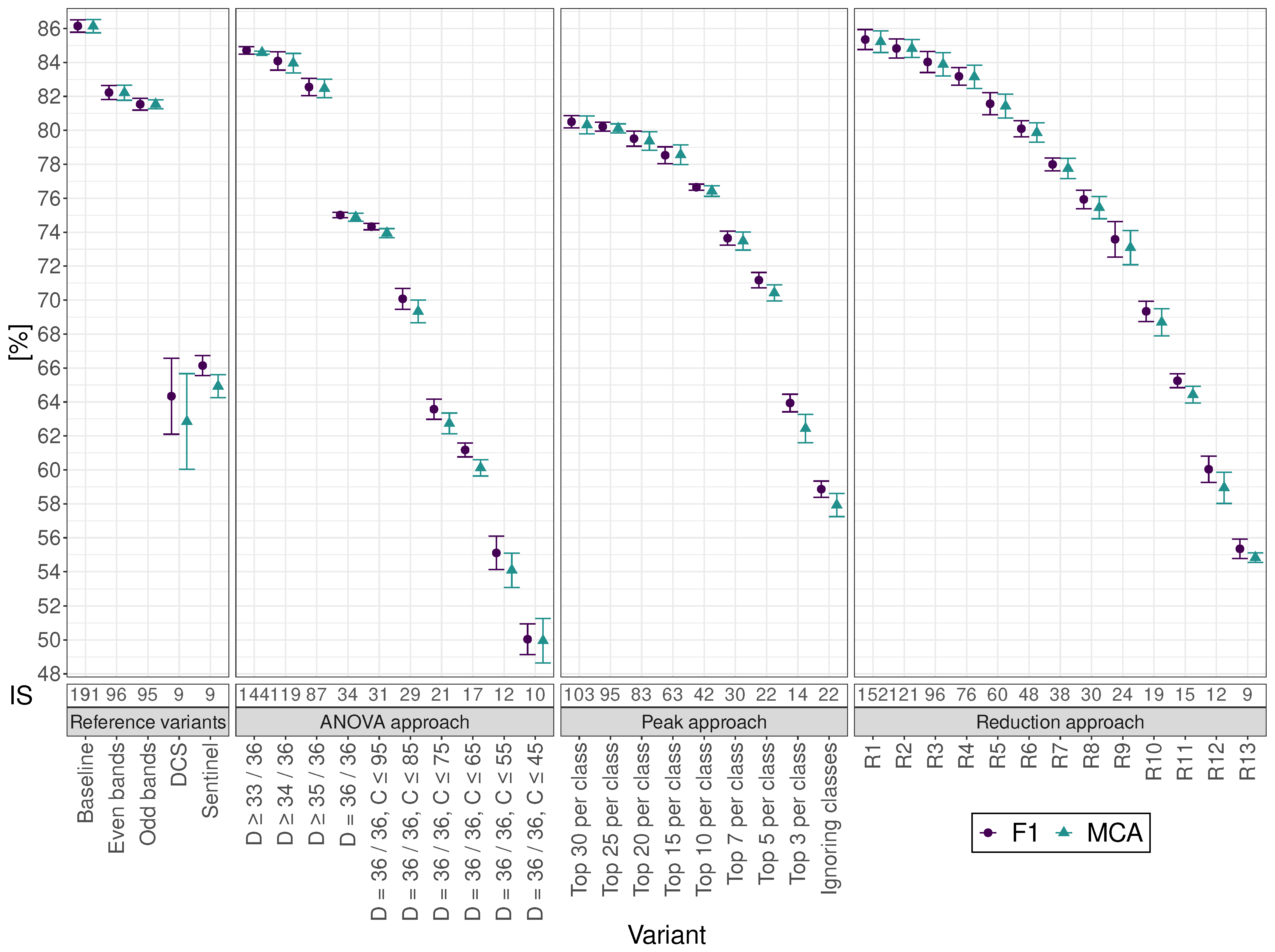
The cross-validated mean classification accuracy (MCA) and the weighted F1 score (F1) for classifying the nine different grassland classes were calculated for each variant (Figure 3 and Table S1) to compare achievable classification accuracies for the baseline variant and the different approaches with reduced predictor input sizes. The baseline variant reached an MCA and F1 of $86.1$%. Here, the manually calculated MCA values were $93.3$% for species group and $87.8$% for plant part classification. The reference variants with even and odd predictor band numbers led to a slightly reduced MCA and F1 of approximately 82% for input sizes of 96 and 95, respectively. As for the reference sensor systems, the DCS variant reached an MCA of $62.8$% and F1 of $64.3$%, whereas the Sentinel variant, with the same input size of nine, reached slightly higher values of $64.9$% for MCA and $66.1$% for F1.

In general, a similar trend could be observed for all chosen approaches: namely, reducing the input size led to a decreased MCA and F1. As no significant differences between MCA and F1 were found for any variant, only F1 is described in the following if not stated otherwise.

The reduction approach variants R1 and R2, with input sizes of 152 and 121, and the ANOVA approach variant D $\ge 33$, with an input size of 144, showed no significant differences compared to the baseline variant, with an F1 ranging from $84.7$% to $85.3$%. Therefore, an input size of 121 was sufficient to reach comparable classification performance instead of using all 191 predictors.

Regarding variants with statistically lower performance than the baseline variant, the reduction approach led to higher performance than the ANOVA and peak approach when using similar input sizes. However, comparing the latter two approaches, the ANOVA variant D $= 36$ with an input size of 34 and the peak approach top 10 variant with an input size of 42 led to non-significantly different F1 values of $75.0$% and $76.6$%, respectively. For variants with input sizes of 30 or smaller, the ANOVA approach variants performed worse compared to the peak approach variants with similar input sizes.

When comparing the reference variants DCS and Sentinel with their input size of nine and an F1 of approximately 65% to the other approaches, no significant differences between them and the reduction approach variant R11 (with an input size of 15) could be seen. In contrast to the baseline variant without Savitzky–Golay filtering and derivation, DCS and Sentinel variants without such preprocessing performed significantly better compared to the derived variants (Table S1). However, for comparability, all depicted variants include the same preprocessing steps.

The peak approach variant, ignoring classes, performed considerably worse, with an F1 value of $58.9$% compared to the top five variant with $71.2$% at the same input size of 22. Hence, it is not included in any further considerations.

The input size-reduction steps were determined based on the implemented approach. They were found to be the smoothest for the reduction approach, followed by the peak approach and the ANOVA approach, showing a distinctive gap between input sizes of 87 and 34.

3.2. Class-Based Classification Performance

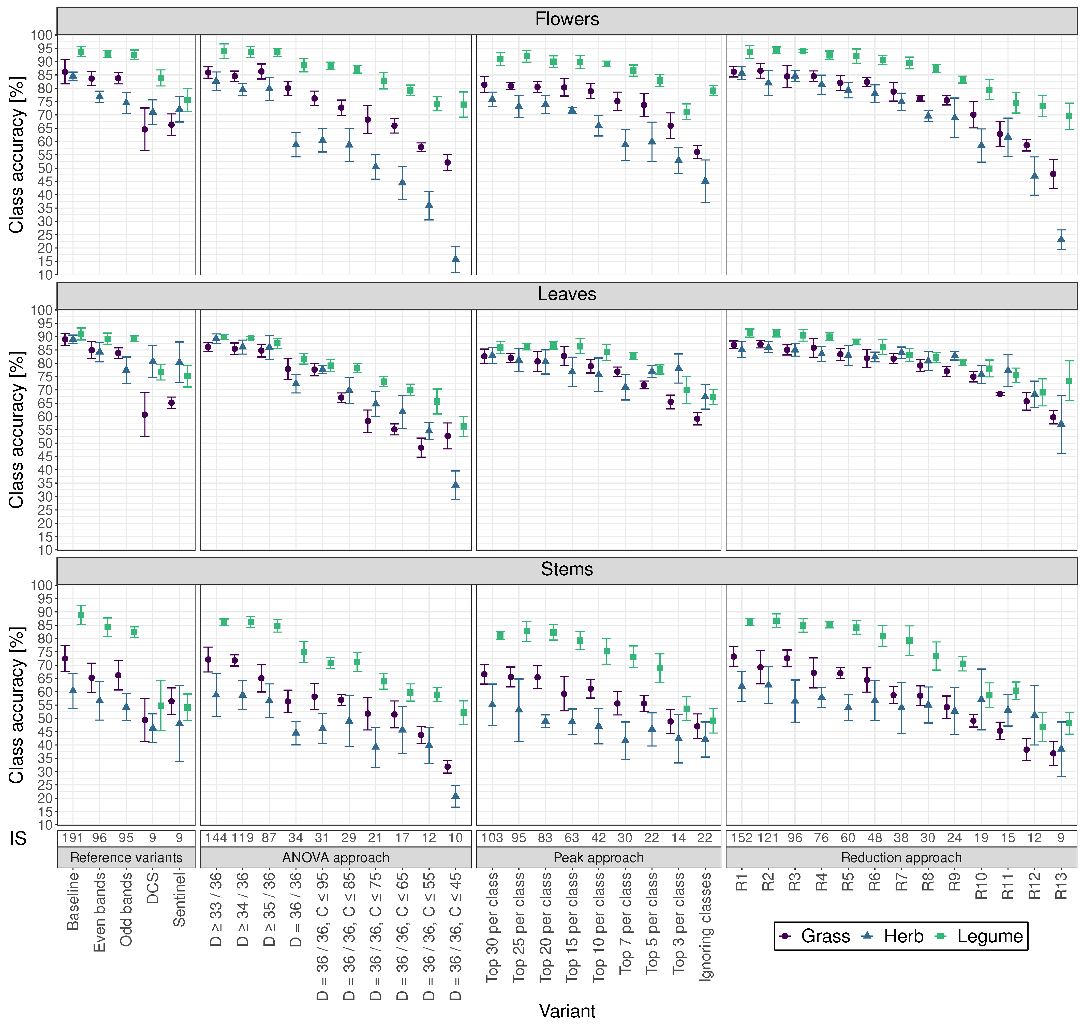
Cross-validated individual class accuracies are presented in aggregated sub-figures for flowers, leaves and stems (Figure 4 and Table S2) and are described in more detail in the following paragraph. In some classes, variants that achieved a higher accuracy than the baseline variant were found; however, these differences were not significant in any case.

For flowers, obtained baseline variant accuracies were $86.2$%, $84.6$%, and $93.7$% for the species groups grass, herb and legume, respectively. Although leaves led to similar accuracies ranging from 88.9% to 91.0%, lower values, as well as a larger variation, could be observed for stems with baseline variant accuracies of $72.5$%, $60.3$%, and $88.9$% for the species groups grass, herb and legume, respectively.

Although only about half the input size, the variant even bands showed no significant differences for all plant parts compared to their individual class baseline variants. Like the overall approach including all classes, the DCS and Sentinel variants outperformed several other variants even though they had the smallest input sizes.

For flowers, leaves, and stems, a decreasing input size led to non-significant different accuracies compared to the baseline variant the longest using the reduction approach. Taking flowers, leaves and stems together, the variant R7 led to the smallest input size of 38 without significantly losing accuracy compared to the baseline variant.

Concerning the classification accuracy distribution per variant, for leaves, there were largely no significant differences between grasses, herbs and legumes. For flowers, the variation in accuracy between grasses, herbs and legumes became larger with decreasing input size. In contrast, stems showed the opposite pattern, except for the ANOVA approach variants. For most variants, legumes reached the highest class accuracies, followed by grasses.

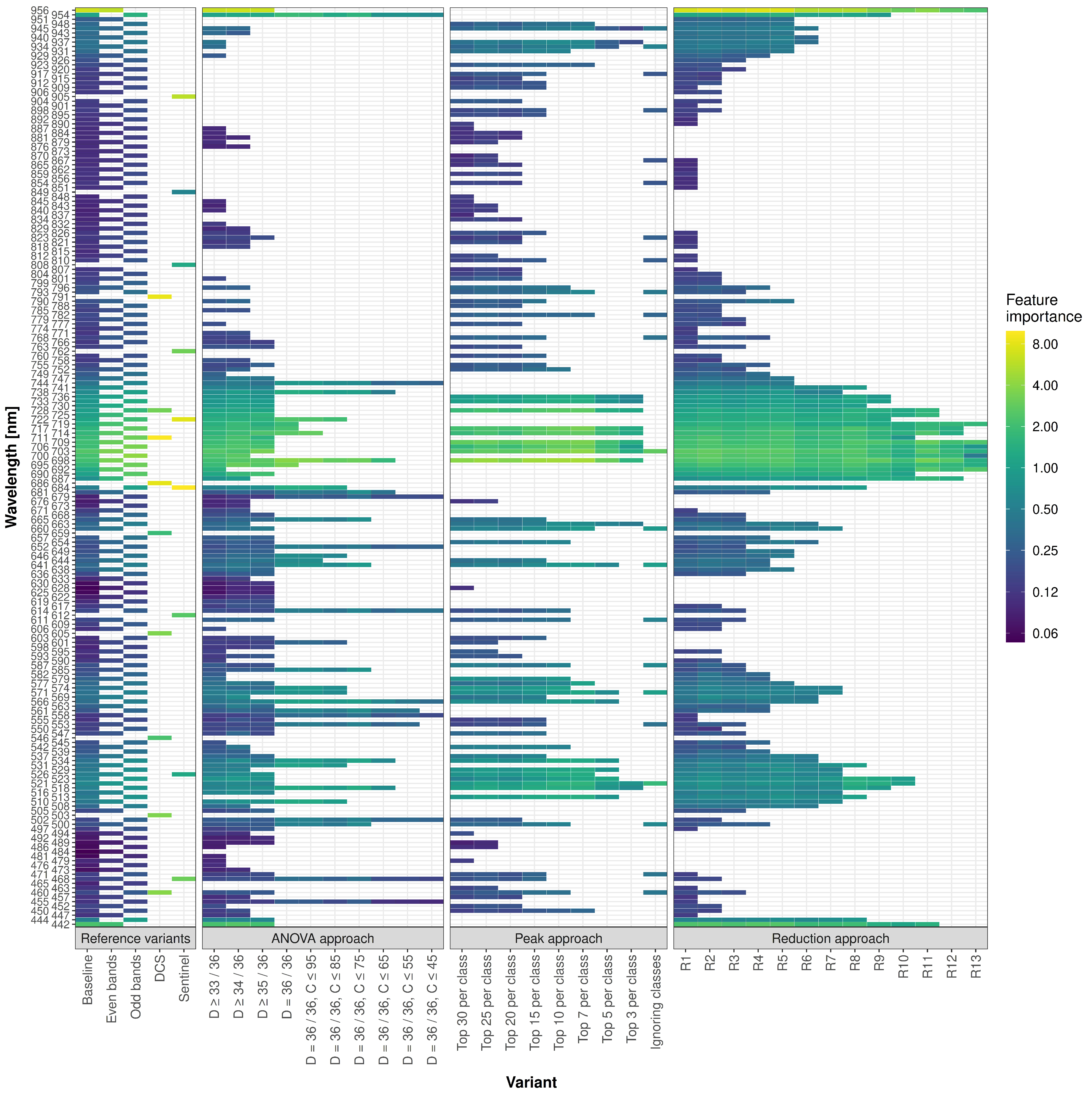
3.3. Feature Importance

In the following, the different approaches are dissected with a particular focus on predictor relevance regarding classification performance. For readability purposes, mean absolute feature importance is referred to as feature importance.

First, we examine the feature importance for each predictor, approach and variant (Figure 5). DCS and Sentinel variants reached the highest feature importance values of all variants. Still, all variants showed a similar feature importance pattern.

To identify connected regions with high feature importance, i.e., parts of the spectrum with an influence on classification performance, the value of the third quartile of the baseline variant of 0.32 was chosen as a cutoff. The resulting regions of the baseline variant cover similar spectral ranges to those of variant R6, which achieved an F1 of 80% (

Table 3. Regions of continuous predictors with a minimum absolute feature importance of 0.32 (third quartile of the baseline variant) for the variants baseline and R6. Single predictors not connected to a continuous region were included. PR = predictor range [nm], $n_{\mathrm{P}}$ = number of predictors, FI = feature importance.

Baseline			R6
PR [nm]	${\mathit{n}}_{\mathbf{P}}$	FI	PR [nm]	${\mathit{n}}_{\mathbf{P}}$	FI
442–444	2	2.21	442–444	2	1.82
510–534	10	0.61	508–537	12	0.67
566–577	5	0.39	566–574	4	0.54
			654	1	0.34
			660–663	2	0.49
684–744	23	2.44	684–741	22	2.15
931–945	6	0.37	937	1	0.35
			945	1	0.48
954–956	2	6.78	954–956	2	5.93

). The predictors 954 $\mathrm{n}$$\mathrm{m}$ to 956 $\mathrm{n}$$\mathrm{m}$ showed approximately three times the feature importance of the second-most important region 684 $\mathrm{n}$$\mathrm{m}$ to 744 $\mathrm{n}$$\mathrm{m}$ for the baseline variant and 684 $\mathrm{n}$$\mathrm{m}$ to 741 $\mathrm{n}$$\mathrm{m}$ for R6, respectively. A third region from 442 $\mathrm{n}$$\mathrm{m}$ to 444 $\mathrm{n}$$\mathrm{m}$ showed a feature importance that is worth pointing out. However, all other ranges or predictors identified are of minor importance. In general, the predictors of the baseline variant and R6 found were identical or showed only slight deviations. Interestingly, for R6, the predictors 654 $\mathrm{n}$$\mathrm{m}$ to 663 $\mathrm{n}$$\mathrm{m}$ were present, whereas for the baseline variant, no predictors close to this region were included. Regarding the spectral width, the second-most important feature importance region around 684 $\mathrm{n}$$\mathrm{m}$ to 744 $\mathrm{n}$$\mathrm{m}$ with 23 pedictors was the widest, followed by the region around 520 $\mathrm{n}$$\mathrm{m}$ with roughly half the size. All other regions were built upon six or fewer connected predictors.

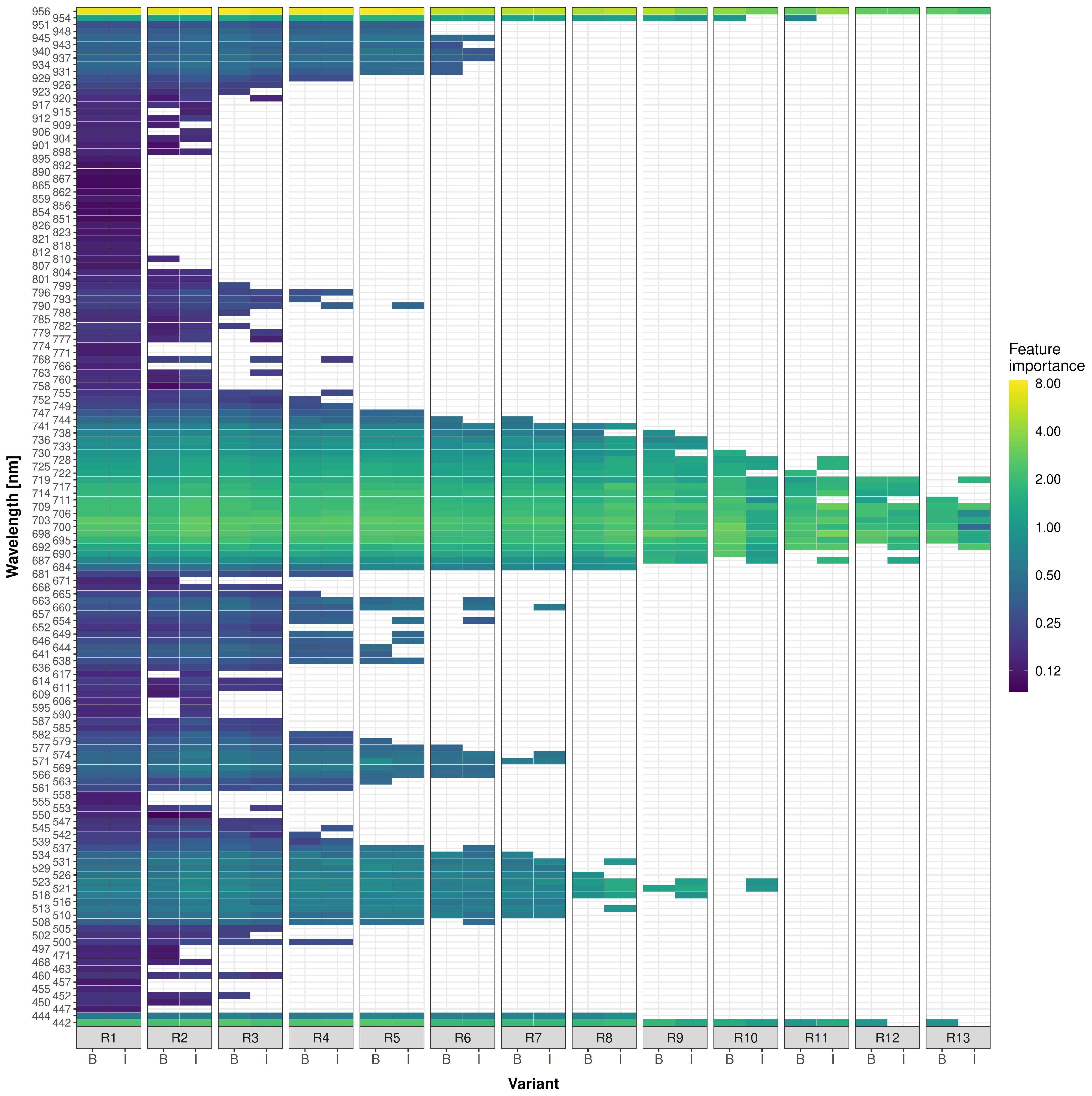
Next, the results of the reduction approach are examined in more detail (Figure 6 and Table S8). Compared to a direct reduction (B), where all further subsets emanated solely from the baseline variant’s feature importance values, the reduction with intermediate training (I) for obtaining new IGs showed no significant F1 differences. Exceptions were R10, R11 and R12, with approximately 3% lower performance for the directly reduced variants, meaning that predictors chosen directly from the baseline variant varied only slightly compared to variants with intermediate training, even at higher reduction steps. Furthermore, even the feature importance values showed only slight variations between B and I-variants.

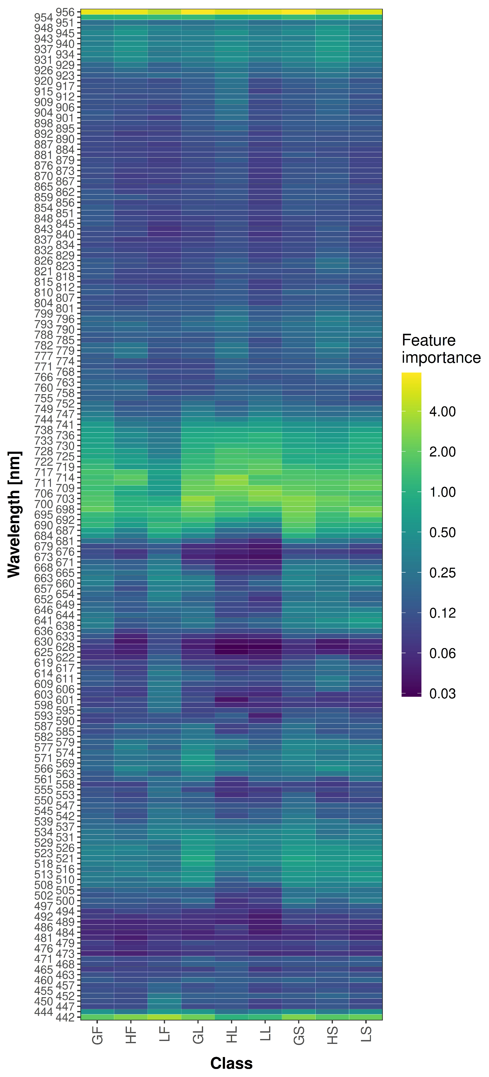
The bases for the peak approach were class-dependent feature importance values (Figure 7). The feature importance values generally showed similar behavior for the different classes per predictor. Only a few predictors, such as 601 $\mathrm{n}$$\mathrm{m}$, showed higher variations in the feature importance values per class. The identified and selected peak predictors can be found in Figure 5 and in greater detail with the different class contributions in Figure S1.

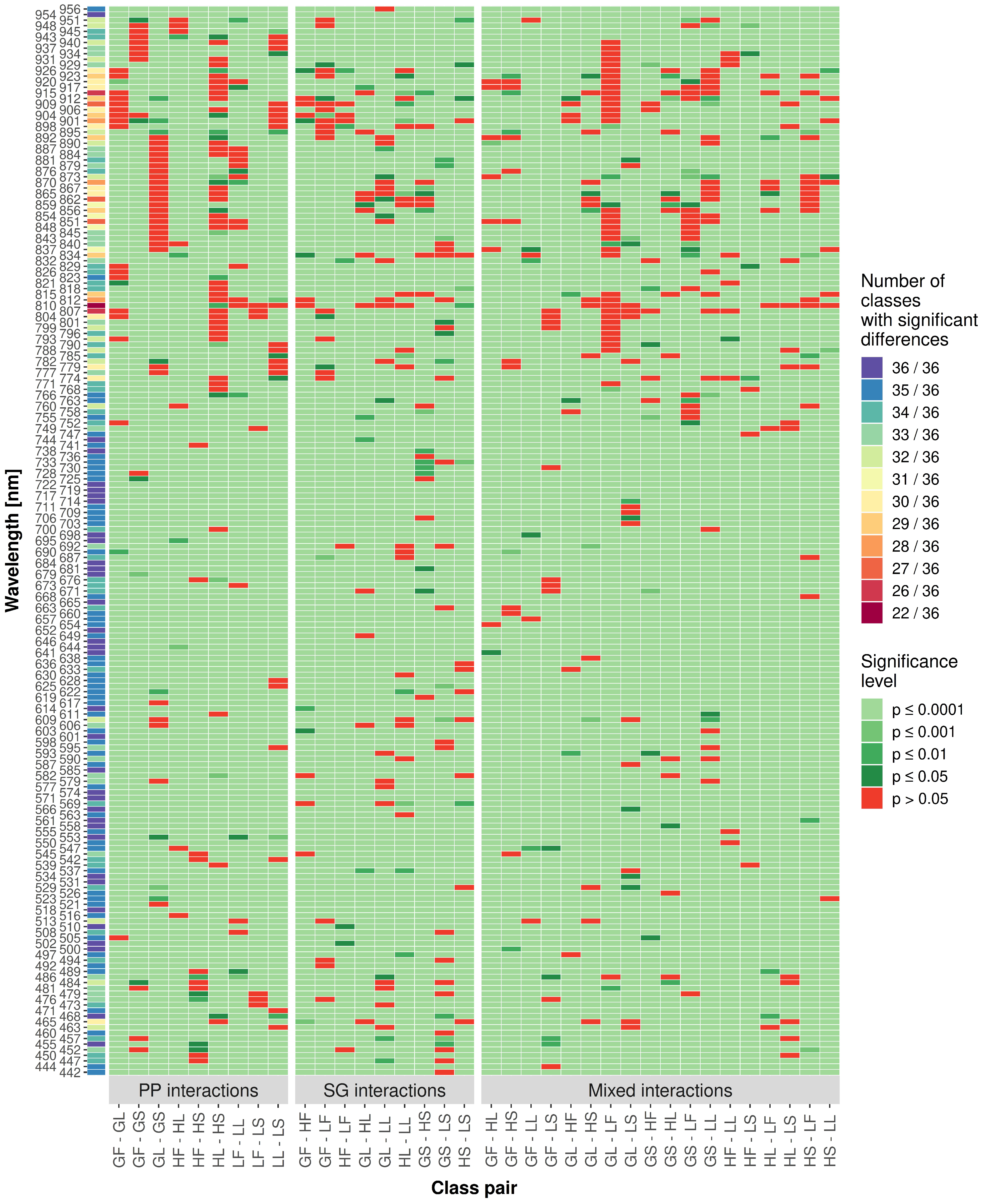
As an alternative method to examine the grassland classification potential of each predictor, an ANOVA followed by a Tukey–Kramer test was conducted on the dataset used for training the baseline variant (Figure 8). For each predictor, all class pairs were tested for significant differences to learn about classification contribution potential. The figure was split into different parts, showing interactions with the same species group and the same plant part and mixed interactions. Furthermore, the sum of the 36 distinct class pairs showing significant differences per predictor was used as a measure of overall grassland classification potential. The values of significantly different class pairs per predictor ranged from 22 to 36. The region 489 $\mathrm{n}$$\mathrm{m}$ to 766$\mathrm{n}$$\mathrm{m}$ showed high sums of class pairs with significant differences, whereas the predictor region 768 $\mathrm{n}$$\mathrm{m}$ to 951 $\mathrm{n}$$\mathrm{m}$ had the least significant differences in total. Another region with lower average counts on significant class pair differences was between 447 $\mathrm{n}$$\mathrm{m}$ to 486 $\mathrm{n}$$\mathrm{m}$. As described for the baseline variant (Table 3), the predictors located at the spectral end-regions of the dataset showed a high number of class pairs with significant differences. Over the whole predictor range, most statistically non-significant differences were found for the class pairs grass leaf–legume flower, herb leaf–herb stem and grass leaf–grass stem.

4. Discussion

Comparing the obtained baseline variant MCA of $93.3$% and $87.8$% for species group and plant part classifications to the MCA previously achieved by Britz et al. [10] by using separate classifiers for species group and plant part, a slight decrease in classification performance of $-3.6$% for species group and of $-0.8$% for plant part was identified. The MCA for the combined classifier of $86.1$% (Figure 3 and Table S1) was lower compared to separated classifiers, as with a higher class count, the probability of errors increases.

In comparison, Suzuki et al. [9] used hyperspectral imaging to classify grassland plants into the groups of perennial ryegrass, white clover and other plants, together with linear discriminant-based sequential models, based on a step-wise predictor selection algorithm. They reached an overall accuracy of $80.3$%, classifying only three different classes. The decreased performance compared to the results presented here underlines the suitability of MLPs for grassland classification.

Regarding classification performance, stems in particular lowered the total classification power (Figure 4 and Table S2). A possible reason for this decreased performance might be leaf sheaths covering stems [10] as corresponding class-pairs often showed non-significant differences (Figure 8). Knowledge about this functional plant part might be beneficial for a more in-depth analysis of grassland vegetation structures, e.g., by calculating the visible-stems-to-leaves ratio. However, when looking at grassland vegetation, only a small proportion of stems is visible compared to leaves and flowers. To increase the classification power for leaves and flowers, it might be advantageous for practical applications to ignore stems as such and assign them to a miscellaneous class. Comparing the ANOVA approach variants “D $\ge 36$, C $\le 95$”, “D $\ge 36$, C $\le 85$” and the reduction approach variant R8 with input sizes of 31, 29 and 30 (Figure 3 and Table S1), the ANOVA variants have only seven and six predictors, respectively, with R8 in common (Figure 5). Non-significant differences between the variants “D $\ge 36$, C $\le 95$” and R8 emphasize that, even with distinct differences in selected predictors, comparable accuracies can be achieved. However, even with a similar number of predictors, the predictors themselves can have a significant influence. The variant “D $\ge 36$, C $\le 85$”, with a decreased input size of either one or two compared to the other two variants, demonstrated a significantly decreased F1. Hence, the inclusion or exclusion of even one predictor in the modeling process could lead to significant differences in classification performance.

Regarding measures used to assess classifications, MCA and F1 could be used interchangeably for the presented dataset as no significant differences between these measures were found. This underlines that the cross-entropy loss function in conjunction with class weights led to classifiers taking class imbalance into proper consideration.

4.1. Comparison of Predictor Reduction Approaches

As for the predictor reduction approaches, the underlying assumption for the peak approach that each peak, i.e., each local maximum, encodes different biological information (and thus the question of whether these peaks are sufficient as predictors for grassland classification) could not be confirmed. Nevertheless, the analysis of the individual feature importance values for classification based on individual classes (Figure 7) used in the peak approach provided exciting insights. In general, all predictors contributed similarly with regard to the different classes. A reason for the deviations might be multicollinearity, which is usually present in hyperspectral data [12,41]. Comparing these results to the baseline variant (Figure 5), as well as to the results of the ANOVA approach (Figure 8), it can be seen that regions with high feature importance values correspond to areas with a high amount of significantly different class pairs. This underlines the capability of an ANOVA to identify predictors with high classification potential to be used in MLP training. However, the formation of subsets via the elimination of predictors with high correlations seems to be detrimental with regard to the reachable classification accuracy.

In general, the reduction approach (Figure 6 and Table S8) led to the highest classification performance with decreased predictor sets and thus is the recommended approach. The variants with intermediate training showed slight variation regarding the distribution of feature importance values. This underlines that all trained MLPs stably chose the same features. The often non-significant differences observed between variants with intermediate training and reduction based solely on the baseline variant strengthen the stability aspect. With limited time and machine learning resources, the formation of subsets based on the baseline variant might be sufficient, although the reduction approach with intermediate training tends to improve performance. The slight fluctuations might be attributed to collinearity between predictors.

The results indicate that the usage of at least 48 predictors is necessary to obtain an F1 score of ≥80%. However, for classification of either species group or plant part, fewer predictors might be sufficient. Comparing the even and odd variants to the baseline variant shows that even slight spectral gaps of a few nanometers, introduced by skipping every second predictor, led to significantly decreased accuracy. This indicates that even consecutive predictors, which might show high multicollinearity, are important for achieving high classification accuracies. This is further underlined by the results of the correlation-based reduction in the ANOVA approach.

4.2. Influence of Predictor Width

For the particular dataset used in this article, DCS and Sentinel showed similar feature importance distributions compared to the baseline variant. Due to the comparably wide spectral bands and distances of the DCS and Sentinel predictors, a derivation of the spectrum is not recommended, as performance decreased significantly compared to underived data (Table S1). In particular, these underived data showed a comparably high performance considering their predictor count of only 10. Nevertheless, the derived dataset undergoing the same preprocessing as all other variants with only 9 predictors also reached a non-significantly different F1 value compared to the reduction variant R11 with an input size of 15. This result shows that narrow-band predictors are not necessarily beneficial compared to wider predictors. Cundill et al. [42] achieved similar results using spectral indices, as in some cases, broad spectral bands performed better in contrast to narrow-band sensors. Nevertheless, hyperspectral sensors with narrow and near-continuous spectra facilitate better granularity compared to broadband sensors [43]. This granularity allows for more detailed and universal scientific analyses. In the end, predictor selection, including predictor width, is an optimization problem. Wide predictors might include unimportant information and decrease predictor usability. In contrast, predictors that are narrow and close to each other might encode identical information due to the multicollinearity usually present in high-dimensional data [41]. Further research is required to examine and identify predictor classification potential with regards to different subsets, including different predictor widths.

4.3. Predictor Regions with High Grassland Classification Potential

The contribution of individual predictors to classification performance might indicate biological properties encoded in different spectral regions. The predictor region with the highest grassland classification contribution was at 954 $\mathrm{n}$$\mathrm{m}$ to 956 $\mathrm{n}$$\mathrm{m}$. A similar range was identified by Sims and Gamon [44], who measured in the spectral range of 350 $\mathrm{n}$$\mathrm{m}$ to 2500 $\mathrm{n}$$\mathrm{m}$. The identified range correlates well with the water content of the photosynthetic tissue area. Furthermore, next to water accumulation, the index of refraction inhomogeneities such as interfaces due to cell membranes are encoded in this spectral region [45].

In contrast to the NIR spectral region, reflectance in VIS is mainly influenced by chlorophyll pigments [46]. The second-most important region for classification was 684 $\mathrm{n}$$\mathrm{m}$ to 744 $\mathrm{n}$$\mathrm{m}$, situated in the red and the red-edge region. Thenkabail et al. [47] mention the spectral band $682.0 \mathrm{n}\mathrm{m}\pm 2.5$ $\mathrm{n}$$\mathrm{m}$, encoding biophysical information such as leaf area index, wet and dry biomass and crop type. The bands $705.0 \mathrm{n}\mathrm{m}\pm 2.5$ $\mathrm{n}$$\mathrm{m}$ and $720.0 \mathrm{n}\mathrm{m}\pm 2.5$ $\mathrm{n}$$\mathrm{m}$ contain information regarding plant stress and chlorophyll, and in particular, the first-order derivative over 700 $\mathrm{n}$$\mathrm{m}$ to 740 $\mathrm{n}$$\mathrm{m}$ encodes chlorophyll content, senescence, stress and drought [47]. Other important regions found in the results, specifically, 442 $\mathrm{n}$$\mathrm{m}$ to 444 $\mathrm{n}$$\mathrm{m}$ and 508 $\mathrm{n}$$\mathrm{m}$ to 537 $\mathrm{n}$$\mathrm{m}$, encode chlorophyll and carotenoid content [47,48]. Due to the positions of the first and third-most important spectral regions at the respective ends of the spectral coverage of the dataset, it remains unclear whether these regions would have continued using a wider spectral coverage.

So far, the spectral properties of plants in general have been considered. However, the density of information in grassland research is limited, especially with regard to spectral classification. Arafat et al. [16] identified the spectral region of 727 $\mathrm{n}$$\mathrm{m}$ to 1299 $\mathrm{n}$$\mathrm{m}$ for the isolation of clover from wheat. Furthermore, Suzuki et al. [9] identified the regions of 420 $\mathrm{n}$$\mathrm{m}$ to 580 $\mathrm{n}$$\mathrm{m}$ and 716 $\mathrm{n}$$\mathrm{m}$ to 853 $\mathrm{n}$$\mathrm{m}$ to be suitable for classifying grassland plants into the groups of perennial ryegrass, white clover and other plants. The results of both sources agree with those shown here, although the algorithms and classes differ. Nevertheless, the results presented in this article provide deeper insights and important indications for further research.

5. Conclusions

The mean cross-validated classification accuracy and weighted F1 score of $86.1$% for classifying a combination of species group (grass, herb, legume) and plant part (flower, leaf, stem) proves the suitability of the chosen method for classifying grassland under laboratory conditions. For this, an MLP-based classifier was used on a dataset with 192 spectral bands in the range of approximately 440 $\mathrm{n}$$\mathrm{m}$ to 960 $\mathrm{n}$$\mathrm{m}$ after a smoothening operation and first-order derivation was applied. An even higher predictive performance could be reached in the classification of species groups alone.

The reduction approach with intermediate training showed the best performance for reducing the number of predictors. With limited machine learning resources, predictor reduction with this approach, solely based on the baseline variant (trained on all 191 available spectral bands), can reach comparable accuracies. With the spectral narrow band predictors (full width at half maximum 2.6 $\mathrm{n}$$\mathrm{m}$ to 2.8 $\mathrm{n}$$\mathrm{m}$), at least 48 predictors were necessary to obtain a mean cross-validated classification accuracy and a weighted F1 score of approximately 80%. Therefore, hyperspectral sensors seem to be necessary for spectral-based grassland classification with decent performance. However, fewer but spectrally wider predictors could possibly be sufficient for achieving a similar performance. Further research is necessary in this regard.

Based on the spectral range covered in this article, a sensor coverage of the particular predictor regions of 954 $\mathrm{n}$$\mathrm{m}$ to 956 $\mathrm{n}$$\mathrm{m}$, 684 $\mathrm{n}$$\mathrm{m}$ to 744 $\mathrm{n}$$\mathrm{m}$ and 442 $\mathrm{n}$$\mathrm{m}$ to 444 $\mathrm{n}$$\mathrm{m}$ for grassland classification is recommended. Further important regions were 931 $\mathrm{n}$$\mathrm{m}$ to 945 $\mathrm{n}$$\mathrm{m}$, 654 $\mathrm{n}$$\mathrm{m}$ to 663 $\mathrm{n}$$\mathrm{m}$, 566 $\mathrm{n}$$\mathrm{m}$ to 577 $\mathrm{n}$$\mathrm{m}$ and 510 $\mathrm{n}$$\mathrm{m}$ to 534 $\mathrm{n}$$\mathrm{m}$. As mentioned, all predictors are based on the derived spectrum and therefore include information from a larger spectral range (Table S5). Extending the sensor’s spectral range might lead to the identification of further important regions and improve classification performance.

This article provides an essential basis for high-performing spectral-based permanent grassland classification and the relevant spectral regions. Potential fields of applications are estimating nitrogen fertilizer needs based on legume proportion, monitoring the botanical composition for reseeding or crop protection measures and evaluating the forage quality on a small scale to improve feed efficiency. Nevertheless, the influence of site and environment conditions, species differentiation, illumination, 3D sward structure, spectrally mixed pixels and predictor width still require further research.