A Novel Object Detection Model Based on Faster R-CNN for Spodoptera frugiperda According to Feeding Trace of Corn Leaves

Abstract

The conventional method for crop insect detection based on visual judgment of the field is time-consuming, laborious, subjective, and error prone. The early detection and accurate localization of agricultural insect pests can significantly improve the effectiveness of pest control as well as reduce the costs, which has become an urgent demand for crop production. Maize Spodoptera frugiperda is a migratory agricultural pest that has severely decreased the yield of maize, rice, and other kinds of crops worldwide. To monitor the occurrences of maize Spodoptera frugiperda in a timely manner, an end-to-end Spodoptera frugiperda detection model termed the Pest Region-CNN (Pest R-CNN) was proposed based on the Faster Region-CNN (Faster R-CNN) model. Pest R-CNN was carried out according to the feeding traces of maize leaves by Spodoptera frugiperda. The proposed model was trained and validated using high-spatial-resolution red–green–blue (RGB) ortho-images acquired by an unmanned aerial vehicle (UAV). On the basis of the severity of feeding, the degree of Spodoptera frugiperda invasion severity was classified into the four classes of juvenile, minor, moderate, and severe. The degree of severity and specific feed location of S. frugiperda infestation can be determined and depicted in the frame forms using the proposed model. A mean average precision (mAP) of 43.6% was achieved by the proposed model on the test dataset, showing the great potential of deep learning object detection in pest monitoring. Compared with the Faster R-CNN and YOLOv5 model, the detection accuracy of the proposed model increased by 12% and 19%, respectively. Further ablation studies showed the effectives of channel and spatial attention, group convolution, deformable convolution, and the multi-scale aggregation strategy in the aspect of improving the accuracy of detection. The design methods of the object detection architecture could provide reference for other research. This is the first step in applying deep-learning object detection to S. frugiperda feeding trace, enabling the application of high-spatial-resolution RGB images obtained by UAVs to S. frugiperda-infested object detection. The proposed model will be beneficial with respect to S. frugiperda pest stress monitoring to realize precision pest control.

1. Introduction

Spodoptera frugiperda is a polyphagous pest species that spreads rapidly due to its wide adaptability and strong reproductive capacity and seriously affects the yield of major food crops such as maize and rice [1]. Originating in the American continent, S. frugiperda has now spread to Africa and Eurasia, causing global declines in the yield of crops such as maize [2].

In agriculture, manual field sampling is generally used to assess plant diseases and insect pests. However, data obtained via sampling sometimes do not reflect the actual situation in the field due to the randomness of the sampling and limited sample costs. Agricultural workers or experts with sufficient agronomic knowledge and experience can provide accurate diagnostic results and advice for pest control by observing images of symptomatic crops. Although clear images on a large enough scale can be obtained, manual visual diagnosis is time consuming and laborious. Moreover, it is difficult to quantify the overall distribution and degree of crops affected by pests and diseases [3]. This can lead to problems such as over-spraying, which decreases crop quality and increases production costs [4,5].

In this context, there is an urgent demand for low-cost, high-efficiency, and high-accuracy methods that can provide accurate pest field information such as the occurrence location, degree of severity, and overall distribution. The continuous advancement of machine learning and sensor technologies shows there is great potential for applying image-based models for the classification and detection of insect pests and crop diseases [6]. Liu et al. used a maximally stable extremal region descriptor to simplify the images of aphids with a complex field background, histograms of oriented gradient features and a support vector machine were then used to identify and count the aphids in the simplified images; 86.91% of mean identification was achieved by the method [7]. Hayashi et al. used auto machine learning methods to recognize three species of pest aphid and recorded and compared the performances of the machine learning methods using different amounts of training samples [8]. Wen et al. used five machine learning methods to classify global and local features of photos of orchard insects, verifying the advantages of a combination of global and local features [9]. Wang et al. segmented whiteflies on the leaves of pepper, corn, and tomato in three steps, i.e., block processing for images, K-means cluster using adaptive initial cluster center learning, and leaf veins removal. The number of whiteflies could be counted and the mean error rate was 0.0364 [10].

Furthermore, great effort is required in terms of selecting features when using classical machine learning models, while a convolutional neural network (CNN) can automatically extract image features [6].

Several recent studies have successfully applied deep learning methods, particularly CNN models, in the detection of plant diseases and insects using red–green–blue (RGB) images. Many of these studies were based on the Plant Village dataset [11,12,13,14]. However, the leaves and other parts of a plant are separate in the images of the Plant Village dataset and were photographed in a uniform laboratory background, which may not be suitable for actual production scenarios. Therefore, several research teams have collected their own images under actual agricultural conditions [15,16,17,18]. Cheng et al. improved the plain convolutional network such as AlexNet and VGGNet by deep residual learning, and 10 species of pest images with a complex field background could be distinguished at the accuracy value of 98.67% [19]. Labaña et al. developed a prototype pest recognition system using CNN and restful services, and the system was accessible to multiple types of terminals [20]. Li et al. collected ten types of crop insect images excluding the background noise, and obtained a recognition accuracy of 98.91% using fine-tune strategy with pre-train weight GoogleNet [21]. A pest objection model based on CNN was proposed by Wang et al., where a contextual information mechanism module integrating rough classification results and a multiple dimension projection module solving the problem of features disappearing in the pest detection were proposed [22]. Fuentes et al., combining a feature extractor such as VGGNet, a residual learning network, and an object detection detector such as Faster R-CNN, verified the performance of the proposed architecture on a tomato pest and disease dataset [23]. In order to solve the problems of false positive and unbalanced class occurring in pest detection studies, a refinement filter bank for tomato pest and disease recognition was proposed by Fuentes et al. [24].

Using images to determine the pest and plant disease situation does not require the transfer of plant tissue or insects to the laboratory and images, which can be acquired directly without causing damage to the plant. However, the acquisition of the large number of images required by CNN models is a time- and energy-consuming task. Therefore, a rapid, efficient, and low-cost automated platform is required to acquire adequate images.

Remote sensing, as a fast, efficient, and non-destructive image acquisition technology, has been widely used in the detection of diseases and insect pests [25,26,27,28]. There have been several classical cases of wide-scale prediction and the monitoring of plant diseases and insect pests through remote sensing vegetation indices. Through vegetation indices, diseases and insect pest information (e.g., the region and area of occurrence) can be obtained [29,30].

Lehmann et al. used high-resolution unmanned aerial vehicle (UAV) images of tree canopy to monitor splendor beetle (Agrilus biguttatus) infestation. Normalization vegetation indices were extracted from images processed with image mosaic and registration, and object-oriented classification was carried out to discriminate five types of healthy classes [31]. Escorihuela et al. applied soil moisture information included in the SMOS satellite imageries for desert locust management; soil moisture product at 1 km will be integrated into the national and global Desert Locust early warning system at DLIS-FAO [32]. Gómez et al. extracted new environment variables, i.e., surface temperature, leaf area index (LAI), and soil moisture root zone, from SMAP satellite remote sensing imageries; machine learning methods such as a generalized linear model and random forest combined with a species distribution model were used to map the distribution zones of desert locust, and a Cohen’s kappa (KAPPA) and true skill statistic (TSS) value of 0.901 and receiver operating curve (ROC) value of 0.986 were obtained in detecting the probability of desert locust presence [33]. Arjan et al. monitored the mortality situation of trees infested by bark beetles by single-date and multi-date Landsat images. The maximum likelihood classification method was conducted for single-date images and the time series of spectral indices method was conducted for multi-dates images; the classification result showed that the multi-date method is better [34]. Such methods can solve problems of quantifying the occurrence of diseases and insect pests over large areas of cropland in some sense [35].

Remote sensing data are mostly used for pre-monitoring the overall situation on a large scale. The above studies mostly focus on either provincial or municipal levels while there are limited studies concerned about agricultural pests at the precise field scale.

In recent years, significant progress has been made in UAV remote sensing technology and machine learning, especially deep learning. The combined application of both techniques has undoubtedly led to new possibilities for the precision monitoring of agricultural pests or diseases [36]. Several studies have examined the application of small UAV remote sensing to the detection of diseases and insect pests. Everton et al. applied UAV remote sensing to monitor foliar diseases and insect pests that affect soybeans [37]. Wu et al. used UAV images to monitor maize leaf blight, a low-altitude UAV was used to acquire high-resolution maize images at the flight height of 6 m, a maize leaf blight monitoring model based on the ResNet-34 model was established, and an accuracy value of 95.1% was achieved [38]. Chu et al. developed a pest detection UAV system based on the histogram of oriented gradient (HOG) and SVM algorithms [39]. Roosjen et al. used deep CNN to detect and count male and female spotted wing drosophila (SWD) occurring in images of insect traps taken in the field. Areas under the precision recall curve (AUC) of 0.506 and 0.603 were obtained for female and male SWD, respectively. The potential of insect object detection of insect trap images taken by UAV was further verified by the study [40].

In conclusion, compared with satellite remote sensing images, small UAVs have the advantages of lower application costs, higher spatial resolution, and are well suited to obtain the high-throughput images required for monitoring crop diseases and insect pests [41,42].

To the best of our knowledge, the application of UAV images for monitoring the invasion of maize by S. frugiperda has not been studied in the actual production environment and is mainly in the exploratory stage. The life cycle of S. frugiperda larvae is generally divided into six instars, during which the leaves, stems, branches, and reproductive organs of plants are damaged. For maize S. frugiperda, the first, second, and third stage of instar eat on a single side of the epidermal layer of leaf tissue while not affecting the lateral leaves, resulting in a translucent film of “silver windows” on the leaves, while other stages of larvae feed on the entire leaf layer, generating more obvious holes and causing leaf margins to be missing. In addition, the larvae of S. frugiperda are usually hidden on the back of leaves and are therefore difficult to detect directly [43]. According to the characteristics of S. frugiperda invasion, directly monitoring S. frugiperda using UAV imageries is infeasible; in order to monitor the occurrences of S. frugiperda, the significantly distinguishable silver windows and maize leaf holes, suggesting the presence of feeding S. frugiperda, were utilized as the main characteristics to indicate the presence and distribution of the larvae in maize fields.

With the powerful ability of deep learning object detection and the rapid field information accusation ability of UAV remote sensing, Pest Region-CNN (Pest R-CNN) was proposed based on Faster R-CNN in this study. The aims and key objectives of the study were (1) to propose an object detection model for S. frugiperda infestation according to the characteristics of the actual maize production environment based on the Faster R-CNN model; (2) to determine the degree of severity and specific feeding zones on the leaves of S. frugiperda accurately and quickly, for the timely and precise control of S. frugiperda; and (3) to validate the proposed Pest R-CNN using UAV RGB imageries, providing reference for related research of crop pest object detection using remote sensing.

The remainder of this paper is organized as follows. Section 2 introduces the materials used in study and gives the detailed description of model architecture of the proposed Pest R-CNN. Section 3 gives the object detection accuracy of the proposed Pest R-CNN. Section 4 discusses the possible reason for the improved accuracy achieved by Pest R-CNN by ablation studies. Finally, conclusions and further improvements aspects are provided in Section 5.

2. Materials and Methods

High-spatial-resolution RGB was acquired by a small, low-altitude UAV, and simultaneously, field surveys regarding the severity degree of S. frugiperda were conducted. The images were recognized using a novel proposed object detection model termed as Pest R-CNN based on Faster R-CNN. The detailed steps are described in the following sections.

2.1. Study Area and Data Collection

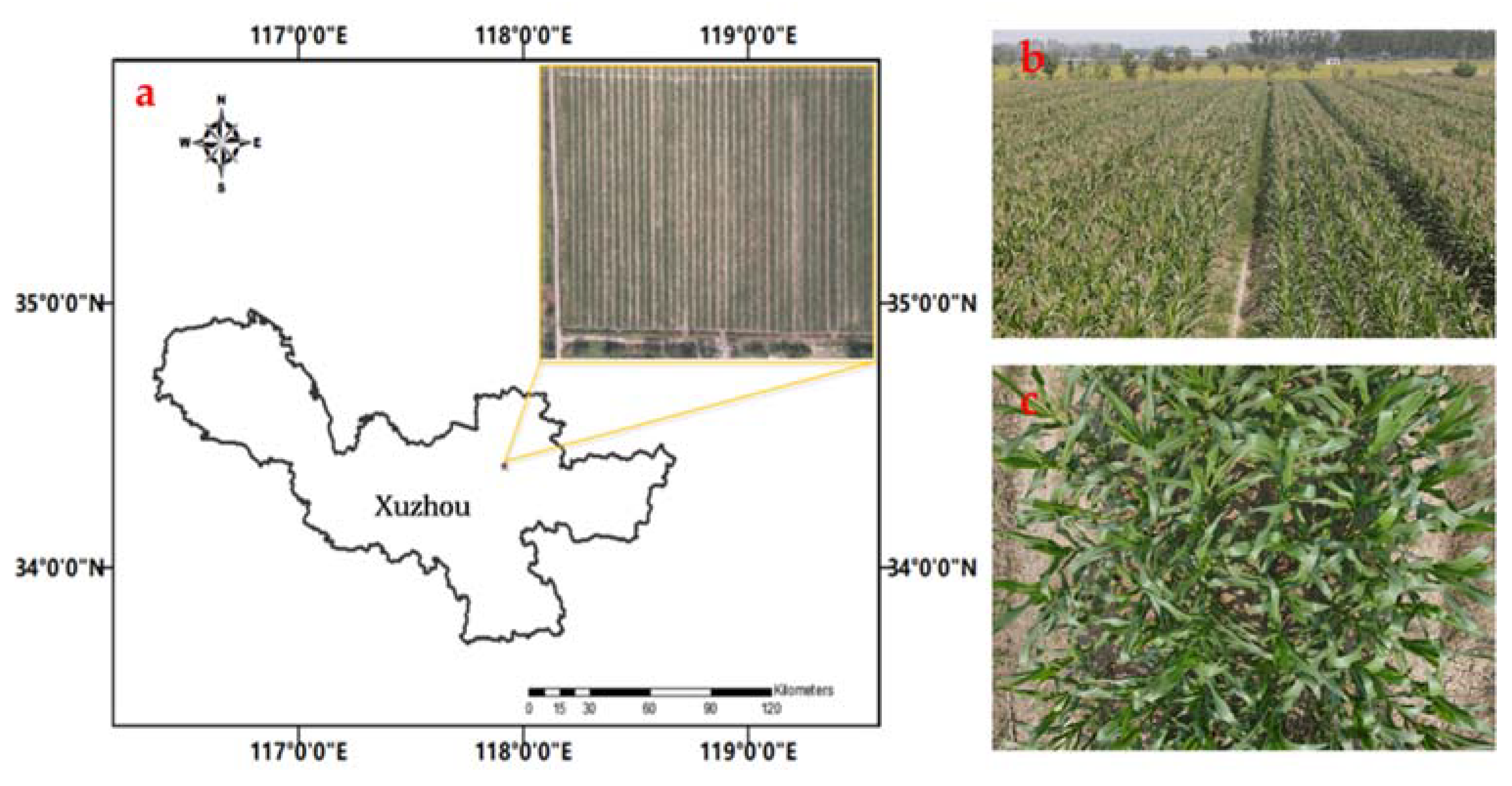
The data collection site was located in the fields around Tongshan County, Xuzhou City, Jiangsu Province, China, and the collection dates were 8, 19, and 24 September 2020. The experimental maize field covers an area of around five hectares (117.552616° E, 34.309942° N). According to a local plant protection station report, the growth stage of corn is filming between the jointing and heading stages when S. frugiperda invades and begins feeding. The field survey revealed that most of the S. frugiperda larvae were in the third and fourth instar. A few leaves with translucent windows also suggested the presence of first and second instar larvae. The number of maize plants that had completely lost growth capacity because of the decapitation caused by the feeding of S. frugiperda was in the single digits. Figure 1 shows the specific location and provides an aerial overview of the experimental field with an example sample image captured by the UAV.

A DJI Mavic Air2 UAV equipped with a 1/2-inch CMOS sensor with 12 million effective pixels was used to obtain the corn field images at a flight height of 1.5 m above the ground and a flight speed of 1.5 m/s. The reason for choosing a flight height of 1.5 m is that this was the lowest flight height for UAV for taking photos for maize in our study that would not be disturbed by the wind caused by the UAV. The ortho-photo images were acquired by flying and shooting alongside the rows of maize and two image sizes were available: 3000 × 4000 pixels and 6000 × 8000 pixels. The data captured have two characteristics: (1) different parcels of corn for the same date and (2) the same parcel for different dates; both of them guarantee the diversity of samples.

2.2. Image Annotation and Image Augmentation

Two sizes of image were acquired in this study: 3000 × 4000 pixels and 6000 × 8000 pixels. Images of 3000 × 4000 pixels require an excessive amount of graphic memory and down-sampling the original images would directly reduce the detail in the initial image. Therefore, a rectangular cross-division, i.e., even partition, was performed on the 8000 × 6000 pixels images in order to expand the amount of data while retaining the necessary information obtained in the original images. The sizes of the segmented images were finally unified at 3000 × 4000 pixels.

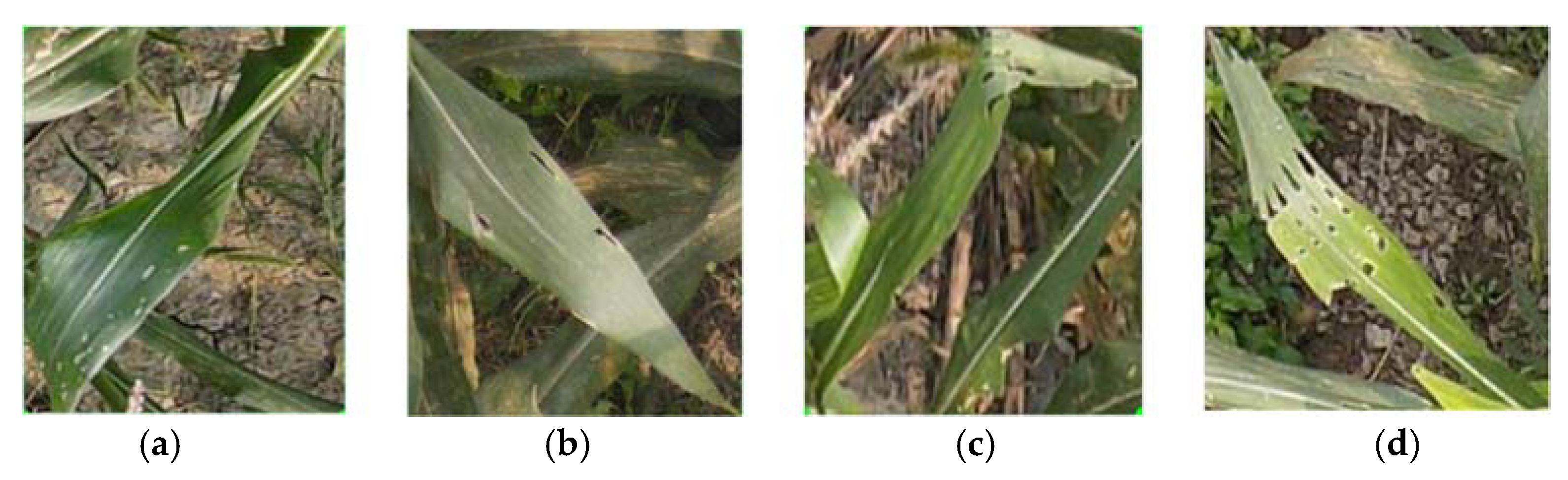
LabelMe, a commonly used open-source Python annotation toolbox, was used to produce an S. frugiperda object detection dataset based on the feeding habits and characteristics of S. frugiperda. Annotations were depicted in the forms of anchors. If there was more than one hole in a leaf appearing contiguously, rectangular was labeled covering all holes in the leaf. If there was one hole isolated in a leaf, the rectangular box wrapped the edge of the hole. The specific labeling criteria for the holes made by S. frugiperda feeding were as follows:

(1) Juvenile: leaves fed on by larvae before the third instar as evidenced by the presence of translucent film window-like holes in the leaves.

(2) Minor: leaves with minor feeding damage caused by larvae in the third instar or later, as evidenced by a small number of leaf holes. The proportion of hole area consumed by S. frugiperda is less than 10% in a unit area.

(3) Moderate: leaves with moderate feeding damage caused by the larvae of the third instar or later, as evidenced by a moderate amount of holes and successive holes in the leaves. The proportion of hole area consumed by S. frugiperda is between 10% and 30% in a unit area.

(4) Severe: leaves with severe feeding damage caused by the larvae of the third instar or later, as evidenced by numerous successive holes or missing leaf margins. The proportion of hole area consumed by S. frugiperda is higher than 30% in a unit area.

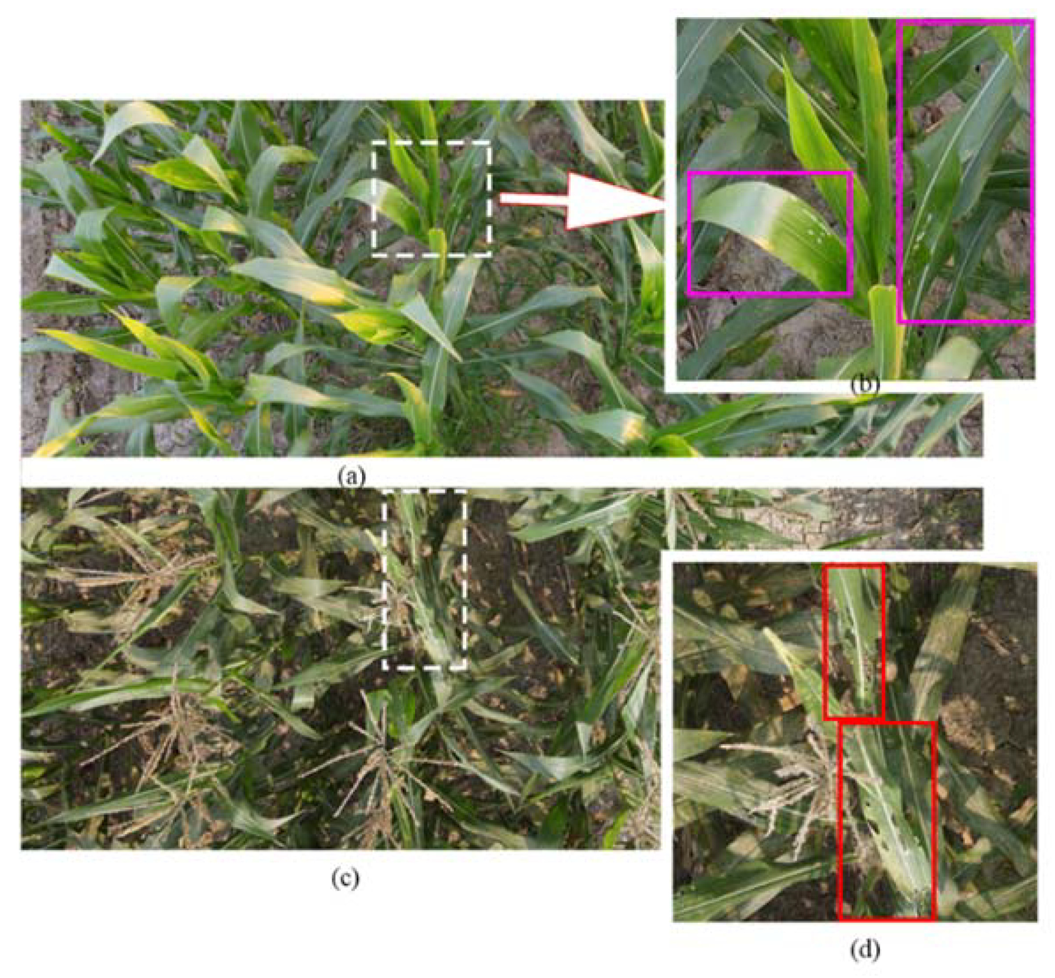
Annotated results for each category in the dataset are shown in Figure 2. Labeling was carried out by using rectangular boxes to cover the holes. Figure 3 shows an example of the labeled sample.

Due to the relatively small feeding area of maize S. frugiperda compared to the total image, after filtering out images without feeding zones, and ground truth anchor box and severity degree labeling, the maize S. frugiperda object detection dataset contained 585 images (3000 × 4000 pixels) with 3150 anchors showing feeding traces in total, i.e., 740 anchors showing evidence of juvenile feeding, 932 anchors showing minor damage, 954 anchors showing moderate damage, and 524 anchors displaying severe damage. The data distribution is shown in

Table 1. Initial feed severity of S. frugiperda anchor distribution.

Class	Amount	Criterion
Juvenile	740	Film window-like
Minor	932	<10%
Moderate	954	10–30%
Severe	524	>30%
Total	3150

.

The value in the criterion column was the proportion of hole area consumed by S. frugiperda in a unit area.

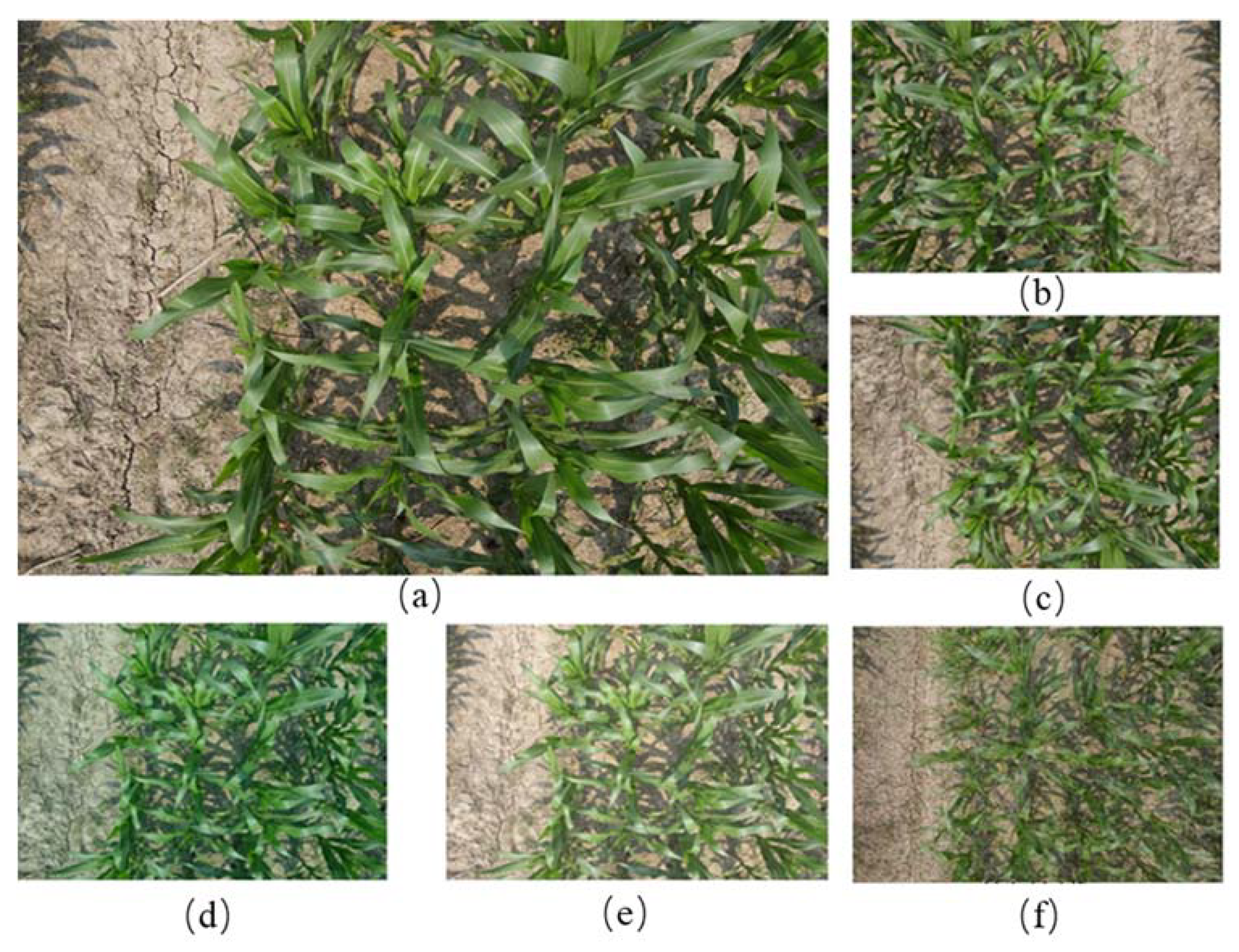
Therefore, data augmentations were used to enhance the original dataset in order to provide large amounts of training samples to better train the proposed Pest R-CNN model and make the model robust. Original images were transformed using random horizontal and vertical flips, random rotation, color transformation contrast transformation, and the mix-up strategy. Some of the transformation effects used are shown in Figure 4.

Finally, the maize S. frugiperda dataset was divided into a training subset and a validation subset at a ratio of 8:2. The training subset was used to train the Faster R-CNN model, and the validation subset was used for the final testing and evaluation of the object detection accuracy of the model.

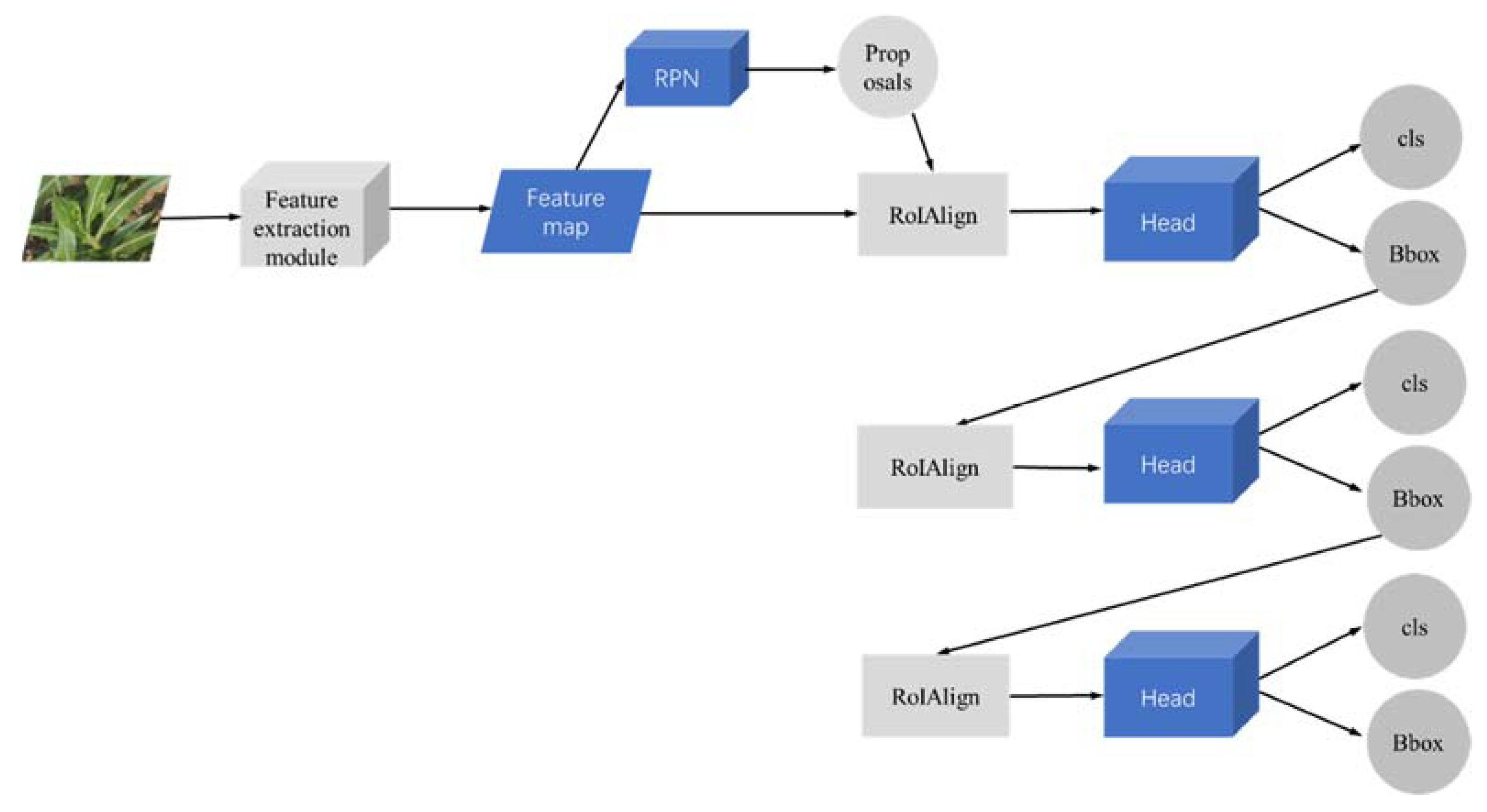
2.3. Model Architecture

An end-to-end deep learning object detection model named Pest R-CNN based on the classical object detection model Faster R-CNN was established to determine the location and feeding severity degree in images of maize S. frugiperda.

Figure 5 presents the overall structure of the S. frugiperda R-CNN detection model, Pest R-CNN.

The proposed model was divided into three parts in total, i.e., a feature extraction module, a region proposal network (RPN), and prediction parts. Feature extraction was used to generate rich spatial and contextual information for RPN object detection. The RPN was used to generate candidate anchors and the prediction parts were used to classify the S. frugiperda feeding severity degree and conduct more precise bounding box regression for anchor box.

2.3.1. Feature Extraction Module

Due to the differences between the spatial details included in the 8k and 4k images of the maize leaves and the different sizes of feed holes caused by S. frugiperda, the holes that were eaten by larvae younger than the third instar disappeared completely from the feature map, which resulted in non-detection after several convolutional operations. Cropping and scaling the images into different sizes before sending them to the detector would be expected to improve the accuracy; however, this would lead to a significant degradation in performance because of the need for repeated calculations. Aiming to improve the detection accuracy for specific S. frugiperda tasks, six points of improvement were proposed in Pest R-CNN compared with the original Faster R-CNN.

(1)

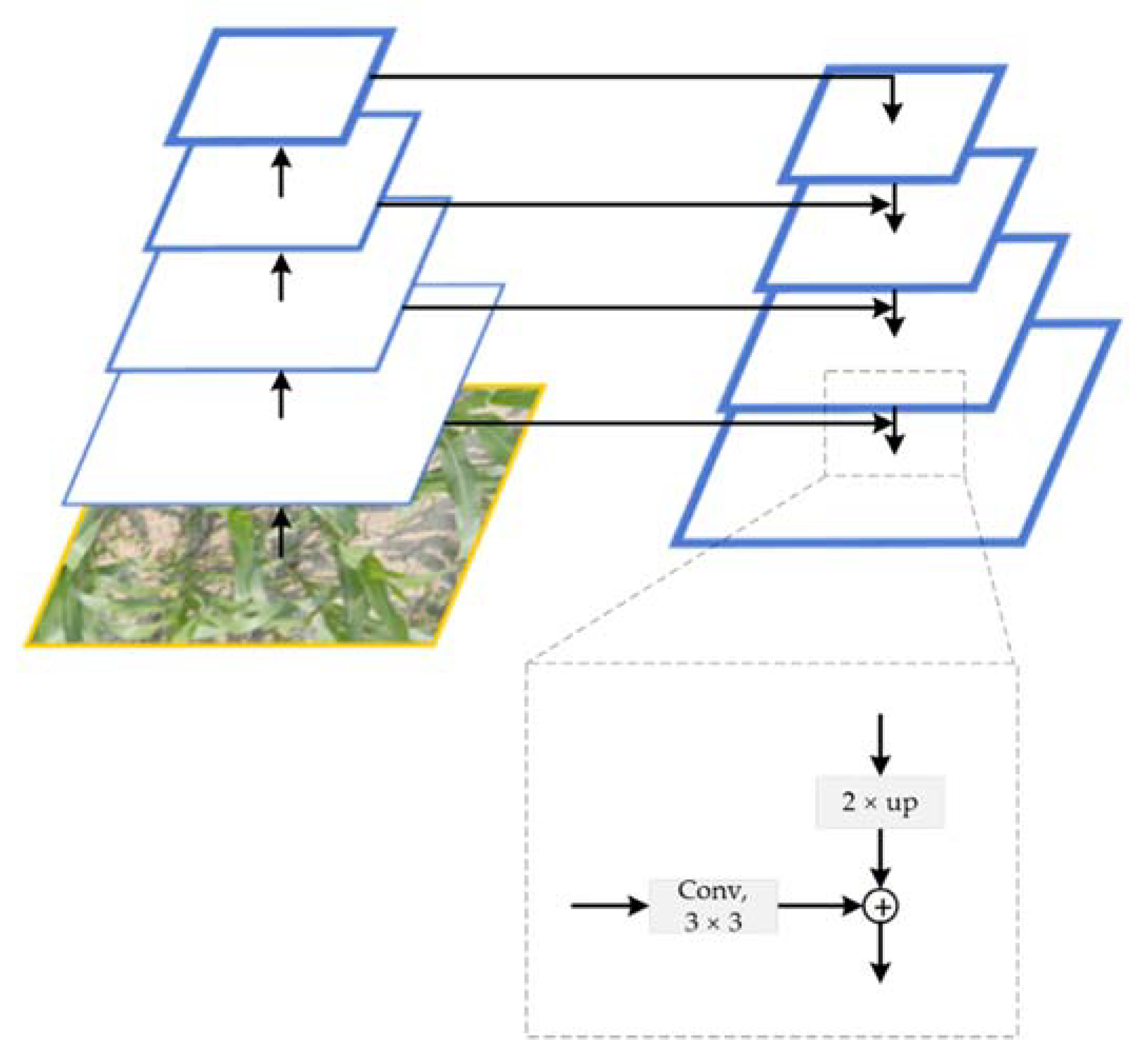
Feature pyramid network

Due to the stability performance of the ResNet network on various computer vision tasks such as classification, semantic segmentation, and object detection, considering the number of parameters of the network, ResNet-50 was selected as the backbone in the feature extraction module. However, in the original Faster R-CNN network, only the feature maps of the last layer of the extraction backbone, which did not contain enough context information for object detection, were used for further RPN modules. Therefore, in this study, the feature pyramid network (FPN) was added after the feature extraction backbone in the proposed Pest R-CNN.

Feature maps at four different scales were produced at four stages in the feature map pyramid from the bottom up, and the last layers of each stage were selected as feature maps. From top to bottom, a 1 × 1 convolution operation on feature maps of each stage was carried out using two-fold up-sampling. The processed layers were then cascaded with the feature map of the upper stage. The final feature maps were obtained through 3 × 3 convolution. The multi-scale detection of small holes in the maize leaves was beneficial for fusing low-level and high-level spatial and semantic contexts with only a minimal increase in the computational effort required. Figure 6 shows the FPN network diagram.

In order to further improve the performance of ResNet-50 in the feature extraction module, the 7 × 7 convolutional blocks were split into three 3 × 3 convolutional blocks, i.e., three convolutional blocks were performed in sequence, although doing so slightly increased the amount of computation required. Through this adaption, the receptive field was expanded from seven to eleven, adding more nonlinear structures, abstracting more in-depth features, increasing the depth of the network layer, and enhancing the capability for feature extraction.

(2)

Activation Function

The ReLU activation function was replaced by the Mish function so that the hard zero boundaries could be replaced with the smooth function. The activation function was used before batch-norming operations (BN operations), allowing the information to penetrate deeper into the neural network and achieve better accuracy and generalization.

(3)

Attention Mechanism

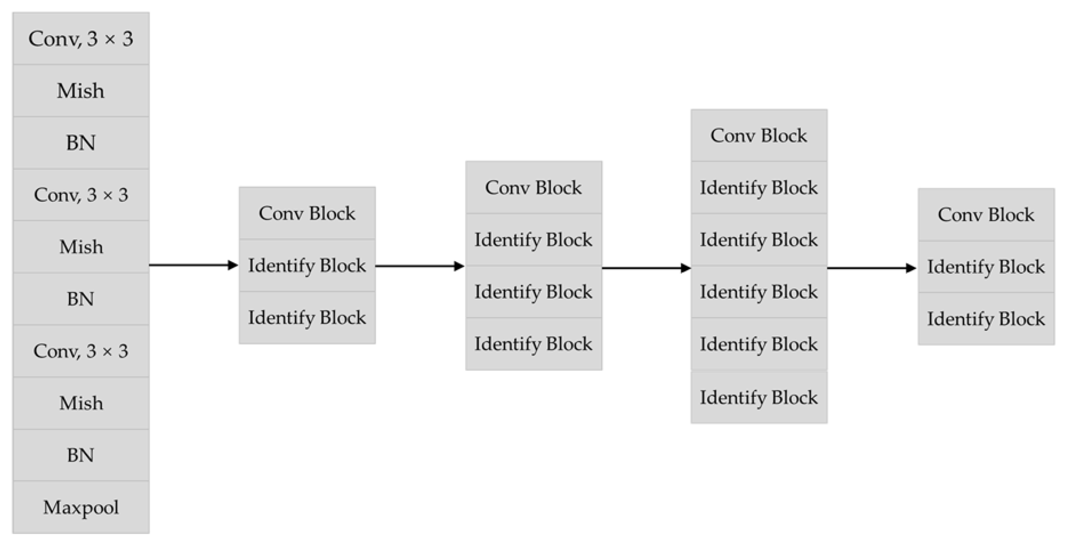
The overall structure of ResNet-50 is shown in Figure 7. In terms of the residual block used in the ResNet-50 structure, for the sake of capturing small differences in different degrees of severity in the proposed Pest R-CNN, the Conv Block and Identify Block in the original structure were adapted, i.e., the attention mechanism block was introduced to them.

Attention mechanisms were also integrated into the Conv Block and Identify Block, i.e., the channel attention module (CAM) and spatial attention module (SAM) were introduced to provide a higher weight for the feeding location of S. frugiperda and improved the detection capability by training the weight of the images with different features and in different regions.

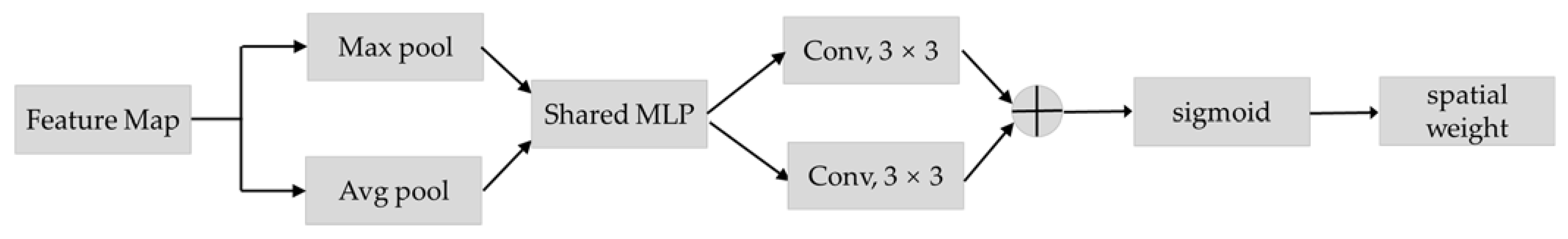
Due to the distinct feature extraction strength of maximum pooling and global semantic information extraction strength of average pooling, the SAM block combined maximum pooling and average pooling, i.e., feature maps were put into maximum pooling and average pooling branches separately, then the results of maximum pooling and average pooling were processed with a shared multi-layer perceptron and the sum of both branches were computed; the sigmoid function was finally used to form the pixel-wise weight, which was used to enhance the original features (Figure 8).

Channel-wise weights can be generated by a CAM block, specifically global maximum pooling and global average pooling. Then, the feature maps were concentrated and processed with a 3 × 3 convolution block and the sigmoid function restricted the value between 0 and 1 (Figure 9).

(4)

Group Convolution

The 3 × 3 convolution operation in the Conv block and Identify block residual blocks was replaced with group convolutions; specifically, the feature maps were evenly divided into four groups. Small residual blocks were added to the original residual unit structure to obtain 1 × 1, 3 × 3, 5 × 5, and 7 × 7 receptive fields gradually after splitting channels. Channel fusion was then performed to integrate more robust image features.

The difference between the Conv block and Identify block module was whether the 1 × 1 convolution in the upper branch was applied. The Conv block had the upper branch comprising of 1 × 1 convolution while the Identify block did not have 1 × 1 convolution in the upper branch. The specific structure is shown in Figure 10.

(5)

Deformation Convolution

The receptive field of ordinary convolution operations for the effective receptive field of each high-level feature map is a standard rectangle with a fixed geometric structure, which lacks an internal mechanism to handle geometric transformations. However, maize leaves are long and curved, with different postures and a high amount of geometric variation in the shape of the leaves. The contribution of all the pixel points in the receptive field to this point in the high-level feature map should therefore differ, and the size of contribution should match the shape of the maize leaves. Therefore, Pest R-CNN was fused with a deformable convolution used in DCN [34], and an offset was added that uses bilinear interpolation in conventional convolution.

In addition, the corresponding deformable ROI pooling was used for the pooling layer so that it could adaptively learn the receptive field and represent the different contributions of different pixels as a means of adapting to the geometric transformation of the maize leaves.

2.3.2. Region Proposal Network (RPN)

The size of the anchor box is vital for feature extraction in the corresponding zone and position of anchor box regression. The number of anchor boxes in the original Faster R-CNN network is nine, i.e., three scales (8, 16, and 32) and three ratios (1:2, 1:1, and 2:1). While the scale and ratio of the anchor box should be specifically determined according to the agricultural S. frugiperda detection task, obviously the initial three ratios cannot meet the demand of the task due to the varying ratio of width and height of corn leaves, so five ratios (1:4, 1:2, 1:1, 2:1, and 4:1) of the anchor boxes and three scales (4, 8, 16) were used in the proposed model based on the fact that a small area of the whole image was occupied by the leaf of the corn to improve the capacity of detecting small-scale objects, i.e., leaves feeding traces by S. frugiperda.

The region proposal network (RPN) network was applied in the candidate zone proposal stage to generate the anchors including objects. The specific implementation process of the RPN is shown in Figure 11. The feature maps generated by feature extraction module were input directly into the RPN to obtain the coordinates and confidence score of the generated anchors. As coordinates obtained in the RPN were in the original input image size scale, while the features maps processed with many convolution blocks were in a much smaller scale, it needs to transform the original size of the anchor into the range of the size of feature maps and resize to the same size for further prediction. In the original Faster R-CNN, this process was done with ROI Pooling module.

In our work, the ROI Pooling module was replaced with the ROI Align module with reference to Mask R-CNN in order to solve the problem of region mismatch in the two quantization processes [42]. The anchors generated went through the ROI Align module and were then processed with prediction heads to get the final class score, i.e., S. frugiperda feeding severity and the precise coordinates of the anchors.

2.3.3. Prediction Parts

As for the prediction parts, considering that in the training phase the real box position of the leaves consumed by S. frugiperda was annotated in advance, the suggestion box in the RPN with a real box intersection over union (IoU) greater than the threshold value of 0.5 can be identified as a positive result to participate in the subsequent bounding box regression learning. In the prediction stage, since the real box position of the infested leaves was unknown, all object boxes were treated as positive sample regression candidates, which led to poor quality of the object boxes in terms of prediction and “mismatch”. Simply increasing the IoU threshold to generate more accurate regression boxes and improving the detection accuracy was not suitable since that would produce overfitting problems and may cause more serious mismatch problems.

Therefore, a multi-layer structure was applied in the prediction heads of the proposed model, i.e., IoU values of 0.5, 0.6, and 0.7 were set as the thresholds for three linear layers for cascade training to avoid the possible mismatch problems mentioned above, as shown in Figure 5. Therefore, the detector in each layer focused on the object box according to the IoU value in a certain range, significantly improving the object detection accuracy.

2.4. Implementation Details

The Faster R-CNN model was implemented based on the PyTorch open-source deep learning framework and trained with an NVIDIA deep learning graphics processing unit (GPU) 2080.

To further improve the accuracy of the model and prevent the overfitting phenomenon, in this study, the model was trained using a cross-validation strategy and a multi-scale strategy based on augmented data. During the training process, a 5-fold cross-validation was used, i.e., the training set was randomly split into five subsets evenly, four were evenly used as training subsets and the remaining one was used as the validation subset. The cross-validation process was repeated five times to obtain five detection results. The average accuracy score of five cross-validations was used to reflect object detection accuracy.

As for the multi-scale training strategy, the size of the feature maps has a significant effect on the detection accuracy of the proposed detector. If the feature map generated in the feature extraction module is much smaller than the size of the original sample, e.g., 1000 × 1000 pixels, it will lead to a situation in which features describing the small holes cannot be easily captured by the detection network. If large feature maps were used, a larger load would be required to train the model. Therefore, a multi-scale training strategy was used, i.e., defining the sizes of several fixed feature maps in advance, and randomly selecting one size for training during each session. This training strategy can improve the recognition rate of small objects and improve the robustness of the detection model for leaves of different sizes.

The model was trained for 20 epochs. A momentum optimizer was adopted as the optimizer of the model and the momentum factor was set to 0.9. The initial learning rate was set to 0.02 and decayed in each epoch step.

The total loss comprised two main parts, i.e., an ROI and an RPN part, as illustrated in Figure 12 and calculated in Equation (1).

The loss of RPN and the loss of ROI were composed of the loss of classification and the loss of location, as shown in Equation (2) and Equation (3), respectively. In Equation (2), $L_{rpn\_cls}$ stands for the discrimination accuracy for the background and foreground and $L_{rpn\_loc}$ stands for the accuracy of the anchor position. In Equation (3), $L_{roi\_cls}$ and $L_{roi\_loc}$ stand for the accuracy of the severity degree of S. frugiperda and the accuracy of the ROI position, respectively.

The softmax loss function was used in all components of loss for the proposed model. In terms of the accuracy of classification, Equations (4) and (5) was used, where $N_{cls}$ stands for the quantity of samples; $p_i$ stands for the classification probability of Anchor $i$; $p_i^{*}$ stands for the possibility of ground truth, i.e., when Anchor $i$ is positive, the value of $p_i^{*}$ is 1 and when Anchor $i$ is negative, the value of $p_i^{*}$ is 0; and W is the regularization term. Equations (6)–(8) were used to calculate location accuracy, where $L_{reg}$ refers to the loss of regression of the coordinate parameter of anchor boxes, R adopts the SmoothL1 function, $t_i$ stands for coordinate parameters predicted by the proposed model, and $t_i^{*}$ refers to the true coordinate parameters of the ground truth anchor boxes.

$$L=L_{rpn}+L_{roi}$$

(1)

$L_{rpn}$ stands for the loss of RPN comprising $L_{rpn\_loc}$ and $L_{rpn\_cls}$.

$$L_{rpn}=L_{rp{n}_{cls}}+L_{rpn\_loc}$$

(2)

$$L_{roi}=L_{ro{i}_{cls}}+L_{roi\_loc}$$

(3)

$$L_{cls}=\frac{1}{N_{cls}}{\displaystyle \sum }_i{L}_{cls}\left(p_i,p_i^{*}\right)+W$$

(4)

$$L_{cls}\left(p_i,p_i^{*}\right)=-log\left[p_i{p}_i^{*}+\left(1-p_i\right)\left(1-p_i^{*}\right)\right]$$

(5)

$$L_{loc}=\lambda \frac{1}{N_{reg}}{\displaystyle \sum }_i{p}_i^{*}{L}_{reg}\left(t_i,t_i^{*}\right)+W$$

(6)

$$L_{reg}\left(t_i,t_i^{*}\right)=R\left(t_i-t_i^{*}\right)$$

(7)

$$Smoot{h}_{L1}\left(x\right)=\{\begin{array}{c}\left(0.5\ast {\sigma }^2\right)\ast x^2 \left|x\right|<1 \\ \left|x\right|-\left(0.5/{\sigma }^2\right) otherwise \end{array}$$

(8)

3. Results

The mean average precision (mAP) was used to evaluate the detection accuracy of the proposed model; it is the mean value of the AP values of all classes. AP is the actual metric for object detection and can be computed using the precision value (Equation (9)) and recall value (Equation (10)) through Equation (11). A true positive (TP) is a correctly predicted positive sample, a false positive (FP) is an incorrectly predicted negative sample, and a false negative (FN) is an incorrectly predicted positive sample. In Equation (11), $r$ refers to the recall value and ${\rho }_{interp}\left(r_{n+1}\right)$ means the max precision value in the different intervals of recall values.

$$\mathrm{precision}=\frac{TP}{TP+FP}$$

(9)

$$\mathrm{recall}=\frac{TP}{TP+FN}$$

(10)

$$\mathrm{AP}={\displaystyle \sum }_{r=0}^1\left(r_{n+1}-r_n\right){\rho }_{interp}\left(r_{n+1}\right)$$

(11)

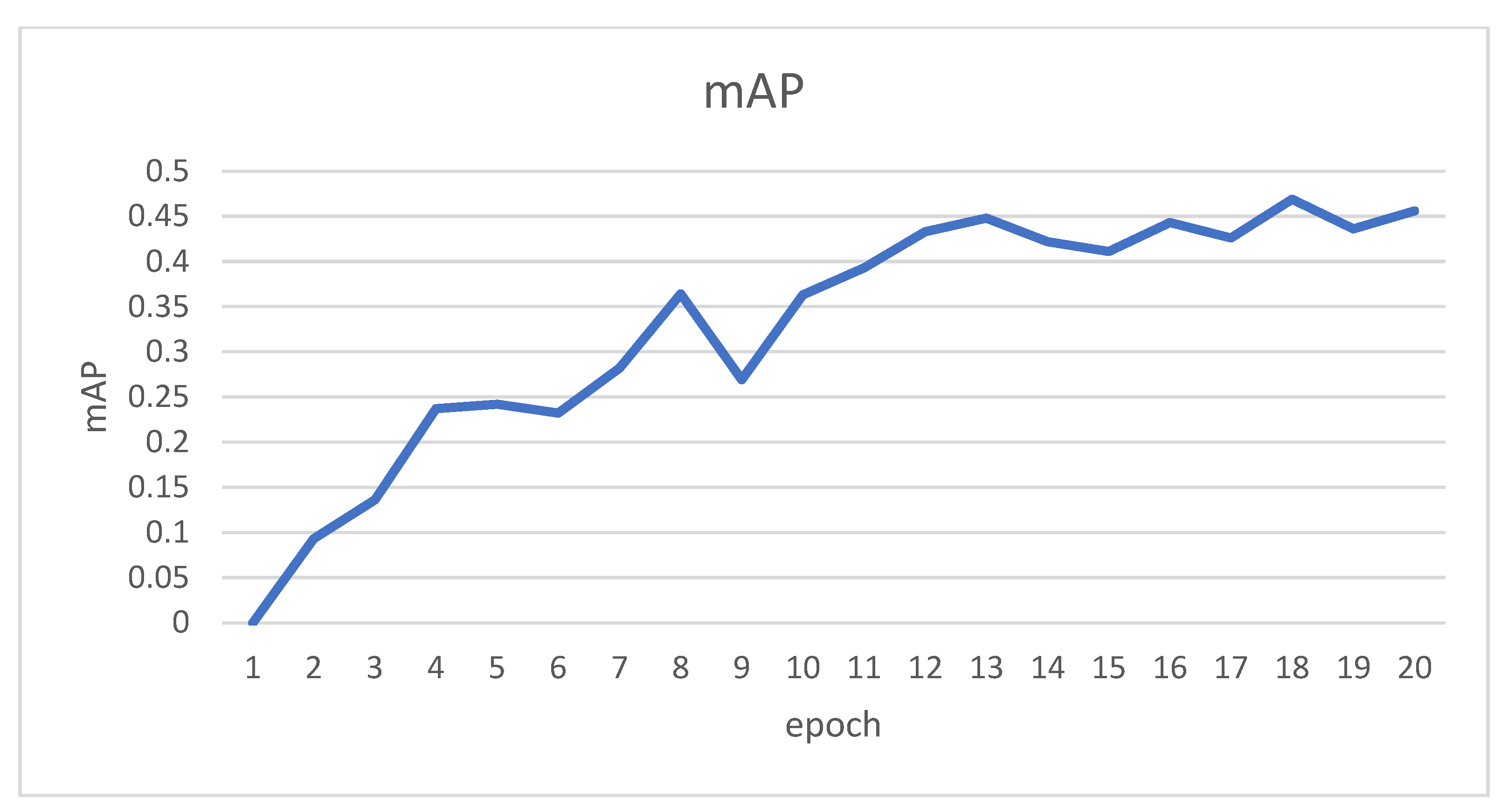
A mAP value of 43.6 was achieved by the proposed Pest R-CNN model, which is highly accurate. Figure 13 shows the change in the mAP during the process of training the Faster R-CNN model. It can be observed that mAP curves gradually lift and stabilize after the 14th epoch (Figure 13).

The mAP accuracy results for the five-fold cross-validation experiments were compared with the method of directly partitioning the dataset into 6:2:2 (training set, validation set, and test set, respectively). The specific implementation process of five-fold cross-validation was evenly partitioning the training dataset into five parts, using one part for validation and the other parts for training five times, and averaging the object detection accuracy of five separately trained Pest R-CNN models as the final accuracy.

The results shown in

Table 2. Comparison of the object detection accuracy for different data partition methods.

Data Partition Method	$\mathbf{m}\mathbf{A}\mathbf{P}$	$\mathbf{m}\mathbf{A}{\mathbf{P}}_{50}$	$\mathbf{m}\mathbf{A}{\mathbf{P}}_{75}$
5-fold CV	43.6	60.2	46.3
Hold-out	40.2	57.3	42.6

Five-fold CV stands for 5-fold cross-validation; hold-out stands for not adopting a validation subset; a whole training set was used to train the model. Numbers in bold represent the highest accuracy in terms of mAP, mAP₅₀, and mAP_75.

indicate that the use of cross-validation in the Faster R-CNN model effectively reduced the noise and achieved a better accuracy of object detection of S. frugiperda.

After training the Faster R-CNN model, a mAP of 43.6 was achieved in the test dataset, showing the practicability and versatility of the proposed Pest R-CNN model in detecting S. frugiperda in maize. In the case of the same data augmentation method, the same data partition method for the maize S. frugiperda dataset and training with the original Faster R-CNN model yielded mAPs of 31.3 for the validation set and 22.5 for the test set.

We compared our proposed model with Faster R-CNN and the latest object detection model, i.e., YOLO v5, and the dataset was divided according to the previous experiment in the ratio of 8:2; according to the limitation of the capacity of the GPU, the size of the trained and validation images was cropped into 2000 × 1500 pixels. The object detection accuracy comparison is listed in

Table 3. Comparison of the object detection accuracy for different object detection methods.

Method	mAP	mAP50
Faster R-CNN	22.5	31.2
YOLOv5	12.1	24.6
Pest R-CNN	40.2	57.3

All experiments were conducted with hold-out data partition method.

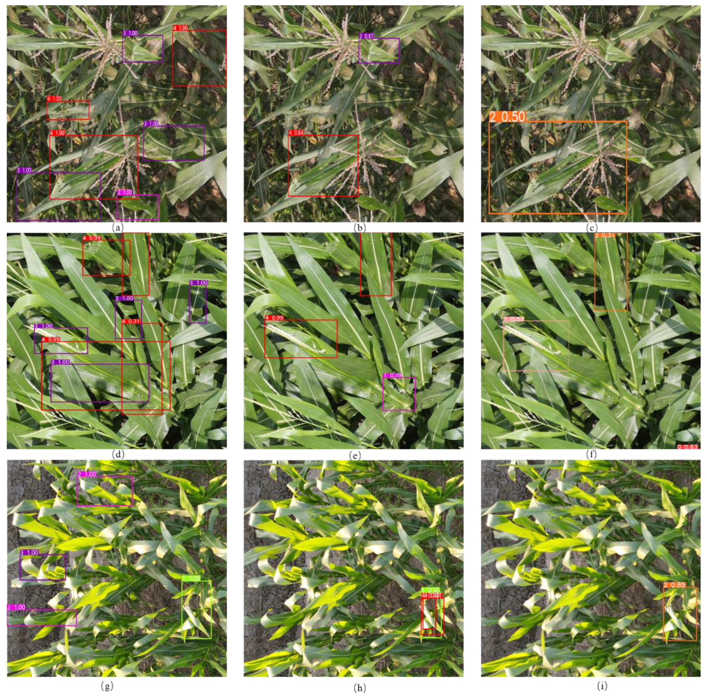
. Figure 14 shows the intuitive comparative view of the object detection results of the proposed Pest R-CNN model, original Faster R-CNN, and YOLOv5.

Faster R-CNN is a classical model that is generally used for object detection. However, it is mainly oriented to daily common scenarios and is not well adapted to the field of agricultural diseases and pests. In particular, because the images used in this study have a high spatial resolution with large amounts of information, the original structure cannot accurately predict the presence of the features associated with pests feeding. The FPN structure, deformable convolution, multi-scale strategy, etc., were adopted on the basis of the original model to improve object detection accuracy. Figure 14 shows the superiority of the proposed model compared with the original Faster R-CNN model and YOLOv5. It can clearly be seen that the amount of anchor boxes generated by the proposed Pest R-CNN is much larger than that of the original Faster R-CNN. In terms of detected anchor boxes, the predicted results of Pest R-CNN are more concentrated on the feed area of S. frugiperda. The classification accuracy of feeding severity degree of the proposed model was also higher than Faster R-CNN and YOLOv5 by a large margin. Both aspects confirmed that a high accuracy of object detection can be achieved in the proposed model intuitively.

4. Discussion

Three aspects of the proposed model will be discussed in this section through the ablation studies, i.e., the effects of the model modules, the effects of augmentation methods, and the effects of regularization methods. We hope this will be beneficial to the design of a network architecture. Further improvements to the agricultural pest object detection model are also pointed out in this section. Details will be described in the following parts.

4.1. Ablation Experiment on the Adapataion Module of the Pest R-CNN

Table 4. The object detection accuracy comparison of the ablation studies.

Model Architecture/Accuracy	mAP	$\mathbf{m}\mathbf{A}{\mathbf{P}}_{50}$	$\mathbf{m}\mathbf{A}{\mathbf{P}}_{75}$
Faster R-CNN	22.5	31.2	26.8
ResNet50-FPN	30.7	42.5	32.2
ResNet50-A-FPN	35.8	49.3	38.3
ResNet50-A-G-FPN	37.5	47.2	39.1
ResNet50-A-G-FPN-DCN	38.5	53.3	40.2
Pest R-CNN(ResNet50-A-G-FPN-DCN-MS)	43.6	60.2	46.3

Faster R-CNN means the original model, ResNet50-FPN, stands for adopting ResNet50 as the feature extraction backbone, and FPN was used to aggregate multi-scale features. A, G, DCN, and MS stand for the channel and spatial attention mechanism, group convolution, deformable convolution, and multi-scale training strategy, respectively. The bold values are the highest values achieved by the models.

shows the improvement in detection accuracy introduced by the adaption module. From Table 4, only adding the FPN structure increased the mAP75 value by 5.4 compared with the original Faster R-CNN model, which proved the effectiveness of the FPN. The reason for that is the multi-scale feature extraction ability inherited in the FPN. The AP75 was further improved when group convolution operations were used in the residual block in the ResNet-50 backbone. Since cascade convolution operations were applied in the grouped channels of features, the residual block had a better feature extraction ability. DCN further improved the accuracy, and a possible reason for this is that deformable convolution has the capacity to capture irregular zones suitable for feeding zone recognition. Moreover, when the multi-scale training strategy was used, the mAP value was further increased due to the improvement in model robustness.

The FPN structure improved the detection performance the most, showing the importance of different level feature aggregation in the area of small object detection in agriculture. We believe that the detailed ablation studies could be beneficial for designing more advanced agricultural object detection models.

4.2. Comparison of the Object Detection Accuracy of Different Data Augmentation Methods

With the same experimental setting, the effect of different methods of image augmentation has been compared.

Table 5. The mAP values of different augmentation methods.

Experiment/Accuracy	mAP	mAP50	mAP75
All	43.6	60.2	46.3
Without G-transformation	39.7	56.6	45.3
Without C-transformation	35.5	52	39.9
Without mix-up	41.4	57.9	42.8

“All” refers to the use of geometric transformation, color transformation, and the mix-up strategy augmentation method; “without G-transformation” refers to without geometric transformation; “without C-transformation” refers to without color transformation. Bold represents the highest accuracy and italics represent the lowest values in terms of mAP, mAP50, and mAP75.

shows the object detection accuracy in terms of mAP, mAP50, and mAP75. As shown in Table 3, the accuracies of all ablation studies are lower than the original methods, proving that it is vital to conduct image augmentation to improve the performance of the proposed model.

Without color transformation augmentation, the accuracy mostly decreased compared with other ablation studies. The possible reason for this phenomenon is that color space is the most intuitive feature; color transformation can generate more features, so the performances of the proposed models have been greatly improved. Without geometric transformation, the accuracy decreased the least, mainly because the geometric transformations used in this study were random horizontal flips, vertical flips, and rotations, which are simple to carry out, while the augmentation forms are limited. With the mix-up strategy, newly generated samples contained some unavoidable noise, possibly due to the complex agricultural production background environment, which may restrict the actual effect of the mix-up strategy.

4.3. Comparison of Accuracy of Different Regularization Methods

In order to avoid overfitting, the total loss function in the proposed model contains a regularization term. Comparison studies based on using different regularization methods were conducted to provide insights for choosing appropriate regularization methods in further studies. In order to measure the object detection performances between the training subset and test subset, the training subset was divided according to the ratio of 3:1 randomly, where the first part was considered as the training subset and the other part was considered as the validation subset.

Table 6. Comparison of different regularization methods.

Regularization Method	V_mAP	T_mAP
L2	45.3	43.6
L1	47.1	40.2
None	44.9	33.8

V_mAP and T_mAP stand for the mAP values of the proposed model on the validation dataset and test dataset, respectively.

shows the detection of the model performance on validation and test subset accuracies. From Table 6, it can be observed that if no regularization method was used, a large performance gap in mAP exists between the validation subset and test subset, showing overfitting problems and the effectiveness of the augmentation methods. Although the highest mAP value was achieved by L1 regularization, the performance of L2 regularization is better than that of L1 regularization, i.e., the difference between the validation and test dataset mAP values is 1.7% compared with 6.9%, showing a better generalization ability and lower degree of overfitting and verifying the effectiveness of the L2 regularization method.

4.4. Discussion about Cost and Further Improvement Aspects

As for the cost for the actual application of this proposed model, the high-spatial-resolution data were collected by a DJI Mavic Air2, whose price is around CNY 5000, which is acceptable for precise plant protection. In further studies, it is expected that pest object detection will be more closely combined with the use of UAVs.

The data for this experiment were mainly collected at a flight height of 1.5 m above the ground. In follow-up studies, the relationship between the spatial resolution of images and the object detection accuracy of the proposed models could be further analyzed in order to obtain an optimal spatial solution, i.e., flight height to meet the demand for rapid image acquisition and accurate object detection accuracy over an entire region. Similarly, the angle of data acquisition requires further investigation. In this experiment, all images were collected at a 90° ortho-angle; the main body of the upper leaves of maize was almost horizontal, and S. frugiperda prefers to feed on the uppermost young leaves. However, this will lead to an absence of imagery of the second upper layer of leaves likely consumed by S. frugiperda before the uppermost grew; to some extent, this is not conducive to understanding the overall situation of S. frugiperda infestation. Therefore, in future studies, data of S. frugiperda invasion leaves should be collected from multiple angles for comparison in order to obtain the optimal image capture angle for S. frugiperda infestation detection.

5. Conclusions

A novel Pest R-CNN based on the Faster R-CNN was proposed for maize S. frugiperda feed-trace object detection, combining an FPN, attention mechanism, deformable convolution, and multi-scale strategy. The model was trained and validated with data collected in a real-world agriculture scene and labeled according to plant protection knowledge. The mAP values of the Pest R-CNN were higher than the original Faster R-CNN by a large margin, showing the effectiveness of the proposed model. To the best of our knowledge, this is the first attempt to apply object detection using a deep learning methodology in S. frugiperda feed traces. The model can be used for fast severity degree surveying on a large scale. This proposed model also proved the potential of deep learning by combining it with low-cost remote-sensing methods and applying them in actual agricultural pest detection. Ablation studies with respect to adapted modules, image augmentation methods, and regularization methods could provide information about the network architecture design and improve the robustness of agricultural pest objection detection. For future studies and further improvement of the transferability and generalization of the proposed model, more images of leaves infested by pests in different geography zones and more images of leaves infested by different types of pests could be collected to build a pest object detection model for multiple types pests. In addition, due to the ability of the abundant features of multi-spectral and hyper-spectral images, these data could be involved in further studies of deep learning pest object detection.