
Effects of Aeroelastic Walls on the Aeroacoustics in Transonic Cavity Flow †

1
Division of Fluid Dynamics, Department of Mechanics and Maritime Sciences, Chalmers University of Technology, 41296 Gothenburg, Sweden
2
SAAB AB, Aeronautics, 581 88 Linköping, Sweden
*
Author to whom correspondence should be addressed.
†
This paper is an extended version of our paper published in the 19th International Forum on Aeroelasticity and Structural Dynamics (IFASD), Madrid, Spain, 13–17 June 2022; Paper No. IFASD-2022-020.
Aerospace 2022, 9(11), 716; https://doi.org/10.3390/aerospace9110716
Submission received: 15 September 2022
/
Revised: 7 November 2022
/
Accepted: 8 November 2022
/
Published: 14 November 2022
(This article belongs to the Special Issue Aeroacoustics and Noise Mitigation)
Abstract
:The effects of elastic cavity walls on noise generation at transonic speed are investigated for the generic M219 cavity. The flow is simulated with the Spalart–Allmaras (SA) improved delayed detached-eddy simulation (IDDES) turbulence model in combination with a wall function. The structural analysis software uses a modal formulation. The first 50 structural normal mode shapes are included in the simulation, spanning frequencies of 468–2280 Hz. Results are compared with those from a reference simulation with rigid cavity walls. A spectral analysis of pressure fluctuations from a microphone array above the cavity evinces a distinct tone at 816 Hz, which is absent in the reference simulation. Furthermore, the power of the 4th Rossiter mode at 852 Hz is depleted, implying a significant energy transfer from the fluid to the structure. Spectral proper orthogonal decomposition (SPOD) is employed for analyses of cavity wall pressure fluctuations and wall displacements. The SPOD mode energy spectra show results consistent with the spectra of the microphone array with respect to the tone at 816 Hz and the depletion of the energy at the 4th Rossiter mode. Furthermore, the SPOD mode energy spectra show energy spikes at additional frequencies, which coincide with structural eigenfrequencies.
1. Introduction
Cavity flows are present in several aerospace applications. For instance, weapon bays, landing gear bays, and other openings in an airframe. Cavity flows are inherently unsteady and characterised by energetic tonal and/or broadband pressure fluctuations. Broadband noise predominates in shallow cavities, whereas tonal components predominate in deep cavities [1]; the tonal components are referred to as Rossiter modes. The presence of energetic pressure fluctuations has several potential implications; it may affect the aerodynamics, structural integrity, interior noise level, and the surroundings in the form of noise. Vibrations stimulated by dynamic loads may be detrimental to the structure and provoke structural instabilities and failures. For instance, protracted vibrations may cause acoustic fatigue. Furthermore, vibrations can propagate in the structure and apparatuses may be exposed to vibration levels beyond their certified limit.
High Reynolds number cavity flows have been extensively investigated, both theoretically and experimentally, and from a variety of perspectives. A multitude of numerical studies on cavity flows using computational fluid dynamics (CFD) with a host of different turbulence modelling techniques have been reported in the literature. The use of unsteady Reynolds-averaged Navier–Stokes (RANS) for cavity flows is reportedly less accurate [2,3]; by its nature, unsteady RANS cannot predict the full spectrum of turbulent scales [3]. Large-eddy simulation (LES) provides excellent results [4], and many hybrid RANS-LES methods show good agreement with experimental data [2,5,6]. However, cavity flows at high Reynolds numbers are challenging [3]; a variety in accuracy has been reported regarding the prediction of Rossiter mode frequencies and magnitudes with the use of hybrid RANS-LES techniques.
Many studies focusing on cavity flow noise generation have been reported in the literature. Turbulence-resolving methods are integral to the prediction of noise stemming from cavity flows [7]. Hybrid RANS-LES methods have successfully been used in many studies. There are a mere few studies presented in the open literature on the conjunction of aeroelasticity and aeroacoustics, notwithstanding the array of publications on cavity flow noise generation. A recent study by Łojek et al. [8] investigated the effect of elastic cavity walls on noise generation at a very low Reynolds number. They used the detached-eddy simulation model for flow simulation and the Ffowcs Williams and Hawkings acoustic analogy to predict far-field noise. They reported that the elastic cavity generates tonal noise in the range of 1–10 kHz, at frequencies that coincide with structural eigenfrequencies. Several of the tones have a sound pressure level (SPL) that is approximately 30 dB higher than the broadband noise in the corresponding rigid cavity.
We examine the effects of elastic cavity walls on the noise generation at transonic speed. The M219 cavity is used, the cavity is simulated with both rigid and elastic cavity walls. A flow solver validation is undertaken with the rigid cavity. Experimental data by Henshaw [9] and LES data by Lerchevêque et al. [4] are used for reference. No experimental reference data are available for the elastic cavity simulation, and the elastic structural model is fictitious. A microphone array is situated above the rigid and the elastic cavity. The effects of the elastic walls are evaluated by spectral analysis of the microphone signals. Furthermore, spectral proper orthogonal decomposition (SPOD) is employed to analyse wall pressure fluctuations for the rigid and the elastic cavity. Additionally, the SPOD of the wall displacements are presented for the elastic cavity. The flow solver validation is undertaken with the wind tunnel configuration used by Henshaw [9]. A simplified geometrical setup is used to evaluate the effects of the elastic cavity walls. The effects of the rigid simplified geometrical configuration in relation to the rigid wind tunnel configuration are presented as well.
The accumulative experience of hybrid RANS-LES methods in combination with wall functions is not vast. However, the practical interest is high, particularly for industrial aeroelastic applications at high Reynolds numbers where resolved turbulence and grid deformations are of importance. A few benchmark cases have been reported in the literature [10,11], with propitious results. This paper does not provide an exhaustive examination of hybrid RANS-LES methods in combination with wall functions. The methods employed are merely evaluated in terms of the SPL and the overall sound pressure level (OASPL) derived from cavity wall pressures, and velocity and shear stress profiles are compared with LES data [4].
The forthcoming section describes the numerical methods. The following section introduces the two geometries and the corresponding computational grids as well as results from simulations on the rigid cavity. The ensuing section introduces the finite element (FE) model and its modal representation. Subsequently, the results from the fluid–structure interaction (FSI) simulation are presented and compared to the reference simulation of the rigid cavity in order to evaluate the effects on the noise generation due to the elastic walls. The closing section summarises the paper and the most important findings.
2. Numerical Methods
The software M-Edge [12,13] is used for the flow simulations and the FSI simulation. M-Edge incorporates a Navier–Stokes flow solver and a modal-based solver for structural analysis.
2.1. Method for Flow Simulation
The compressible flow solver M-Edge uses an edge-based formulation and a node-centred finite-volume method to discretise the governing equations. A second-order central difference scheme with a Jameson-type scalar artificial dissipation is employed for the spatial discretisation of the momentum equation and for the turbulent transport equations. The equations are integrated in time using an implicit second-order backward differencing scheme together with a dual time-stepping methodology, which uses an explicit steady-state time marching scheme [12,13]. Here, fifty sub-iterations are performed for each time step for all simulations, which results in an average decrement of the order of the maximum error of the density residual. The aerodynamic coefficients and the maximum temperature are converged within the 50 sub-iterations. The delayed detached-eddy simulation (DDES) [14] based on the Spalart–Allmaras (SA) model [15] and SA-based improved DDES (IDDES) [16] turbulence models are employed. The free-stream flow properties correspond to the conditions used in the wind tunnel test [9]; the conditions are presented in Table 1. A total physical time of s is simulated for all cases. The first s is discarded to ensure that the flow field is established for the analysed signals; hence, the latter s is used for statistical analysis.
Rossiter mode powers and frequencies are generally not constant over time. The mode power, in particular, could change substantially through so-called mode switching [17], which means that the mode energy can switch from one mode to another over large time scales [18]. This makes it more complicated to ascertain a statistically stationary flow field. Here, mean values, root mean square values, and Rossiter frequencies based on cavity wall pressure fluctuations are monitored to confirm that the flow field is established.
A time step of s is used, which is 0.6 percent of the cavity length travel time. The CFL number, , where U is the velocity magnitude and is the cell length in the direction of the velocity, is approximately unity or less inside the cavity and at most locations outside the cavity. However, the use of a structured grid—see Section 3.1 and Section 3.2—entails that streaks of wall-resolved cells reach the free stream above the cavity front and rear walls. The CFL number in the streaks above the boundary layer is approximately 10. This is also the main incentive to employ a wall function in this study. The wall function allows for a much larger first cell height, which in turn enables the use of a larger time step.

Table 1.
Free-stream conditions.
| Mach Number | Speed, | Static Pressure | Static Temperature |
|---|---|---|---|
| 0.85 | 278.16 m·s | 62,100.00 Pa | 266.53 K |
2.2. Method for Structural Simulation
The modal-based FSI formulation in M-Edge is strongly coupled to the flow solver, in the sense that the flow solver and the structural solver exchange information in each sub-iteration. The method is based on the eigenvalue problem of the full structural FE model and provides a set of linear equations describing structural deformations. A Newmark time-integration scheme is used. Validations of the modal-based solver have previously been undertaken for FSI problems [19,20]. The FE model and its modal representation are introduced in Section 4.
3. Simulations with Rigid Cavity Models
This section introduces the cavity geometry, the two computational domains, and the corresponding grids. The wind tunnel model that is used for the flow solver validation is first presented, followed by the simplified geometry, which is used for the ensuing FSI simulation. The wind tunnel model serves as a benchmark case for the choice of turbulence model for the FSI simulation. Simulation results are compared with experimental data for the wind tunnel model and with LES data. Furthermore, a comparison between the wind tunnel configuration and the simplified configuration is presented.
3.1. Wind Tunnel Model
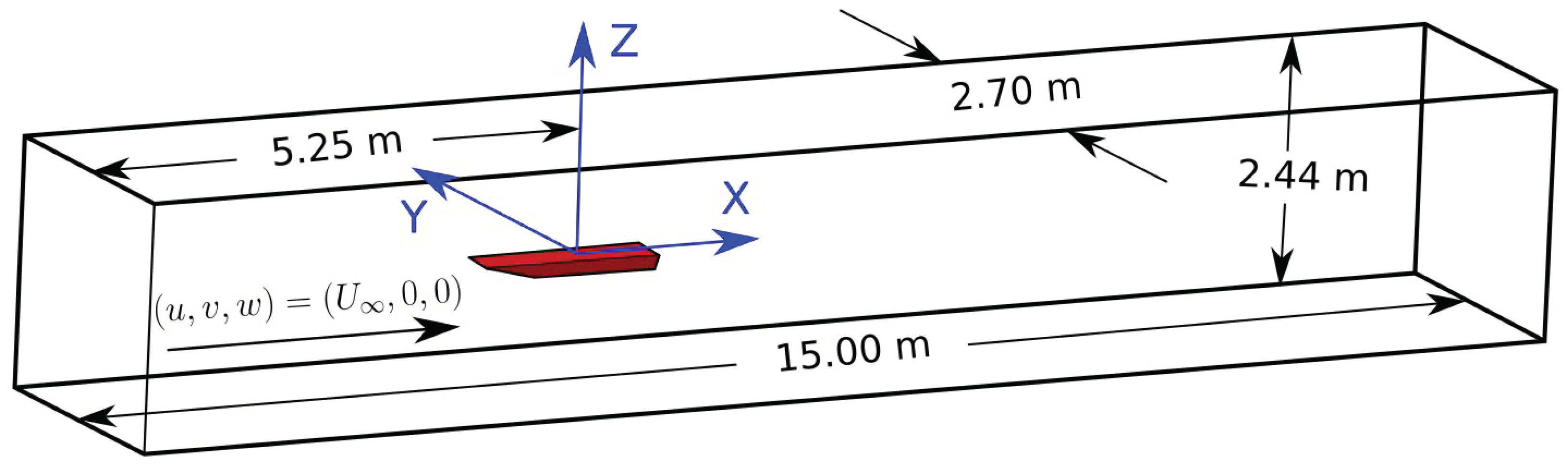
The computational grid used for the validation of the flow solver corresponds to the geometry of the wind tunnel experiment by Henshaw [9]. The dimensions of the wind tunnel test rig are shown in Figure 1. The size of the computational domain corresponds to the size of the wind tunnel test section, which is shown in Figure 2. The sting used to fasten the rig in the wind tunnel is not included in the CFD model. The main reason for excluding the sting is to facilitate the grid generation and to make the grid as simple as possible. Potential influences on the flow in the cavity from the sting are considered negligible.
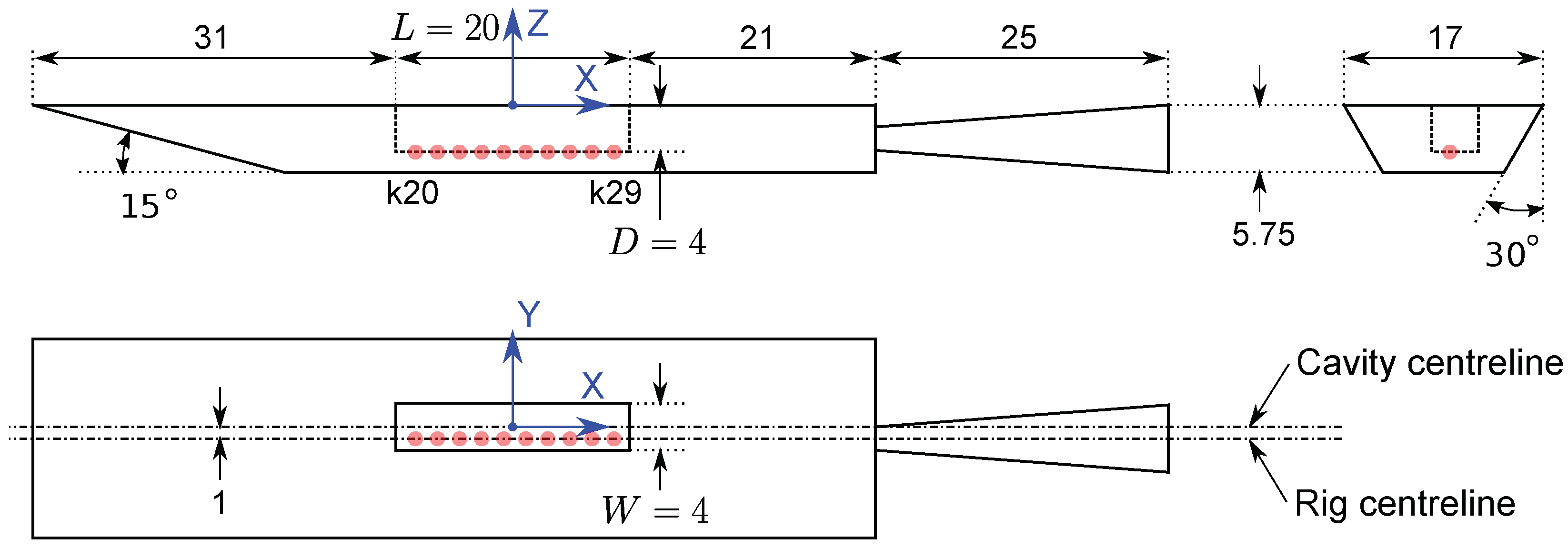
Figure 1.
Schematics of the M219 cavity used in the wind tunnel experiment. Length units in inches. Positions for the Kulite transducers are indicated by red markers. L, W, and D are the cavity length, width, and depth, respectively.
Figure 1.
Schematics of the M219 cavity used in the wind tunnel experiment. Length units in inches. Positions for the Kulite transducers are indicated by red markers. L, W, and D are the cavity length, width, and depth, respectively.

Figure 2.
Computational domain for the wind tunnel model.

The positions of the Kulite transducers used for measurements in the wind tunnel test are shown in Figure 1 and listed in Table 2. The positions of the transducers are defined in the coordinate system according to Figure 1, with the origin in the cavity centre and on the plane of the rig’s top surface. The original geometry was defined in imperial units; thus, it is convenient to restate the dimensions and the positions of the Kulite transducers here in imperial units. For clarity, all other dimensions and quantities are given in metric units.
Table 2.
Location of the Kulite transducers.
| Probe | x (inch) | y (inch) | z (inch) |
|---|---|---|---|
| K20 | −9.0 | −1.0 | −4.0 |
| K21 | −7.0 | −1.0 | −4.0 |
| K22 | −5.0 | −1.0 | −4.0 |
| K23 | −3.0 | −1.0 | −4.0 |
| K24 | −1.0 | −1.0 | −4.0 |
| K25 | 1.0 | −1.0 | −4.0 |
| K26 | 3.0 | −1.0 | −4.0 |
| K27 | 5.0 | −1.0 | −4.0 |
| K28 | 7.0 | −1.0 | −4.0 |
| K29 | 9.0 | −1.0 | −4.0 |
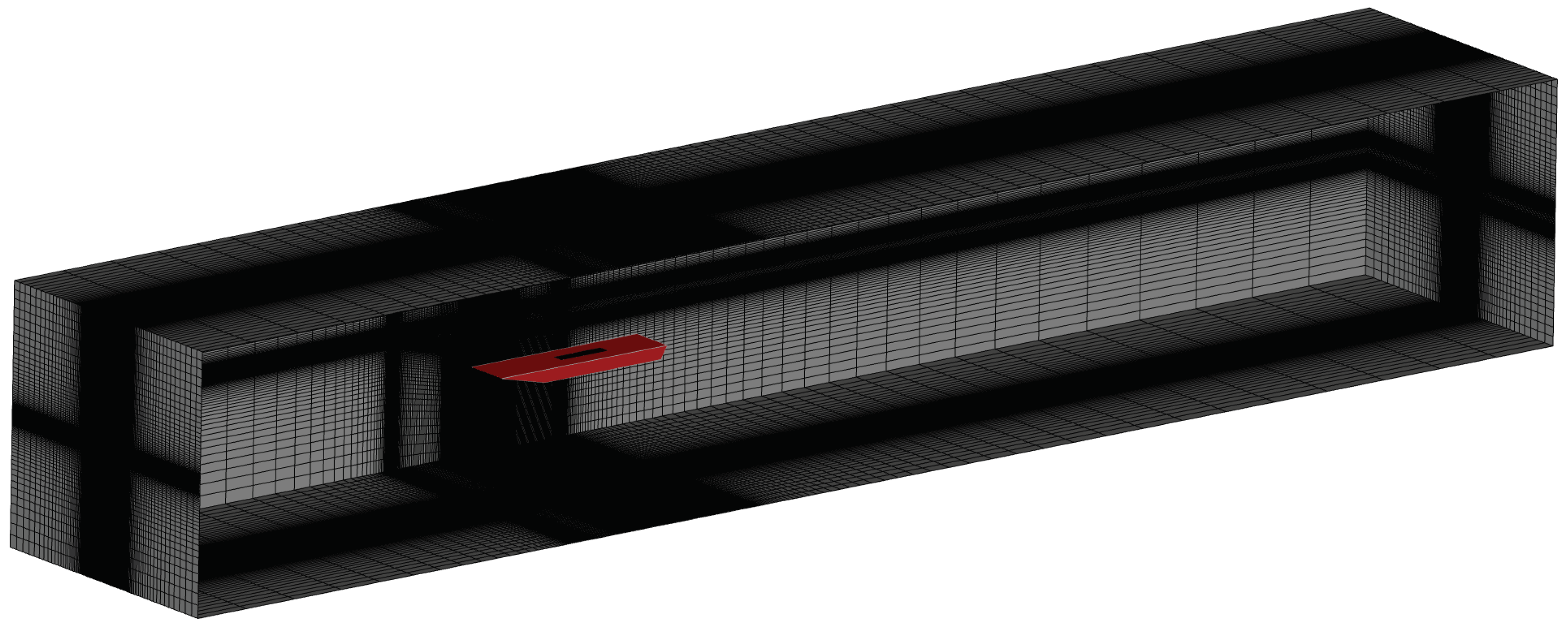
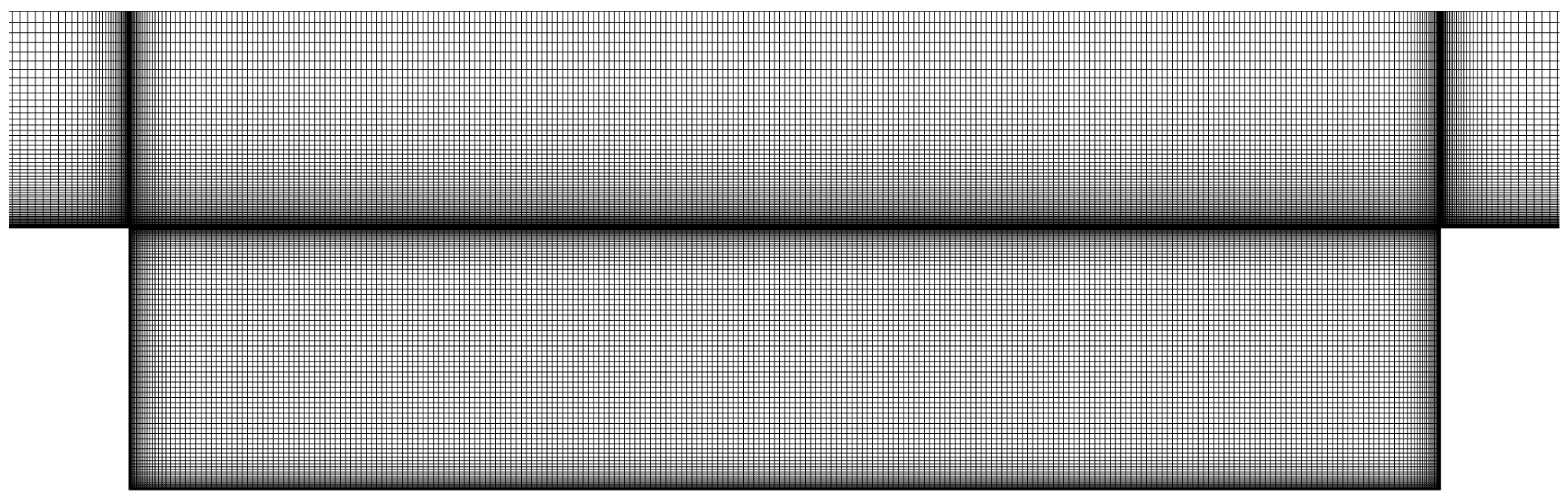
The grid is structured and contains approximately 71 million nodes. The maximum edge length—in all directions—of the hexahedral elements inside the cavity is 2 mm. Figure 3 shows the grid at the far-field boundaries and Figure 4 shows a cross-sectional plane of the grid in the cavity region. A weak adiabatic no-slip boundary condition with a wall function [21] is applied to the rig’s surfaces. The first cell height is mm. The time-averaged, dimensionless wall distance is approximately 100 on the rig’s top surface, upstream of the cavity and in the rear part of the cavity. A weak characteristic, far-field boundary condition is used for the domain inlet and outlet, whereas a free-slip boundary condition is applied to the boundaries parallel to the cavity test rig.
Figure 3.
Computational grid at the far-field boundaries for the wind tunnel model.

Figure 4.
Cross-section of the grid for the wind tunnel model in the -plane at .

3.2. Simplified Geometry
The simplified geometry is used to evaluate the effects of the elastic cavity walls on the noise generation; the computational domain for the simplified geometry is shown in Figure 5.
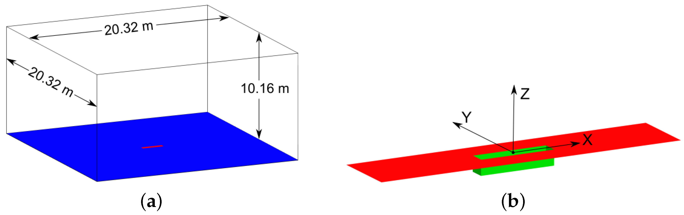
Figure 5.
(a) Computational domain for the simplified geometry. (b) Cavity and top surface. The coordinate system is defined with the origin located in the cavity centre on the plane of the top surface. Blue boundary: free-slip. Red and green boundaries: no-slip.
Figure 5.
(a) Computational domain for the simplified geometry. (b) Cavity and top surface. The coordinate system is defined with the origin located in the cavity centre on the plane of the top surface. Blue boundary: free-slip. Red and green boundaries: no-slip.

The simplified geometry is employed in lieu of the wind tunnel model for several reasons. Firstly, the computational domain is expanded in order to prevent any influence on the flow field from the wind tunnel walls. Secondly, the geometry is simplified such that only the rig’s top surface and the cavity are included. The reasons for the simplification are twofold: to reduce the number of grid points and to avert turbulence around the rig that would affect the acoustic field. The width of the top no-slip surface (red boundary in Figure 5) and the distance between the leading edge and the cavity are the same as those for the wind tunnel geometry. The top surface is symmetric about the -plane, the distance between the cavity’s rear wall and the trailing edge of the top no-slip surface is thus different from the wind tunnel geometry. The top no-slip surface is retained in the simplified geometry such that a boundary layer develops upstream of the cavity.
A free-slip boundary condition is employed for the domain’s bottom boundary (blue surface in Figure 5a), which is flush with the top no-slip surface. A weak adiabatic no-slip boundary condition with a wall function [21] is applied to the top surface (red surface in Figure 5) and to the cavity walls. A weak characteristic far-field boundary condition is used for the outlying domain boundaries.
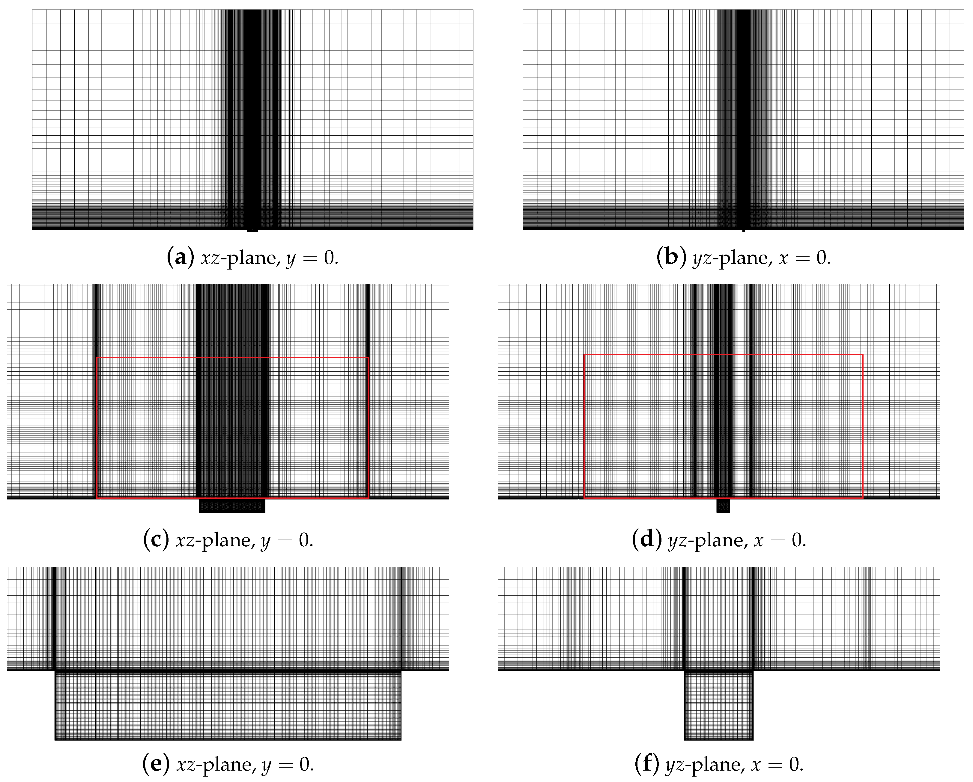
The simplified grid is similar to the wind tunnel grid in the cavity region. The maximum cell edge length is mm. The first cell height is mm, which results in on the top surface upstream of the cavity and in the rear part of the cavity. Cross-sectional planes of the whole computational domain are shown in Figure 6a,b. A grid-density box is added above the cavity; it is reaching m in the x-, y-, and z-directions, measured from the origin. Figure 6c,d show a zoomed-in view of the density box region. The maximum cell size within the density box is approximately 15 mm. In total, the grid contains approximately 43 million nodes.
Figure 6.
Cross-sectional planes of the grid for the simplified geometry. (a,b) Whole computational domain. (c,d) Density box region, marked with the red lines. (e,f) Cavity region.
Figure 6.
Cross-sectional planes of the grid for the simplified geometry. (a,b) Whole computational domain. (c,d) Density box region, marked with the red lines. (e,f) Cavity region.

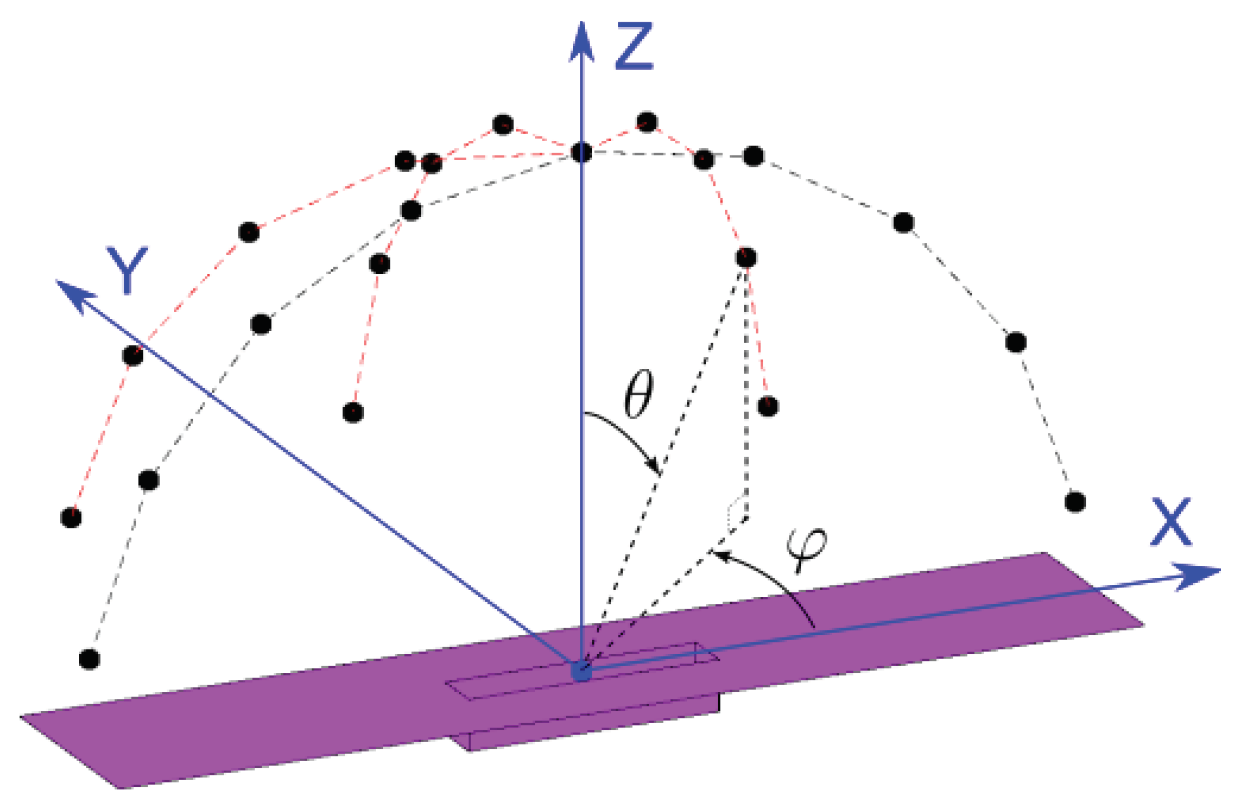
Pressure fluctuations at 21 microphones situated in the free-stream flow above the cavity are examined for the simplified geometry. All microphones are situated at a radius of m, measured from the origin. They are all situated within the grid-density box, see Figure 6c,d. The microphones are positioned at angles and , according to Figure 7. Microphones in the negative y-direction are not presented due to symmetry.
Figure 7.
Microphone positions.

3.3. Results with Rigid Cavities
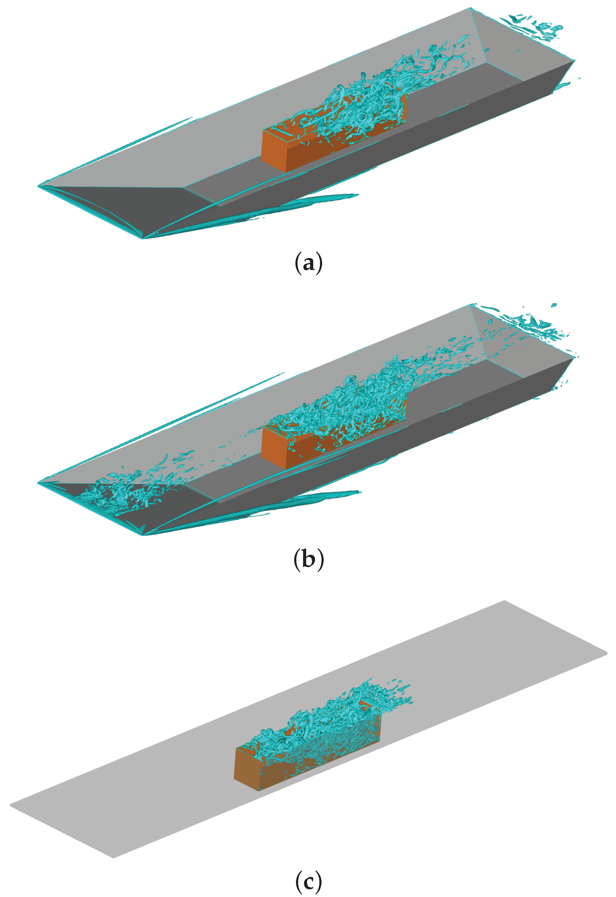
Two simulations are performed with the wind tunnel model: one with SA-DDES and one with SA-IDDES. For the simplified geometry, one simulation is undertaken with SA-IDDES. Figure 8 displays turbulent structures using iso-surfaces of the Q-criterion.
Figure 8.
(a) Wind tunnel model, SA-DDES. The visibility of the rig’s top surface and left cavity wall is turned off. (b) Wind tunnel model, SA-IDDES. (c) Simplified geometry, SA-IDDES. The visibility of the left cavity wall is turned off, and the top surface is transparent.
Figure 8.
(a) Wind tunnel model, SA-DDES. The visibility of the rig’s top surface and left cavity wall is turned off. (b) Wind tunnel model, SA-IDDES. (c) Simplified geometry, SA-IDDES. The visibility of the left cavity wall is turned off, and the top surface is transparent.

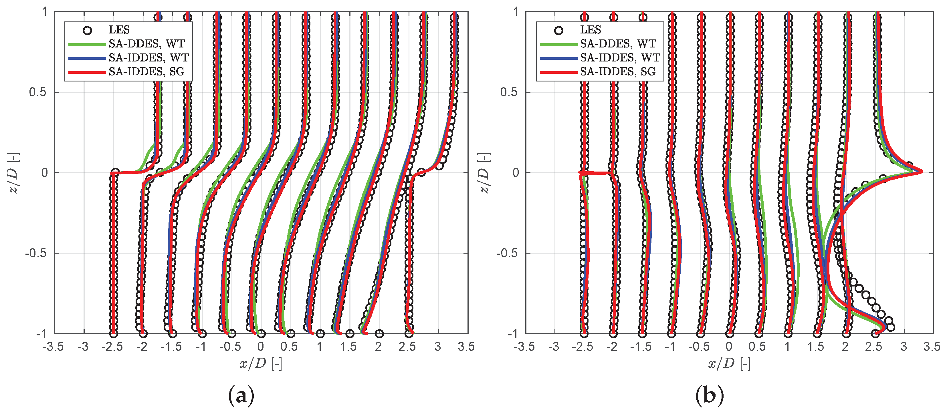
A richer content of resolved turbulence is apparent in the SA-IDDES simulation compared with the SA-DDES simulation with the wind tunnel model. It is well-known that the DDES model suffers from a slow transition from modelled turbulent stresses in the RANS mode to resolved turbulent stresses in the LES mode, the so-called grey area [22,23]. Moreover, the wedge-shaped geometry used in the wind tunnel model induces a local angle-of-attack over the leading edge, which causes a small separation bubble to form. The separation bubble is modelled in the RANS mode with SA-DDES, but it is partly resolved in the LES mode with SA-IDDES. The resolved turbulent fluctuations obtained with SA-IDDES are convected downstream to the cavity’s leading edge and spur the development of resolved turbulence in the free shear layer of the cavity. With SA-DDES, the near-wall flow upstream of the cavity is modelled in the RANS mode; as a result, there is no resolved turbulence present at the cavity’s leading edge. This further delays the development of resolved turbulence in the free shear layer, which in turn affects the flow inside the cavity. A richer content of resolved turbulence is observed with the simplified geometry using SA-IDDES compared to SA-DDES with the wind tunnel model. Figure 9 shows velocity profiles from the three simulations with the rigid cavity. The LES data by Larchêque et al. [4] are included for reference. The geometric configuration for the LES simulation was akin to the simplified geometry used here; however, only the cavity and a no-slip top surface were included. Inlet velocity profiles were used to mimic the conditions in the wind tunnel. The profiles were obtained from a boundary layer simulation since no experimental data of the velocity field were available [4]. The streamwise and vertical velocity profiles for SA-IDDES, for the wind tunnel model, and for the simplified geometry overall align with the LES profiles; the exception is the vertical velocity in the lower part of the cavity at (1.5 mm from the rear cavity wall), see Figure 9b. The SA-DDES simulation with the wind tunnel model gives a substantially different streamwise velocity profile at . The SA-DDES profiles have a larger deviation than the SA-IDDES simulations at most positions in the cavity. The deviation of the vertical velocity at is even larger with SA-DDES. The more negative vertical velocities close to the rear wall are related to the slightly higher velocities predicted further upstream of the rear wall at compared to the LES reference profiles.
Figure 9.
Time-averaged velocity profiles. WT and SG denote the wind tunnel model and the simplified geometry, respectively. (a) Streamwise velocity . (b) Vertical velocity .
Figure 9.
Time-averaged velocity profiles. WT and SG denote the wind tunnel model and the simplified geometry, respectively. (a) Streamwise velocity . (b) Vertical velocity .

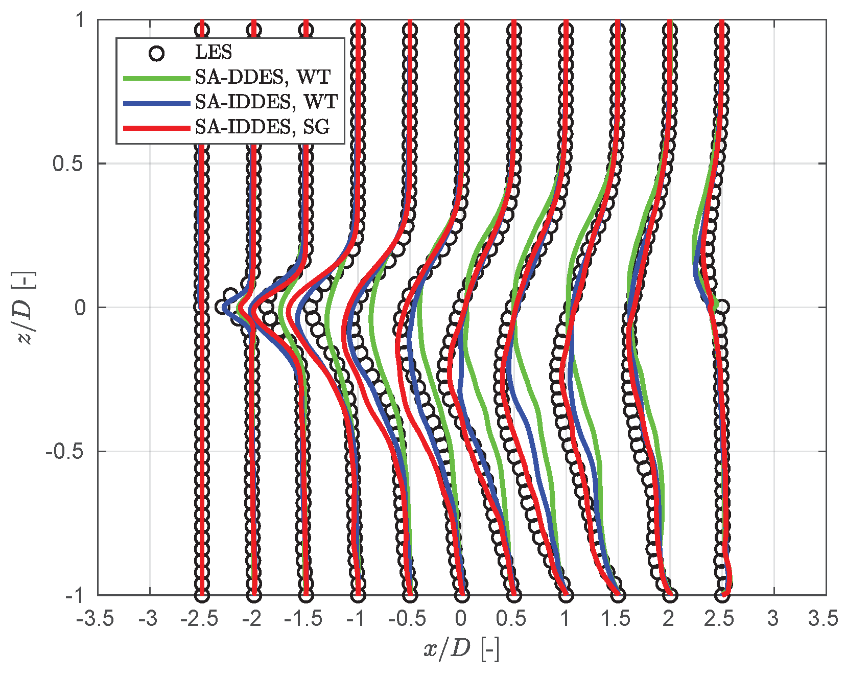
Figure 10 shows the resolved shear stress profiles. The profile at for the SA-IDDES simulation with the wind tunnel model aligns with the LES profile, whereas the other two simulations deviate. This reflects the higher turbulent content in the boundary layer for the wind tunnel model using SA-IDDES. The shear stress profiles for the wind tunnel model using SA-IDDES align reasonably well with the LES profiles at all positions. The SA-DDES simulation gives a much greater deviation from the LES profiles due to the small amount of turbulent content in the boundary layer upstream of the cavity, and also due to the grey area effect. The profiles from the simulation with the simplified geometry with SA-IDDES align better with the LES data in the rear part of the cavity than the simulations with the wind tunnel model.
Figure 10.
Time-averaged resolved shear stress . WT and SM denote the wind tunnel model and simplified geometry, respectively.
Figure 10.
Time-averaged resolved shear stress . WT and SM denote the wind tunnel model and simplified geometry, respectively.

The pressure is sampled at the same positions as the locations of the Kulite transducers, see Table 2. The sound pressure level (SPL) and overall sound pressure level (OASPL) are computed at the probes. The SPL is defined as:
The reference sound pressure is Pa. The power spectral density is computed using Welch’s method [24], the MATLAB function pwelch [25] is employed. A Hanning window is used, and the signals from the CFD simulations are divided into 16 segments. The experimental data signal is much longer—approximately 3.4 s—and it is divided into 96 segments. The window size in terms of physical time is approximately 70 ms for both the experimental and the CFD signals. A window overlap of 50 percent is used.
The OASPL is computed as:
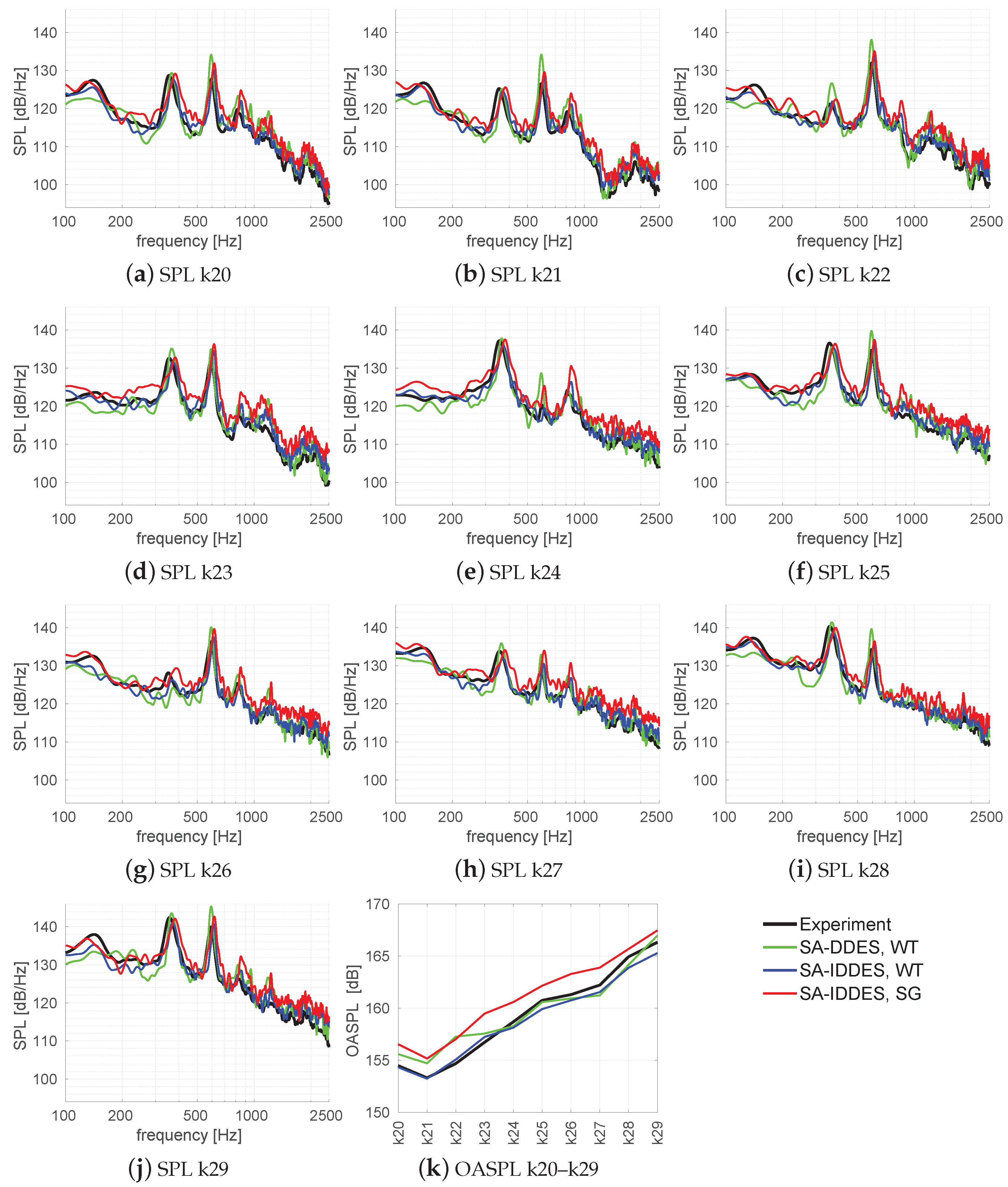
Here, the subscript denotes the root mean square value of the pressure fluctuations , which is defined as the difference between the local instantaneous pressure and the local time-averaged pressure. The Rossiter mode frequencies are identified from the peak value positions in the power spectra. The frequencies can differ by a few Hertz between the probe positions. The frequencies are computed as the mean frequency obtained at the probes; the frequencies are given in Table 3. The SPL and OASPL at probes k20–k29 are given in Figure 11 for the three simulations and for the experimental data.
Table 3.
Rossiter mode frequencies. WT and SG denote the wind tunnel model and simplified geometry, respectively.
Table 3.
Rossiter mode frequencies. WT and SG denote the wind tunnel model and simplified geometry, respectively.
| Mode | Experimental (Hz) | SA-DDES, WT (Hz) | SA-IDDES, WT (Hz) | SA-IDDES, SG (Hz) |
|---|---|---|---|---|
| 1 | 140 | - | 138 | 130 |
| 2 | 352 | 365 | 370 | 381 |
| 3 | 592 | 592 | 611 | 614 |
| 4 | 812 | 822 | 854 | 852 |
Figure 11.
(a–j) SPL at probes k20–k29. (k) OASPL at probes k20–k29. Here, WT and SG denote the wind tunnel model and simplified geometry, respectively.
Figure 11.
(a–j) SPL at probes k20–k29. (k) OASPL at probes k20–k29. Here, WT and SG denote the wind tunnel model and simplified geometry, respectively.

As seen in Figure 11, the first Rossiter mode is poorly resolved in the SA-DDES simulation. An increase in SPL can be seen at several probes, but the peak values are obscured. Rossiter modes 2–4 are better predicted in terms of frequency with the use of SA-DDES compared with SA-IDDES. However, SA-DDES overpredicts the magnitude of the Rossiter modes at most probes. An example is seen for the 3rd Rossiter mode at probe k24, Figure 11e; SA-DDES gives a significant power peak, whereas the power of this mode is small with SA-IDDES, which aligns with the experimental data. The 3rd Rossiter frequency is apparent with SA-IDDES for the simplified geometry at probe k24 as well. As seen in Figure 11, the simplified geometry gives generally higher mode powers—especially for the 3rd and 4th Rossiter modes—and broadband noise than the wind tunnel model. It should be mentioned that the magnitudes in the SPL spectra should not be considered as exact; the reasons are both numerical and physical. Welch’s method provides an estimation of the PSD. The confidence levels can easily be computed but are not shown in Figure 11. The 99 percent confidence bounds are approximately ±1.15 dB for the experimental SPL and ±2.85 dB for the CFD-based spectra. Increasing the confidence level results in a lower frequency resolution, which is not desirable here. An analysis with a higher confidence level (not shown here) shows that the obtained differences in Figure 11 are significant. The physical aspect, as previously mentioned, is that neither the Rossiter mode amplitudes nor the frequencies are constant over time.
The OASPL for the simplified geometry using SA-IDDES, as seen in Figure 11k, consistently shows higher levels than simulations with the wind tunnel model. This can be attributed to the lower level of resolved turbulence in the boundary layer upstream of the cavity. The OASPL for the wind tunnel model with SA-IDDES aligns reasonably with the experimental data. In the front part of the cavity, the OASPL agrees with the experiment, whereas the OASPL is approximately 1 dB lower in the rear-most part of the cavity. The OASPL using SA-DDES and the wind tunnel model gives a higher deviation in comparison with the experimental data.
In summation, the grey area effect is less apparent with SA-IDDES, which provides a better prediction of the power levels. On the other hand, SA-DDES predicts the Rossiter mode frequencies better—first mode excluded—compared to the experimental data. Furthermore, the velocity and shear stress profiles using SA-IDDES align better than SA-DDES with the LES data. For the ensuing FSI simulation, SA-IDDES is employed. It is evident that the flow simulation methods can be improved to better predict the Rossiter modes. An accurate prediction of the Rossiter modes is especially important for an elastic cavity because of the interaction with structural eigenmodes. However, in this numerical study, the exact prediction of the Rossiter modes is not paramount since no empirical data regarding structural deformations are available. The simulation with the simplified geometry presented in this section is used as the reference case for the FSI simulation.
4. Finite Element Model and the Modal Representation
The structural finite element (FE) model of the cavity is introduced, followed by a description of the modal representation.
4.1. Finite Element Model
The aeroelasticity of the M219 cavity has not been tested in a wind tunnel. A rigid cavity was considered in the test by Henshaw [9], and no structural model associated with the test is available. For this numerical study, it is desired that the structure is stimulated such that significant structural vibrations are obtained; however, the magnitude of the vibrations should be realistic. A real cavity structure—for example, a weapon bay—is often complex, and it is not obvious what could be considered as a realistic vibration level. Moreover, the vibration level may differ substantially between different weapon bay designs. Here, the structure is made as simple as possible, representing a cavity made of aluminium sheets with uniform properties. A material thickness of 1.5 mm is used. This resulted in a maximum displacement of approximately mm for the floor and the side walls during the FSI simulation presented in Section 5. The maximum displacement is 0.24 percent of the cavity length, which falls within the range considered to be reasonable for this study. Furthermore, in this study, it is undesirable for any structural eigenfrequency to coincide with a Rossiter mode frequency. Therefore, in choosing the thickness—which affects the eigenfrequencies—it is ascertained that the structural eigenfrequencies are separated from the Rossiter frequencies.
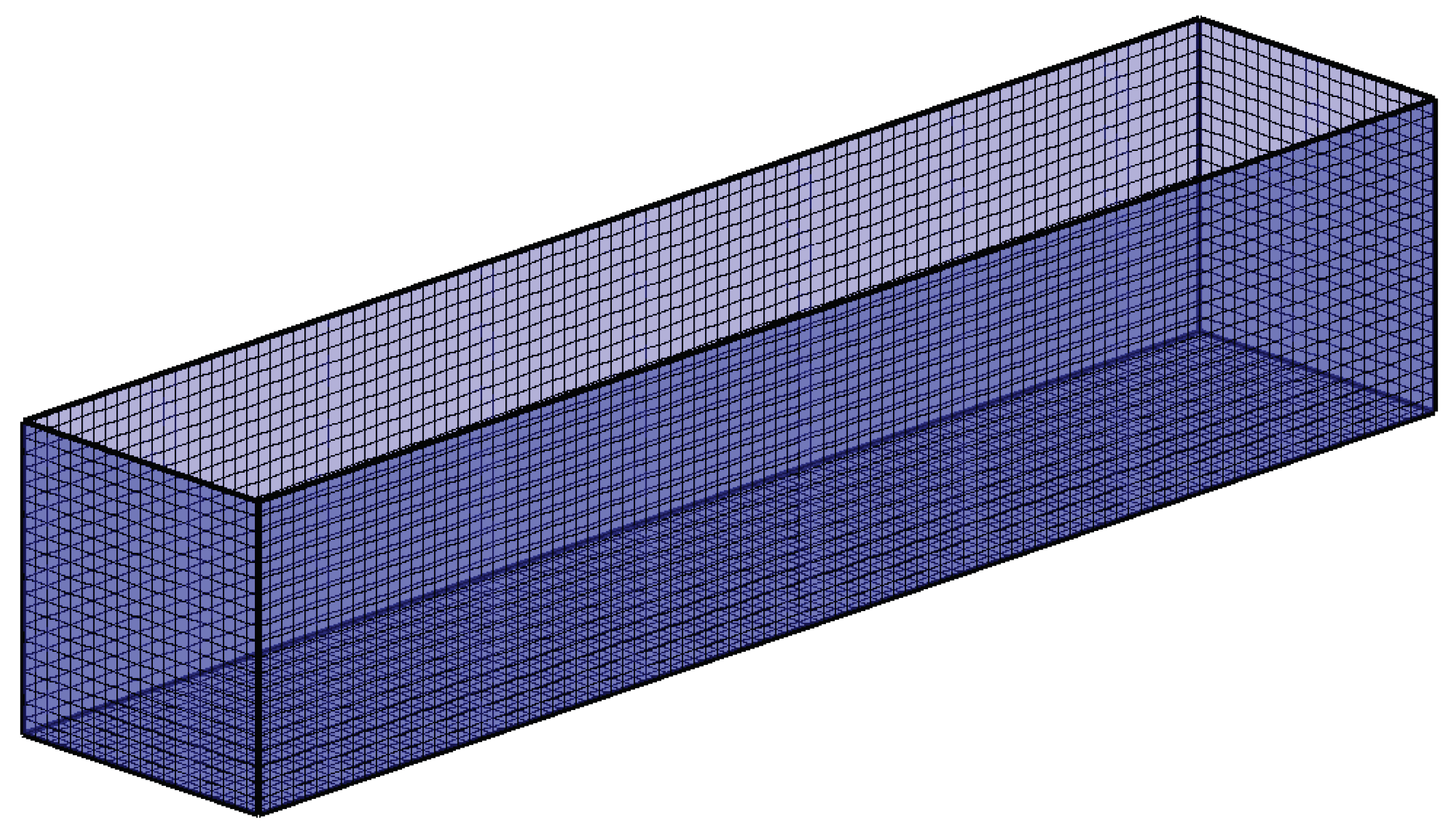
The FE analysis software MSC Nastran [26] is employed to formulate and solve the structural eigenvalue problem. The FE model consists of 6800 quadrilateral first-order shell elements (called CQUAD4 in MSC Nastran). All elements are squares, with edge lengths of mm. The FE model is shown in Figure 12.
Young’s modulus is set to , Poisson’s ratio is , and the material density is 2700 . The structural damping is set to zero; hence, only aerodynamic damping acts on the system.
The maximum resolved frequency is calculated as , where n is the number of elements per wavelength, and is the speed of sound in the fluid. At least four elements are required to capture a wave; however, adding a few elements significantly increases the resolution. For example, setting gives Hz, which is well beyond the highest considered frequency. The FE grid resolution together with the element type are important for the accuracy and resolution of the normal mode shapes. The grid points have six degrees of freedom. All six degrees of freedom are constrained at the grid points that are connected to the top surface at .
Figure 12.
Finite element model.

4.2. Modal Representation of the Structural Model
The eigenvalue problem of the FE model is solved using the real eigenvalue analysis solver in MSC Nastran [26] (called SOL 103 in Nastran). The natural frequencies, generalised masses, and the normal mode shapes are then used by the modal-based solver. In M-Edge, each normal mode shape is stored in a so-called perturbation grid. A perturbation grid is the CFD grid deformed according to a normal mode shape. The normal mode shapes are mapped onto the CFD grid using the shell projection tool in the software Scope [27]. The first 50 normal mode shapes are included in the modal representation of the cavity, spanning frequencies of 468–2280 Hz. The frequencies for all modes are given in Table 4. Normal mode shapes 1 and 50 are shown in Figure 13.
Figure 13.
Illustration of the lowest and highest normal mode shapes included in the modal representation. (a) Mode 1. (b) Mode 50.
Figure 13.
Illustration of the lowest and highest normal mode shapes included in the modal representation. (a) Mode 1. (b) Mode 50.

Table 4.
Structural eigenfrequencies.
| Mode | f (Hz) | Mode | f (Hz) | Mode | f (Hz) | Mode | f (Hz) |
|---|---|---|---|---|---|---|---|
| 1 | 468 | 14 | 949 | 27 | 1546 | 40 | 2026 |
| 2 | 509 | 15 | 956 | 28 | 1587 | 41 | 2082 |
| 3 | 577 | 16 | 992 | 29 | 1642 | 42 | 2087 |
| 4 | 646 | 17 | 1042 | 30 | 1664 | 43 | 2087 |
| 5 | 675 | 18 | 1087 | 31 | 1665 | 44 | 2120 |
| 6 | 702 | 19 | 1107 | 32 | 1732 | 45 | 2163 |
| 7 | 759 | 20 | 1139 | 33 | 1762 | 46 | 2177 |
| 8 | 801 | 21 | 1214 | 34 | 1823 | 47 | 2214 |
| 9 | 812 | 22 | 1242 | 35 | 1849 | 48 | 2255 |
| 10 | 836 | 23 | 1278 | 36 | 1893 | 49 | 2265 |
| 11 | 841 | 24 | 1350 | 37 | 1942 | 50 | 2280 |
| 12 | 877 | 25 | 1363 | 38 | 1992 | ||
| 13 | 933 | 26 | 1446 | 39 | 2005 |
5. Results with the Elastic Cavity
5.1. Analysis of Noise in the Free-Stream Flow
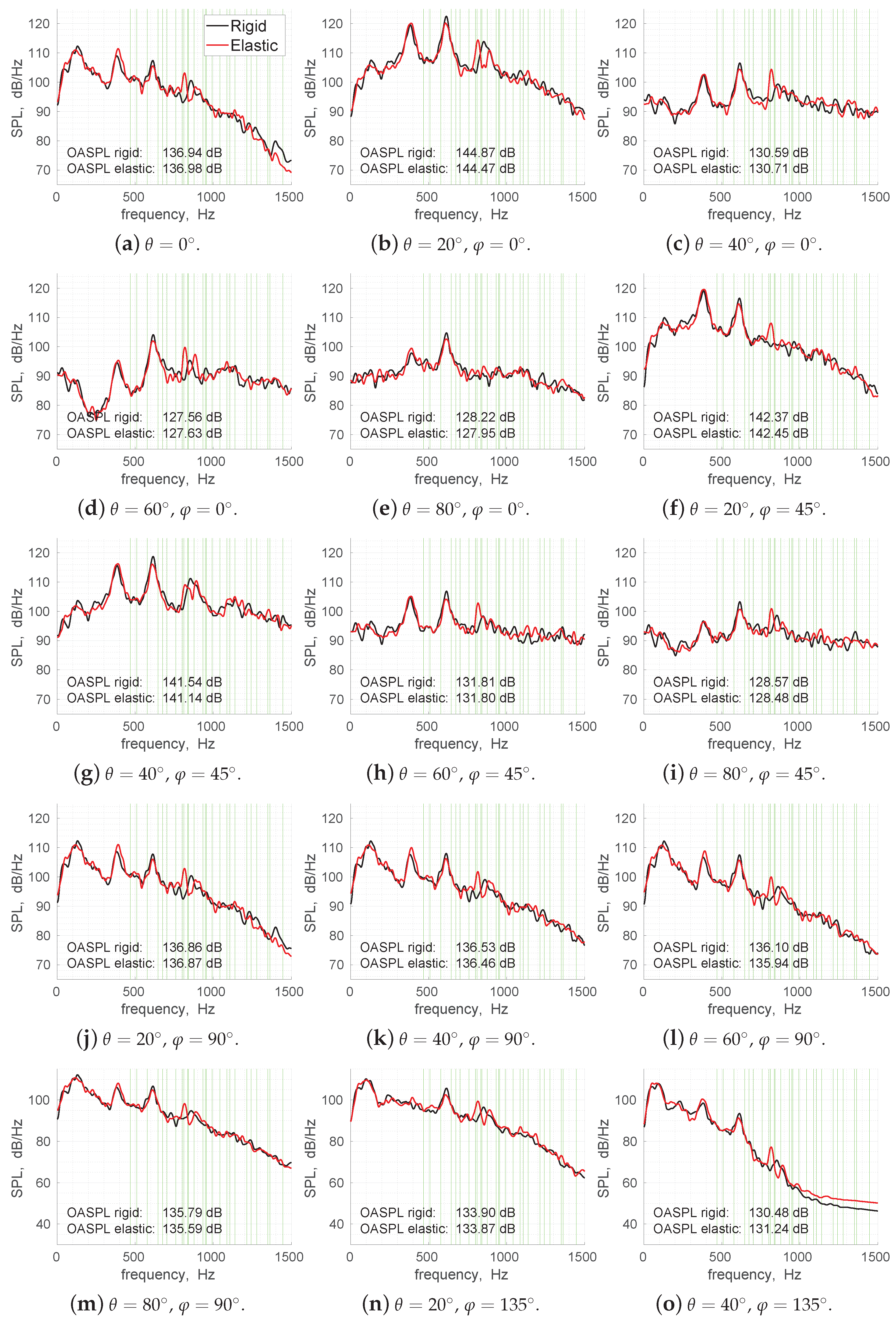
Figure 14 and Figure 15 show the SPL and the OASPL at the microphones, see Figure 7. The same methods as those previously described are used for the computation of the SPL and the OASPL; this means that the confidence level is dB. An analysis with a higher confidence level was undertaken (not shown), which showed that the differences in the peak magnitudes discussed henceforth are significant.
Firstly, for the microphones upstream of the cavity at –, Figure 14o and Figure 15a–f, the SPLs are flattened at high frequencies. This can be attributed to limited pressure fluctuations. In other words, the differences are numerical rather than physical.
The SPL spectra at the microphones showed that the four Rossiter modes are altered by the interaction between the fluid and the structure. The power of the 1st Rossiter mode at 130 Hz is slightly lower for the elastic cavity at most of the microphones. This is most apparent in Figure 14c,g,h. The spectra show the opposite trend for the 2nd Rossiter mode at 381 Hz, namely an increase in power for the elastic cavity. This can be clearly seen in Figure 14j–m. The power of the 3rd Rossiter mode at 614 Hz is lower for the elastic cavity at most of the microphones. The largest differences are obtained in Figure 14g–i. A clear and consistent difference between the rigid and the elastic cavity simulation is obtained for frequencies between 800 Hz and 900 Hz. The 4th Rossiter mode is within this range, namely at 852 Hz. In addition to the Rossiter mode, there is another peak at a frequency of Hz for the rigid cavity case. This peak was identified through an analysis with a higher frequency resolution, which is not shown here. The power of the 4th Rossiter mode is depleted at most microphones for the elastic cavity. Concurrently, the peak at 900 Hz is intensified, and a tone is induced at 816 Hz; these changes are clearly seen in Figure 14d.
The analysis using a higher frequency resolution (not shown here) revealed a few more tones at higher frequencies, which are absent in the rigid cavity. A tone at 1139 Hz and another at 1184 Hz were obtained. The former coincides with a structural eigenfrequency, whereas the latter does not. Another tone was identified at 1354 Hz, which is close to a structural eigenfrequency. These tones are further investigated in the ensuing SPOD analysis.
Figure 14 and Figure 15 show that none of the Rossiter modes coincides with any structural eigenfrequency. However, the 4th Rossiter mode is close to normal mode shape 11 (see Table 4), which is merely 11 Hz below the 4th Rossiter mode. The tone induced by the elastic cavity at 816 Hz is close to normal mode shape 9 at 812 Hz.
The OASPL at the microphones are given in Figure 14 and Figure 15. The difference in the OASPL between the rigid and elastic cavities is relatively small, approximately 1 dB at most. The small difference between the rigid and the elastic cavities does not mean that the elasticity can be neglected in a cavity noise analysis because it does not describe the spectral content. The highest OASPL is approximately 145 dB and is found at and ; see Figure 14b.
The analysis performed here should ideally be performed with microphones located further away from the cavity, where the strong pressure fluctuations will have abated further. However, this would demand a finer grid resolution further away from the cavity.
Figure 14.
SPL and OASPL at the microphones. Green vertical lines mark the structural eigenfrequencies.
Figure 14.
SPL and OASPL at the microphones. Green vertical lines mark the structural eigenfrequencies.

Figure 15.
SPL at the microphones. Green vertical lines mark the structural eigenfrequencies.

5.2. Spectral Proper Orthogonal Decomposition of Wall Pressures and Displacements
The spectral proper orthogonal decomposition (SPOD) method [28,29] is employed for the analysis of cavity wall pressure fluctuations and wall displacements d; the pressure fluctuations and the displacements are analysed separately. Pressure fluctuations from the rigid cavity are also analysed for reference. The SPOD method extracts coherent features from the turbulent flow; the turbulent structures are represented by a set of deterministic modes, which represent the energy. Each mode oscillates at a single frequency and evolves coherently in both space and time [29].
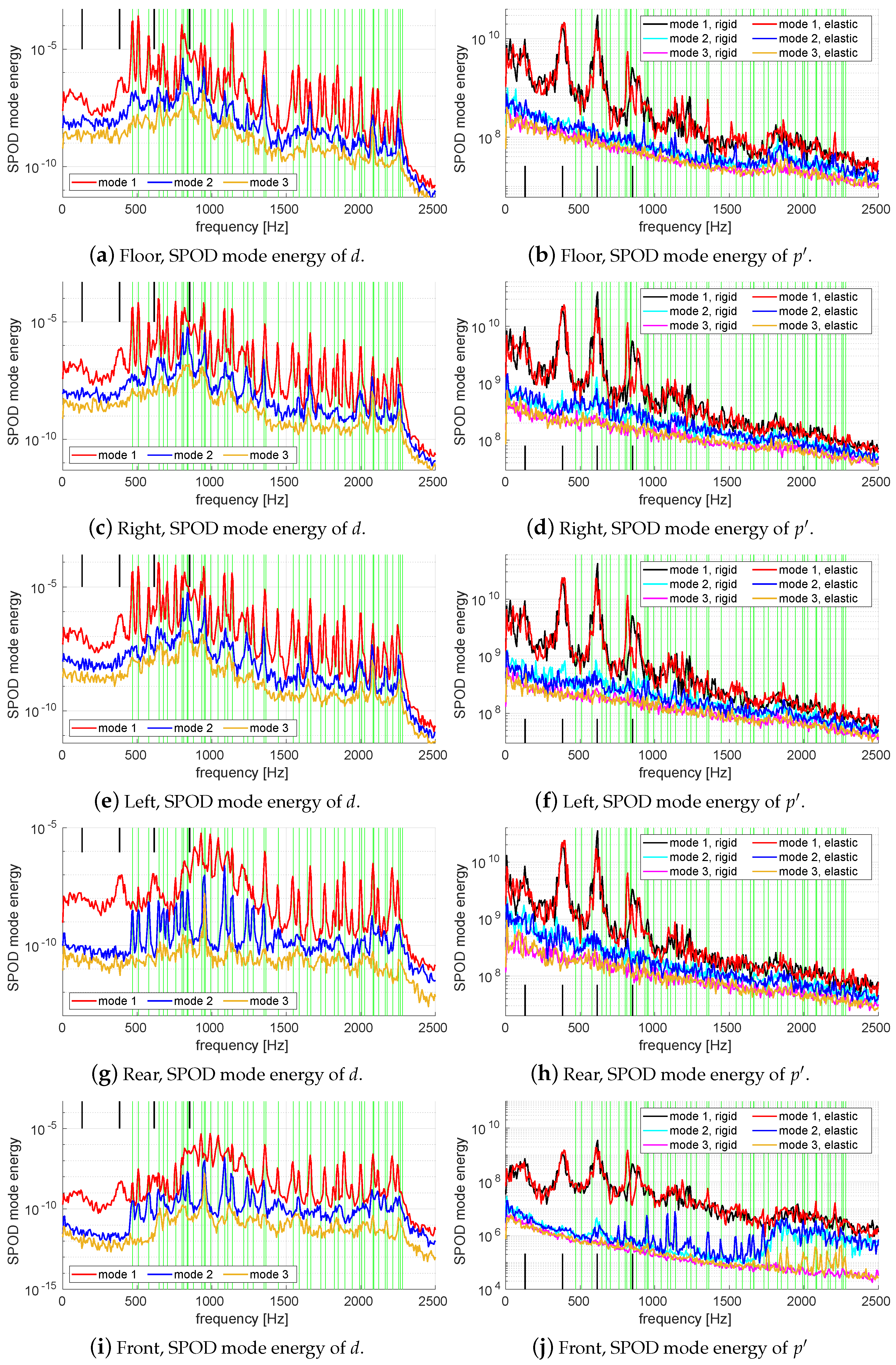
The data are divided into six blocks, each containing samples (time steps). A Hanning window and a 50 percent overlap are used. This results in six modes with a frequency resolution (also called bin size) of approximately Hz. It should be mentioned that it would be desirable to use more than six blocks for the SPOD analysis; it would significantly increase the confidence level in the spectral estimate for each bin. However, it would concurrently increase the bin size, which would result in a substantial leakage between the bins. In other words, nearby energy peaks would meld together. This trade-off between confidence and bin size must always be considered. Here, for both the displacements and the pressure fluctuations, several energy peaks are near each other, and the bin size must be sufficiently small to avert leakage between the bins. The main purpose of this analysis is to identify specific tones and structural oscillatory frequencies rather than to accurately determine the spectral energies.
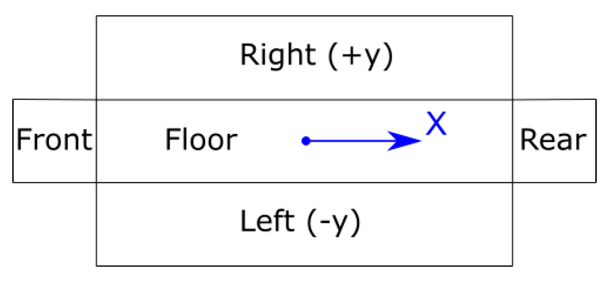
The five cavity walls are analysed separately; for clarity, the naming of the cavity walls is shown in Figure 16. The SPOD mode energies of the first three modes for d and are shown in Figure 17. The remaining modes mostly consist of broadband noise.
Figure 16.
Naming of the cavity surfaces. The side walls are folded outwards.

Figure 17.
SPOD mode energy for displacements d (left column) and pressure fluctuations (right column). Green vertical lines mark the structural eigenfrequencies. Black vertical lines mark the Rossiter frequencies.
Figure 17.
SPOD mode energy for displacements d (left column) and pressure fluctuations (right column). Green vertical lines mark the structural eigenfrequencies. Black vertical lines mark the Rossiter frequencies.

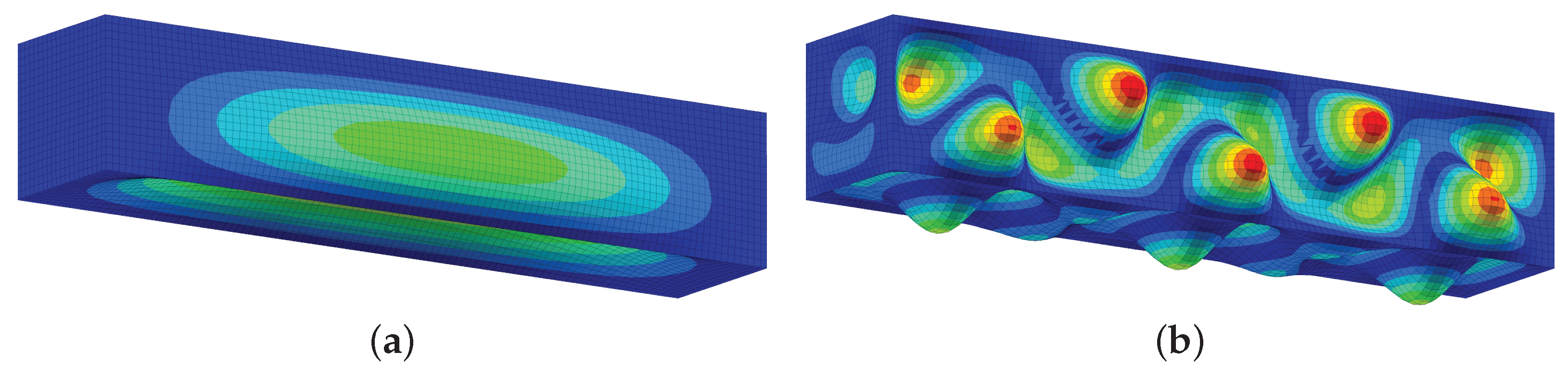
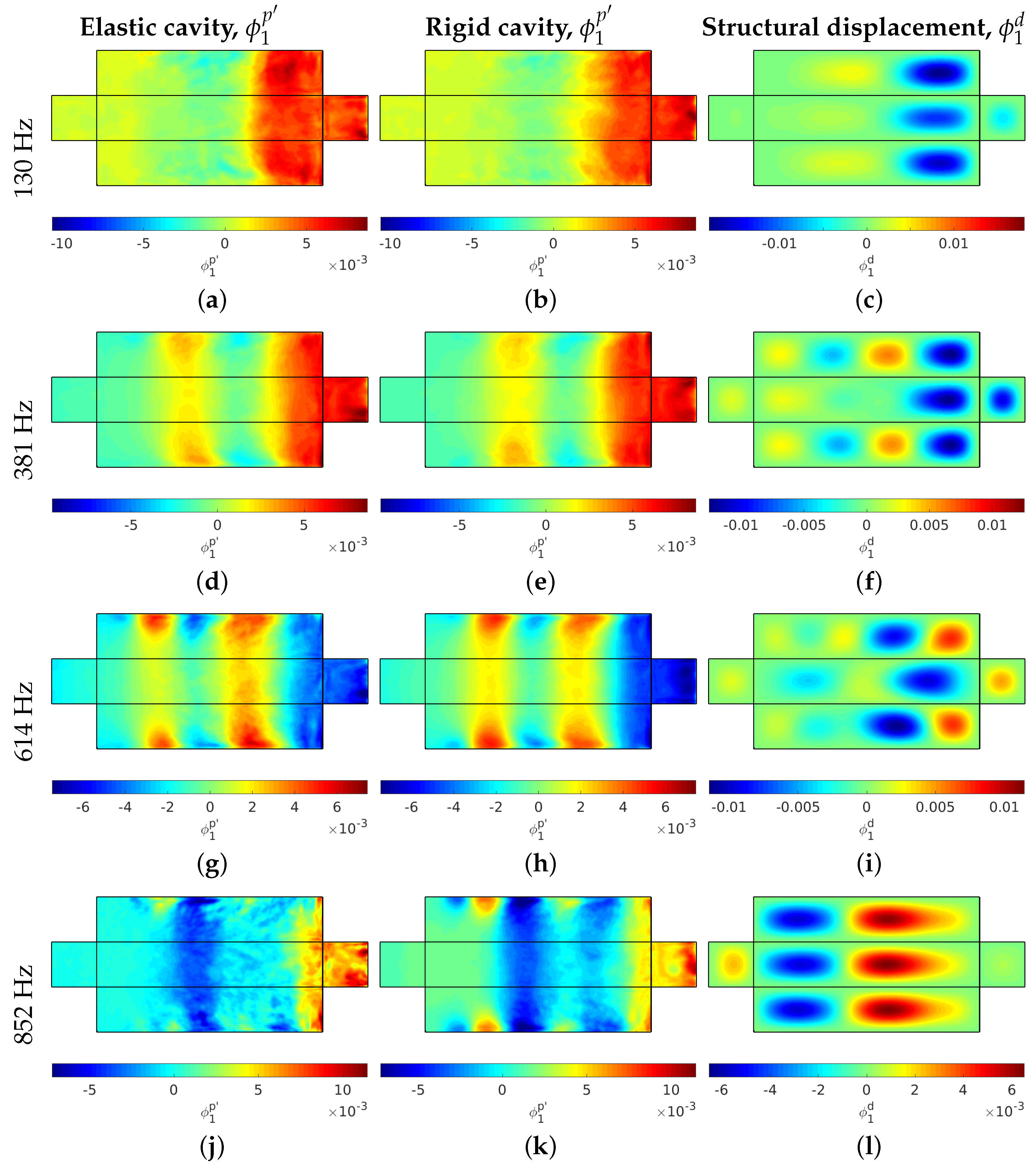
Figure 18.
The 1st SPOD modes for pressure fluctuations of the elastic cavity (left column), rigid cavity (middle column), and for displacements (right column) at the Rossiter frequencies.
Figure 18.
The 1st SPOD modes for pressure fluctuations of the elastic cavity (left column), rigid cavity (middle column), and for displacements (right column) at the Rossiter frequencies.

The SPOD mode energy spectra of the pressure fluctuations (right column in Figure 17) are similar to the spectra obtained at the microphones in the previous section. For the elastic cavity, the energy peak at the 4th Rossiter mode is depleted on all five walls, and the induced tone at 816 Hz is obtained on all five walls. In addition to the tones obtained at the microphones, several others can be identified here. Figure 17b shows additional tones at Hz. These are most apparent on the cavity floor. A few of these coincide with structural eigenfrequencies, whilst others do not. Spectral POD modes 2–3 for mostly contain broadband noise. However, the energy spectra for SPOD modes 2–3 for the front wall are an exception, as can be seen in Figure 17j. Additional tones that coincide with structural eigenfrequencies are obtained. These tones are induced by the elastic walls, the waves propagate upstream and impinge upon the front wall.
Figure 19.
The 1st SPOD modes for pressure fluctuations of the elastic cavity (left column), rigid cavity (middle column), and for displacements (right column) at frequencies Hz.
Figure 19.
The 1st SPOD modes for pressure fluctuations of the elastic cavity (left column), rigid cavity (middle column), and for displacements (right column) at frequencies Hz.

The left column in Figure 17 shows the SPOD mode energy spectra of the structural displacements. It is evident that all the fifty structural eigenmodes included are excited. The impact of the 2nd Rossiter mode at 381 Hz is clearly visible. An energy increase is also obtained at about 130 Hz, which is at the 1st Rossiter mode. The first and second Rossiter modes are below the lowest structural eigenfrequency. However, the strength of the Rossiter modes cause the structure to oscillate at the corresponding frequencies. At frequencies above the highest structural eigenfrequency, the SPOD mode energies decay.
The 1st SPOD modes for displacement and pressure fluctuations , for both the rigid and the elastic cavity at the Rossiter frequencies, are displayed in Figure 18. Corresponding figures for the previously discussed frequencies, namely Hz, are shown in Figure 19. The SPOD modes for the elastic cavity are found in the first column, the second column shows the corresponding modes for the rigid cavity; these modes are approximately in-phase and displayed with equal scales. The third column shows the SPOD modes of the structural displacement . These modes are not necessarily showed in-phase nor with the actual phase shift in relation to .
The SPOD modes of the pressure fluctuations for Rossiter modes 1–3, Figure 18, are similar for the elastic and the rigid cavity. However, the 4th Rossiter mode is noticeably weaker for the elastic cavity. This is in line with previous observations. The SPOD mode energy spectra and the SPL spectra for the elastic cavity showed decreased energy at this frequency. This implies that the energy transfer from the fluid to the structure is significant at the 4th Rossiter frequency.
The SPOD modes for the other tones, Figure 19, show a clear pattern. The modes are more distinct for the elastic cavity than for the rigid cavity. This is to be expected based on the SPOD mode energy spectra and, in some cases, also the SPL spectra. Distinctive pressure waves at these frequencies are absent or weak in the rigid cavity, whereas waves are induced by the interaction between the fluid and the structure at the specific frequencies in the elastic cavity.
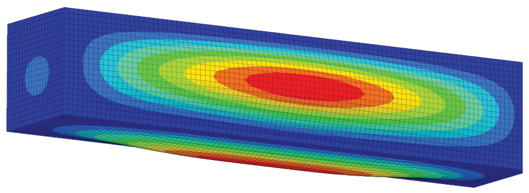
Not all structural normal mode shapes are shown here. However, in cases where they coincide with or are close to the SPOD modes, there are similarities, but not necessarily on all five walls. For example, at 2210 Hz (Figure 19r), the right, left, front, and rear walls are similar to normal mode shape 47 (see Table 4). However, normal mode shape 47 does not have the zigzag pattern of high and low values, as seen for the cavity floor in Figure 19r. The SPOD mode at 816 Hz is similar to the normal mode shape at 812 Hz (Mode 9, Table 4), which is shown in Figure 20.
Figure 20.
Structural normal shape of Mode 9.

6. Summary and Conclusions
The effects of elastic cavity walls on flow noise generation are investigated using SA-IDDES and a modal formulation for structural analysis. Furthermore, a flow solver validation is undertaken, where SA-IDDES and SA-DDES are used in combination with a wall function and a rigid cavity. The M219 cavity geometry, which has been tested in a wind tunnel is employed for the flow solver validation. The results are compared with the wind tunnel data and LES data. The results are also compared with results using a simplified geometric model. The simplified geometry consistently produced a higher overall sound pressure level (OASPL) at the probes inside the cavity; this is likely due to the lower level of resolved turbulence in the boundary layer upstream of the cavity. Furthermore, most Rossiter frequencies and sound pressure levels (SPL) are higher for the simplified geometry. The flow over the wind tunnel model’s leading edge detaches and a small separation bubble is formed. This affects the boundary layer upstream of the cavity and thereby the cavity flow characteristics. This leads to lower and more accurate SPL and OASPL compared to the simplified geometry, where less resolved turbulence is present in the boundary layer at the cavity leading edge.
A comparison of the resulting flow field using SA-DDES and SA-IDDES with the wind tunnel model shows that more resolved turbulence is present in the early stage of the free shear layer with SA-IDDES than with SA-DDES. The SA-DDES turbulence model predicts the 2nd, 3rd, and 4th Rossiter modes better than SA-IDDES in terms of frequency, but completely fails to resolve the 1st Rossiter mode. Furthermore, SA-DDES overpredicts the SPL at the Rossiter frequencies, and the OASPL is less accurate compared to the wind tunnel data. The 2nd, 3rd, and 4th Rossiter frequencies are overpredicted by SA-IDDES. On the other hand, the peak magnitudes of the SPL spectra align better with the experimental data. The OASPL agrees with the experimental data in the front part of the cavity, whilst it is approximately 1 dB lower in the rear-most part of the cavity. Comparisons with LES velocity and shear stress profiles showed that SA-IDDES aligns better with the profiles than SA-DDES.
The FSI simulation of the elastic cavity is performed with the simplified geometry. The results are compared with a reference simulation of the rigid cavity with the simplified geometry. Pressure fluctuations are recorded at 21 microphones located two cavity lengths away from the cavity in a spherical pattern. Spectral analysis of the micropophone signals shows a distinct tone at 816 Hz, which is not obtained for the rigid reference case. The power of the 4th Rossiter mode is concurrently depleted at most microphones. The induced tone at 816 Hz is 36 Hz below the 4th Rossiter mode; moreover, it is close to a structural eigenfrequency at 812 Hz. Furthermore, changes to the SPL are obtained for the first three Rossiter modes. The OASPL at the microphones are similar for the elastic and the rigid cavity.
Spectral proper orthogonal decomposition (SPOD) is employed for analysis of the cavity wall pressure fluctuations and for the wall displacements. The phenomenon at the 4th Rossiter mode frequency is also obtained in the SPOD mode energy spectra for the pressure fluctuations. A tone at 816 Hz is observed, and the energy peak at the 4th Rossiter mode is depleted. This implies a substantial energy transfer between the fluid and the structure at the 4th Rossiter mode frequency. Additional high-frequency tones above 1000 Hz are found in the SPOD mode energy spectra for the cavity’s front wall, which coincide with structural eigenfrequencies. The SPOD mode energy spectra for the wall displacements show that all included normal mode shapes of the modal representation are excited.
Author Contributions
Conceptualisation, S.N., H.-D.Y., A.K. and S.A.; data curation, S.N.; formal analysis, S.N.; funding acquisition, S.A.; investigation, S.N.; methodology, S.N.; project administration, S.A.; resources, S.N. and S.A.; software, S.N. and A.K.; supervision, H.-D.Y., A.K. and S.A.; validation, S.N.; visualisation, S.N.; writing—original draft, S.N.; writing—review and editing, H.-D.Y., A.K. and S.A. All authors have read and agreed to the published version of the manuscript.
Funding
This work was funded by the Swedish Governmental Agency for Innovation Systems (VINNOVA), the Swedish Defence Materiel Administration (FMV), the Swedish Armed Forces within the National Aviation Research Programme (NFFP, Contract No. 2019-02779), and Saab Aeronautics.
Institutional Review Board Statement
Not applicable.
Informed Consent Statement
Not applicable.
Data Availability Statement
Not applicable.
Acknowledgments
Hua-Dong Yao obtained support in the computations/data handling, which were enabled by resources provided by the Swedish National Infrastructure for Computing (SNIC) at Vera and Tetralith, partially funded by the Swedish Research Council through grant agreement no. 2018-05973. Hua-Dong Yao also received support from the Chalmers Foundation project on Hydro/Aerodynamics initiative.
Conflicts of Interest
The authors declare no conflict of interest.
Abbreviations
The following abbreviations are used in this manuscript:
| CFD | computational fluid dynamics |
| DDES | delayed detached-eddy simulation |
| FE | finite element |
| FSI | fluid–structure interaction |
| IDDES | improved delayed detached-eddy simulation |
| LES | large-eddy simulation |
| OASPL | overall sound pressure level |
| RANS | Reynolds-averaged Navier–Stokes |
| SA | Spalart–Allmaras |
| SPL | sound pressure level |
| SPOD | spectral proper orthogonal decomposition |
| PSD | power spectral density |
References
- Rossiter, J.E. Wind-Tunnel Experiments on the Flow over Rectangular Cavities at Subsonic and Transonic Speeds; Reports and Memoranda No. 3438, Ministry of Aviation; Her Majesty’s Stationery Office: London, UK, 1966.
- Peng, S.H. Simulation of Turbulent Flow Past a Rectangular Open Cavity Using DES and Unsteady RANS. In Proceedings of the 24th AIAA Applied Aerodynamics Conference, San Francisco, CA, USA, 5–8 June 2006. [Google Scholar]
- Lawson, S.J.; Barakos, G.N. Review of numerical simulations for high-speed, turbulent cavity flows. Prog. Aerosp. Sci. 2011, 47, 186–216. [Google Scholar] [CrossRef]
- Larchevêque, L.; Sagaut, P.; Lê, T.H.; Comte, P. Large-eddy simulation of a compressible flow in a three-dimensional open cavity at high Reynolds number. J. Fluid Mech. 2004, 516, 265–301. [Google Scholar] [CrossRef]
- Luo, K.; Xiao, Z. Improved Delayed Detached-Eddy Simulation of Transonic and Supersonic Cavity Flows. In Progress in Hybrid RANS-LES Modelling; Notes on Numerical Fluid Mechanics and Multidisciplinary Design; Springer: Cham, Switzerland, 2015; Volume 130, pp. 163–174. [Google Scholar]
- Peng, S.H.; Leicher, S. DES and Hybrid RANS-LES Modelling of Unsteady Pressure Oscillations and Flow Features in a Rectangular Cavity. In Advances in Hybrid RANS-LES Modelling; Notes on Numerical Fluid Mechanics and Multidisciplinary Design; Springer: Cham, Switzerland, 2008; Volume 97, pp. 132–141. [Google Scholar]
- Allen, R.; Mendonça, F. RANS and DES turbulence model predictions of noise on the M219 cavity at M = 0.85. Int. J. Aeroacoust. 2005, 4, 135–151. [Google Scholar] [CrossRef]
- Łojec, P.; Czajka, I.; Gołaś, A.; Suder-Dębska, K. Influence of the Elastic Cavity Walls on Cavity Flow Noise. Vib. Phys. Syst. 2021, 32, 2021109. [Google Scholar]
- Henshaw, M.J.d.C. Verification and Validation Data for Computational Unsteady Aerodynamics; M219 Cavity Case Technical Report; British Aerospace (Operations) Ltd., Military Aircraft and Aerostructures: Brough, UK, 1991. [Google Scholar]
- Gritskevich, M.S.; Garbaruk, A.V.; Menter, F.R. A Comprehensive Study of Improved Delayed Detached Eddy Simulation with Wall Functions. Flow Turbul. Combust 2017, 98, 461–479. [Google Scholar] [CrossRef]
- Mockett, C.; Fuchs, M.; Thiele, F. Progress in DES for wall-modelled LES of complex internal flows. Comput. Fluids 2012, 65, 44–55. [Google Scholar] [CrossRef]
- Eliasson, P. Edge: A Navier-Stokes Solver for Unstructured Grids. In Finite Volumes for Complex Applications III; CP849; Kogan Page: London, UK, 2002; pp. 527–534. [Google Scholar]
- Eliasson, P.; Weinerfelt, P. Recent applications of the flow solver Edge. In Proceedings of the 7th Asian CFD Conference, Bangalore, India, 26–30 November 2007. [Google Scholar]
- Spalart, P.; Deck, S.; Shur, M.; Squires, K.; Strelets, M.K.; Travin, A. A new version of detached-eddy simulation, resistant to ambiguous grid densities. Theory Comput. Fluid Dyn. 2006, 20, 181–195. [Google Scholar] [CrossRef]
- Spalart, P.; Allmaras, S. A One-Equation Turbulence Model for Aerodynamic Flows. La Rech. AéRospatiale 1994, 1, 5–21. [Google Scholar]
- Shur, M.L.; Spalart, P.R.; Strelets, M.K.; Travin, A.K. A hybrid RANS-LES approach with delayed-DES and wall-modelled LES capabilities. Int. J. Heat Fluid Flow 2008, 29, 1638–1649. [Google Scholar] [CrossRef]
- Kegerise, M.A.; Spina, E.F.; Garg, S.; Cattafesta, L. Mode-Switching and Nonlinear Effects In Compressible Flow Over a Cavity. Phys. Fluids 2004, 16, 678–687. [Google Scholar] [CrossRef]
- Loupy, G.J.M.; Barakos, G.N. Understanding Transonic Weapon Bay Flows. In Proceedings of the 6th European Conference on Computational Mechanics (ECCM 6) 7th European Conference on Computational Fluid Dynamics (ECFD 7), Glasgow, UK, 11–15 June 2018. [Google Scholar]
- Smith, J. Aeroelastic Functionality in Edge Initial Implementation and Validation; Scientific Report FOI-R–1485–SE; FOI, Swedish Defence Research Agency: Stockholm, Sweden, 2005.
- Pahlavanloo, P. Dynamic Aeroelastic Simulation of the AGARD 445.6 Wing Using Edge; Technical Report FOI-R–2259–SE; FOI, Swedish Defence Research Agency: Stockholm, Sweden, 2007.
- Palombo, C.L. Development and Validation of an Improved Wall-Function Boundary Condition for Computational Aerodynamics. Master’s Thesis, Royal Institute of Technology, Stockholm, Sweden, 2021. [Google Scholar]
- Mockett, C.; Haase, W.; Schwamborn, D. (Eds.) Go4Hybrid: Grey Area Mitigation for Hybrid RANS-LES Methods—Results of the 7th Framework Research Project Go4Hybrid, Funded by the European Union, 2013–2015, 1st ed.; Springer International Publishing: Cham, Switzerland, 2018. [Google Scholar]
- Arvidson, S. Methodologies for RANS-LES Interfaces in Turbulence-Resolving Simulations. Ph.D. Thesis, Chalmers University of Technology, Gothenburg, Sweden, 2017. [Google Scholar]
- Welch, P.D. The Use of Fast Fourier Transform for the Estimation of Power Spectra: A Method Based on Time Averaging Over Short, Modified Periodograms. IEEE Trans. Audio Electroacoust. 1967, 15, 70–73. [Google Scholar] [CrossRef] [Green Version]
- Pwelch, Welch’s Power Spectral Density Estimate. Available online: https://se.mathworks.com/help/signal/ref/pwelch.html (accessed on 20 October 2022).
- MSC Software Corporation, Nastran. MSC Nastran 2012.2 Quick Reference Guide; 2 MacArthur Place: Santa Ana, CA, USA, 2012. [Google Scholar]
- Scope. Available online: www.larosterna.com (accessed on 20 October 2022).
- Nekkanti, A.; Schmidt, O.T. Frequency-time analysis, low-rank reconstruction and denoising of turbulent flows using SPOD. J. Fluid Mech. 2021, 926, A26. [Google Scholar] [CrossRef]
- Towne, A.; Schmidt, O.; Colonius, T. Spectral proper orthogonal decomposition and its relationship to dynamic mode decomposition and resolvent analysis. J. Fluid Mech. 2018, 847, 821–867. [Google Scholar] [CrossRef]
Publisher’s Note: MDPI stays neutral with regard to jurisdictional claims in published maps and institutional affiliations. |
© 2022 by the authors. Licensee MDPI, Basel, Switzerland. This article is an open access article distributed under the terms and conditions of the Creative Commons Attribution (CC BY) license (https://creativecommons.org/licenses/by/4.0/).
Share and Cite
MDPI and ACS Style
Nilsson, S.; Yao, H.-D.; Karlsson, A.; Arvidson, S. Effects of Aeroelastic Walls on the Aeroacoustics in Transonic Cavity Flow. Aerospace 2022, 9, 716. https://doi.org/10.3390/aerospace9110716
AMA Style
Nilsson S, Yao H-D, Karlsson A, Arvidson S. Effects of Aeroelastic Walls on the Aeroacoustics in Transonic Cavity Flow. Aerospace. 2022; 9(11):716. https://doi.org/10.3390/aerospace9110716
Chicago/Turabian StyleNilsson, Stefan, Hua-Dong Yao, Anders Karlsson, and Sebastian Arvidson. 2022. "Effects of Aeroelastic Walls on the Aeroacoustics in Transonic Cavity Flow" Aerospace 9, no. 11: 716. https://doi.org/10.3390/aerospace9110716
Note that from the first issue of 2016, this journal uses article numbers instead of page numbers. See further details here.