Clustering Federated Learning for Bearing Fault Diagnosis in Aerospace Applications with a Self-Attention Mechanism

Abstract

Bearings, as the key mechanical components of rotary machinery, are widely used in modern aerospace equipment, such as helicopters and aero-engines. Intelligent fault diagnosis, as the main function of prognostic health management systems, plays a critical role in maintaining equipment safety in aerospace applications. Recently, data-driven intelligent diagnosis approaches have achieved great success due to the availability of large-scale, high-quality, and complete labeled data. However, in a real application, labeled data is often scarce because it requires manual labeling, which is time-consuming and labor-intensive. Meanwhile, health monitoring data are usually scattered in different regions or equipment in the form of data islands. Traditional fault diagnosis techniques fail to gather enough data for model training due to data security, economic conflict, relative laws, and other reasons. Therefore, it is a challenge to effectively combine the data advantages of different equipment to develop an intelligent diagnosis model with better performance. To address this issue, a novel clustering federated learning (CFL) method with a self-attention mechanism is proposed for bearing fault diagnosis. Firstly, a deep neural network with a self-attention mechanism is developed in a convolutional pipe for feature extraction, which can capture local and global information from raw input. Then, the CFL is further constructed to gather the data from different equipment with similar data distribution in an unsupervised manner. Finally, the CFL-based diagnosis model can be well trained by fully utilizing the distributed data, while ensuring data privacy safety. Experiments are carried out with three different bearing datasets in aerospace applications. The effectiveness and the superiority of the proposed method have been validated compared with other popular fault diagnosis schemes.

1. Introduction

Prognostics health management is one of the most essential systems in modern aviation equipment, such as helicopters and aero-engines. Bearings are a key component of rotating machinery in aerospace applications, whose healthy state is closely related to the health of the entire equipment [1]. Therefore, effective bearing fault diagnosis methods are of great significance in terms of safety and reducing equipment maintenance costs.

The third wave of artificial intelligence, represented by deep learning technology, has brought great changes and updates to many industries and fields. Benefiting from the representational learning capabilities of deep neural networks, data-driven methods in the field of fault diagnosis have achieved excellent performance in many fields. Especially in aircraft actuation systems, diagnostics, and prognostics, it is essential for adaptive planning of maintenance and reducing operating costs [2].

Various research on essential diagnosis issues, such as deep learning methods [3,4], knowledge transfer [5,6,7,8,9], fault decoupling and detection [10,11,12], imbalance data augmentation, and model generalization [13,14,15,16], have been carried out. For example, Syed Muhammad Tayyab et al. [17] used machine learning through optimal feature extraction and selection for intelligent fault diagnosis of machine elements. Huang et al. [18] proposed a deep decoupling convolutional network for intelligent compound fault diagnosis. Shao et al. [19] designed an enhanced deep gated recurrent unit and complex wavelet packet energy moment entropy for early fault prognosis of bearings. Cui et al. [20] developed a quantitative and localization diagnosis of a defective ball bearing based on vertical–horizontal synchronization signal analysis. Chen et al. [21] studied feature-aligned multi-scale CNNs, which mathematically revealed the relationship between input offset and convolution stride. Chen et al. [22] proposed a domain adversarial transfer network for cross-domain fault diagnosis of rotary machinery. Guo et al. 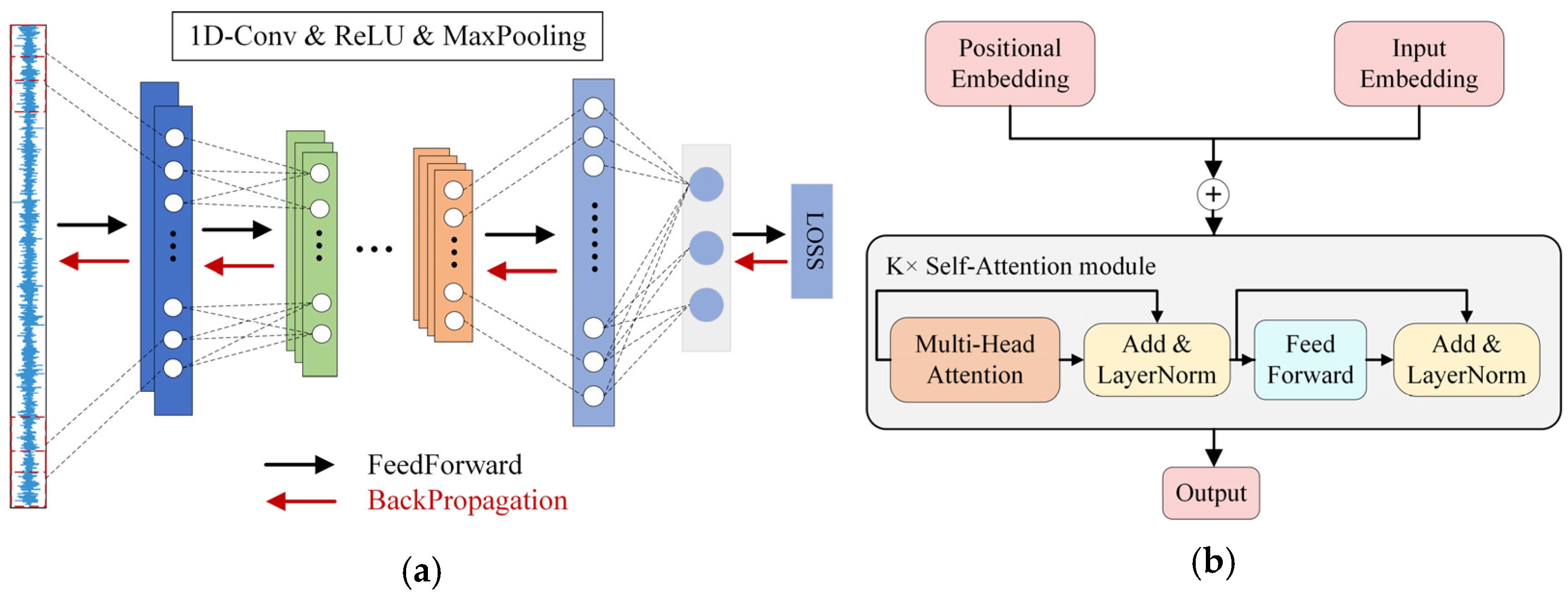[23] developed a new deep convolutional transfer learning network for intelligent fault diagnosis of machines with unlabeled data. Recently, various variants of 1D dimensional transformers have been proposed and achieved good performance in various tasks. Long-transformer [24] is an improved model with sparse attention to reduce computation cost and strengthen the ability of the long-distance encoder. Reformer [25] was designed with dot-product attention with locality-sensitive hashing attention, which effectively reduces time and memory costs. Universal transformer [26] was derived from transformer and RNN, which integrates the advantage of the global receptive field of transformer and the inductive bias of RNN. Transformer was firstly introduced into the image field by Vision transformer [27], which obtained good accuracy in image tasks.

Although excellent diagnosis performance has been obtained, most of the existing works rely on a large amount of labeled data and are trained centrally in a computing center. It is usually time-consuming and labor-intensive work. In the actual industrial environment, especially in aerospace applications, labeled data are usually independently owned by different institutions, and equipment is usually small-scale. How to combine the multiple datasets from different equipment to build a robust intelligent diagnosis model is still challenging work.

A natural idea is to integrate multiple datasets from different equipment to train a deep network model to form a shared large-scale dataset. However, there are two obstacles to practical application. Firstly, data migration out of the original storage centers causes data privacy leakage. In the information society, data have become a special resource for holders. Its characteristic is that once it is shared, its economic value is greatly reduced. Thus, many laws or regulations are created to prohibit data from being transmitted out of storage centers. Second, the data of different institutions are often collected in different working conditions or even different equipment; with a model trained on one condition, it is harder to obtain a strong generalization performance on other conditions due to the data distribution discrepancy.

For ensuring data privacy protection, federated learning provides a promising scheme. Federated learning allows multiple parties to jointly train a good network model and share the model results without revealing local original data. It not only meets the requirements of data privacy protection, but also obtains a model with better performance. Specifically, the participating parties, namely, clients, form a federation under the coordination of a trusted central server and cooperate to complete the entire process of model training [28]. The central server shares a pre-agreed network model with each client and the clients use the local dataset to execute several update steps on the received model through optimization methods. The model parameters are uploaded and distributed between the central server and clients in plaintext or encrypted until the model reaches the convergence condition. During the whole training process, there is only communication between the trusted central server and each participant, which avoids the risk of data privacy leakage to a certain extent.

Federated learning (FL), as an effective method, has attracted more and more attention in the industry. Some early applications of the federated learning techniques on intelligent fault diagnosis have been explored [29,30,31]. Zhang et al. [32] proposed a federated learning scheme based on self-supervision for bearing fault diagnosis. Zhang et al. [33] proposed a federated learning scheme using an adversarial transfer method for cross-working conditions. Chen et al. [34] designed a federated learning scheme with dynamic weighted aggregation of parameters to improve the classical federated average algorithm. In addition to the research on the global model, Yang et al. [35] proposed a personalized federated learning scheme based on averaging shared layers for diagnostic tasks, which allows clients to design classification modules according to their actual tasks.

However, there are three main challenges in FL applied to intelligent fault diagnosis. Firstly, most of the existing federated learning methods assume that the data of each client are collected from the same or different working conditions under the same equipment, so that the training data and test data come from the same distribution. However, different devices may be responsible for different products in manufacturing production lines and work under various operating conditions. Therefore, the data collected from different clients (devices) generally have different data distributions. If joint training is carried out directly, the diagnosis results are often not satisfactory. Secondly, the key to federated learning lies in the exchange of the encrypted weight or features among diagnosis models of different regions. However, existing federated learning schemes such as the federated averaging algorithm usually treat the encrypted features of each model equally, which ignores the differences of features in each model on the final diagnosis performance. Thirdly, A model structure that is adapted to the FL scenario is very important to ensure excellent performance. Existing deep learning-based models usually use convolutional structures to extract features, whose core mechanism is based on local receptive fields. This type of model pays more attention to local features while ignoring global and general features, which decreases the generalization performance of the model.

To solve the above problems, a CFL method based on a self-attention mechanism is proposed for bearing fault diagnosis across different device situations. The main innovations and contributions are as follows.

• Under the constraints of data privacy protection, a multi-client collaborative training solution named CFL is proposed for bearing fault diagnosis under different equipment, which effectively improves the existing FL method in the diagnosis field.
• To leverage the feature similarity and reduce the distribution discrepancy among different models, a k-means-based unsupervised cluster method is developed to learn common features from all participating clients, which integrates the data advantages of all clients and eliminates data distribution skew among different clients.
• A self-attention mechanism, rather than a convolutional structure, which can capture and directly extract the local and global features of the raw data, is designed for improving the accuracy and generalization performance of the model.

The remainder of this paper starts with related works in Section 2. The preliminaries are shown in Section 3. The proposed method is presented in Section 4 and the experiment result is presented in Section 5. In the end, the conclusion is arranged.

2. Analysis and Methods

2.1. Problem Description

This study focuses on federated learning for fault diagnosis of mechanical equipment with the following assumptions.

• A trusted central server coordinates the cooperation of each client for model training and the model is ultimately shared by all parties.
• The original data cannot be transmitted out of the local client, and information exchange between local clients is completed by the central server, which means there is no direct communication between local clients.
• Datasets held by multiple clients are collected from different machinery running under different working conditions. All parties hold a small amount of labeled data, and the data present a large distribution discrepancy.
• The diagnostic tasks of all clients are consistent and share the same model structure for training.

This can be summarized as follows: Assume the training data ${\mathrm{D}}_{train}={\left\{{(x_j^i,y_j^i)}_{j=1}^{ni}\right\}}_{i=1}^N$, where N represents that there are N clients totally and ni means that the client i owns ni training samples. Therefore, $(x_j^i,y_j^i)$ is one of the samples from the client i. During the training procedure, data from N clients are jointly used to train a model under the coordination of the central server. Correspondingly, the test set $D_{test}={\left\{{(x_k^i,y_k^i)}_{i=1}^{nk}\right\}}_{k=1}^M$ is used to evaluate the performance of the model. The final evaluation index of model performance is measured by the test set under M different test conditions.

2.2. Self-Attention Mechanism

The self-attention mechanism allows the model to directly utilize local and global features, resulting in better generalization performance than CNNs that rely on local features only. Much research denotes that using self-attention for model training can capture more general features of the data, which is more suitable for applications in various fields. A basic comparison of a CNN and a self-attention network is presented in Figure 1.

The CNN performs feature extraction in a sliding window manner through a convolution kernel shared by weights and obtains distributed feature representations by continuously stacking convolutional layers. The acquired high-dimensional features are used as the input of downstream tasks and the whole model is trained through the back-propagation algorithm. The network model, which is formed by stacking the basic blocks of convolution–activation–pooling, has information redundancy in the convolution operation and information loss in the pooling operation. These factors inevitably affect the generalization of the model performance.

By contrast, the model with the self-attention mechanism divides the input signal into small segments of equal length and uses them as basic signal elements to calculate the weights so that any segment of the basic signal can maintain the connection with the entire input signal. Specifically, the original signal is first divided into small segments of equal length and denoted as a token. The positional embedding information is added as alternative information for timing. It performs three sets of equal-dimensional linear transformations on each token to obtain three tokens, denoted as query, key, and value. Then, attention is implemented to each key for any query, and the attention result is normalized by the softmax layer, then multiplied by the value of the corresponding key as a new value.

The information loss is reduced by reconstructing the input signal through the attention mechanism so that the model can focus on more general features with significant correlation. In this way, the generalization performance of the model can be improved to a certain extent.

3. Proposed Clustering FL Method

3.1. Overview of The Proposed Method

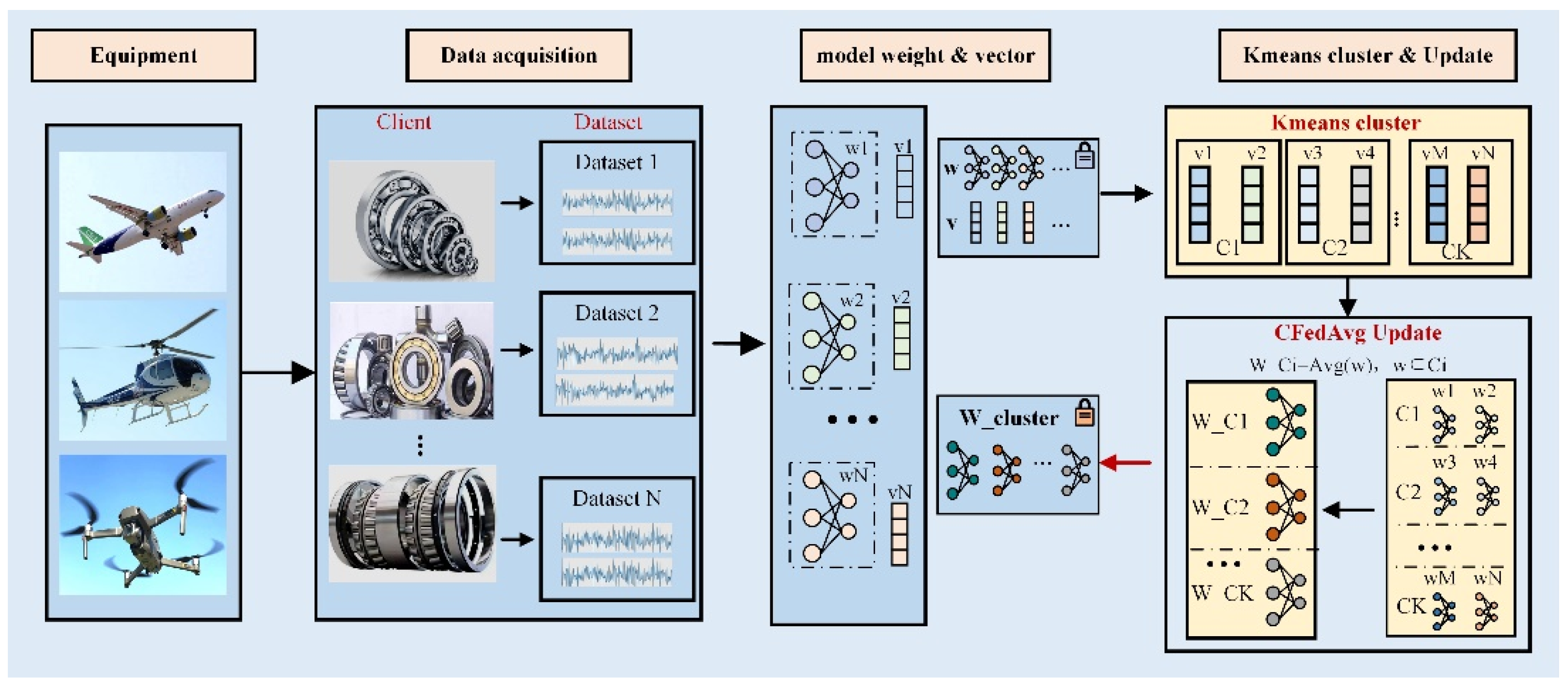
The overall flowchart of the proposed CFL is shown in Figure 2. Typically, the first and essential part is data acquisition, which use accelerators to collect vibration signals from different devices and build corresponding datasets. Then, the model can be designed with a deep neural network under the federated learning framework. In the model training stage, datasets from different clients are used to update the model parameters. Then, the updated results are sent to the central server. In addition, the server uses the KMeans cluster method to divide the clients into serval groups by the representation vectors, which further conduct a corresponding federated aggregation strategy to improve the learning performance under the data privacy condition. A detailed description of the proposed method is illustrated as follows.

3.2. Model Structure

The deep neural network structure designed with a self-attention mechanism is enhanced with a one-dimensional signal, which is named SiT in this paper. Its main structure is shown in Figure 3 and the main parameters are shown in

Table 1. Parameters of signal transformer.

Parameters	Value
Token size	4
Patch embedding size	64
Position embedding size	64
K blocks	2
MLP size	256

.

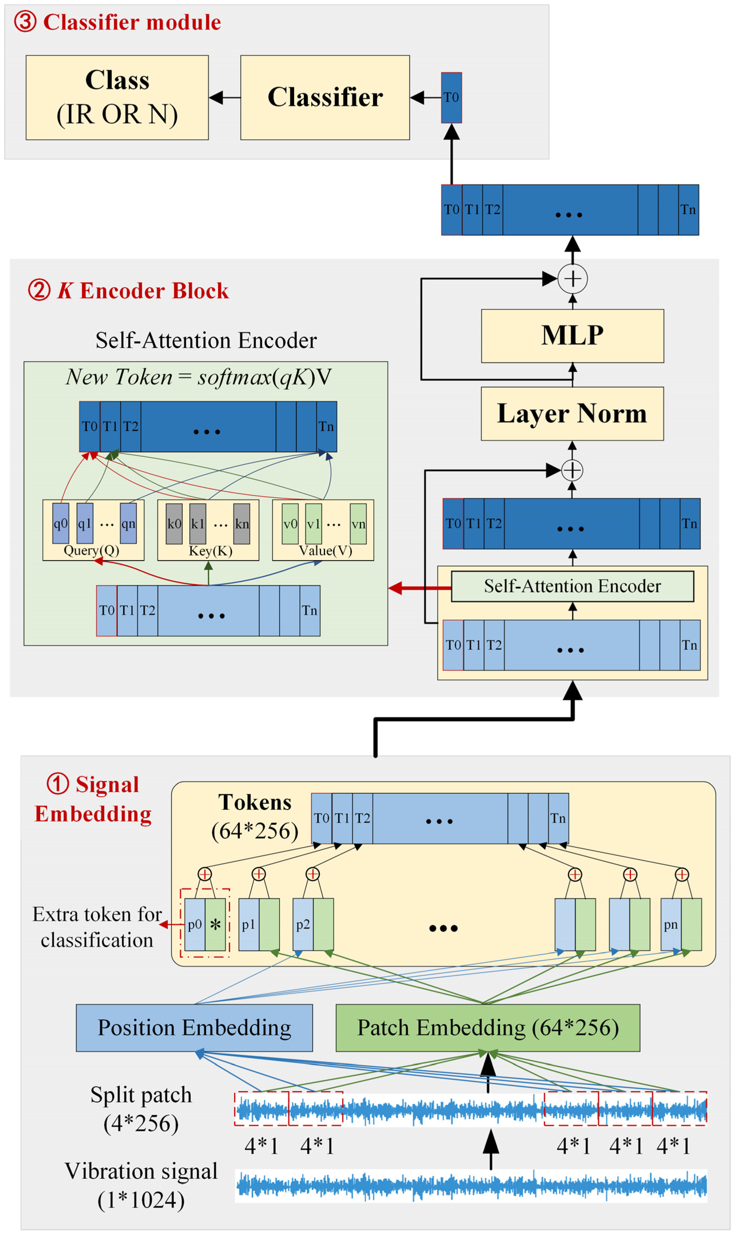
As shown in Figure 3, the model structure mainly contains three parts. The first is the signal-embedding part, which is composed of patch embedding and position embedding. The raw signal is firstly divided into small patches and transformed into high-dimensional vectors by the patch-embedding module, where 1*1024 denotes the input dimension of [1, 1024]. The position-embedding part is an independent module from the signal, which provides position information for the sequential signal. The output is a variable that has the same dimension as the patch embedding size. After patch embedding and position embedding, the outputs are added together into the next part.

After the first embedding process, raw signal data are transformed into a new form, namely, tokens, which is the addition of the patch embedding and position embedding results. Then, tokens are the input of the encoder part. The second part is the encoder block, which takes advantage of the self-attention mechanism. In detail, a token is transformed into a query, a key, and a value vector by three different transformation matrices. Then, the query and key vectors are used to calculate the attention score by the scaled dot-product computation, as shown in the self-attention module. After a softmax process, the new scores are the weight of the corresponding value vectors to obtain new tokens. The whole process can be represented as a formula.

$$Attention(Q,K,V)=softmax(\frac{Q{K}^{{\rm T}}}{\sqrt{d}})V$$

(1)

The encoder block also contains a residual connection layer, layer norm, etc., besides the self-attention module. All the details can be obtained in Figure 3.

The last part is a common classifier module. It is worth noting that the input of the classifier is not all the matrix, but just a slice of it. Usually, it is the zero position of the final feature map.

3.3. Model Pretraining

In the entire clustering federated learning method, the clients perform local model optimization and update steps. During the model optimization process performed by the clients, the local private dataset and classic optimization algorithm, i.e., stochastic gradient descent, are used to train the model. For labeling data, the optimization objective is to minimize the cross-entropy loss function, and the overall loss function of federated learning is defined as follows.

$$min{\displaystyle \sum _{i\in K}L(f_i(x);y)}$$

(2)

$$L={\displaystyle \sum _{c=1}^N-\frac{1}{nc}{\displaystyle \sum _{i=1}^{nc}{\displaystyle \sum _{k=1}^{K}I(y_i=k)\log \frac{e^{x_{i,k}}}{{\displaystyle \sum _{m=1}^K{e}^{x_{i,m}}}}}}}$$

(3)

where L represents the classification loss, N represents the number of clients and represents the total number of samples of client C. At the same time, it can be seen from Figure 2 that the high-dimensional features obtained by the feature extraction module through the backbone network are in the shape of 1*64. This means a sample can be compressed into a 64-dimensional vector. The same operation is performed on all the samples to obtain a sample size * 64 matrices; then, further compression in the sample dimension is executed to obtain a 64-dimensional vector, which is used as the data distribution representation vector of this client. Finally, the representation vector, together with the optimized model weights, are uploaded to the central server.

3.4. K-Means Cluster in CFL

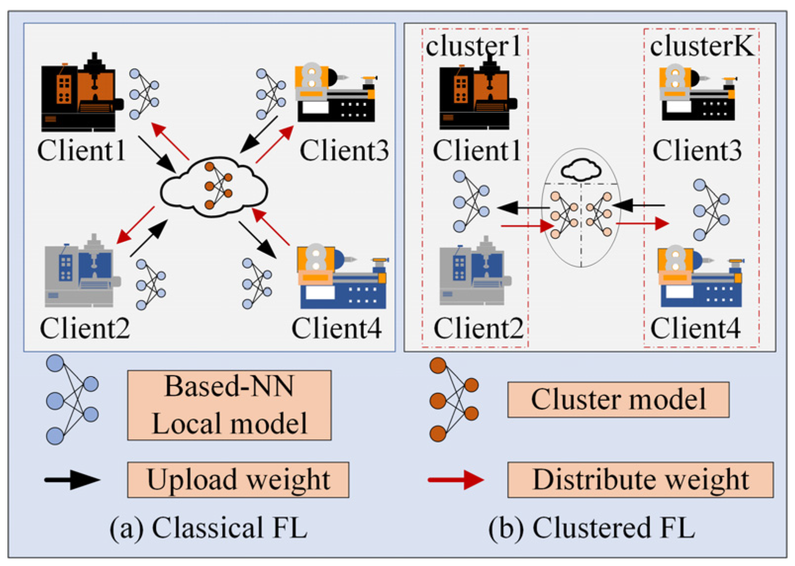
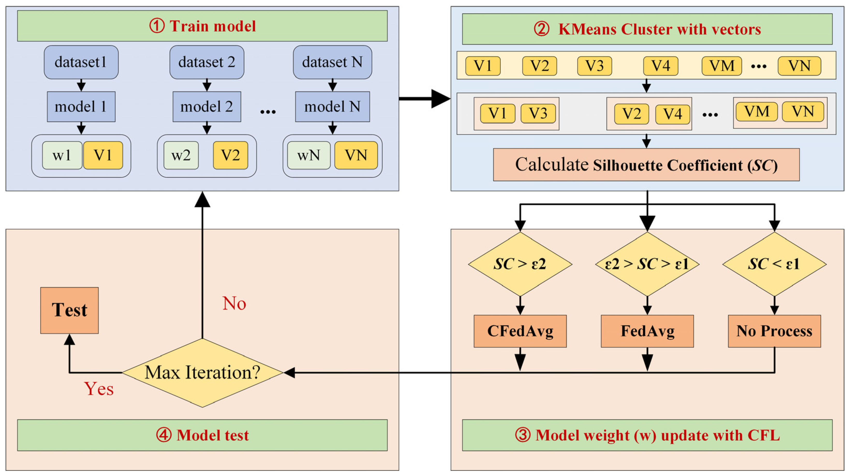
Unlike the classical federated learning algorithm, which directly implements the weighted average obtained from the models in all the clients (devices), the proposed federated learning strategy first implements the device clusters based on the feature similarity among different models in each client. Then, the features from similar groups are implemented with the federated average algorithm, as shown in Figure 4.

Since the k-means, as the typical unsupervised clustering method, can classify the clients with high similarity into the same cluster and those with low similarity into different clusters, it is used to cluster the clients with similar data distribution into the same cluster, and then perform federated learning training within the cluster. The clustering algorithm and the federated aggregation are executed sequentially. The clustering results are adjusted iteratively until they converge to the desired effect.

During the clustering procedure, the features are extracted from self-attention mechanism, which further extracted the statistical average information along each channel as the input of k-means clustering. It not only reduces the additional calculation amount, but also avoids possible data privacy leakage. Then, the unsupervised clustering is further implemented to determine the similarity of clients, which can not only effectively utilize data resources with high similarity, but also reduce the impact of data distribution discrepancy on model performance.

Specifically, after the server receives the statistical average representation vectors and model weights are uploaded by the clients, an unsupervised clustering algorithm is performed first to divide the clients into different cluster groups with similar data distribution. In the proposed scenario, since there are not many categories and the data dimension is not high, a k-means clustering algorithm with the specified number of clusters is directly used. The objective optimization function is as follows:

$$J(c,\mu )={\displaystyle \sum _{i=1}^K\left|\right|x_i-{\mu }_{ci}|{|}^2}$$

(4)

where $x_i$ is the i-th vector, $c_i$ is the cluster that $x_i$ is resigned. ${\mu }_{ci}$ represents the center of the cluster and K is the number of vectors. During the implementation procedure, it should select the cluster centroid with the closest distance to the vector and repeat the above optimization process until the above formula converges for any data point. After the clustering is completed, the clustering results are analyzed. The silhouette coefficient, named SC, is selected as the evaluation clustering index. The formula for calculating the contour coefficient is listed as follows.

$$SC=\frac{1}{K}{\displaystyle \sum _{i=1}^K\frac{b(x^{(i)})-a(x^{(i)})}{\max \{a(x^{(i)}),b(x^{(i)})\}}}$$

(5)

where $x^{(i)}$ is one of the vectors for clustering, $a(x^{(i)})$ is the average distance between $x^{(i)}$ and others in the same cluster, and $b(x^{(i)})$ is the minimum distance between $x^{(i)}$ and others in the different clusters. K is the total number of clusters. SC is the average value of the sum of all vectors. The value of SC is between −1 and 1. What is more, the closer SC is to 1, the better the clustering performance will be. After the central server executes the clustering algorithm, it selects the corresponding federated aggregation strategy according to the confidence of the clustering effect.

We can take advantage of the SC value to build the update strategy. For example, $\epsilon 1$ and $\epsilon 2$ are adopted to represent the two thresholds of the silhouette coefficient $(-1\le \epsilon 1\le \epsilon 2\le 1)$.

Generally, if the contour coefficient of the clustering result is greater than the threshold $\epsilon 1$, it means that the clustering performance of the current round is ideal and the similarity between clusters is small; then, the model weights are clustered according to the clustering results. The aggregation formula is given as follows.

$${\mathrm{w}}_{gk}=Avg({\displaystyle \sum _{c\in k}{w}_c)}$$

(6)

where W_gk represents the averaging weights of clients belonging to k-th cluster. Then, W_gk is sent to the corresponding clients to optimize the parameter of each model.

If the contour coefficient of the clustering result is less than the threshold $\epsilon 2$, it means that the clustering effect of the current round is relatively poor, and the similarity between clusters is large. Then, the server does not process the weights of the models in this round. If the silhouette coefficient is between $\epsilon 1$ and $\epsilon 2$, then a global federated averaging update is performed.

$${\mathrm{w}}_g=Avg({\displaystyle \sum _{c\in all}{w}_c)}$$

(7)

Usually, the threshold should be carefully designed to control the weight of clustering federated learning. In the proposed method, $\epsilon 1$ and $\epsilon 2$ are two significant factors in the performance of federated learning, which should be carefully selected to control the weight of clustering federated learning. In this study, the grid-search method, as a widely adopted technique, is adopted to determine the value of $\epsilon 1$ and $\epsilon 2$. To be specific, $\epsilon 1$ and $\epsilon 2$ are set in the range of −1 to 1, and $\epsilon 2$ should be larger than $\epsilon 1$ to construct a suitable bound. When $\epsilon 1$ is large, it is more inclined to perform a local update and when the value is small, it is inclined to adopt federated averaging updates. When $\epsilon 2$ is small, it prefers to use a clustered federation update, while if the value is large, it prefers to use a global federation update. Finally, $\epsilon 1$ is set at 0.5 and $\epsilon 2$ is set at 0.8 by a grid search among the restricted hyper-parameter ranges. With such a general clustering federated learning strategy, the constructed fault diagnosis model can be well trained under the data privacy preservation framework.

3.5. Flowchart and Algorithm of CFL

The flowchart of the entire CFL is presented in Figure 5. The specific steps are as follows. Furthermore, algorithm 1 shows the pseudocode of the proposed method.

Step 1: The server initializes the model parameters and sends them to the clients.

Step 2: The client uses local data to optimize the model and uploads the model weights and data representation vector to the server.

Step 3: The server first uses the client’s representation vectors to perform unsupervised clustering of k-means to gather clients with similar data distributions into the same cluster. Then, the corresponding federated update strategy is decided and performed according to the clustering performance.

Step 4: The server sends the weight obtained by the aggregation process to the corresponding clients, which is used for updating the independent model in each client.

Step 5: Repeat steps 3–5 until the model stop condition is reached.

4. Experimental Results

4.1. Dataset Description

To validate the effectiveness of the proposed fault diagnosis method under the FL framework, there are three bearing datasets adopted which can be used in aerospace applications. The first one, named the CNC bearing dataset, is collected from a CNC milling machine operated at different speeds. The other two datasets are the public testbed bearing datasets, i.e., the Machinery Failure Prevention Technology (MFPT) bearing dataset [36] and the Paderborn University bearing dataset [37].

CNC machining services are highly essential in the aerospace sector. It is a manufacturing process that uses a combination of high-speed rotation and cutting tools to remove material from a solid workpiece. The failure of bearings in CNC has a big effect on the reliability of high-quality aerospace parts. The CNC dataset is collected from a rotary spindle of a CNC machine, which was used for cutting aluminum and steel materials in aerospace applications. The speed condition covers from 6000 rpm to 10,000 rpm. The data are collected with vibration sensors and the sampling frequency is 25 kHz.

The MFPT bearing dataset comprises data from a bearing test rig (nominal bearing data, an outer race fault at various loads, and inner race fault and various loads). Furthermore, the vibration signals are acquired. The test rig in the MFPT can be used for simulating the failure of bearings of the transmission system in aerospace applications. The sampling frequency for the normal state is 97,656 Hz and 48,828 Hz for the fault state, respectively.

Similar to the MFPT bearing dataset, the Paderborn bearing dataset is constructed for simulating the failure of bearings in aviation systems under different operation conditions. This bearing dataset is provided by the Chair of Design and Drive Technology, Paderborn University. It is collected in the test bench under different rotational speeds, torques, and radial force conditions, where three kinds of health statuses, including inner race fault (IR), outer race fault (OR), and normal state (N), are obtained. The sampling frequency is 64 kHz and the vibration signals are obtained with vibration sensors. A detailed description is shown in

Table 2. Description of the three datasets.

Dataset	CNC	MFPT	Paderborn
Health condition	IR, OR, N	IR, OR, N	IR, OR, N
Rotate speed (rpm)	6000, 7000, 8000 9000, 10,000	1500	900, 1500
Load	0	0	0.1, 0.7 (Nm)
Radial force	0	25, 50, 100, 150, 200, 250, 280, 300 (lbs)	400, 1000 (N)
Static load rating (N)	7950	/	4750
Dynamic load rating (N)	106,000	/	9500

.

The measurements collected in the three considered datasets are all vibration signals. Naturally, the data forms are homogeneous. As shown in Table 2, we can see that health condition contains three states, that is, inner fault (IR), outer fault (OR), and normal (N), in the three considered datasets. Rotate speed is the rotation speed of the shaft and load represents a moment acting on the shaft, while radial force is a force acting on the bearing in the radial direction.

As shown in Table 2, we can see that health condition contains three states, that is, inner fault (IR), outer fault (OR), and normal (N), in the three considered datasets. Rotate speed is the rotation speed of the shaft, and load represents a moment acting on the shaft, while radial force is a force acting on the bearing in the radial direction.

It is worth noting that 0 means the load is an operation in a no-load condition or the applied radial force is 0 in Table 2. This means that the machine is working in an idle state, which is a normal state. It should also be noted that for the three different datasets, there are 30 samples available for model training in each class under each condition. Each sample has a length of 1024 data points. In addition, there are 150 samples available in each class under each condition for the final testing.

According to the actual situation, the equipment of different clients may be different and the operating conditions of the equipment also vary with the change in the manufacturing products. Naturally, the datasets constructed from the same machinery under different operation conditions or similar machinery follow different distributions. Without loss of generality, different datasets under eight working conditions are designed as the corresponding clients for experimental validation. The experimental setup is detailed in

Table 3. Client dataset and test task description.

Client	Dataset	Working Condition
Client 1	CNC	6000 rpm
Client 2	CNC	7000 rpm
Client 3	CNC	8000 rpm
Client 4	CNC	9000 rpm
Client 5	CNC	10,000 rpm
Client 6	MFPT	25 lbs
Client 7	MFPT	50 lbs
Client 8	MFPT	150 lbs
Client 9	Paderborn	N15_M01_F10
Client 10	Paderborn	N09_M07_F10
Client 11	Paderborn	N15_M07_F10
Client 12	Paderborn	N15_M07_F04

.

4.2. Comparison Methods

To demonstrate the advantage of the proposed method, three different methods, namely, local update (Baseline), Federated Averaging (FedAvg), and FedProx, are adopted for algorithm comparison.

Baseline: For the baseline method, only local data are involved in model training and the trained model is tested on testing data. It corresponds to the extreme case of the proposed method where the number of cluster centers is equal to the number of clients.

FedAvg: As a classic federated learning algorithm, the federated averaging algorithm has always been an essential criterion for baseline comparison. For FedAvg, the weights of each local model are firstly averagely aggregated to obtain the total weights, which are further downloaded into the local model for the updated weight. It corresponds to the extreme case of the proposed method where the cluster center is equal to 1. Some research-related FedAvg algorithms have been developed in the fault diagnosis field, such as enhanced weight aggregation and federated transfer learning.

FedProx: As an improved method of federated averaging learning, FedProx reconstructs the local optimization goal, which is the combination of the empirical risk of the local dataset and the regularization term of the global model and the local model in each iteration process. It aims to force the client model intending to the global model so as to accelerate model convergence and improve accuracy.

The experimental settings in all the comparison algorithms are shown in

Table 4. Experimental setup parameters.

Parameter	Value
Global iteration	50
Local iteration	5
Sample length	1024
Batch size	8
Learning rate	0.001
Optimization	Adam

.

4.3. Experimental Results

4.3.1. Effectiveness of the Constructed Self-Attention Model

Firstly, an experiment is conducted for comparing the performance of different advanced networks. In this study, the considered networks contain RNN, LSTM [3,4], 1D-CNN [5], and the constructed self-attention module (named SiT). For a fair comparison, the difference among all the networks is the backbone module, which is used for feature extraction, and the classifier modules are the same. In detail, the raw vibration signals are taken as the input of all networks and the dimension is 1*1024. RNN and LSTM have two layers and the hidden size is 128. 1D-CNN has one convolutional module, where the kernel size is 64 and the stride is 16. Furthermore, there is only one self-attention block in SiT, where the main parameters are similar to Table 1 and the number of blocks is only one. After the feature extraction process with the backbone module and a ravel operation, the raw signal is encoded into a vector, whose dimension is 1*128. Then, the feature vectors are sent into a classifier module, which is composed of two fully connected layers, whose hidden units are 128 and 3.

What is more, the number of experimental samples is 20 per class and the experimental results are listed in

Table 5. Performance comparison of different networks.

	Client 2	Client 3	Client 4	Client 5
RNN	40.77 ± 3.17	60.62 ± 1.34	40.02 ± 7.51	45.08 ± 1.11
LSTM	66.1 ± 8.17	69.2 ± 6.4	78.2 ± 10.89	64.95 ± 13.2
1D-CNN	90.9 ± 0.13	88.37 ± 1.34	89.25 ± 0.05	86.93 ± 5.42
SiT	100 ± 0	100 ± 0	99.08 ± 0.03	99.93 ± 0.08

.

As shown in Table 5, RNN and LSTM are not good at handling vibration signals, because the signal is too long to be processed well. 1D-CNN has a better performance for vibration signals. Compared with the three networks, the proposed SiT has the best performance in all clients.

As shown in Table 5, both RNN and LSTM achieve low testing accuracy, as the signal is too long to be processed well, while 1D-CNN has a better performance than the above methods due to its advantages of handing vibration signals. By contrast, the proposed SiT has the best performance in all clients, which demonstrates its superiority in feature extraction and fault classification.

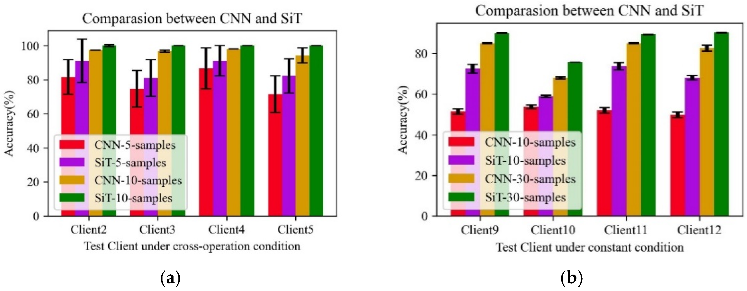
What is more, to further evaluate the performance of the proposed method, two further experiments were conducted to verify the superiority of SiT. Two different experimental datasets including the same operating conditions and cross-operation conditions have been designed.

In the constant operation condition experiment, the data from Client 9, Client 10, Client 11, and Client 12 are selected. Different training samples with 10 and 30 in each class are adopted for training the model, while the rest of the samples are utilized for testing. The experimental results are shown in Figure 6a. Under cross-operation conditions, data from Client 1 are used as training data, and data from Client 2, Client 3, Client 4, and Client 5 are used as test data. In the experiment, the number of 5 and 10 samples in each class is adopted for training the model, respectively, while the rest are for testing. The experimental results with different sample numbers are shown in Figure 6b.

It can be seen from the results that the proposed SiT is much better than that of the CNN under the same working conditions. With the availability of the limited 10 samples, the CNN only achieves below 60% accuracy, while the proposed method is much higher in most of cases. What is more, with the increase in the number of samples, the accuracy of the CNN is raised, but is still lower than the proposed SiT. Under the cross-working conditions, similar results can be found among all the cases, which indicates that the proposed SiT has better performance. The better performance achieved is possibly due to the advantages of the constructed self-attention mechanism in capturing the local and global features from the input samples. As such, the learned features are much more robust than that of the CNN, especially in the case of the limited samples.

4.3.2. Experiment Results among Different Methods

In real industrial applications, the monitoring data may come from different devices under different operation conditions. However, the limited data cannot meet the training of a robust decision model. Thus, it is expected that similar mechanical data scattered across different areas can be effectively combined to leverage its potential and business value under the federated learning framework. In this experiment, three federated learning-based fault diagnosis tasks (task1, task2, and task3) were designed, as shown in Table 1. In the constructed tasks, the mechanical data from Client 1, Client 2, Client 3, Client 4, Client 6, Client 7, Client 9, Client 10, and Client 11 are adopted for training. For each client, there are only 10 training samples in each class available, while the data from Client 5, Client 8, and Client 12 are adopted for testing. It can be seen that the training data cover different operation conditions and three different machinery equipment. They also follow the different data distribution due to the variation of the working environment. It should be noted that data from different clients are separately utilized to train its independent model to carry out its diagnosis task without direct contact with each other at the data level. Thus, each task attempts to make use of the additional mechanical data from different clients to improve its diagnosis performance under the condition of the limited available data.

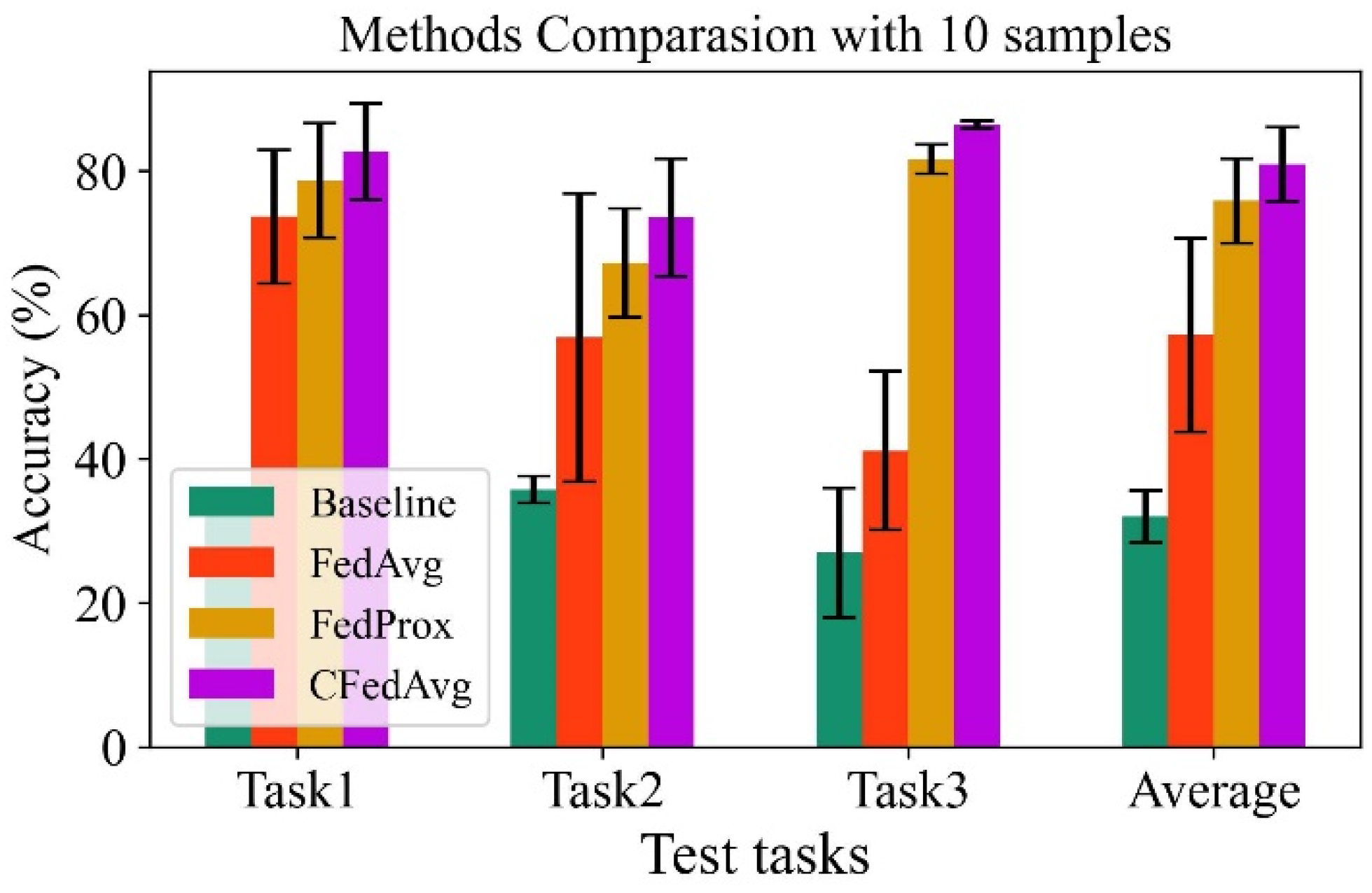
To validate the effectiveness and superiority of the proposed method (CFL), which is implemented as CFedAvg, three existing techniques, including Baseline, FedAvg, and FedProx methods, are adopted for performance a comparison. A total of five repetitive experiments are conducted and the average results, including the testing accuracy and standard deviations, are presented in Figure 7.

It can be seen that the worst diagnosis performance is obtained in the Baseline method, where there is below 40% testing accuracy in each test task. This is because the learning ability of a deep neural network should be activated by sufficient training data. In the Baseline method, there are only ten samples in each class adopted for the training, which is not enough for training a robust diagnosis model. For the FedAvg and FedProx, it is expected that obvious improvement on accuracy can be found in each task in comparison with the Baseline method, since multiple different bearing datasets from different clients are jointly used in the federated learning framework. The learned diagnosis knowledge from different models can be utilized with the weight average algorithms. Thus, the learning ability of the model in each Client trained with limited training data can be enhanced by the global weight share strategy obtained through the combination of the weight in each client. In particular, the proposed CFL method obtains an excellent diagnosis performance which is superior to all the other methods. The advantages lie in the use of the constructed federated cluster learning strategy, which not only effectively reduces the negative effects caused by data distribution shifts, but also uses the data resources of similar clients to improve model performance.

4.3.3. Parameter Effect of the Number of the Cluster

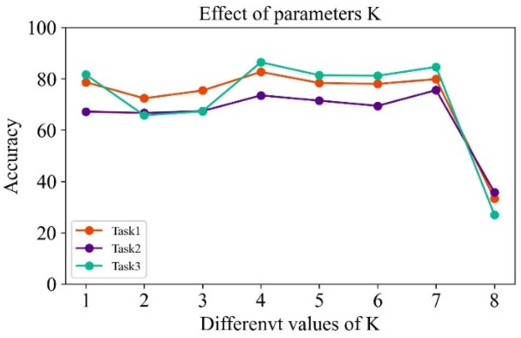
During the model training procedure, it is important to select the suitable parameter of the number of cluster K, which directly determines the different federated clustering strategy. In this experiment, since the maximum number of clients is eight (representing eight different training datasets), the number of the clusters are changed from 1 to 8 to investigate its effect on the final diagnosis performance. It should be noted that when the number of cluster K is equal to 1, it corresponds to the global federated averaging algorithm (FedAvg), and when K equals 8, it corresponds to the Baseline method, where no federated learning strategy is implemented. The effect of different values of k on model performance is presented in Figure 8.

It can be seen that when K equals 1, it corresponds to the FedAvg method, which achieves high diagnostic accuracy in all three tasks. This is because each model in the client could leverage the diagnosis knowledge from other clients by implementing the federated average algorithm. When K is equal to 4, the diagnostic accuracy is improved; the improvement is nearly 20% for task 2. When only using local data for training (K = 8), the model achieves the lowest test accuracy on the three tasks. This is consistent with the results of the Baseline method obtained in Figure 7 due to the limitation of the small sample sizes and lack of data utilization from other clients.

Furthermore, different values of K have different influences on the final testing accuracy. Choosing the appropriate K value plays a crucial role in the whole model training. When the K value reaches 4, it obtains the best performance, which is selected as the optimal parameter.

4.3.4. Feature Visualization with Quantitative and Qualitative Analysis

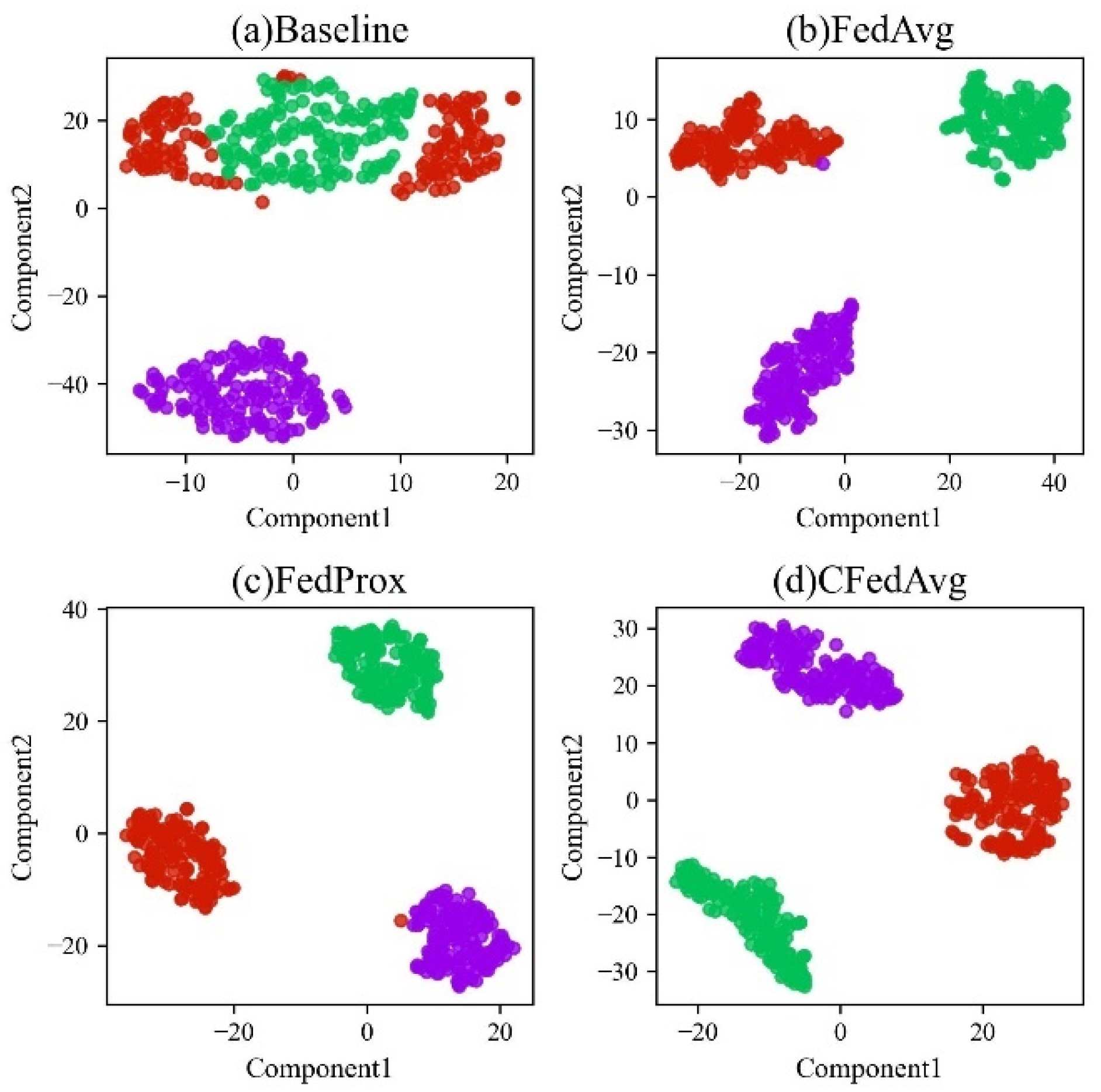
To better estimate the learning performance of the extracted features among different methods, taking the diagnosis task T1 as an example, the learned high-dimensional data representations in the fully connected layers are adopted. They are further reduced into 2-D features for feature visualization to provide a better understanding of the discriminability by using the typical t-SNE technique.

The results are presented in Figure 9, where different colors denote different health conditions. It can be seen that the Baseline performs worst among all the methods. The sample points corresponding to class 2 scatter into two different regions, indicating that they follow two different feature distributions. It can be expected that the learned feature cannot meet strong generalization performance and the diagnosis accuracy is poor, which is consistent with the result in Figure 2. While the other two federated learning-based diagnosis methods are all superior to the Baseline method, the sample points from the same classes can cluster well and those from different categories can be easily distinguished, which contributes to obtaining better diagnosis accuracy.

However, from the intuitive visualization results, it is still difficult to judge which models are better for learning strong discriminative features. Furthermore, quantitative analysis indexes, named the intra-class and inter-class correlations, are further constructed to evaluate the learned high-dimensional features of the test dataset. Specifically, two parametric metrics are used: between-class covariance and within-class covariance. Among them, the high-dimensional feature matrix of the test set samples is:

$$f=[f_1,f_2,\dots ,f_N]$$

where f_i denotes the extracted features in the i-th samples. Then, the between-class covariance and the within-class covariance are defined as:

$$S_b={\displaystyle \sum _{c=1}^K{N}_c(m_c-m){(m_c-m)}^{\mathrm{T}}}$$

(8)

$$S_w={\displaystyle \sum _{c=1}^K{\displaystyle \sum _{n\in c}(f_n-m_c)(f_n}-m_c{)}^{\mathrm{T}}}$$

(9)

where $N_c$ is the total number of class c, $m_c$ refers to the mean value of features in the class c of all K classes, and m is the total mean value of all the features. $S_b$ is the inter-class covariance and $S_w$ is the between-class covariance. If $S_b$ is bigger, the more dispersed the different classes are. The smaller $S_w$ is, the more concentrated the samples within the class are. The relationship between $S_b$ and $S_w$ is used to define four indicators to characterize the classification performance.

$$J1={\mathrm{Tr}[\mathrm{S}}_w^{-1}{\mathrm{S}}_b]$$

(10)

$$J2=\frac{\left|S_b\right|}{\left|S_w\right|}$$

(11)

$$J3=\frac{{\mathrm{Tr}[\mathrm{S}}_b]}{{\mathrm{Tr}[\mathrm{S}}_w]}$$

(12)

$$J4=\frac{|S_w+S_b|}{\left|S_w\right|}$$

(13)

Though the forms of J1, J2, J3, and J4 are different, they have a similar meaning to evaluate the classification manner. Generally speaking, if the value of J is larger, the performance of the model is better.

The qualitative analysis of the extracted features among different methods is presented in

Table 6. Quantitative analysis of J.

	J1	J2	J3	J4
Baseline	404.9	14.6	11.0	15.5
FedAvg	431.6	7.5	6.2	8.2
FedProx	248.3	1.9	1.9	2.6
CFedAvg	621.1	19.7	15.4	20.2

. It can be seen that the proposed method achieves obviously better learning performance among all the compared methods based on evaluation indexes. The excellent clustering ability of the extracted features further demonstrates the effectiveness and superiority of the proposed method, which provides an effective solution for the machinery fault diagnosis under the data privacy preservation condition.

5. Conclusions

Under the limited available samples and data privacy requirement, a novel CFL method integrating a self-attention mechanism and a clustering federated learning strategy is proposed for the intelligent fault diagnosis of bearings in aerospace applications. At the network level, a network model based on a self-attention mechanism is constructed to replace the traditional CNN model, which can directly utilize global and local features for model learning to improve the generalization performance. At the federated learning level, an enhanced k-means-based federated learning strategy is proposed based on client data distribution similarity, which improves the performance of the model effectively. The proposed approach has been fully validated by bearing datasets from different equipment in aviation systems under different operation conditions. The effectiveness and superiority have been fully validated in comparison with other methods, which provides an effective learning scheme for intelligent fault diagnosis under the data privacy preservation framework.

Although good performance has been achieved, it should be noted that the client data distribution representation vector in the proposed method is determined in the form of a data statistic, and there may be a certain deviation in practice. In the future, we will consider designing a representation method for adaptively learning the local data feature distribution to accurately characterize client data distribution. In addition, there is a certain deviation in the theory of specifying the number of clusters in advance, which has a certain degree of influence on the performance of the model, which will be further studied in following work.