
Numerical Analysis on the Aerodynamic Characteristics of an X-wing Flapping Vehicle with Various Tails


School of Aeronautic Science and Engineering, Beihang University, Beijing 100191, China
*
Author to whom correspondence should be addressed.
Aerospace 2022, 9(8), 440; https://doi.org/10.3390/aerospace9080440
Submission received: 5 July 2022
/
Revised: 9 August 2022
/
Accepted: 9 August 2022
/
Published: 11 August 2022
(This article belongs to the Special Issue Advances in Aerospace Sciences and Technology III)
Abstract
:X-shaped flapping wings have excellent maneuverability and flight capabilities under low-Reynolds-number conditions. An appropriate tail can extend the range of a vehicle and improve its stability. This study takes two typical configurations, the inverted T-tail and the inverted V-tail, as the research object. Considering the wings’ flexible deformation in the flapping process, the computational fluid dynamics method was used to calculate the vehicles’ aerodynamic characteristics, taking into account the aerodynamic interaction effect of the wings and tail. The results show that the wake of flapping wings can significantly reduce the forward flight performance of the tails. The maximum L/D ratio of the two tails decreased by about 38%, and the static stability was also dramatically reduced in the forward flight. The inverted V-tail has better performance in fast forward flight, while the inverted T-tail had better control characteristics at low speeds. The relationship between the tail layouts and aerodynamic performance is also discussed. When the inverted V-tail is in the optimal position, the longitudinal control moment can be doubled in the hovering state. This research provides a reference for the design and arrangement of flapping wings with tails, which is beneficial to the performance improvement of vehicles.
1. Introduction
Flapping wing micro aerial vehicles (FMAVs) are a kind of aircraft designed according to the bionics principle. They have been applied increasingly widely in military and civilian fields owing to their excellent characteristics, such as small size, low noise, and high flight efficiency under low Reynolds numbers. According to the layouts of FMAVs, biological flapping wings can be divided into two types: vehicles directly imitating flying-animal shapes and motions, including insect-like FMAVs, bird-like FMAVs, bat-like FMAVs, and vehicles based on bionics-inspired innovation, such as flapping rotary wings [1,2] and X-shaped biplane flapping wings [3].
Recently, X-shaped flapping wings have attracted increasing attention from researchers [4,5] due to their high propulsion efficiency, stable flight trajectory [6], hovering ability, and strong maneuverability. The dynamic and control characteristics of flapping wings are the focus of our attention in this article. Although there are some methods by which to control the attitude of the vehicle, such as by changing the asymmetrical aerodynamic force of the flapping wings [7,8,9,10], it is often necessary to add additional control mechanisms and weight. Due to the weight constraints of flapping-wing aircraft being relatively strict, an increased weight often limits the flight performance of the vehicle, such as flight range and time. The DelFly Nimble uses a torque coupling servo to achieve high agility in tailless layouts. However, the hover duration is reduced by 55% as compared to the DelFly II;.
At present, attitude stability and control of X-shaped flapping wings are mainly achieved by deflecting the tail control surface, the same as occurs with fixed-wing aircraft [11]. This is a mature and stable way to control the attitude adjustment and trajectory change of the flapping wing, by the deflection of the tail-control surface. A good design of the tail can not only enhance the static stable margin and control the characteristics of the flapping wing but can also reduce wake effects or even make full use of the vortex energy to improve the flight performance. Therefore, it is important to have a detailed tail design for flapping-wing vehicles.
However, in current tail designs, the influence of the flapping wake on the control effect of the tail is rarely considered. When examining tail design, Grauer [12] used the wind-tunnel test method to measure the tail control effect at different forward velocities and attack angles in steady states. The interaction between the wings and tail were not considered in the dynamic modeling.
To date, there have been some studies on the aerodynamic interaction between wings and tails. The majority used the CFD method to study the two-dimensional flapping-tail interference. Tay [13] used the immersed boundary method to study the wing-tail effect of a two-dimensional X-shaped biplane flapping wing. Their study showed that a horizontal tail can improve both the thrust and aerodynamic efficiency of the vehicle. Compared with a single flapping wing, the overall efficiency and the average thrust of each wing was increased by 17% and 126%, respectively, under the appropriate arrangement of the tail position and setting angle. Wang [14] used the dynamic mesh method to analyze the influence of reduced frequency on the thrust coefficient. The results showed that reduced frequency was the key parameter affecting the thrust. A higher reduced frequency strengthens the vortex shedding and results in an increase in the thrust coefficient. Deng [15] calculated the unsteady aerodynamic force of the X-wing using CFD simulation by employing the overset method and showed the vortex structures during the flapping process. Yang’s [16] research showed that the pitching and plunging motion of flapping wings can increase the maximum lift coefficient and stall angle of the horizontal tail, as compared with the steady state. However, due to the limitations of a two-dimensional numerical simulation, there were some differences between the results and the actual flow.
Some researchers have also studied the aerodynamic interference mechanism of the three-dimensional flapping-tail interference using the particle tracing method. By using the PIV method, Percin [17] analyzed the complete wake topology and evolution of this specific X-shaped MAV in forward-flight conditions in detail, but experiments using the particle tracking method were unable to quantitatively study the interference degree, as the experiment preparation processes were cumbersome. In addition, due to the extremely small size and light weight of the flapping wings, the experiments for the measurement of the force on the tails inevitably introduces other large disturbances.
In this study, considering the flexible deformation of the wings, the CFD method was used to analyze the three-dimensional-wings–tail interference of the X-shaped flapping wing. This article compares the aerodynamic characteristics of the conventional inverted T-tail and the inverted V-tail that represent two types of tails. On the one hand, the height of the tails relative to the wings are different. The inverted T-tail is located above the axis of the fuselage, while the inverted V-tail is located below. On the other hand, the inverted T-tail is composed of two faces at right angles to each other, while the V-tail is composed of two faces that are slanted. The surface composition represents a different wetted area and weight under the same projected area.
This article is organized as follows: based on the high-precision CFD simulation method, we studied the law of aerodynamic interference between the wings and two types of tails of the X-shaped flapping wing. The following section introduces the research model and proposes a simplified flexible wing motion based on the experimental results. In the third section, the aerodynamic characteristics of the X-wing vehicle with different tails are analyzed according to the simulation results. Then, the effect of tail position and dihedral angle are discussed. The microscopic mechanism of the flow is analyzed to explain the flapping influence on different tails. The final section summarizes this article.
2. Numerical Simulation Method
2.1. Reference Experimental Setup
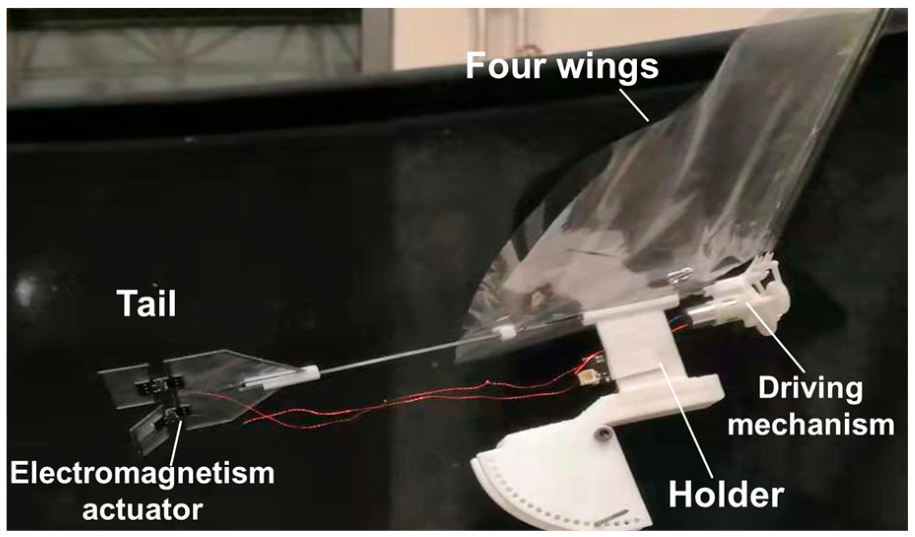
The reference experimental setup is shown in Figure 1. The wings were made of polyethylene material, and the surface thickness is approximately negligible. The roots of the wings were fixed on the carbon-fiber fuselage, so the distance between root of upper-wing and root of bottom-wing was quite close in the process of flapping.
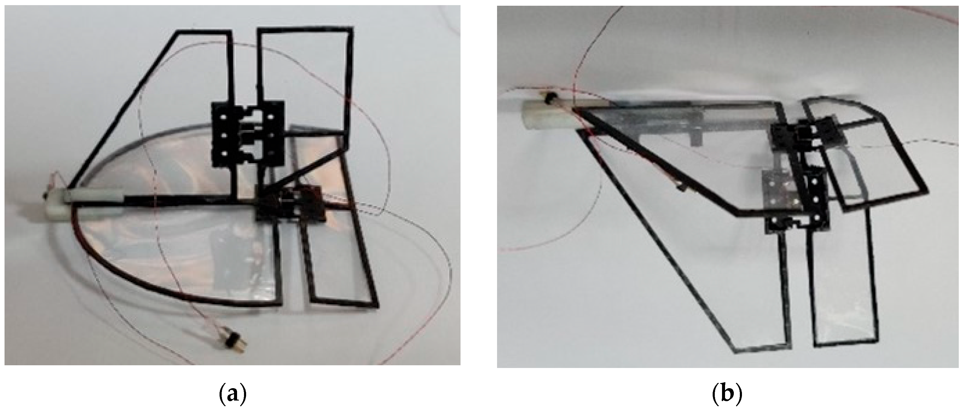
For the research object of this study, we selected the conventional inverted T-tail and inverted V-tail of the flapping wing, as shown in Figure 2. The inverted T-tail has better performance in the hovering state and the process of take-off and landing. An inverted V-tail can produce a positive lateral-directional coupling effect, which is beneficial for improving the maneuverability of flapping wings [18]. The tail control surfaces used electromagnetic actuators, which can be quickly deflected at the degree of 0 and ±45.
2.2. Model Parameters
2.2.1. Wings Model
2.2.2. Tail Models
In Section 3.1, the force and control characteristics of the two are compared under the condition of the same projected area of the stabilizer and control surface. The projection area of the control surfaces is also the same. The parameters of the two tails are shown in Table 2.
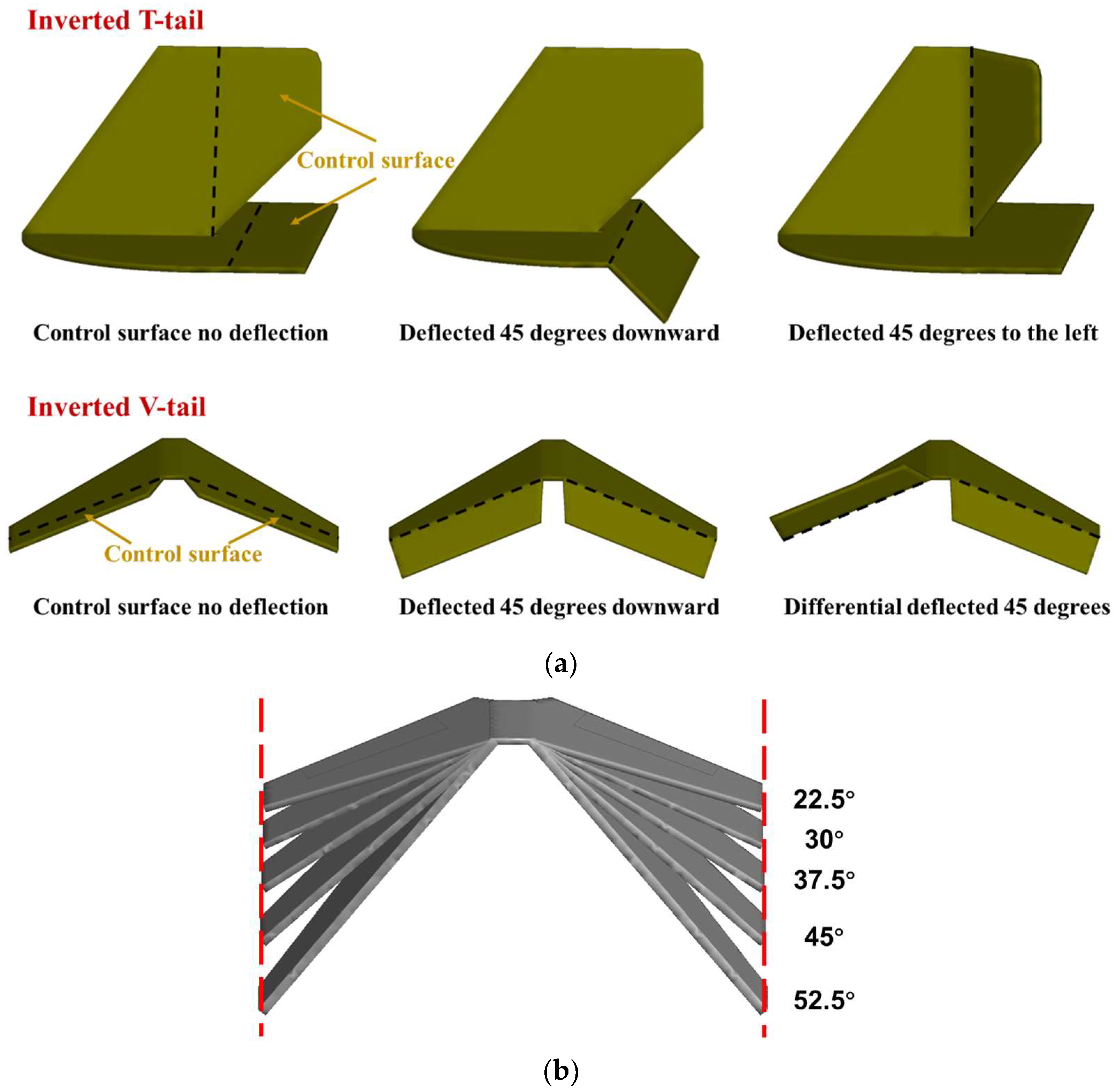
In Section 3.1.2 and Section 3.2.1, the changes of control moment caused by the deflection of the tail control surfaces are studied, and the tail models of undeflected and deflected are shown in Figure 4a. In Section 3.2, the static stability of the inverted V-tail with different dihedral angles is studied. The simulation model is shown in Figure 4b.
2.3. CFD Method
Due to the extra complexity caused by wing flexibility, most earlier works focused only on rigid wings or prescribed deformable wings. However, recently, interest in this topic has grown, and there are an increasing number of studies regarding truly flexible wings, both experiments and numerical simulations [19].
A flexible airfoil deformation law was necessary due to the weak rigidity and the limitation at the root of the wings. In a previous study [20], the rigid kinematic wing motion characteristics could not be matched with the experimental measurements, and the upper and lower wings always had a large spacing in the flapping process, which affected the simulation accuracy. The deformation of a flexible wing used in this paper draws on the research [21,22] of two-winged FMAVs. The motion of flexible wing is defined by Equations (1) and (2).
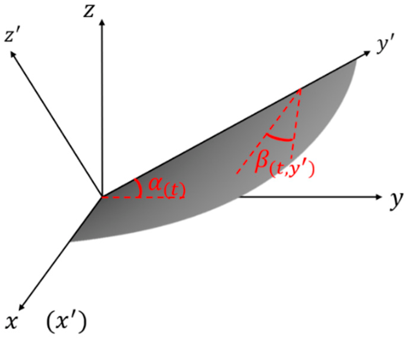
where is the flapping angle, is the flapping frequency, and is the chord torsion angle that changes linearly with the span. and are, respectively, the maximum torsion angles in the instroke and outstroke stage, which are generally obtained from experiments or fluid–structure coupling simulations. r is the spanwise position setup by the test or simulation. y’ is the distance of the section from the wing root. n is a positive integer. T is the flapping period,
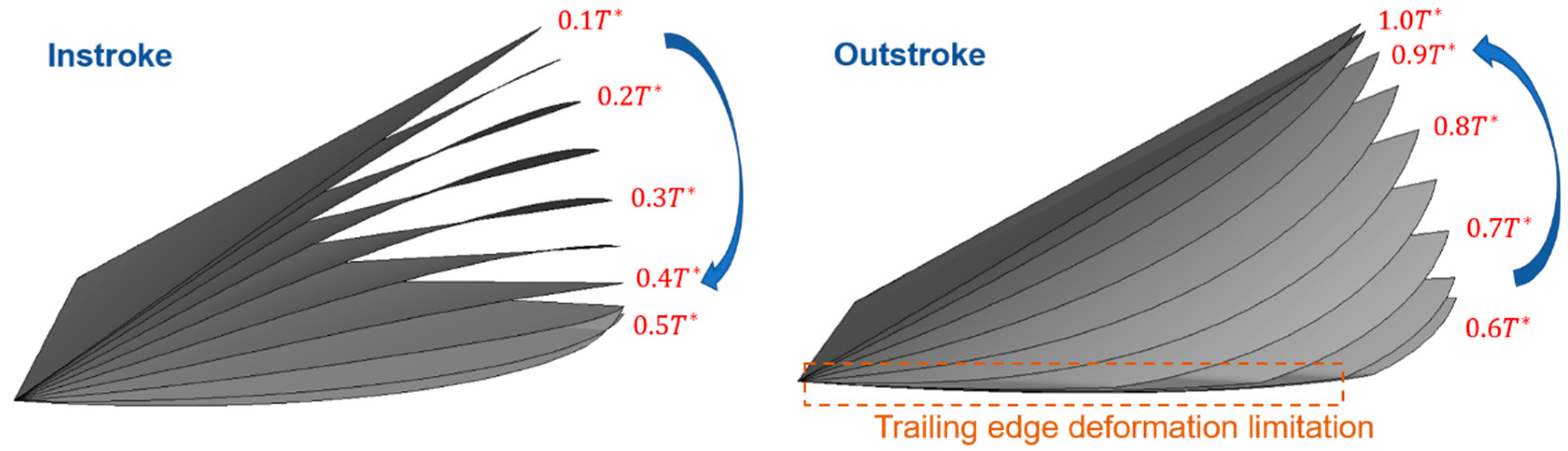
During the initial phase of the outstroke, the trailing edge deformation of the wings is limited. The coordinate system of the wings is shown in Figure 5, and the deformation of the wings during flapping is shown in Figure 6.
The Reynolds number () in this research is defined in Equation (4).
where is the fluid density, is the characteristic length, is the reference velocity, and is the dynamic viscosity of air. Similar to fixed-wing aerodynamics, the mean chord length is utilized as the reference length. is taken as the maximum value of incoming flow velocity and wing tip velocity in this study. Reynolds number in this research was between 50,000 and 100,000.
Incompressible Reynolds-averaged Navier–Strokes (RANS) equations were solved using the finite volume method. The simulation software was Fluent 2020, and the calculation method was based on the dynamic mesh method. The pressure-based method, which is faster and has better convergence in solving a low-speed incompressible flow, was used for the calculation. The turbulence model used the SST model, which was validated in previous works as suitable for calculating low Reynolds number of 3D flapping wing aerodynamics [23,24]. The total number of grids was approximately 1,500,000. The thickness of viscous boundary layer is ∼0.6 mm. The height of the first grid of the boundary layer is maintained at 0.05 mm, which meets the requirement of Y+ ∼1. The grid height ratio is 1.05 to meet the requirement of arranging enough layers of grids (layers > 10).
Using tetrahedral mesh elements combined with the dynamic mesh method provides this method with good boundary adaptability. The combination of spring smoothing and remeshing methods ensured that the quality of the nearby meshes were maintained during the movement of the flapping wing. The wings were initially at their maximum flapping amplitude for the initial simulation state.
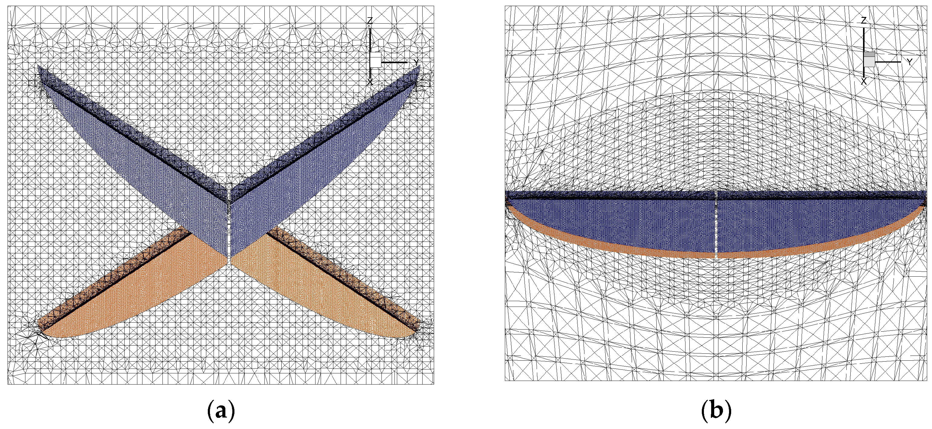
Since the flapping wing was quite thin, the airfoil shape used a flat plate without any thickness. To ensure that the simulation was as close to the real situation as possible, the minimum distance during movement was 0.002 m, where the upper and lower wings were almost touching. The calculation domain was a cuboid with a size of 30c × 20c × 20c, where c is the chord length of the flapping wing. The calculation time step was set to 0.0002 s. The computation grids for the simulation are shown in Figure 7. The simulation method was the same as the following verification method.
The following defines the dimensionless quantities in this research.
Lift coefficient,
Drag coefficient,
Moment coefficient,
Dimensionless time,
Dimensionless velocity,
where V is velocity of incoming flow, S is the surface area of wings. l is the moment reference length which is defined as the distance from the tail to the leading edge of the wings in the following section. The reference velocity in this study is 4 m/s. The reference point of the moment is set at the midpoint of the leading edge of the flapping wing (the origin of the coordinate system).
2.4. Numerical Methods Validation
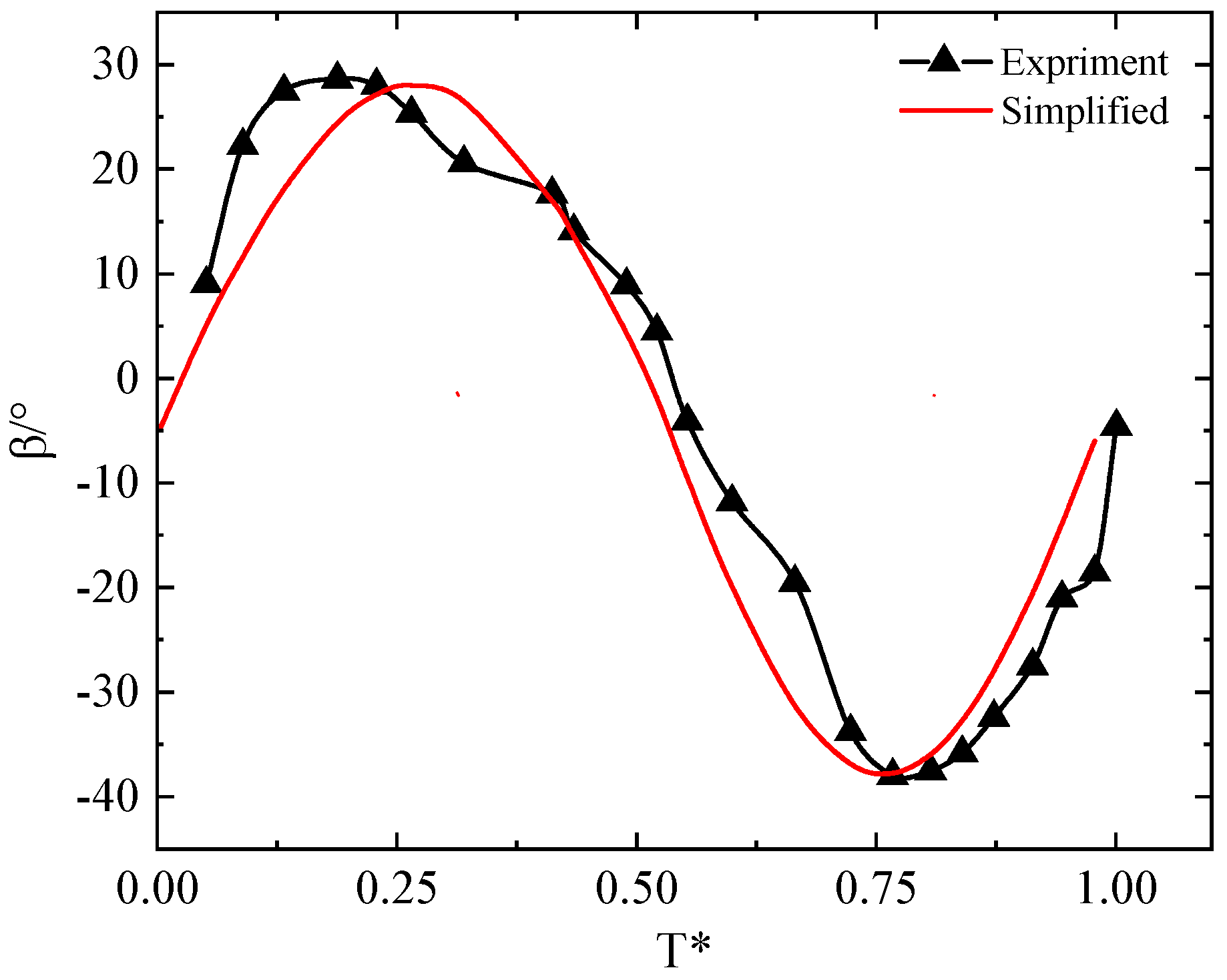
The numerical example in this study used the test results of DelFly [25] to verify the numerical method. DelFly II has a wingspan of 28 cm and a root chord length of 8.8 cm, which are similar to those of the model studied in this research. The flapping frequency in the experiment is 12 HZ, so the Reynolds number is also similar to that of this study. A high-speed camera was used to measure the deformation of the flexible wings at each stage of the flapping. The simulation conditions were consistent with the experiment. In this section of the experiment, we simplified the measured deformation of the wings to obtain the periodic aerodynamic force of the flapping wing and compared it with the experimental measurement values. We assumed that the chordwise torsion angle of the wing increases linearly outward along the span based on experimental observations. The change in the chordal torsion angle was simplified to a combination of two sine functions of different amplitudes. The simplified torsion angle and experimental values are shown in Figure 8 [25].
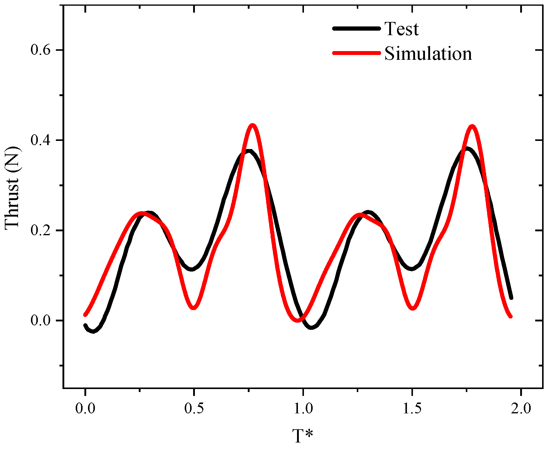
The time-varying aerodynamic thrust of the period hardly changed after calculating 6 periods. The final result is shown in Figure 9. The simulation results were consistent with the experimental results. The average periodic thrust obtained by the simulation was 0.169 N, for which the difference was within 1% when comparing with the experimental results (0.17 N). This indicates that the method adopted has high precision.
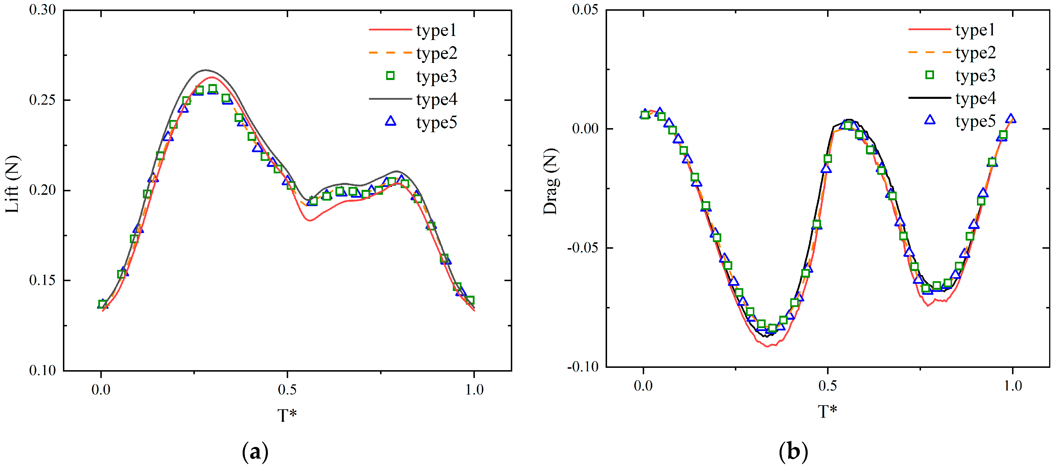
Grid and time-step convergence tests were also carried out, as shown in Figure 10. The convergence study used the simulation conditions in Section 3.1.1 (4 m/s velocity, 0° angle of attack). Three types of grids and three types of time-step sizes were tested, and their corresponding time-averaged forces were provided in Table 3. The results showed that type-2 and type-3 were highly similar for different number of grids, and the results of type-2 and type-5 with different time-step sizes were also highly similar. Thus, for efficient computation, the type-2 grid and type-2 time-step size were selected for the subsequent simulations.
3. Results and Discussions
In this section, the aerodynamic characteristics of the wings and tails are discussed. The contribution of the tail to the stability and maneuvering of the aircraft is analyzed. Then, the relationship between the tail layout and maneuvering characteristics is studied by changing the tail-installation position. Finally, the aerodynamic interaction mechanism of the wings and tail is explained in detail, according to the results of the flow field analysis.
Table 4 is a general overview of the simulation conditions in each section.
3.1. Analysis of Aerodynamic Characteristics
3.1.1. Force Characteristics
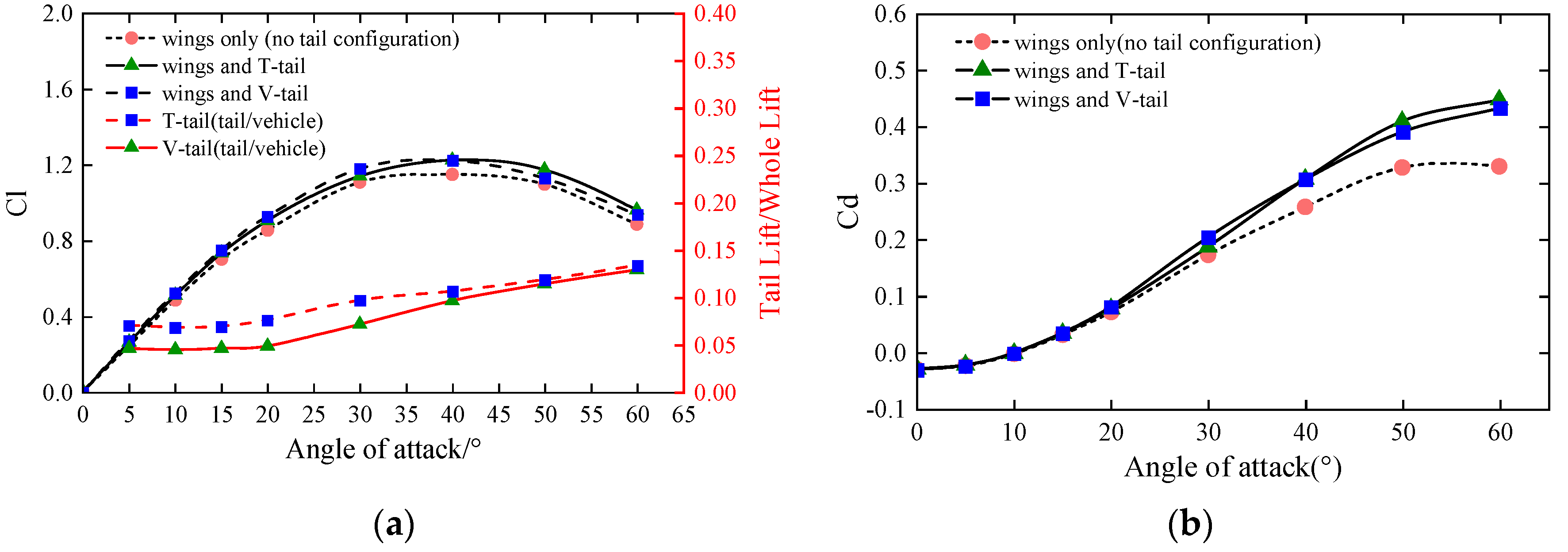
First, the aerodynamic characteristics of the flapping wing were analyzed by applying changes to angle of attack (0° to 60°). The force characteristics of the flapping wing with the two types of tails were calculated in a fixed incoming flow velocity (4 m/s). Figure 11 shows the aerodynamic force of the whole vehicle at different angles of attack. The two types of tails had no obvious influence on the lift coefficient slope, maximum lift coefficient, or zero-lift drag coefficient of the whole aircraft. When the angle of attack was less than 20°, the ratio of the tail lift to the whole lift of the vehicle changed within a small range, by approximately 4.6% for the inverted T-tail and by approximately 7.1% for the inverted V-tail. As the flapping wings were located in front of the tail, the wings were less affected by the tail. The curve of the flapping wing’s lift versus the angle of attack was similar to a straight line, and the slope of the lift line was approximately 2.47. As the angle of attack gradually increased, when the angle of attack was greater than 20°, the proportion of the tail lift increased approximately linearly, and the tail drag increased rapidly.
Compared with the fixed-wing configuration at the same Reynolds number, the flapping-wing vehicle had a better stall performance owing to the delayed stall mechanism. From the lift and thrust curves, it can be seen that when the flapping wing was cruising in flight at a velocity of 4 m/s and at a 10° angle of attack, the lift and thrust generated by the flapping wing were in balance with gravity and drag, respectively.
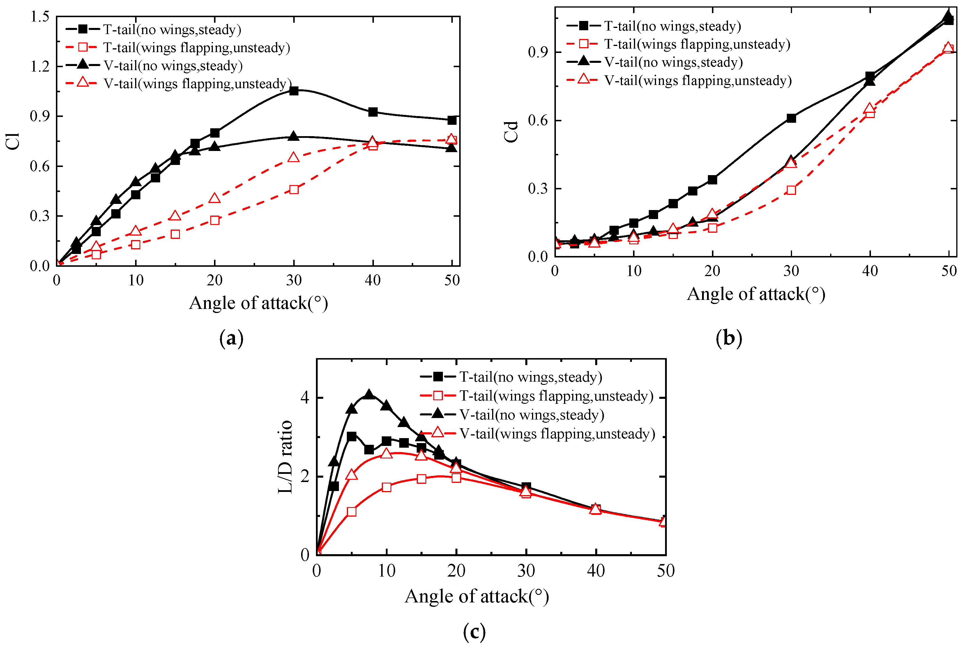
The lift and drag of the tails in steady and unsteady conditions was compared, as shown in Figure 12. The steady setting was that the tail was only affected by the uniform incoming flow. It can be clearly seen that the tails were disturbed by the unsteady incoming flow, and the lift–drag characteristics showed clear changes. For the inverted T-tail, the aerodynamic efficiency was greatly reduced; the tail lift-line slope was reduced from 2.49 to 0.75, and the maximum L/D ratio was reduced from 3.02 to 1.96. The angle of attack that corresponds to the maximum L/D ratio shifted backward. The inverted V-tail aerodynamic characteristics were also significantly degraded. Therefore, it is necessary to consider the flapping interference in the aerodynamic modeling of tails.
The drags of two tails were similar in Figure 12b. However, the maximum L/D ratio of the inverted V-tail was 47.4% greater than that of the inverted T-tail. In Section 3.3, the reasons for the different changes in the aerodynamic characteristics of the two tails are discussed based on the results of the flow field analysis.
3.1.2. Moment Characteristics
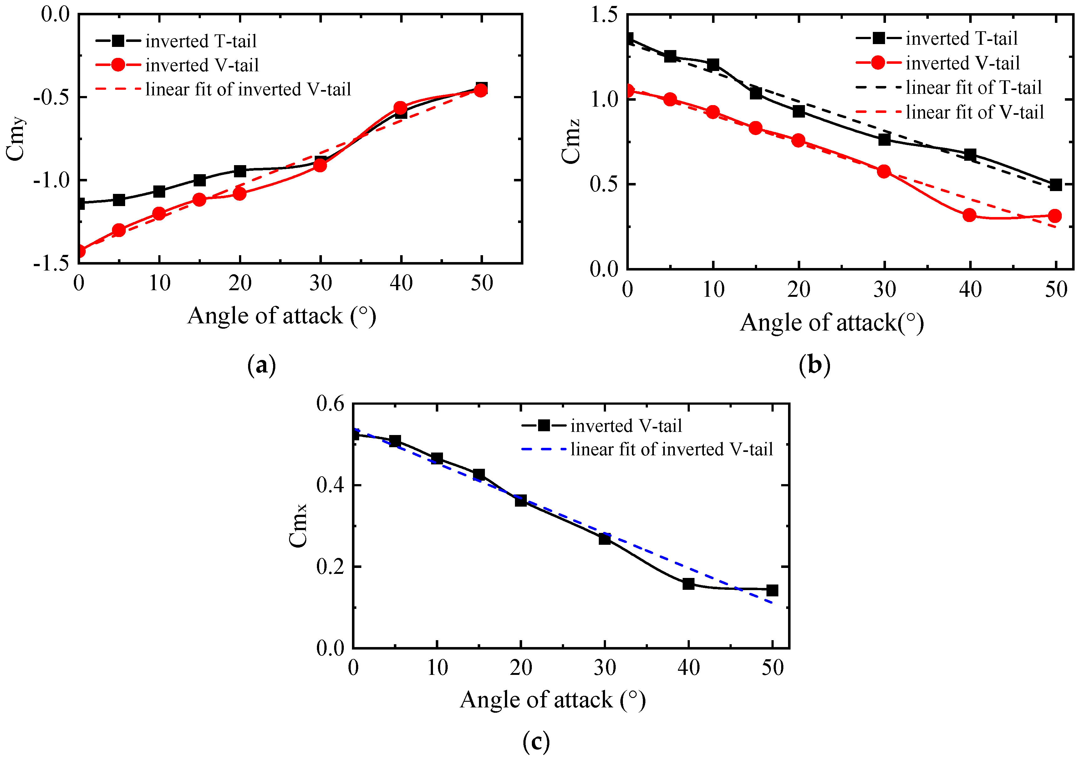
In the forward flight state at 4 m/s velocity, the control moment of the tails decreased continuously with the increase in the angle of attack. Figure 13 shows the curve of the control moment changing with the angle of attack when the inverted T-tail and V-tail deflected 45°. The three moments were approximately linear and decreased rapidly, that is, the control effects caused by the tail control surfaces at a large angle of attack were weak.
When the angle of attack was less than , the pitch moment of the inverted T-tail decreased relatively slowly due to the effect of the wake reducing the incoming angle. When the angle of attack was greater than , the pitch moments of the two tails were almost the same. Due to the lateral-directional coupling of the inverted V-tail, the yaw moment was slightly smaller than the inverted T-tail, but, at the same time, it produced a roll that was beneficial to the aircraft’s lateral-directional maneuvering and improved flight performance. In a cruising state (4 m/s, 10°), the pitch control moment of inverted V-tail is 12.8% greater than that of the inverted T-tail. Although the directional control moment is 23% lower, it generates a positive roll moment of 50% of the value of the directional moment at the same time, which is beneficial for maneuvering.
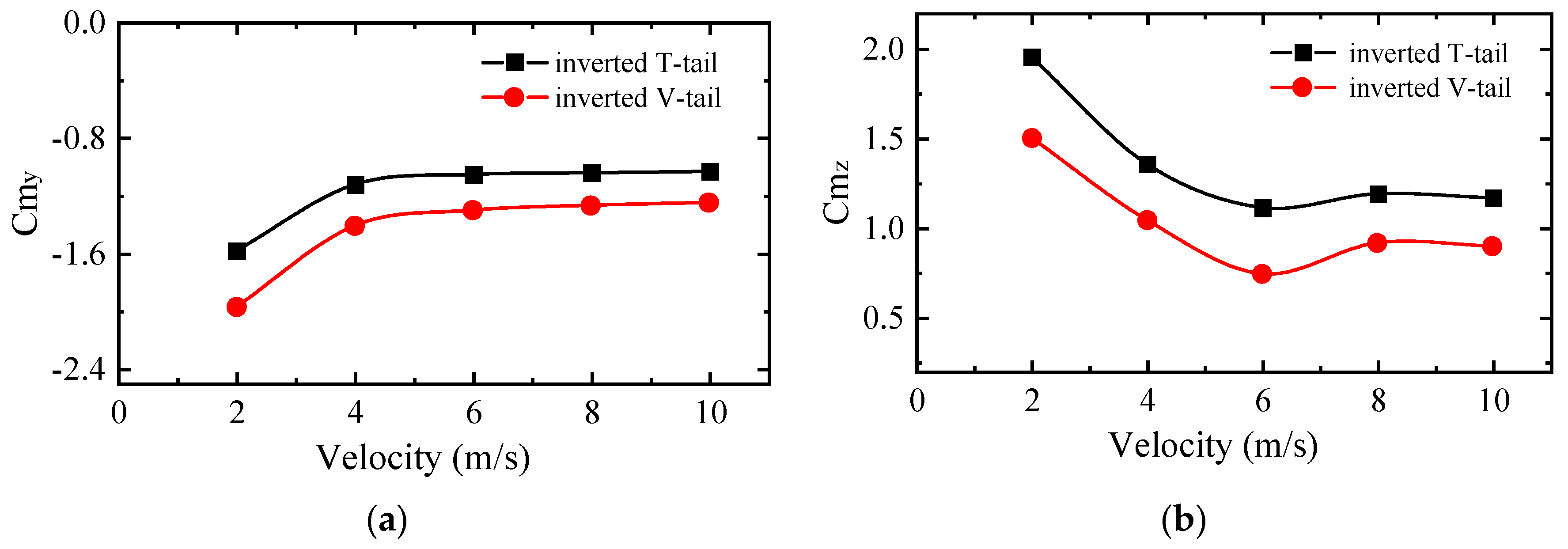
In this section, the control moment characteristics under different inlet velocities are also discussed. The inlet velocity range was set as 0 m/s to 10 m/s, and the angle of attack was 0. The pitching moment coefficient decreased with increasing incoming flow velocity, as shown in Figure 14. When the incoming flow velocity was less than 4 m/s, the tail was significantly affected by flapping, and the pitching moment coefficient was larger than the coefficient at a faster speed. At this time, the pitching moment coefficient decreased rapidly with an increasing velocity. As the velocity increased to more than 6 m/s, the wing flapping had a smaller effect on the tail control, and the moment coefficient changed little with the incoming velocity. Under all the speed conditions, the pitching moment of the inverted V-tail was always better than that of the inverted T-tail. The trend of the yaw moment was similar to that of the pitch moment.
3.1.3. Analysis of Longitudinal Static Stability
The position of the aerodynamic center is very important for the longitudinal stability of the aircraft. By calculating the aerodynamic characteristics of the X-shaped flapping wing in different flight conditions, the pressure center and aerodynamic center of the aircraft can be obtained. Since flapping-wing vehicles often fly at low Reynolds numbers and high angles of attack [26], the influence of drag/thrust needs to be considered when calculating the aerodynamic center. When calculating the static stability of the vehicle, the control surfaces of two types of tails do not deflect.
Considering the thrust, the pressure center position and the aerodynamic center position, respectively, are
where M is the pitching moment, L is the lift force, D is the drag force, θ is the angle of attack. , and is the change of the angle of attack. All of these can be obtained by a prior simulation.
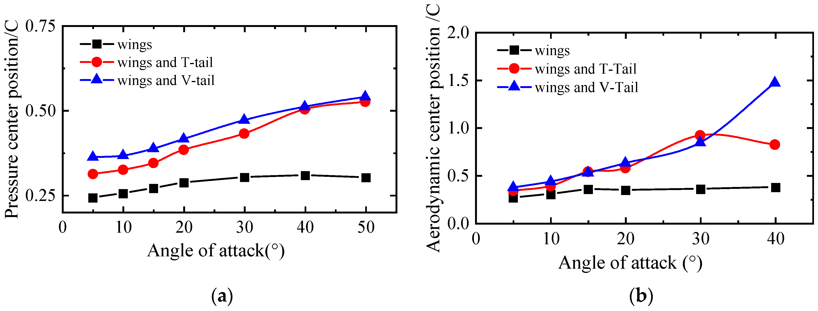
The positions of the pressure and aerodynamic centers are shown in Figure 15a,b, respectively. The pressure center of the wings was initially located at 0.25C (0.25 times the chord length of the wings) and increased slowly with the increasing angle of attack. When the angle of attack was greater than 30°, the pressure center of the wings hardly changed and was finally located near the position of 0.3C. The aerodynamic center changed relatively little and was always approximately 0.3C.
For flapping-wing vehicles with a tail, the pressure and aerodynamic center changed significantly with the increasing angle of attack, and the pressure center continued to move backward.
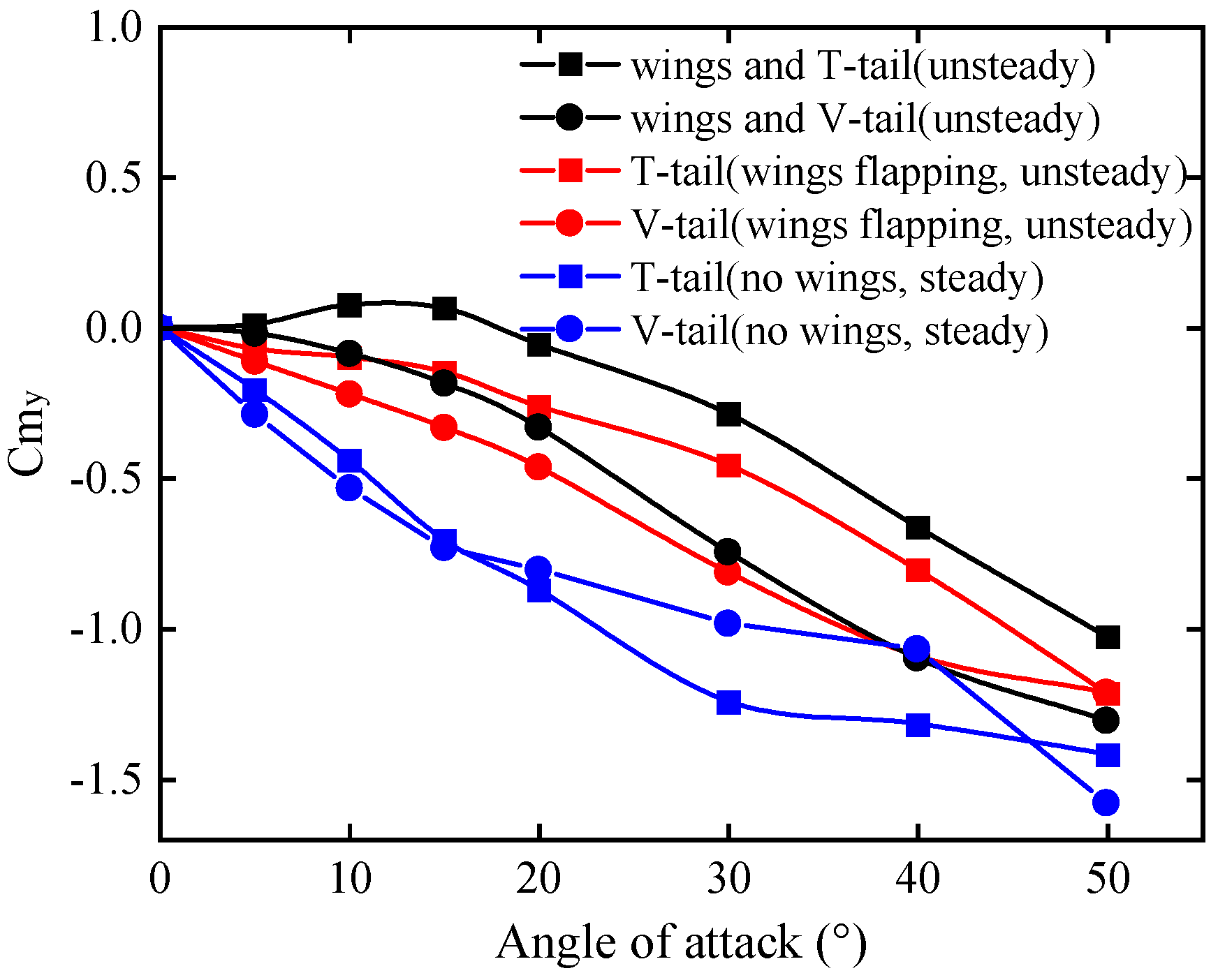
The gravity center of the vehicle was located 3.15 cm from the leading edge, which was used to analyze the longitudinal static stability of the vehicle. Figure 16 shows the longitudinal static stability of vehicles with different tails. Although the presence of tails can greatly increase the longitudinal static stability, the unsteady incoming flow under the interference of the wings greatly reduced the longitudinal stable effect of the tail. Compared with the steady state, the longitudinal restoring moment of the inverted T–tail was reduced by approximately 75% within the range of the 0° to 15° angle of attack, and the inverted V-tail was reduced by approximately 60%.
The slope of the longitudinal moment curve with an inverted V-tail was obviously greater than that with an inverted T-tail when the angle of attack was less than 30°. This indicates that the vehicle with an inverted V-tail had better longitudinal static stability and a greater stable moment. This is mainly because the inverted T-tail was greatly affected by the wake, which reduced the incoming local angle in front of the tail. With angle of attack in the range of 0° to 15°, the vehicle with an inverted T-tail exhibited longitudinal static instability, so the center of gravity would need to be moved forward in actual flight.
3.1.4. Analysis of Lateral Static Stability
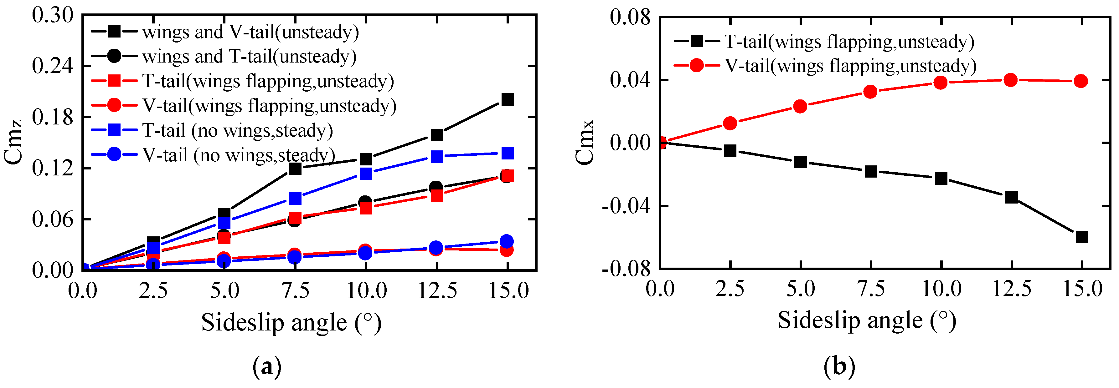
This section compares the lateral stability of the two tails with the same projection area. The incoming velocity was set to 4 m/s at a 10° angle of attack, and the angle between the flow and body axis changed from 0° to 20°.
The directional stable moment changed approximately linearly with the body side-slip angle, as shown in Figure 17a. An unsteady incoming flow had little effect on the directional moment by the inverted V-tail. However, this reduced the directional restoring moment of the inverted T-tail by approximately 25%. The directional restoring moment of the inverted V-tail was only one-third that of the inverted T-tail. The directional stability of the vehicle with an inverted V-tail was only 55% of that of the vehicle with an inverted T-tail. Therefore, to achieve the same stability, it is necessary to increase the vertical projection area of the V-tail. However, the wetted area of the tail will also increase at this time.
Figure 17b shows the analysis of the lateral static stability of the vehicle. It can be seen from the figure that the inverted V-tail had a positive effect on the lateral stability of the aircraft, while the inverted T-tail had the opposite effect. Due to the asymmetry of the incoming flow, both the horizontal tail and the vertical tail of the inverted T-tail will produce opposite rolling moments, resulting in lateral static instability. At this time, it is necessary to adjust the control surface to increase the lateral stability of the aircraft.
3.2. Influence of the Tail Layouts on the Aerodynamic Characteristics
3.2.1. Effect of Tail Position on the Control Moment
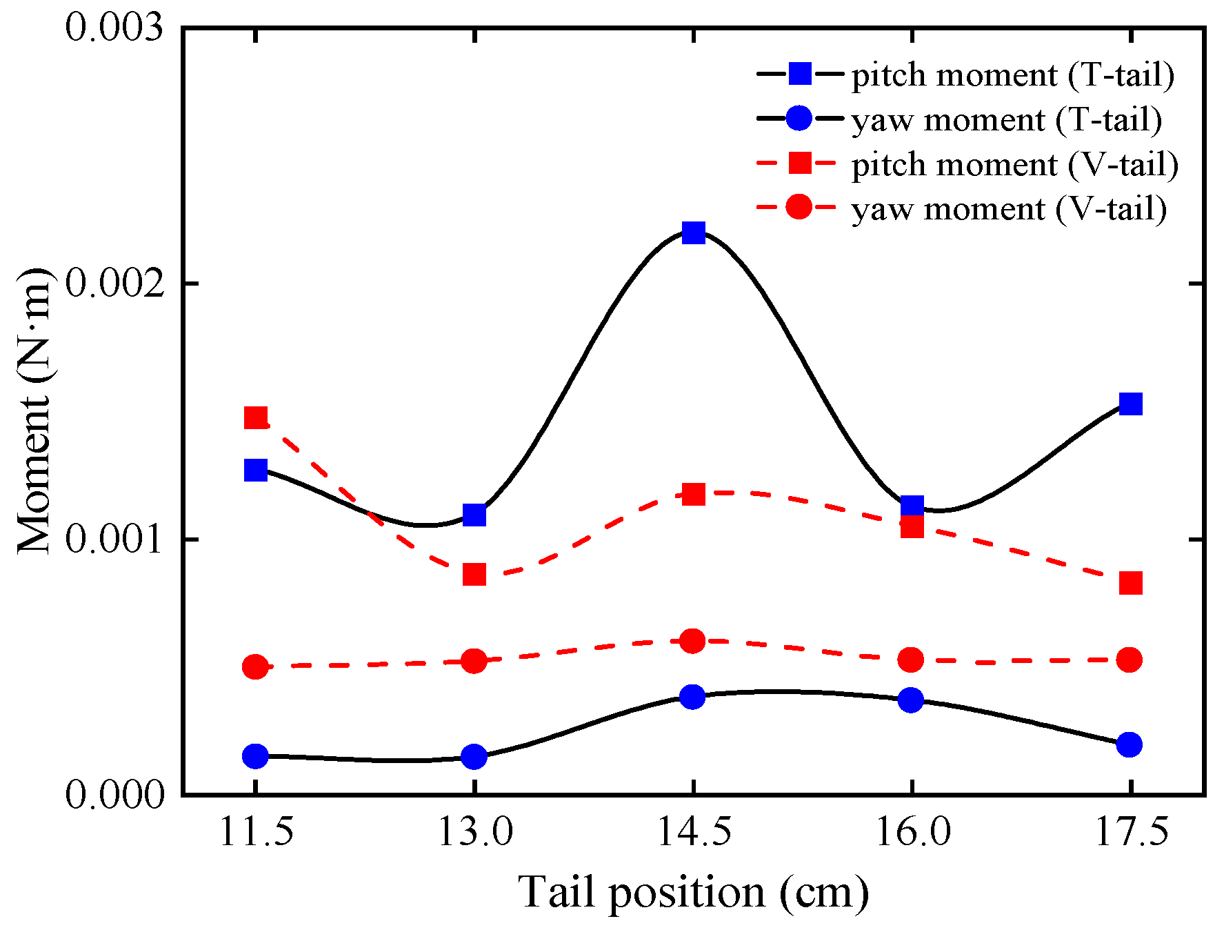
The control efficiency of the tail depends on the forward flow relative to the tail. In general, the greater the flow speed is, the stronger the control ability of the tail. However, at a forward speed of 0 m/s, for instance, the flapping wing was hovering, and the tail still needed to have sufficient maneuverability. Therefore, the simulation condition in this section was set to 0 m/s. By changing the positions of the tails, the aerodynamic characteristics were obtained. In the simulation, the distance between the leading edge and tails was set from 11.5 cm to 17.5 cm in intervals of 1.5 cm.
The tail used the accelerating gas generated by the flapping wings to generate the control moment. When the tail was close to the flapping wing, the aerodynamic influence of the flapping wing is greater; additionally, the aerodynamic force arm of the tail was also smaller.
The pitching and yaw moment results are shown in Figure 18. When the leading edge of the tail was 14.5 cm away from the leading edge of the flapping wing, the pitching and yaw moments of the inverted T-tail were the absolute maximum, the yaw moment of the inverted V-tail was the absolute maximum, and the pitching moment was locally maximized. At the optimal position, the moment of the inverted T-tail was nearly doubled as compared with the initial position. The horizontal tail volume coefficient and vertical tail volume coefficient were 0.31 and 0.027, respectively, at this time.
The maximum pitching moment of the inverted T-tail is nearly twice that of the inverted V-tail. The maximum yaw moment of the inverted V-tail is 50% stronger than that of the inverted T-tail. Due to the symmetry of the flapping wing vehicle, the longitudinal moment control capability is of greater concern. Therefore, the inverted T-tail is more suitable to be selected at low speed and hovering conditions.
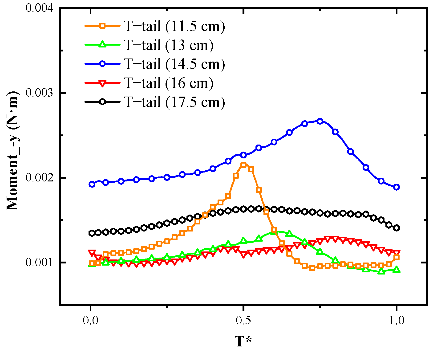
The farther the tail position, the smaller the degree of undulation of the control moment was, so the unsteady effect became weaker. The pitch moment time-history of the inverted T-tail in different tail positions is shown in Figure 19. When the tail position was located at 17.5 cm, the mean value of the moment was larger, and the fluctuation of the moment was relative minimum. When the tail position was located at 11.5 cm, it was strongly disturbed by the flapping wing, and the variation of the moment within the period was the largest. As the tails moved away from the flapping wing, the phase of the peak moment also shifted back.
3.2.2. Effect of V-Tail Dihedral Angle on Directional Static Stability
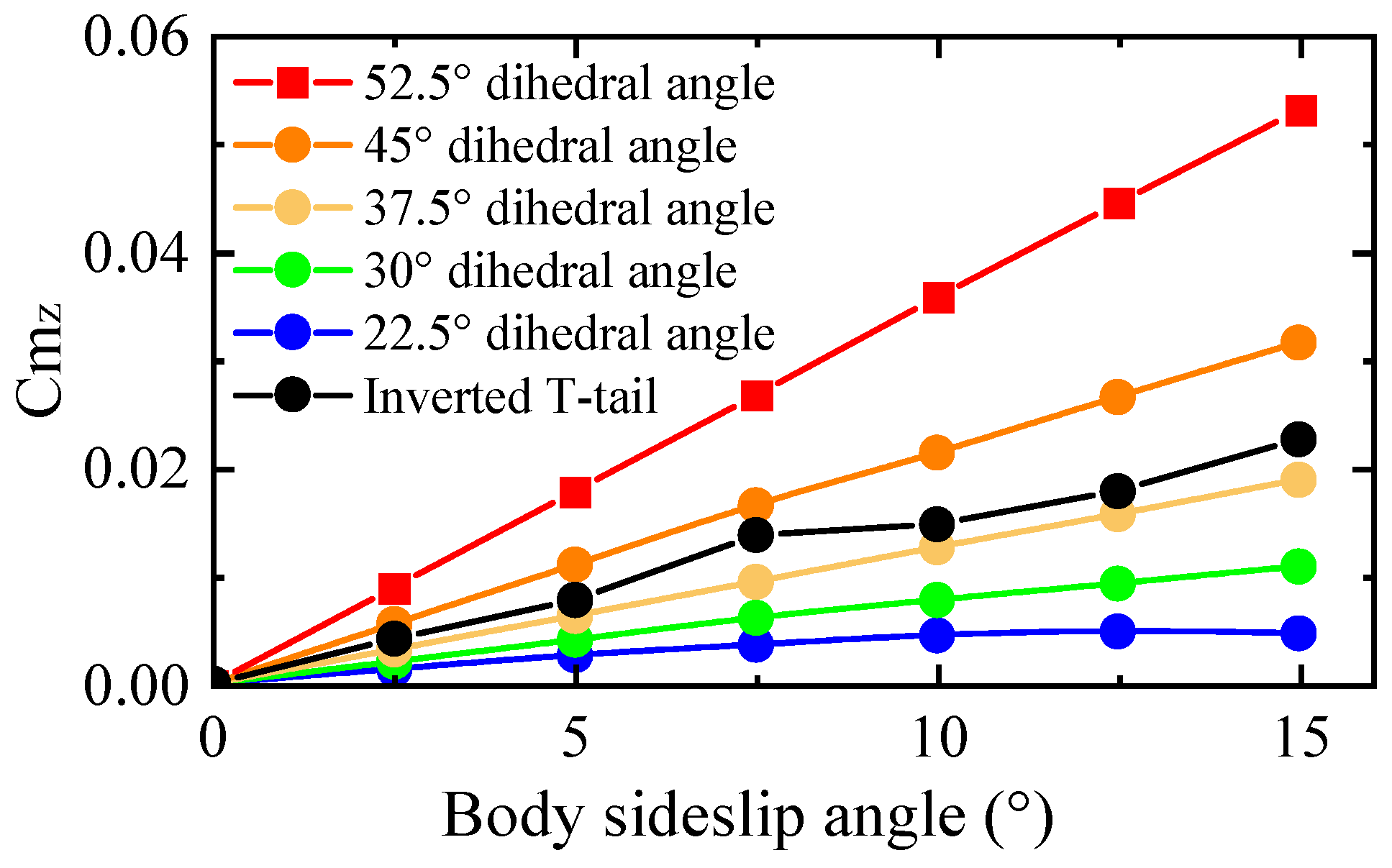
The vertical stabilizer area can affect the directional stability of the aircraft. For the inverted V-tail, the larger the dihedral angle λ is, the stronger the directional static stability. The following compares the directional stability of the inverted V-tail with five dihedral angles.
The directional stability was relatively less disturbed by the flapping wing wake, so the restoring moment changed with the side-slip angle, showing good linear characteristics, as shown in Figure 20. Increasing the dihedral angle of the V-tail effectively increased the lateral force and yaw moment of the tail and improved the heading stability. As the dihedral angle increased, the heading stability gradually increased. The greater the dihedral angle is, the greater the distance of the tail surface from the most affected line, which increases the effect of the tail at the same time.
The static stability of the inverted V-tail with a 41.5° dihedral angle was similar to that of the inverted T-shaped tail. Its vertical projection area was 61.8 cm2, which was approximately 2.14 times that of the inverted T-tail.
3.3. Analysis of Flow Mechanism
The flow field under the effect of interaction between the flapping wings and tails is presented in this section, and the flow mechanism of the unsteady effects is illustrated. The reasons for the different aerodynamic characteristics of the two types of tails are also explained.
3.3.1. Clap–Peel Mechanism
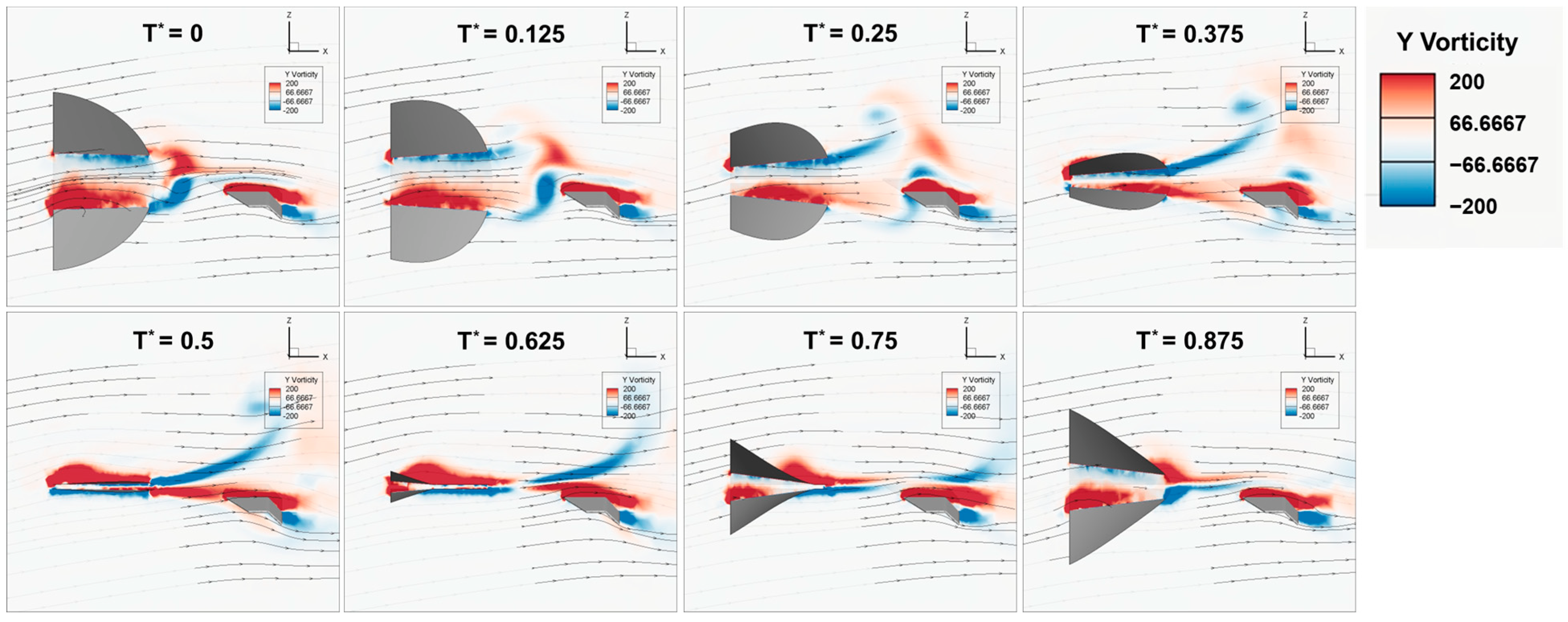
The clap–peel mechanism increases the induced flow velocity produced by the flapping wings, which periodically increases the control effect of the tail. Figure 21 represents the vorticity change and streamline change across a flapping cycle in a cruise state (4 m/s 10°). A backward momentum jet was produced due to the wings flapping, which hit the tail and increased the moment for control, making tail control more efficient.
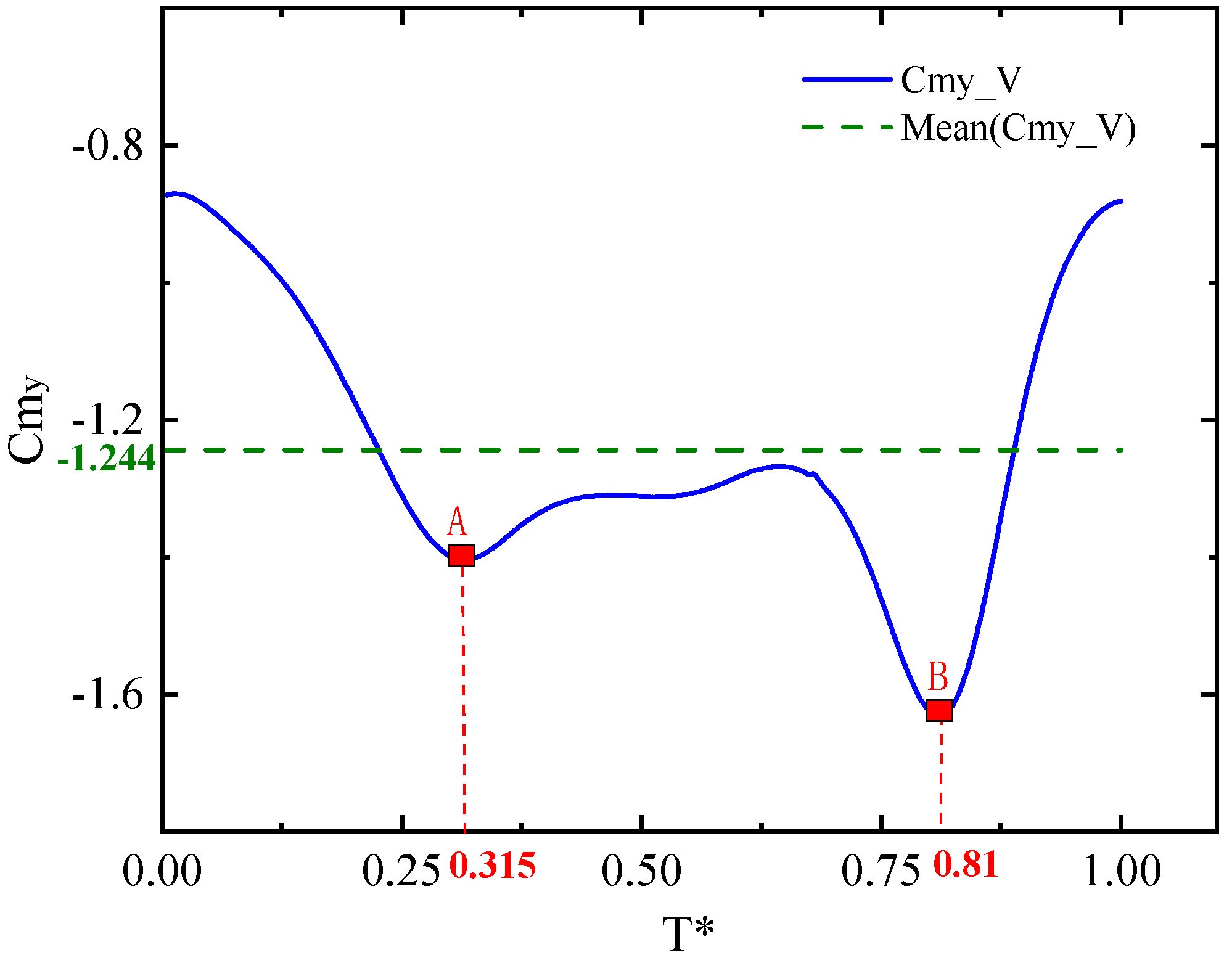
When was close to 0, the flapping wing was in a transition phase from outstrokes to instrokes. At this time, the attached vortex on the flapping wing was thrown out. The attached vortices on the outside surfaces of the wings (the upper surface of the upper flapping wing and the lower surface of the lower flapping wing) appeared to fall off and flow to the tail, resulting in an increase in the force on the tail. When was between 0.25 and 0.375, the shedding vortices moved to the vicinity of the tail. The attachment vortex on the lower surface of the tail was greatly strengthened, and the attachment vortex on the upper surface was slightly reduced, making the force on the tail appear to be at a maximum, as shown in point A in Figure 22. Then, as the vortex disappeared, the force gradually decreased.
When was approximately 0.5, the flapping wings switched from instrokes to outstrokes. The attached vortex on the flapping wing was ‘squeezed out’. The vortices of the inside surfaces of the flapping wings gradually fell off and flew to the tail. The attached vortex on the upper surface of the tail was remarkably enhanced, causing another larger peak in the force of the empennage, as shown in point B in Figure 23. Therefore, there were two maximum effects in a period. The range of the curve during a period was approximately 62% times the average pitching moment.
3.3.2. Wake Deflection Mechanism
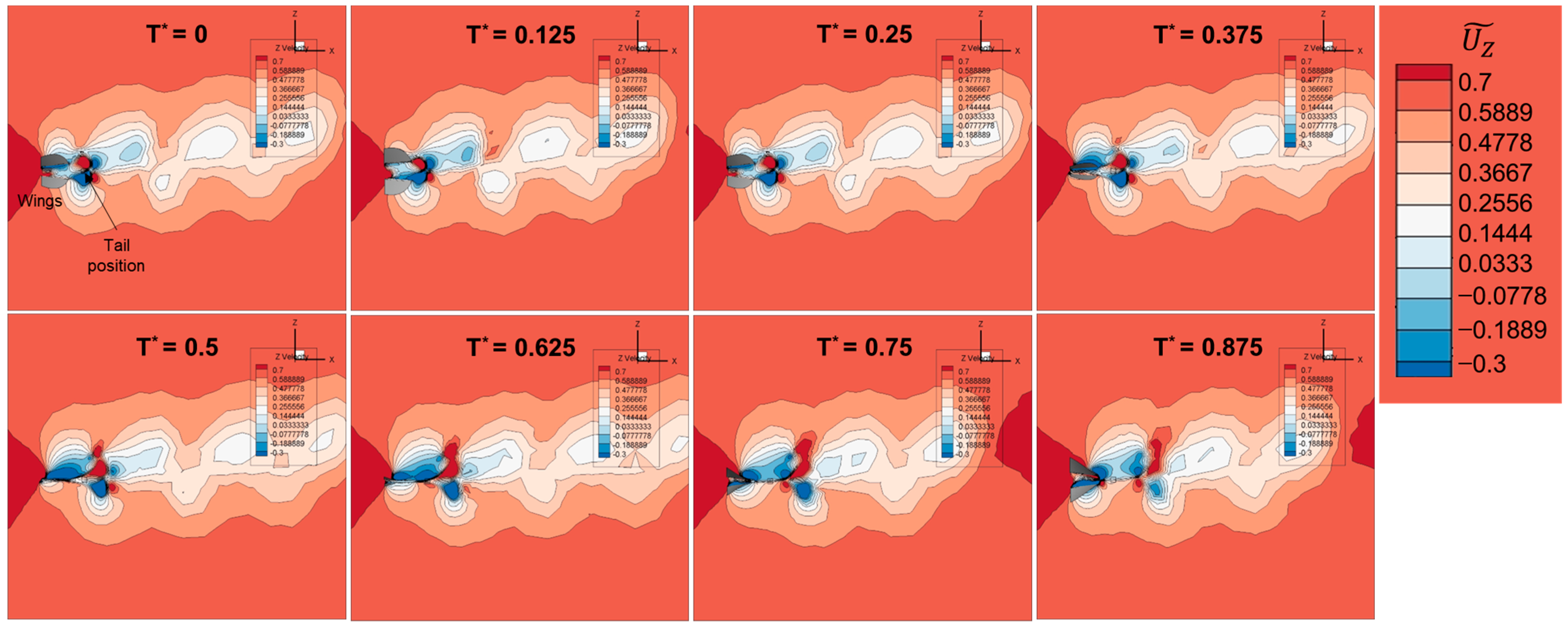
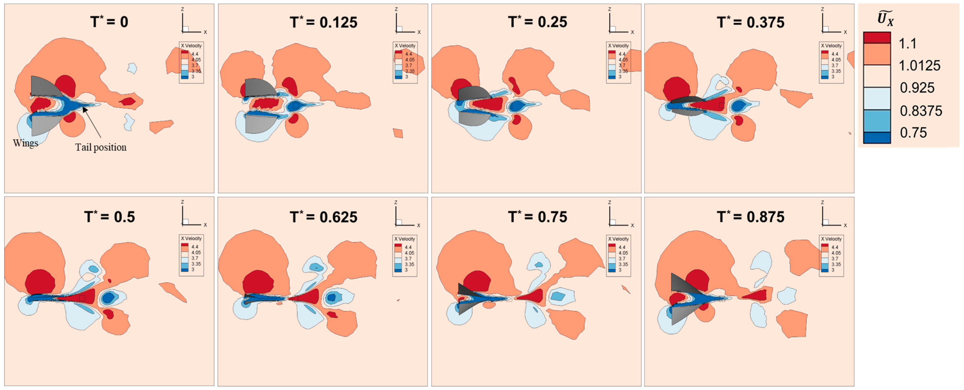
The airflow passing by the flapping wings had more downward momentum, as shown in Figure 24; in other words, the direction of the incoming flow was deflected downward and was affected by wing flapping. The direction of the interference zone was consistent with the direction of the incoming flow, and the influence degree gradually decreased from the center of the interference zone to the outside. These characteristics are the same as those for the wake of rotors in forward flight. The difference is that the influence of the wake was significantly larger than that of the rotor. When the distance from the vehicle axis was less than 1.5 times the span, the Z velocity disturbance was still greater than 15% of the maximum disturbed speed. The tail position was affected by the clap and peel of the flapping wings, where the X velocity periodically increased and decreased, as shown in Figure 25.
A considerable area behind the flapping wings was obviously disturbed by the wake, resulting in a significant reduction in the Z-direction velocity. The angle of attack of the incoming flow at the tail was close to zero. On the one hand, the reduction in the angle of attack also reduced the lift and drag of the tail. On the other hand, the decrease in angle of attack increased the stall angle of the tail, so that the tail was able to maintain a higher level of control effect when the angle is 20° or less. When the angle of attack was above 20°, the tails were farther from the line of greatest interference, so the wake interference was relatively reduced. At this time, the drag of the tail increased rapidly, which reduced the flight performance of the aircraft.
The control effect of the tails depends on the incoming flow to the tails. In the case of hovering or low-velocity flight, the incoming flow is mainly determined by the induced flow of the flapping wings. In this case, the control effect of the inverted T-tail, which was greatly affected by the wake, was stronger than that of the inverted V-tail. In contrast, when flying forward at a higher speed, the incoming flow was superimposed by the flow from afar and the induced flow. In this state, the average of the induced flow in a period was small, and its unsteady momentum jet was more likely to separate the attached vortex of tails, which reduced the L/D ratio of the tail. Affected by this, in the forward-flight state, the lift and longitudinal moment of the tail were smaller than those without wing interference. The closer the tail is to the center of the interference zone, the more dramatic the effect will be. Therefore, the longitudinal aerodynamic performance of the inverted V-tail was better than that of the inverted T-tail when flying forward at a higher speed.
4. Conclusions
In this article, the aerodynamic characteristics of an X-wing flapping vehicle of various tails of an X-wing flapping vehicle have been discussed. Based on the results of the numerical analysis, the main conclusions of this study are as follows:
- (1)
- Tails of different configurations are suitable for different flight states. In a hovering state, the maximum pitch control moment of the inverted T-tail is nearly twice that of the inverted V-tail. In a cruising state, the L/D ratio of the inverted V-tail is 47.4% higher than inverted T–tail, and the pitch control moment is 12.8% higher. The inverted V-tail produces a directional control moment with a positive lateral moment, which is beneficial to maneuvering.
- (2)
- The correct tail layout can improve flight performance. The control moments of the inverted T-tail and inverted V-tail reached the maximum when the vertical and horizontal tail volume coefficient are, respectively, 0.31 and 0.027. The directional static stability of the inverted V-tail with a 2.14-times vertical projection area is similar to that of the inverted T-tail.
- (3)
- In this paper, a simplified flexible deformation is proposed for X-shaped flapping wings, and the simulation results are in good agreement with the experimental results.
This study provides support for the tail design of X-shaped flapping wings.
Author Contributions
Conceptualization, H.L. and D.L.; methodology, H.L. and Z.K.; software, H.L. and D.B.; validation, Z.K.; formal analysis, H.L.; investigation, T.S.; resources, H.L. and T.S.; data curation, H.L.; writing—original draft preparation, H.L.; writing—review and editing, Z.K. and D.B.; visualization, H.L.; supervision, T.S.; funding acquisition, D.L. All authors have read and agreed to the published version of the manuscript.
Funding
This research was funded by the National Natural Science Foundation of China, grant number 11972059.
Institutional Review Board Statement
Not applicable.
Informed Consent Statement
Not applicable.
Data Availability Statement
Not applicable.
Conflicts of Interest
The authors declare no conflict of interest.
Abbreviations
The following abbreviations are used in this manuscript:
| L/D ratio | Lift to drag ratio |
| FMAV | Flapping wing micro aerial vehicle |
| CFD | Computational fluid dynamic |
| RANS | Reynolds-averaged Navier–Strokes |
| C.G | Center of gravity |
References
- Guo, S.; Li, D.; Wu, J. Theoretical and Experimental Study of a Piezoelectric Flapping Wing Rotor for Micro Aerial Vehicle. Aerosp. Sci. Technol. 2012, 23, 429–438. [Google Scholar] [CrossRef]
- Li, D.; Guo, S.; Di Matteo, N.; Yang, D. Design, Experiment and Aerodynamic Calculation of a Flapping Wing Rotor Micro Aerial Vehicle. In Proceedings of the 52nd AIAA/ASME/ASCE/AHS/ASC Structures, Structural Dynamics and Materials Conference, Denver, CO, USA, 4–7 April 2011; pp. 1–10. [Google Scholar] [CrossRef]
- Karasek, M.; Muijres, F.T.; De Wagter, C.; Remes, B.D.W.; De Croon, G.C.H.E. A Tailless Aerial Robotic Flapper Reveals That Flies Use Torque Coupling in Rapid Banked Turns. Science 2018, 361, 1089–1094. [Google Scholar] [CrossRef] [PubMed]
- Deng, S.; Wang, J.; Liu, H. Experimental Study of a Bio-Inspired Flapping Wing MAV by Means of Force and PIV Measurements. Aerosp. Sci. Technol. 2019, 94, 105382. [Google Scholar] [CrossRef]
- Jones, K.D.; Bradshaw, C.J.; Papadopoulos, J.; Platzer, M.F. Improved Performance and Control of Flapping-Wing Propelled Micro Air Vehicles. In Proceedings of the 42nd AIAA Aerospace Sciences Meeting and Exhibit, Reno, NE, USA, 5–8 January 2004; pp. 360–370. [Google Scholar] [CrossRef]
- Tay, W.B.; Van Oudheusden, B.W.; Bijl, H. Numerical Simulation of X-Wing Type Biplane Flapping Wings in 3D Using the Immersed Boundary Method. Bioinspiration Biomim. 2014, 9, 17–19. [Google Scholar] [CrossRef] [PubMed]
- Ma, K.Y.; Chirarattananon, P.; Fuller, S.B.; Wood, R.J. Controlled Flight of a Biologically Inspired, Insect-Scale Robot. Science 2013, 340, 603–607. [Google Scholar] [CrossRef] [PubMed]
- Ramezani, A.; Chung, S.J.; Hutchinson, S. A Biomimetic Robotic Platform to Study Flight Specializations of Bats. Sci. Robot. 2017, 2, eaal2505. [Google Scholar] [CrossRef] [PubMed]
- Keennon, M.; Klingebiel, K.; Won, H.; Andriukov, A. Development of the Nano Hummingbird: A Tailless Flapping Wing Micro Air Vehicle. In Proceedings of the 50th AIAA Aerospace Sciences Meeting including the New Horizons Forum and Aerospace Exposition, Nashville, TN, USA, 9–12 January 2012. [Google Scholar] [CrossRef]
- Doman, D.B.; Oppenheimer, M.W.; Sigthorsson, D.O. Wingbeat Shape Modulation for Flapping-Wing Micro-Air-Vehicle Control during Hover. J. Guid. Control Dyn. 2010, 33, 724–739. [Google Scholar] [CrossRef]
- Jiao, Z.; Wang, L.; Zhao, L.; Jiang, W. Hover Flight Control of X-Shaped Flapping Wing Aircraft Considering Wing–Tail Interactions. Aerosp. Sci. Technol. 2021, 116, 106870. [Google Scholar] [CrossRef]
- Grauer, J.A. Modeling and System Identification of an Ornithopter Flight Dynamics Model; University of Maryland: College Park, MD, USA, 2012. [Google Scholar]
- Tay, W.B.; Bijl, H.; Van Oudheusden, B.W. Biplane and Tail Effects in Flapping Flight. AIAA J. 2013, 51, 2133–2146. [Google Scholar] [CrossRef]
- Yangang, W.; Weixiong, C.; Shuanghou, D.; Xuming, Z. Numerical Study of Flapping Wing/Tail Aerodynamic Interaction for Flapping Wing Micro Air Vehicle. J. Aerosp. Power 2015, 30, 257–264. [Google Scholar]
- Deng, S.; Van Oudheusden, B. Wake Structure Visualization of a Flapping-Wing Micro-Air-Vehicle in Forward Flight. Aerosp. Sci. Technol. 2016, 50, 204–211. [Google Scholar] [CrossRef]
- Yin, Y.; Dong, L.; Zhenhui, Z. Influences of Flapping Wing Micro Aerial Vehicle Unsteady Motion on Horizontal Tail. Acta Aeronaut. Astronaut. Sin. 2012, 33, 1827–1833. [Google Scholar]
- Percin, M.; Eisma, H.E.; Van Oudheusden, B.W.; Remes, B.; Ruijsink, R.; de Wagter, C. Flow Visualization in the Wake of Flapping-Wing MAV “Delfly II” in Forward Flight. In Proceedings of the 30th AIAA Applied Aerodynamics Conference, New Orleans, LA, USA, 25–28 June 2012; pp. 132–143. [Google Scholar] [CrossRef]
- Decroon, G.C.H.E.; Perçin, M. The Delfly: Design, Aerodynamics, and Artificial Intelligence of a Flapping Wing Robot; Springer: Berlin/Heidelberg, Germany, 2015; pp. 15–16. [Google Scholar] [CrossRef]
- Xu, M.; Wei, M.; Yang, T.; Lee, Y.S. An Embedded Boundary Approach for the Simulation of a Flexible Flapping Wing at Different Density Ratio. Eur. J. Mech. B/Fluids 2016, 55, 146–156. [Google Scholar] [CrossRef]
- Tao, J.; Xiaosong, Y. Effect of Two-Degree-of-Freedom Wing Motion of Biplane FMAV on Longitudinal Aerodynamics. Comput. Simul. 2020, 37, 37–43. [Google Scholar] [CrossRef]
- Kai, L. Modeling and Application of the Unsteady Aerodynamics for the Bionic Flapping Wing; Beihang University: Beijing, China, 2017. [Google Scholar]
- Nakata, T.; Liu, H. Aerodynamic Performance of a Hovering HawKmoth with Flexible Wings: A Computational Approach. Proc. R. Soc. B Biol. Sci. 2012, 279, 722–731. [Google Scholar] [CrossRef] [PubMed]
- Bie, D.; Li, D.; Xiang, J.; Li, H.; Kan, Z.; Sun, Y. Design, Aerodynamic Analysis and Test Flight of a Bat-Inspired Tailless Flapping Wing Unmanned Aerial Vehicle. Aerosp. Sci. Technol. 2021, 112, 106557. [Google Scholar] [CrossRef]
- Shao, H.; Li, D.; Kan, Z.; Li, H.; Yuan, D.; Xiang, J. Influence of Wing Camber on Aerodynamic Performance of Flapping Wing Rotor. Aerosp. Sci. Technol. 2021, 113, 106732. [Google Scholar] [CrossRef]
- Percin, M.; Oudheusden, B.W.V.; Croon, G.C.H.E.D.; Remes, B. Force Generation and Wing Deformation Characteristics of a Flapping-Wing Micro Air Vehicle “DelFly II” in Hovering Flight. Bioinspiration Biomim. 2016, 11, 036014. [Google Scholar] [CrossRef] [PubMed]
- Zufferey, R.; Tormo-Barbero, J.; Mar Guzman, M.; Maldonado, F.J.; Sanchez-Laulhe, E.; Grau, P.; Perez, M.; Acosta, J.A.; Ollero, A. Design of the High-Payload Flapping Wing Robot E-Flap. IEEE Robot. Autom. Lett. 2021, 6, 3097–3104. [Google Scholar] [CrossRef]
Figure 1.
Reference experimental setup.

Figure 2.
Tail models. (a) The inverted T-tail. (b) The inverted V-tail.

Figure 3.
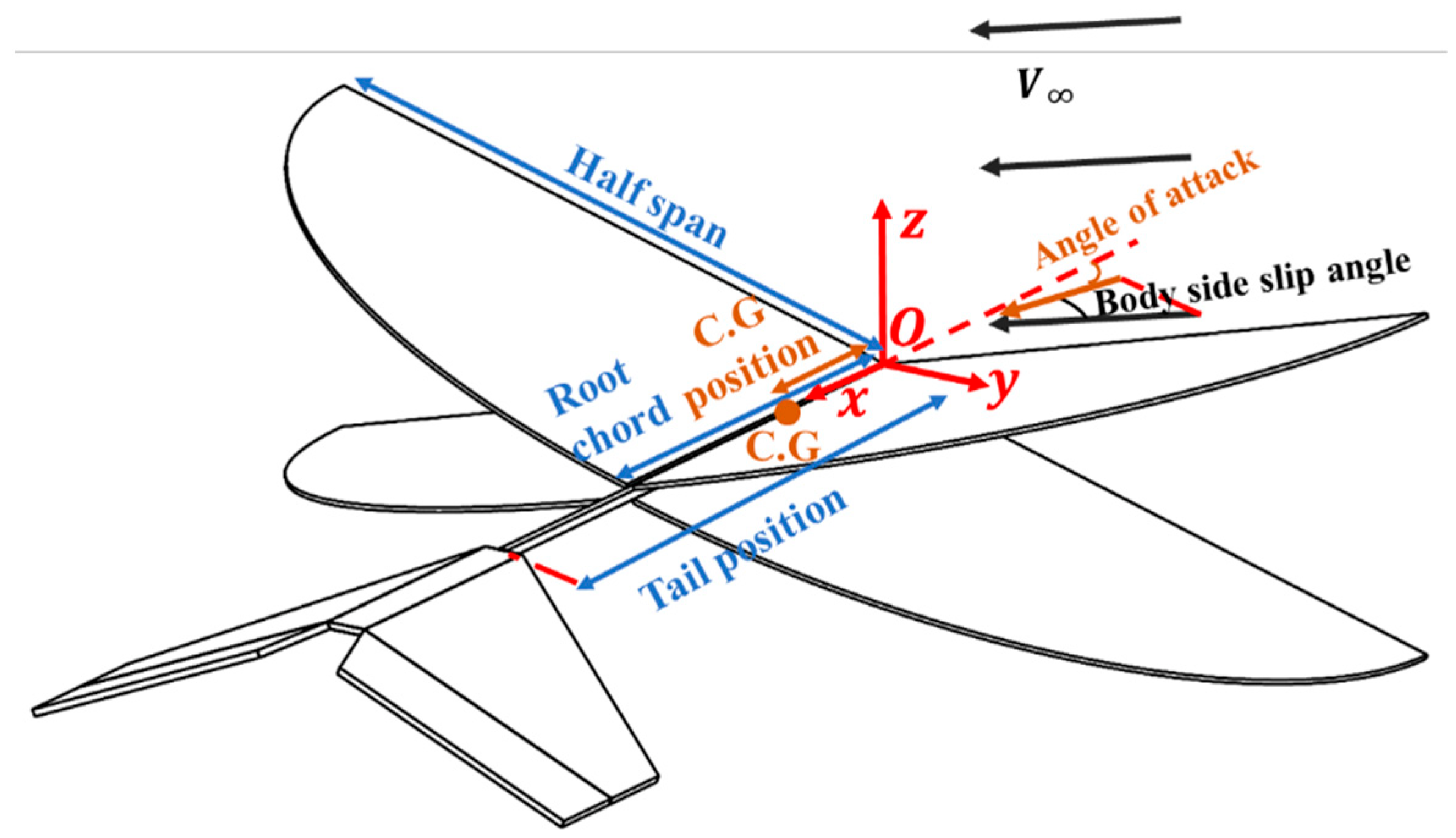
Coordinate system and parameters defined.

Figure 4.
Tail models in the simulation. (a) Undeflected and deflected tail control surfaces. (b) Inverted V–tail models with different dihedral angles.
Figure 4.
Tail models in the simulation. (a) Undeflected and deflected tail control surfaces. (b) Inverted V–tail models with different dihedral angles.

Figure 5.
Flexible deformation of wing.

Figure 6.
The surface deformation during flapping.

Figure 7.
Computational grids. (a) Initial computational grid. (b) Automatically remeshing computational grid.
Figure 7.
Computational grids. (a) Initial computational grid. (b) Automatically remeshing computational grid.

Figure 8.
Periodic change curve of torsion angle in 0.71 span.

Figure 9.
Comparison of simulated thrust and experimental thrust.

Figure 10.
Comparison of different types of time steps and grid numbers. (a) Lift comparison. (b) Drag comparison.
Figure 10.
Comparison of different types of time steps and grid numbers. (a) Lift comparison. (b) Drag comparison.

Figure 11.
Flapping wing vehicle force characteristics. (a) Lift coefficient curve. (b) Drag coefficient curve.
Figure 11.
Flapping wing vehicle force characteristics. (a) Lift coefficient curve. (b) Drag coefficient curve.

Figure 12.
Tails’ force characteristics. (a) Lift coefficient curve. (b) Drag coefficient curve. (c) L/D ratio.
Figure 12.
Tails’ force characteristics. (a) Lift coefficient curve. (b) Drag coefficient curve. (c) L/D ratio.

Figure 13.
Moment coefficient at different angles of attack on tails. (a) Pitch moment coefficient. (b) Yaw moment coefficient. (c) Roll moment coefficient.
Figure 13.
Moment coefficient at different angles of attack on tails. (a) Pitch moment coefficient. (b) Yaw moment coefficient. (c) Roll moment coefficient.

Figure 14.
Moment coefficient at different flow velocities. (a) Pitch moment coefficient. (b) Yaw moment coefficient.
Figure 14.
Moment coefficient at different flow velocities. (a) Pitch moment coefficient. (b) Yaw moment coefficient.

Figure 15.
Pressure center and aerodynamic center move with the angle of attack. (a) Pressure center position. (b) Aerodynamic center position.
Figure 15.
Pressure center and aerodynamic center move with the angle of attack. (a) Pressure center position. (b) Aerodynamic center position.

Figure 16.
The longitudinal moment coefficient with angle of attack.

Figure 17.
The lateral moment coefficient with body side-slip angle. (a) Yaw moment coefficient. (b) Roll moment coefficient.
Figure 17.
The lateral moment coefficient with body side-slip angle. (a) Yaw moment coefficient. (b) Roll moment coefficient.

Figure 18.
The relationship between tail position and control moment.

Figure 19.
The momenty time history of inverted T-tail.

Figure 20.
The relationship between the tail yaw restoring moment and body side-slip angle.

Figure 21.
Vorticity and streamlines in the section of y = 0.15 span with the inverted T-tail.

Figure 22.
Vorticity and streamlines in the section of y = 0.15 span with the inverted V-tail.

Figure 23.
The pitch moment changes of the inverted V-tail.

Figure 24.
Z-velocity distribution in the section of y = 0.175 span.

Figure 25.
X-velocity distribution in the section of y = 0.175 span.


Table 1.
Flapping wings parameters.
| Parameters | Data |
|---|---|
| Half span/cm | 14 |
| Root chord/cm | 10 |
| Area/cm2 | 426.4 (106.6 × 4) |
| Total stroke amplitude Φ/deg | 72 |
| C.G position/cm | 3.15 |
| Flapping frequency/Hz | 12.5 |
Table 2.
Tail design parameters.
| Parameters | Inverted T-Tail | Inverted V-Tail |
|---|---|---|
| Horizontal projection area | 73.74 cm2 | 73.74 cm2 |
| Vertical projection area | 28.93 cm2 | 28.93 cm2 |
| Total area | 137.26 cm2 | 81.25 cm2 |
| Weight | 1.8 g | 1.6 g |
Table 3.
Averaged thrust in time-convergence and grid-convergence tests.
| Type | Grid Number | Time Step Size (s) | Averaged Thrust (N) | Averaged Lift (N) |
|---|---|---|---|---|
| 1 | 823,035 | 0.0002 | −0.0424 | 0.1967 |
| 2 | 1,527,842 | 0.0002 | −0.0391 | 0.2027 |
| 3 | 3,145,743 | 0.0002 | −0.0386 | 0.2031 |
| 4 | 1,527,842 | 0.0004 | −0.0385 | 0.2034 |
| 5 | 1,527,842 | 0.0001 | −0.039 | 0.2029 |
Table 4.
Simulation conditions and research objectives.
| Section | Objective | Function | Variables | Control Surfaces‘ Deflection Angle |
|---|---|---|---|---|
| Section 3.1.1 | Aerodynamic forces of wings and tail | Lift Drag L/D ratio | Angle of attack [0°, 5°, 10°, 15°, 20°, 30°, 40°, 50°, 60°] | 0° |
| Section 3.1.2 | Control moment of tails | Cmx Cmy Cmz | Angle of attack [0°, 5°, 10°, 15°, 20°, 30°, 40°, 50°, 60°] Velocity [0 m/s, 2 m/s, 4 m/s, 6 m/s, 8 m/s, 10 m/s] | 45° |
| Section 3.1.3 | Longitudinal static stability of tails | Cmy Pressure center Aerodynamic center | Angle of attack [0°, 5°, 10°, 15°, 20°, 30°, 40°, 50°] | 0° |
| Section 3.1.4 | Lateral static stability of tails | Cmx Cmz | Body side-slip angle [0°, 2.5°, 5°, 10°, 12.5°, 15°] | 0° |
| Section 3.2.1 | Effect of tail position | Pith control momentYaw control moment | Tail position [11.5 cm, 13 cm, 14.5 cm, 16 cm, 17.5 cm] | 45° |
| Section 3.2.2 | Effect of V-tail dihedral angle | Directional static stability | [22.5°, 30°, 37.5°, 45°, 52.5°] | 0° |
Publisher’s Note: MDPI stays neutral with regard to jurisdictional claims in published maps and institutional affiliations. |
© 2022 by the authors. Licensee MDPI, Basel, Switzerland. This article is an open access article distributed under the terms and conditions of the Creative Commons Attribution (CC BY) license (https://creativecommons.org/licenses/by/4.0/).
Share and Cite
MDPI and ACS Style
Li, H.; Li, D.; Shen, T.; Bie, D.; Kan, Z. Numerical Analysis on the Aerodynamic Characteristics of an X-wing Flapping Vehicle with Various Tails. Aerospace 2022, 9, 440. https://doi.org/10.3390/aerospace9080440
AMA Style
Li H, Li D, Shen T, Bie D, Kan Z. Numerical Analysis on the Aerodynamic Characteristics of an X-wing Flapping Vehicle with Various Tails. Aerospace. 2022; 9(8):440. https://doi.org/10.3390/aerospace9080440
Chicago/Turabian StyleLi, Huadong, Daochun Li, Tong Shen, Dawei Bie, and Zi Kan. 2022. "Numerical Analysis on the Aerodynamic Characteristics of an X-wing Flapping Vehicle with Various Tails" Aerospace 9, no. 8: 440. https://doi.org/10.3390/aerospace9080440
Note that from the first issue of 2016, this journal uses article numbers instead of page numbers. See further details here.