
Flight Departure Time Prediction Based on Deep Learning


Department of Traffic and Transportation, Nanjing University of Aeronautics and Astronautics, Nanjing 210016, China
*
Author to whom correspondence should be addressed.
Aerospace 2022, 9(7), 394; https://doi.org/10.3390/aerospace9070394
Submission received: 25 May 2022
/
Revised: 9 July 2022
/
Accepted: 11 July 2022
/
Published: 21 July 2022
(This article belongs to the Section Air Traffic and Transportation)
Abstract
:Accurate flight departure time prediction enables the rational use of airport support resources, aprons, and runway resources, and promotes the implementation of collaborative decision-making. In order to accurately predict the flight departure time, this paper proposes a deep learning-based flight departure time prediction model. First, this paper analyzes the influence of different factors on flight departure time and the influencing factor. Secondly, this paper establishes a gated recurrent unit (GRU) model, considers the impact of different hyperparameters on network performance, and determines the optimal hyperparameter combination through parameter tuning. Finally, the model verification and comparative analysis are carried out using the real flight data of ZSNJ. The evaluation values of the established model are as follows: root mean square error (RMSE) value is 0.42, mean absolute percentage error (MAPE) value is 6.07, and mean absolute error (MAE) value is 0.3. Compared with other delay prediction models, the model established in this paper has a 16% reduction in RMSE, 34% reduction in MAPE, and 86% reduction in MAE. The model has high prediction accuracy, which can provide a reliable basis for the implementation of airport scheduling and collaborative decision-making.
1. Introduction
According to the data provided by the Civil Aviation Administration of China (CAAC), it can be seen that when China was affected by COVID-19 in 2020, China’s total civil aviation passenger transport was only 79.83 billion ton-kilometers. However, from 2016 to 2019, China’s total civil aviation passenger transport has grown from 96.25 billion ton-kilometers in 2016 to 129.33 billion ton-kilometers in 2019 [1]. Additionally, the International Air Transport Association (IATA) predicts that by 2035, the total number of passengers worldwide will reach 720 million, tripling compared to 2016 [2]. These data show that the civil aviation industry in China and even the world is developing rapidly, and the total passenger volume of civil aviation has risen sharply. The increase in civil aviation transportation demand will lead to a larger number of flights. Flight operations will need to occupy the support resources, apron resources, and runway resources in the airport. The contradiction between the increasing flight demand and the lack of resources can easily affect flight operations and cause delays. Therefore, studying the factors affecting flight departures and predicting flight departure times contribute to utilizing the limited resources in the airport reasonably, and implementing the collaborative decision-making mechanism.
In recent years, scholars have performed a lot of research on delay prediction. Most studies work as follows: firstly, they analyzed and screened the factors that may cause flight delays. Then, they built a delay prediction model and finally used machine learning [3,4,5,6,7,8,9,10,11,12] or deep learning [13,14,15,16,17,18,19,20,21,22,23,24,25] algorithms to solve the problem. Similarly, they used ensemble learning [26].
Machine learning is widely used in flight delay prediction due to its understandability and ease of use. B [3] et al. obtained general flight information, track point information, and weather information from different sources, and then established a random forest model and a deep neural network to predict the aircraft planned arrival time. The mean absolute error (MAE) of the prediction results were all less than 6 min. G [4] et al. combined basic flight information such as ICAO identification number, location, airport weather information, and traffic flow information into a comprehensive dataset. Then, considering the long short-term memory (LSTM) network is prone to over-fitting in limited data sets, the random forest model was used to classify and predict flight delays, and the prediction accuracy achieved 90.2%, so as to avoid over-fitting. Zhen [5] et al. screened out factors such as airline size and actual aircraft capacity on multiple routes and made flight departure delay predictions by a hybrid method of random forest regression and maximal information coefficient (RFR-MIC). Wu [8] et al. considered factors affecting flight delays from airports, airlines, and aircraft, such as delay time, route, planned departure time, planned arrival airport, etc., and then used the principal component analysis method to reduce the dimension of the data. Finally, they obtained the final characteristic factors, including the planned arrival airport, planned departure time, etc. The prior knowledge of flight delay is added to the support vector machine (SVM) model in the form of inequality, and the improved SVM model is used for flight delay prediction. Zhang [11] et al. selected the month and distance from the flight records, selected factors such as wind speed and visibility from the weather data as the factors affecting flight delays, and then used the categorical boosting (CatBoost) algorithm to predict flight delays. In the end, they used Shapley additive explanation (SHAP) to analyze the contribution of factors. In order to improve the robustness of the boarding gate allocation scheme, Micha [12] et al. used mixed density network and random forest regression models to predict the delay distribution of departure and arrival flights. They have selected the influencing factors including airport, airline, aircraft type, etc.
Deep learning is a new research direction proposed in recent years based on machine learning. Due to its powerful data mining and processing power, deep learning is also widely used in flight delay prediction. Desmond [13] et al. proposed social ski driver conditional autoregressive-based (SSDCA-based) deep learning. The factors that affect flight delay are considered as flight date, departure airport, arrival airport, departure delay, arrival delay and distance. Finally, the above optimization algorithm is combined with the deep LSTM neural network to predict the flight delay classification. The prediction result of root mean square error (RMSE) is 0.1113 and mean square error (MSE) is 0.0124. Cai [14] et al. started from multi-airport scenarios, considering that delay time series and time-evolving graph structure cannot be directly used as network input, so they proposed a temporal convolution block and an adaptive graph convolution block based on Markov features to solve the flight delay problem. Jiang [15] et al. established a multi-input and output LSTM time series, prediction model. The input factors are planned departure time, planned arrival time, flight attributes, etc. The output factors are flight delay rate, average delay time, and other indicators for evaluating delays. At the same time, by changing the length of the time window, the optimal length to improve the prediction accuracy is determined. Li [16] et al. selected the actual number of inbound flights, the actual number of departure flights, and the departure delay time as factors affecting flight delays, and made a classification prediction of flight delays by establishing an LSTM neural network. Qu [17] et al. constructed a new fusion dataset by fusing flight data and meteorological data, and then classified and predicted flight delays by building a deep convolutional neural network. Shi [21] et al. first determined the centroid of flight delay classification by k-means clustering, then used the grey correlation degree to filter factors. The factors they have selected include delay time of departure, planned arrival time, wind speed, rainfall, etc. Finally, the genetic algorithm was used to optimize the parameters of the BP neural network, and the combined model was used to classify and predict the flight delay problem. Wang [22] et al. divided the factors that affect flight delays into direct factors and indirect factors. The direct factors include the number of passengers, airport congestion, aircraft size, etc. Additionally, the indirect factors include the location of the departure airport and the operation of previous flights, etc. LSTM neural network based on force mechanism for flight delay prediction.
In recent years, scholars have focused more on delay prediction than departure time prediction, so few articles study flight departure time prediction. Delay prediction is to predict the specific delay time of the inbound and outbound flights that have been delayed, and its purpose is to give early warning of flight delays and reduce the possibility of delays. Many factors can easily affect flight delays. Additionally, the delay formation mechanism is complex. It is the reason why it is difficult to obtain specific data on the actual influencing factors. High model complexity and difficulty in data acquisition make it impossible to establish a reasonable delay prediction model. Flight departure prediction is used to predict the specific departure time of the flight. By screening the factors closely related to the flight departure, the regression prediction of the actual flight departure from the planned departure time is carried out. Departure time prediction does not need to consider many factors, and the specific flights can be focused on. Therefore, a flight departure time prediction model is proposed to screen the influencing factors, reduce the modeling complexity, and finally obtain an accurate flight departure time, which can provide a reliable basis for airport scheduling and the implementation of collaborative decision-making systems.
First, this paper summarizes the factors affecting flight operation in existing research results, and analyzes and filters the factors, so as to determine the factors affecting flight operation. Then, the GRU neural network model is established, which is verified by the real flight data. Finally, compared with several commonly used neural network models and random forest models in machine learning, the advantages of the model built in this paper are highlighted.
2. Flight Departure Time Prediction Modelling
In this section, this paper first summarizes the factors affecting flight departures mentioned in the literature review, analyzes the impact of these factors on flight departures, and identifies these influencing factors. Then, considering the different dimensions between various factors, this paper has chosen the appropriate method to deal with it. Finally, this paper proposes a departure flight prediction model and records the parameter tuning process.
2.1. Factors Selection
Summarizing the influencing factors mentioned in the literature review, this paper found that the factors affecting flight operation can be mainly divided into three categories: flight information factors, airport factors, and weather factors. The classification results are shown in Table 1 below.
Different types of factors have disparate effects on flight operation. The factors analyzed by this paper can be summarized as:
- 1.
- Flight Information Factor
The flight information factor records basic flight operations. For example, the planned and actual departure time of a departure flight with a previous flight characterizes the basic operating rules of this flight. This paper takes the actual departure time as the research object of this paper, which can more accurately reflect the actual operation law of the studied flight. At the same time, the planned and actual landing time of the previous flight is the characterization of the operation of the previous flight, which will affect the actual departure time of the next flight, so this paper considers it as one of the influencing factors.
- 2.
- Airport Factor
The airport is the meeting point that provides all the resources for flight departure, and it is also the gathering place for different stakeholders. The weather conditions and geographical location of the airport may affect the take-off and landing of flights. If a large number of flights need to take off and land within the time period of the departing flight, the departing flight needs to wait for other flights, so the departure time may be disturbed. Therefore, the number of flights taking off and landing at the airport is also one of the factors considered in this paper.
- 3.
- Weather Factor
Weather factors mainly consider the weather changes in the atmosphere, including temperature, humidity, visibility, and cloud thickness. Weather factors will change flight take-off and landing conditions and affect flight operational safety. For example, when the temperature is too low, the flight will be confronted with the risk of the ground icing, which will cause a long break distance due to the reduction of friction during the taxiing process.
- 4.
- Airline Factor
As one of the stakeholders, the airline will have a certain impact on the flight operation. For example, the equipment configuration, personnel arrangement, and company size of the airline will affect the specific departure time of the flight, resulting in fluctuations in the actual departure time. Generally speaking, large airlines have more reasonable equipment allocation than small airlines and have more large aircraft. However, most of the current literature does not consider this aspect, which may be due to the difficulty in obtaining relevant data or quantifying such data. However, we cannot deny that airlines will also have a certain impact on flight operations.
To sum up, in terms of flight information factors, the deviation between the previous flight plan and the actual landing time is selected as the influencing factors, and the deviation between the departure flight plan and the actual departure time is selected as the research object. In terms of airport factors, two factors are selected: the number of departures and the number of landings within the time period to be predicted. According to the current development of civil aviation technology, when the flight operates, if there is no extreme weather, the flight will not be delayed due to general weather, or the actual departure time will not deviate significantly from the planned time. Therefore, no consideration is given to the weather factor. At the same time, the flight departure time has a certain sequence, so the month is selected as one of the influencing factors. The description and value range of each feature is shown in Table 2.
2.2. Data Preprocessing
Firstly, the specific information of the corresponding flight by the flight number can be found in the original data set. Then, the missing data would be deleted. Most of the flight delay classification prediction literature classifies delays with flight delays less than 60 min as mild delays. We believe that adding mild delay data into the data set will not cause noise interference and can improve the robustness of the model. Therefore, the flight data in which the actual departure time deviates from the planned time by more than one hour will be deleted. Finally, data are composed according to the data type described in Section 2.1.
In this paper, multiple factors are selected for modeling, and the properties of each factor are different, with disparate dimensions and orders of magnitude. In order to unify the dimensions between the factors and avoid the gradient explosion problem during neural network training, it is necessary to normalize the factors. Common normalization methods include min–max normalization and Z-score normalization. This paper uses the min–max scaling maximum and minimum normalization method in the SK-learn library that comes with Python3.7 and SK-learn 0.24.2. The formula is as follows:
The min–max scaling method can achieve equal scaling of the original data. The scale is determined by the maximum and minimum values in the data, and the data can be scaled to the range of [0, 1] or [−1, 1]. Therefore, the maximum and minimum normalization method is used for data processing.
2.3. Building a GRU Neural Network Prediction Model
2.3.1. Theoretical Knowledge
In the past few years, standard machine learning and its proposed variants have been able to achieve relatively satisfactory results in different fields. However, such methods are usually constrained to hand-crafted features and limited capacity for learning intrinsic patterns in data. In this context, scholars have proposed a deep learning-based approach. Deep learning is mostly used to deal with image, video data, and sequence problems, and can have a good performance in other fields. Among them, the most popular deep learning method for dealing with sequence problems is the recurrent neural network (RNN) [27].
However, when the input sequence data are too long, it is difficult for standard RNNs to preserve historical information from decision points [28]. That is to say, when the data sequence is too long, the network tends to forget the learned historical data features and over-learn the current data features, that is, the phenomenon of gradient disappearance occurs. The proposal of LSTM solves the problem that standard RNN is prone to gradient disappearance when faced with long sequence data.
The LSTM was first implemented in 1997 by Hochreiter and Schmidhuber, where the main objective was to improve results on long sequences of data [29]. Its working principle is similar to traditional RNN, that is, the input of the current neuron depends on the cyclic information of the output of the previous neuron. Unlike RNN, LSTM has a more complex architecture. LSTM controls the retention and deletion of data information through three gates, namely forget gate, input gate, and output gate. The forgetting gate is used to control the retention and deletion of information. The input gate receives the information retained by the forgetting gate and the input information of the current state and then passes it to the output gate after being activated by the activation function. The output gate is responsible for the final output of the network.
LSTM has been able to process and learn sequence data very well. However, considering the complex internal structure and difficult-to-control learning mechanism of LSTM, GRU is proposed on the basis of LSTM. GRU was originally used to improve results in the neural machine translation [27]. Unlike LSTM, GRU combines the forget gate and the input gate into a single update gate and mixes neurons and hidden states to reduce network parameters and improve the training speed [30].
The GRU neural network relies on the following four formulas for feature extraction in the original data:
In the formula, is the current time input, is the hidden state of the previous moment, and is the hidden state computed at the moment. Equation (2) is the calculation method for the value of the reset gate , is the hidden state of the reset gate layer, and is the sigmoid activation function. Equation (3) is used to calculate the hidden state . Equation (4) is used to calculate the value of the update gate, which is used to control how much information the previous hidden state can be transmitted to the current hidden state. Equation (5) finally calculates the current hidden state, and the hidden state enters the next layer of neurons with the input of the next layer.
2.3.2. Model Establishment and Parameter Tuning
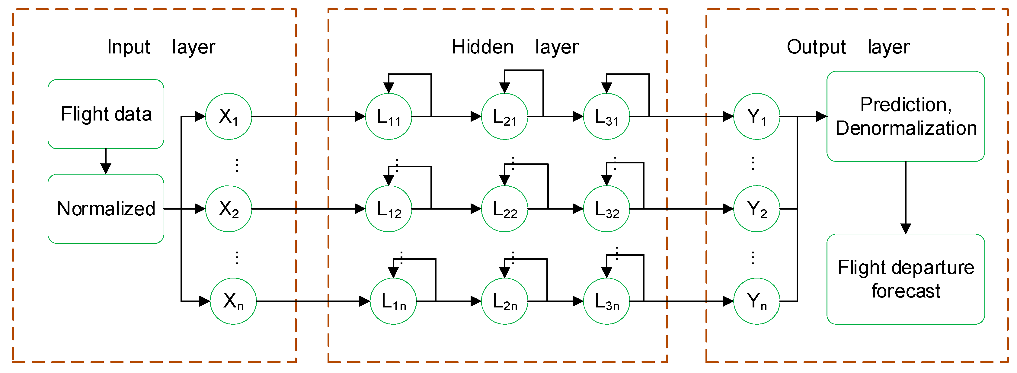
This article is based on Python3.7 and Keras2.2 framework for model building. A schematic diagram of the model is shown in Figure 1.
Neural networks contain a large number of hyperparameters, such as the number of neurons, iterations, batch size, etc. Various hyperparameters have different effects on network performance. For example, the number of iterations determines the learning ability of the neural network, and the batch size setting determines whether the model can converge and find the global optimum. Different hyperparameters can generate different combinations. Due to the limited space of this paper, this paper only shows the tuning process of the two hyperparameters, the batch size, and the number of neurons in the hidden layer.
In this paper, three evaluation functions are selected to evaluate the proposed forecasting model: RMSE, MAE, and MAPE. The three evaluation function formulas are given by:
RMSE is the square root of the squared sum of the deviation of the predicted value from the actual value and the ratio of the number of predictions, which can be used to measure the deviation between the predicted value and the actual value. MAE is the absolute value of the deviation of all individual predicted values from the arithmetic mean, avoiding the phenomenon of cancellation between predicted and true values. MAPE is used to reflect the degree of deviation of each predicted value from the true value. These three evaluation indicators are used to evaluate the quality of the model. A higher evaluation value indicates that the model fitting effect is poor. Instead, a low evaluation value indicates that the model fitting effect is perfect.
First of all, it is determined that the GRU network-based departure flight prediction model proposed in this paper adopts a GRU network structure with three hidden layers. The learning rate adjustment method is an adaptive learning rate adjustment algorithm (Adam). The number of iterations is set to 300. The changes in the model are observed by controlling two parameters, the number of hidden layer nodes and the batch size. When changing the number of hidden layer nodes, the batch size is set to 32; when changing different batch sizes, the number of hidden layer nodes is 50. The result is shown in Table 3 and Table 4.
It can be seen from the above comparison experiments that the model effect is the best when the number of neurons in the hidden layer of the model is 50 and the batch size is set to 32.
3. Case Analysis
In this section, this paper first describes the dataset, which is divided into the training set, test set, and validation set to facilitate the training and validation of the model. Then, this paper observes the error curves and prediction performance on the training and validation sets. In order to prevent the model from overfitting, an early stopping strategy is used. Compared with the model without an early stopping strategy, it proves that an early stopping strategy can avoid the phenomenon of model overfitting. Finally, compared with the commonly used neural network models and non-neural network models, the superiority of the model proposed in this paper is highlighted.
3.1. Data Description
This paper uses the actual flight operation data of Nanjing Lukou International Airport (ICAO airport code: ZSNJ) from January 2019 to December 2020. ZSNJ is one of the busiest civil airports in China and is the primary airport serving Nanjing. The relevant data are obtained through the flight schedule provided by the airport. The original data set has 100,000 flight records, each record includes flight attributes, flight number, route, planned arrival (departure) time, actual arrival (departure) time, aircraft type, and aircraft number. Because there will be flight cancellations and serious delays during the actual flight operation, and at the same time, this paper studies the changing trend of the departure time of a single flight. Therefore, after the processing in Section 2.2, each flight has between 400 and 500 operational records. Compared with the 63,460 flight records used by B et al. [3], the dataset used in this paper is large in size.
3.1.1. Training Set
The core part of the dataset is the training set. The training set presents the scale of flight operations and the characteristics of data changes. The size of the training set affects the learning effect of the model. If the training set is too large, then it contains a large amount of data, takes a long time to train, and is prone to noisy data. If the training set is too small, then it is difficult to fully present the characteristics of data changes, but the training time is short. By consulting relevant information, we set the flight records owned by the training set to account for 80% of the total data set, and the data volume ranges from 320 flight records to 400.
3.1.2. Test Set
After model training, a corresponding proportion of the test set needs to be set for parameter tuning and to determine whether the model can learn data features. In the Keras framework, the test set can be automatically divided into the training set through the proportional division function for testing. The test set data participates in the training process in order to prove that the model can learn the data features contained in the training set. The test set accounts for 20% of the total data set, and the data volume is between 80 flight records and 100.
3.1.3. Validation Set
The validation set is used to verify the performance of the model. After the model is trained and tested on the training set and the test set, it can ensure that the model has learned the data features contained in the training set. However, if the model overfits and overlearns the features of the training set, it will reduce the transferability of the model. Therefore, the transferability of the model is evaluated using the validation set data that the model has never learned. The validation set also accounts for 20% of the total data set, and the data volume is between 80 flight records and 100.
In summary, various set ratio settings conform to the law of 6:2:2. Model training and testing are performed on the datasets with such proportions, and the results are as follows.
3.2. Prediction Result Display
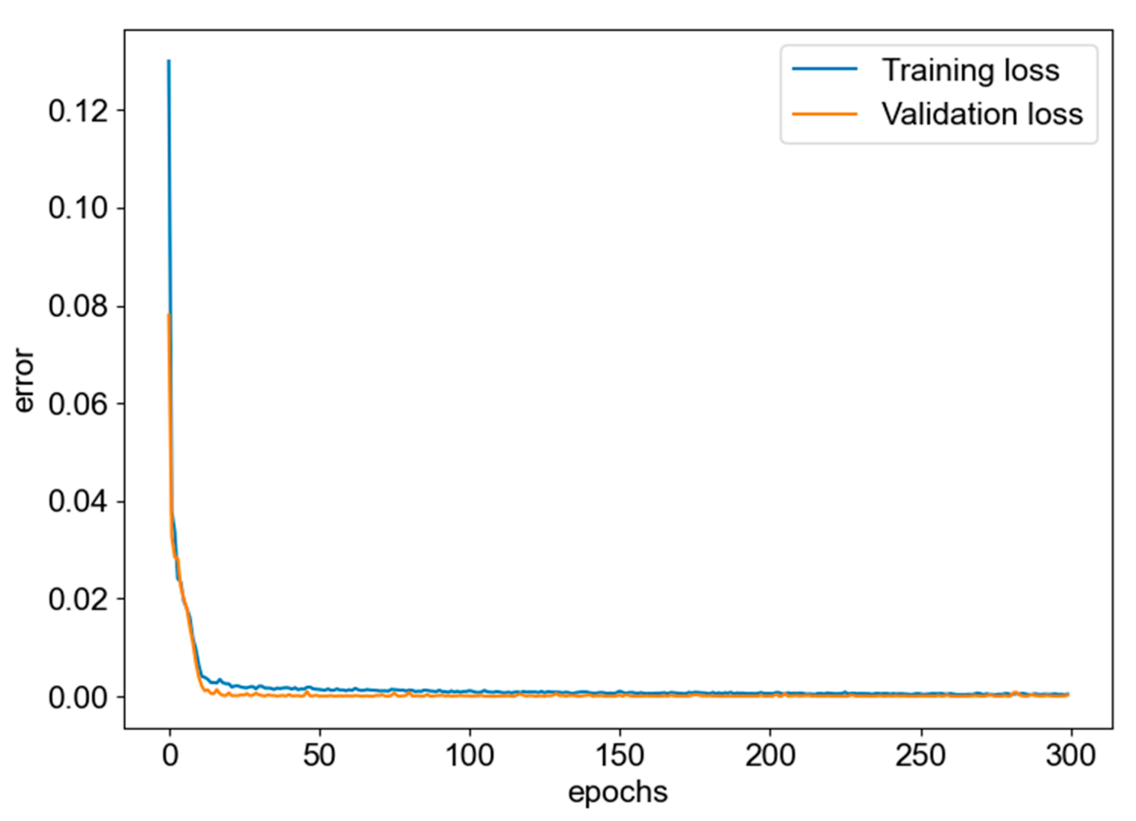
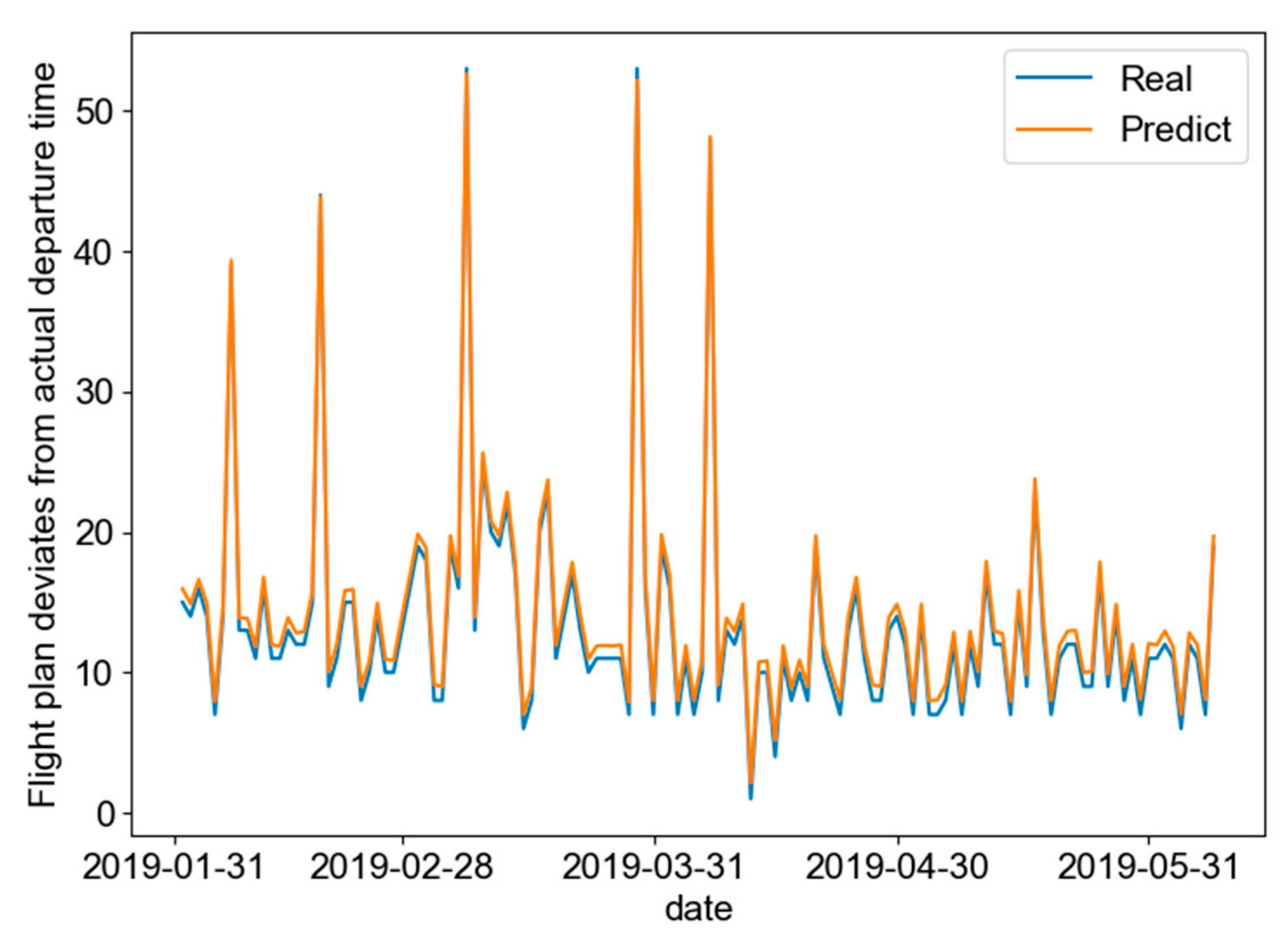
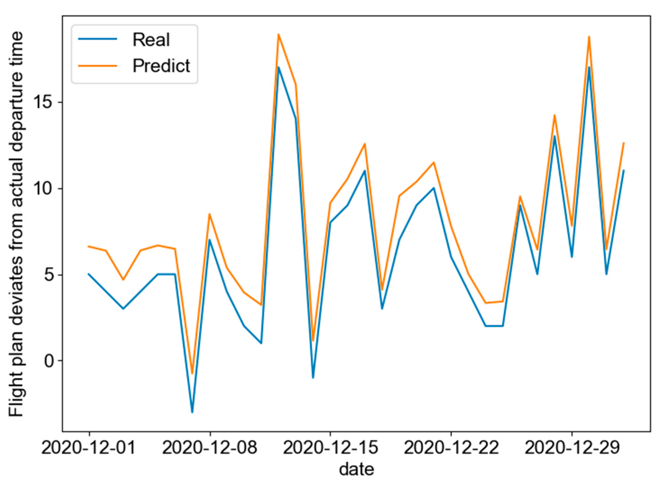
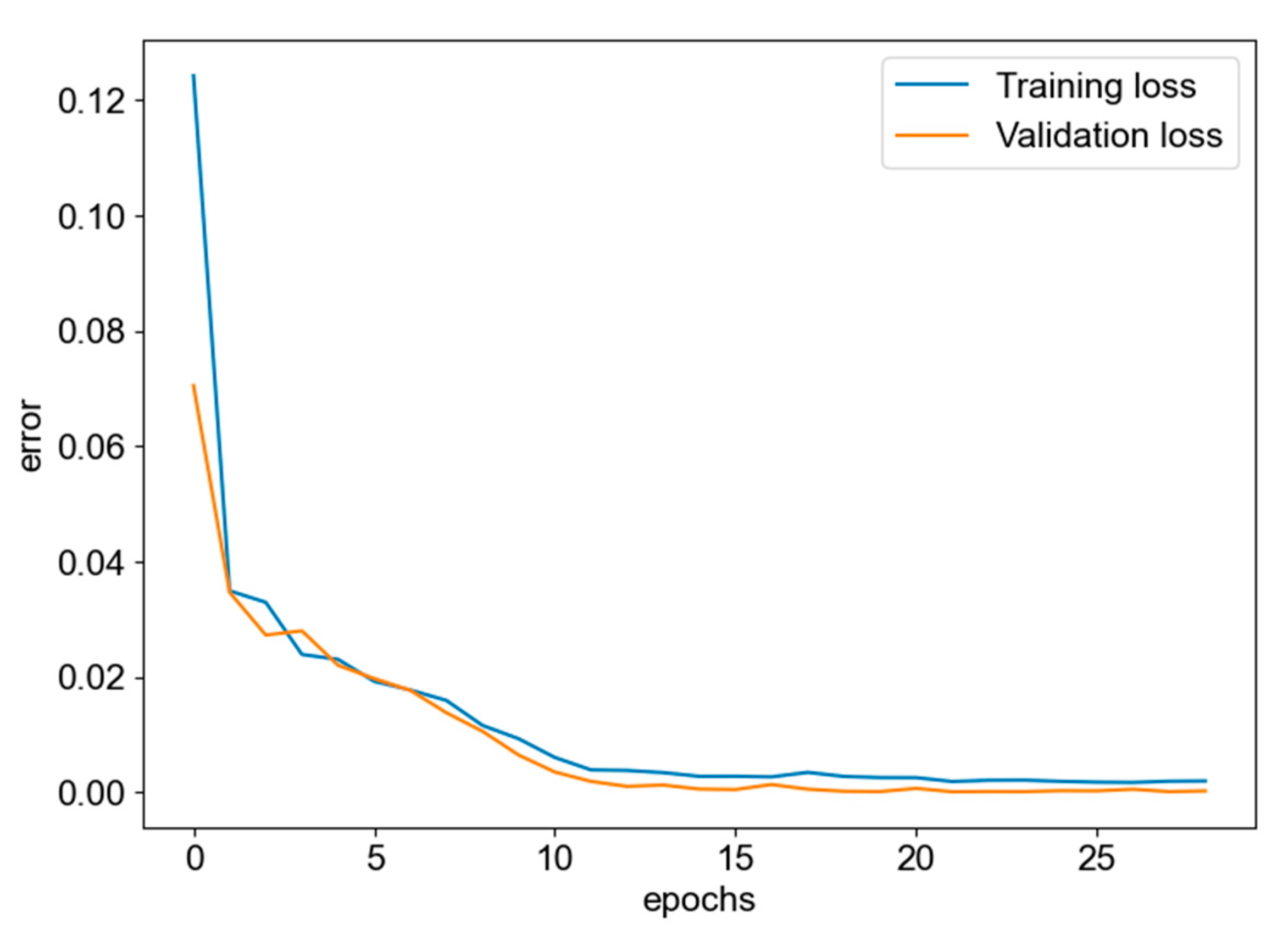
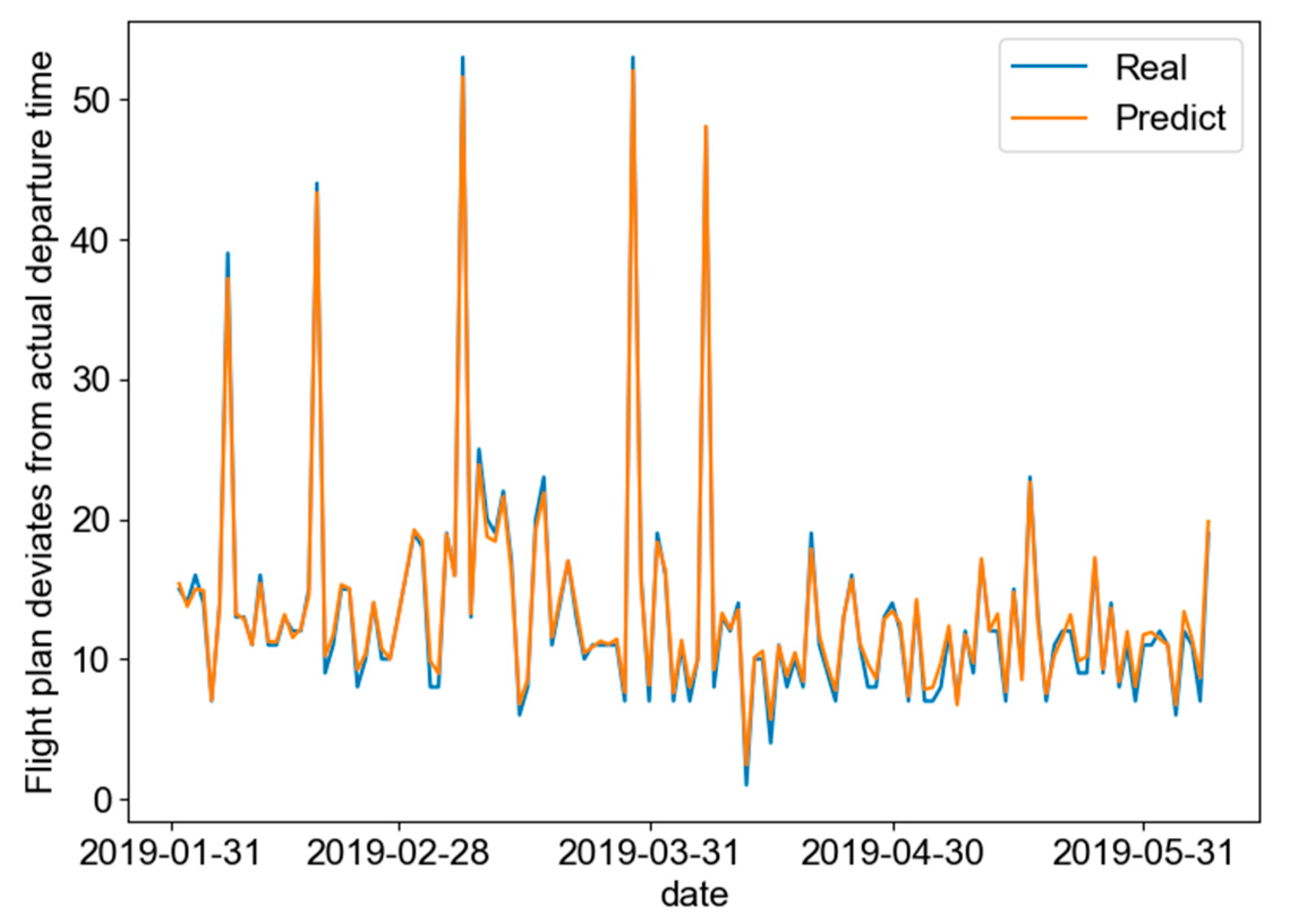
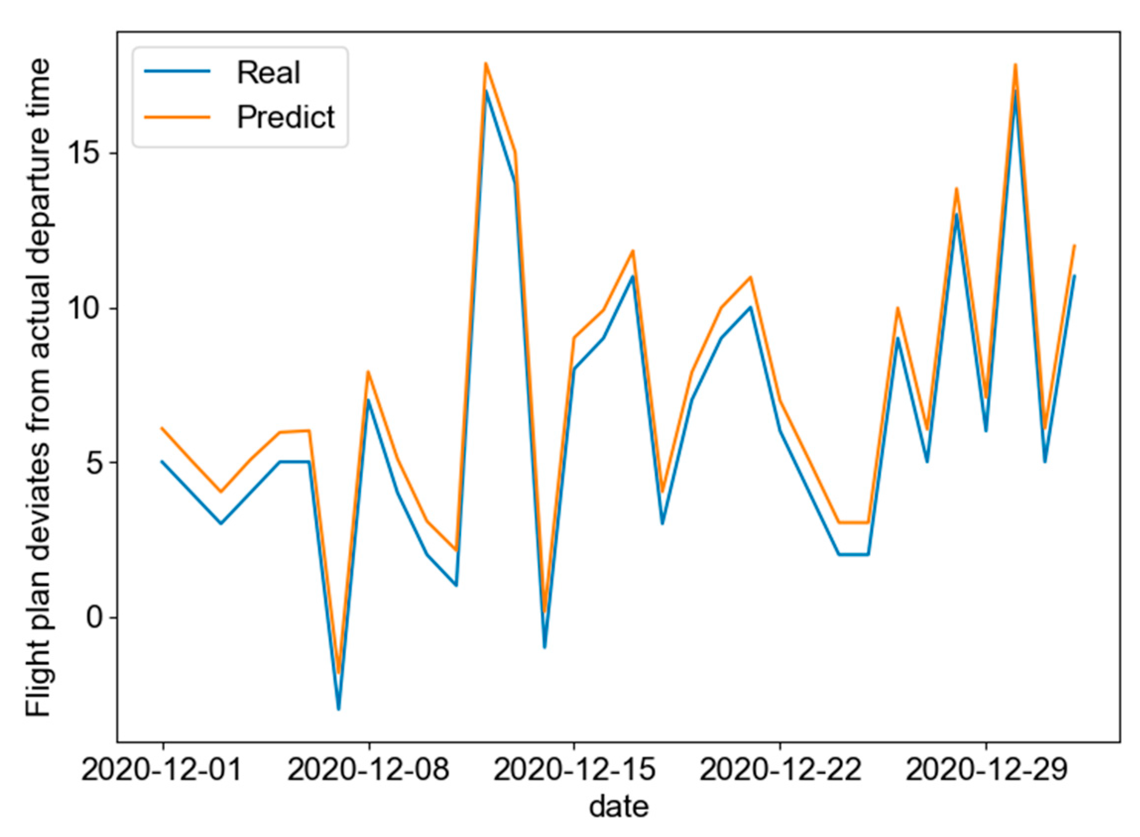
By observing the error curve of the training set and the test set, we can understand the trend of error change. Visualize the fitting effect of the training set and validation set data to determine whether the model has learned the characteristics of the data set and whether it has converged. First, this paper uses the flight data of the flight number AQ1033 in ZSNJ to conduct the test, the error curve is shown in Figure 2. The fitting effect of the training set data is shown in Figure 3. The fitting effect of the validation set data is shown in Figure 4.
The error curve shows that the error gradually decreases at the beginning. Additionally, as the number of iterations increases, the error gradually converges to a fixed value and does not change anymore. The fit plots in Figure 3 and Figure 4 show the model’s performance on the training set and validation set, respectively. However, as can be seen from the graph, the error hardly changes when the training progresses to around 50 iterations. Therefore, in order to prevent the model from overfitting, a certain early stopping strategy is adopted. By setting a certain test set error threshold, when the error is less than the threshold, the model stops iterating. If the threshold is set too high, the model does not fully learn all the features. If the threshold is set too low, the model prefers to learn individual features and ignores global features. After a number of trials, the model stopped iterating when the threshold was determined to be 0.0006. Figure 5, Figure 6 and Figure 7 show the error curve and the fitting diagrams of the training set and validation set after using the early stopping strategy.
It can be seen from the above experiments that after adding the early stopping strategy, the model has an obvious improvement on the validation set, indicating that the model can improve certain over-fitting phenomenon after adding the early stopping strategy. Additionally, this model can learn the characteristics of the training set and be applied to the validation set. The RMSE value in this AQ1033 flight data experiment is 0.42, the MAPE value is 4.07, and the MAE value is 0.3.
Then, the domestic flight data of different time periods are selected to verify the applicability of the model, and the evaluation function values corresponding to each flight data are shown in Table 5 below.
As can be seen from the table, the performance of the model in different flight data is roughly the same as the performance of the AQ1033 flight data set, which verifies the applicability of the model.
3.3. Comparison and Analysis of Results
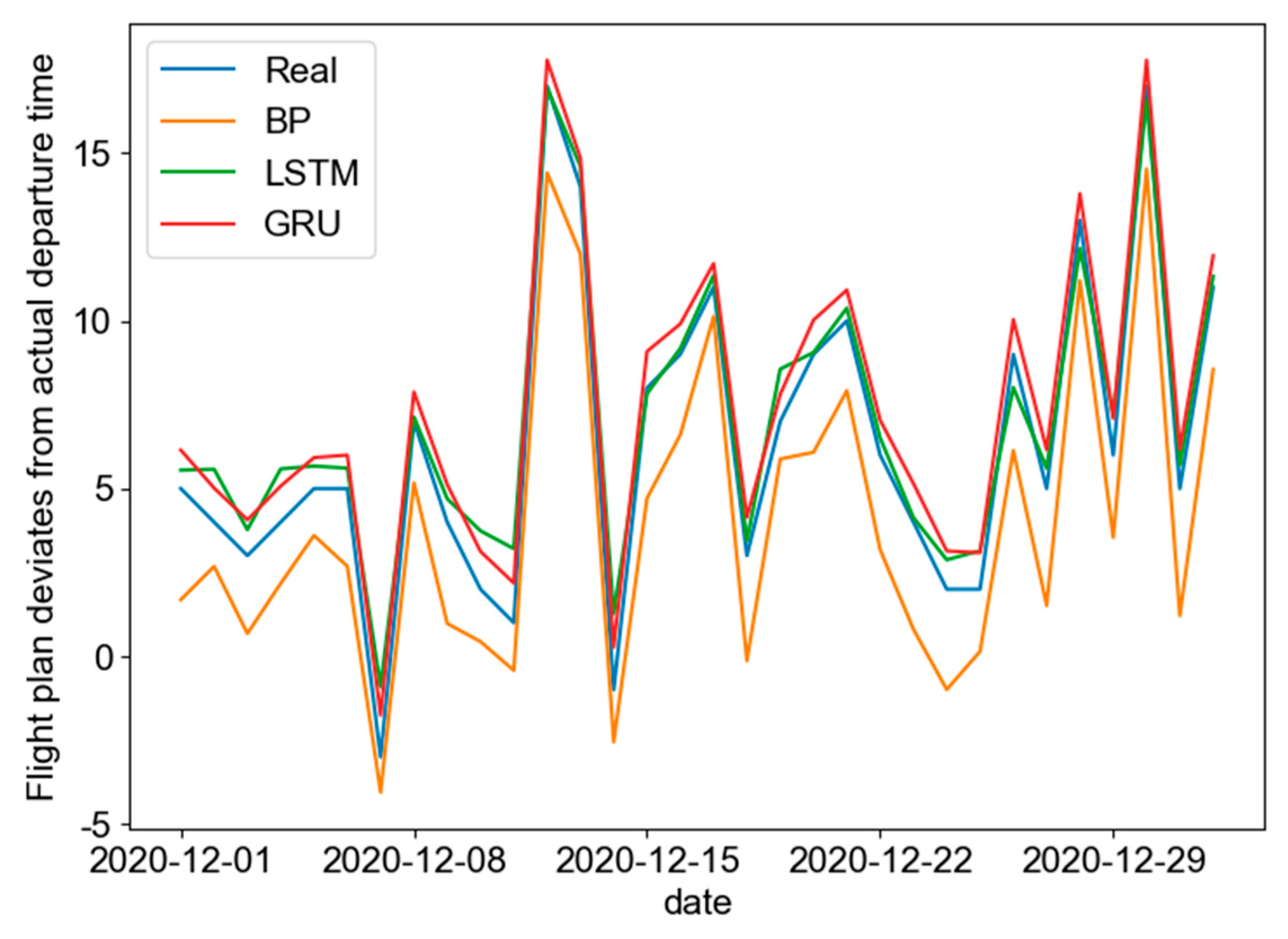
Compared with another two commonly used BP neural network models and LSTM neural network models, under the same AQ1033 flight data set, a comparison experiment of the fitting effects of the three models is carried out. The experimental results are shown in Table 6. The comparison of model fitting effect is shown in Figure 8.
It can be seen from the table that the evaluation function values of the LSTM neural network and the GRU neural network are roughly close, but the value of the GRU network is lower than that of the LSTM network, and the evaluation function value of the BP neural network is the highest. In the fitting diagram, it shows that LSTM and GRU neural networks not only can learn the trend of curve changes, but also can accurately fit each value. However, BP seems to be difficult to learn the trend of the curve change and the fitting effects of each value are also poor.
In their research, B [3] et al. proposed deep neural network and random forest models, which are the most commonly used and most representative models in flight operation forecasting.
3.3.1. Deep Neural Network (DNN)
A deep neural network means a neural network with multiple hidden layers [3]. Its principle is similar to BP neural network. BP neural network generally refers to a network with a single hidden layer, updating the weight matrix through the back-propagation algorithm, and then learning the characteristics of the training set. However, the weight matrix constructed by a single hidden layer is prone to under-fitting, which makes the model unable to learn the training set features well. Therefore, deep neural networks came into being. The deep neural network increases the number of hidden layers and expands the scale of the feature matrix to ensure that the features of the training set can be captured by the model without overfitting.
3.3.2. Random Forest (RF)
RF is an ensemble learning method to build a forest of uncorrelated decision trees using a procedure such as classification and regression trees (CART), with random split selection and bagging [3]. The decision tree has three types of nodes: root node, leaf node, and intermediate node. The root node represents the entire sample dataset, the leaf nodes correspond to the final decision result, and the intermediate nodes correspond to different feature attribute tests. A random forest is a combination of different decision trees, in order to solve the problem of the weak generalization ability of a single decision tree. Random forest votes on the training set features learned by different decision trees, selects the features with the highest scores for retention, and guides the model to make predictions.
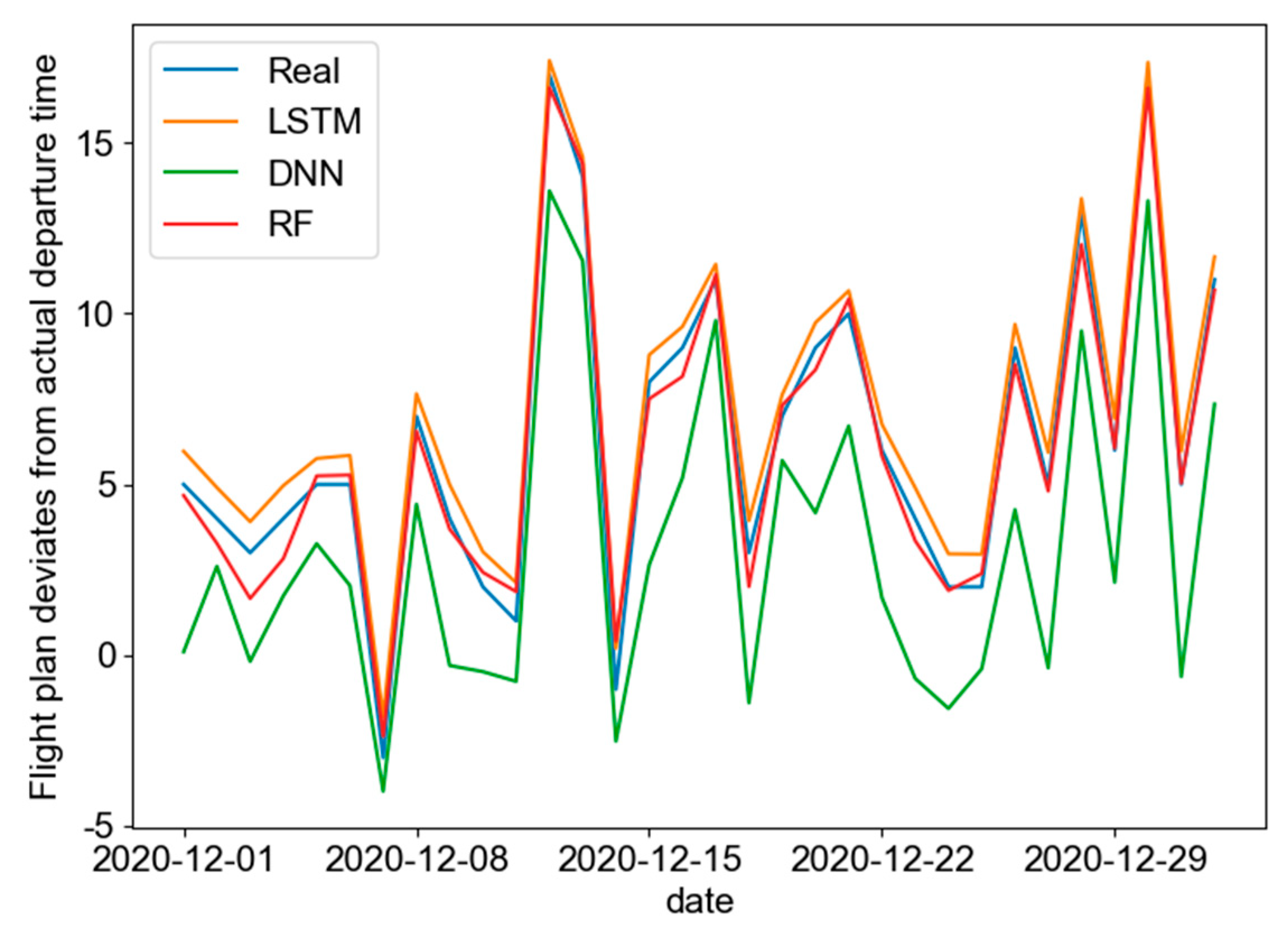
The comparison results of the model established in this paper and the above two classic models using the same data set and setting the same hyperparameters are shown in Table 7, and the fitting effect is shown in Figure 9.
Compared with the prediction model proposed above, the GRU neural network model established in this paper has the lowest value of the evaluation function and the best effect in terms of the numerical change trend. The evaluation index value RMSE is reduced by 16%, MAPE is reduced by 34%, and MAE is reduced by 82%, which can better illustrate the superiority of the established model.
In summary, the model proposed in this paper based on GRU neural network for flight departure time prediction has good applicability and practicability. GRU neural network performs well in accuracy and fitting trends and can accurately and reliably predict flight departure time.
4. Conclusions
Aiming at the problem of predicting the departure time of a single flight, this paper proposes a GRU neural network prediction model under the influence of multiple factors. The experimental results based on the test set show that the selected influencing factors are closely related to the flight operation. The model can learn the operation rules of the corresponding flight and use them to predict the operation situation of future flights. For different stakeholders, the model has different usage times and provides different reference values. For different stakeholders, the model is used during different times with different reference values. For example, airlines can use the model to predict the operation of their own flights, which is to analyze the reasons for the deviation between the planned time and the actual time, and to improve passenger satisfaction. For passengers, when choosing a flight before travel, they can obtain the flight operation status through this model and choose a more suitable flight according to their own travel needs. For airports, this model can be used to obtain future flight fluctuations before scheduling future flights, then guide the allocation of airport resources such as parking spaces and optimize resource utilization.
The research completed in this paper was a static process. This means that the model uses the given flight history data to study the flight operation law. The advantages of static research are the data are easy to obtain and the modeling is simple. There are two disadvantages of static research, one of these are the selected influencing factors change with time. If the historical data cannot be updated, it is difficult to present the flight operation law. For example, when the world is affected by COVID-19, there are fewer flights, so it is difficult to generate fluctuations in flight operations. It is not scientific to use the model proposed in this paper to predict the flight operation situation. Therefore, in order to enable the model to dynamically learn the flight operation rules, we can add the latest flight operation data to the training set; in the meantime, delete the historical data. Thus, the training set can be dynamically updated, and the updated training set can be used to guide the model to make predictions. The second disadvantage is the model prediction results only provide the deviation value, but not the deviation range of the deviation value, which still lacks certain guiding significance for guiding the allocation of airport resources. Therefore, future research can start from these two aspects.
Author Contributions
Conceptualization, H.Z. and W.L.; methodology, H.Z. and W.L. and Y.X.; software, H.Z., F.C. and Y.X.; validation, Z.J.; formal analysis, H.Z. and W.L.; investigation, W.L.; resources, H.Z. and W.L. and Y.X.; data curation, H.Z. and W.L.; writing—original draft preparation, H.Z., W.L. and F.C.; writing—review and editing, H.Z., W.L. and F.C.; visualization, W.L.; supervision, W.L.; project administration, W.L.; funding acquisition, W.L. All authors have read and agreed to the published version of the manuscript.
Funding
This research was funded by The Fundamental Research Funds for the Central Universities (Grant No. XCXJH20210716).
Institutional Review Board Statement
Not applicable.
Informed Consent Statement
Not applicable.
Data Availability Statement
Not applicable.
Conflicts of Interest
The authors declare no conflict of interest.
References
- Statistical Bulletin of Civil Aviation Industry Development. Available online: http://www.caac.gov.cn/en/HYYJ/NDBG/202202/P020220222322799646163.pdf (accessed on 6 July 2022).
- Li, Y.; Clarke, J.-P.; Dey, S.S. Using submodularity within column generation to solve the flight-to-gate assignment problem. Transp. Res. Part C Emerg. Technol. 2021, 129, 103217. [Google Scholar] [CrossRef]
- Basturk, O.; Cetek, C. Prediction of aircraft estimated time of arrival using machine learning methods. Aeronaut. J. 2021, 125, 1245–1259. [Google Scholar] [CrossRef]
- Gui, G.; Liu, F.; Sun, J.; Yang, J.; Zhou, Z.; Zhao, D. Flight Delay Prediction Based on Aviation Big Data and Machine Learning. IEEE Trans. Veh. Technol. 2019, 69, 140–150. [Google Scholar] [CrossRef]
- Guo, Z.; Yu, B.; Hao, M.; Wang, W.; Jiang, Y.; Zong, F. A novel hybrid method for flight departure delay prediction using Random Forest Regression and Maximal Information Coefficient. Aerosp. Sci. Technol. 2021, 116, 106822. [Google Scholar] [CrossRef]
- Guvercin, M.; Ferhatosmanoglu, N.; Gedik, B. Forecasting Flight Delays Using Clustered Models Based on Airport Networks. IEEE Trans. Intell. Transp. Syst. 2020, 22, 3179–3189. [Google Scholar] [CrossRef]
- Rong, F.; Qianya, L.; Bo, H.; Jing, Z.; Dongdong, Y. The prediction of flight delays based the analysis of Random flight points. In Proceedings of the 34th Chinese Control Conference (CCC), Hangzhou, China, 28–30 July 2015; pp. 3992–3997. [Google Scholar] [CrossRef]
- Wu, W.N.; Cai, K.Q.; Yan, Y.J.; Li, Y.; IEEE. An Improved SVM Model for Flight Delay Prediction. In Proceedings of the IEEE/AIAA 38th Digital Avionics Systems Conference (DASC), San Diego, CA, USA, 8–12 September 2019. [Google Scholar]
- Yao, R.; Jiandong, W.; Tao, X. Prediction model and algorithm of flight delay propagation based on integrated consideration of critical flight resources. In Proceedings of the 2nd ISECS International Colloquium on Computing, Communication, Control and Management (CCCM 2009), Sanya, China, 8–9 August 2009. [Google Scholar] [CrossRef]
- Yao, R.; Jiandong, W.; Tao, X. Notice of Retraction: A flight delay prediction model with consideration of cross-flight plan awaiting resources. In Proceedings of the 2nd IEEE International Conference on Advanced Computer Control, Shenyang, China, 27–29 March 2010. [Google Scholar] [CrossRef]
- Zhang, B.; Ma, D.D.; IEEE. Flight Delay Prediciton at An Airport using Maching Learning. In Proceedings of the 5th International Conference on Electromechanical Control Technology and Transportation (ICECTT), Electr Network, Nanchang, China, 15–17 May 2020; pp. 557–560. [Google Scholar]
- Zoutendijk, M.; Mitici, M. Probabilistic Flight Delay Predictions Using Machine Learning and Applications to the Flight-to-Gate Assignment Problem. Aerospace 2021, 8, 152. [Google Scholar] [CrossRef]
- Bisandu, D.B.; Moulitsas, I.; Filippone, S. Social ski driver conditional autoregressive-based deep learning classifier for flight delay prediction. Neural Comput. Appl. 2022, 34, 8777–8802. [Google Scholar] [CrossRef]
- Cai, K.; Li, Y.; Fang, Y.-P.; Zhu, Y. A Deep Learning Approach for Flight Delay Prediction Through Time-Evolving Graphs. IEEE Trans. Intell. Transp. Syst. 2021, 1–11. [Google Scholar] [CrossRef]
- Jiang, Y.P.; Miao, J.H.; Zhang, X.Y.; Le, N.N. A multi-index prediction method for flight delay based on long short-term memory network model. In Proceedings of the 2nd IEEE International Conference on Civil Aviation Safety and Information Technology (ICCASIT), Wuhan, China, 14–16 October 2020; pp. 159–163. [Google Scholar]
- Li, Z.; Chen, H.; Ge, J.; Ning, K. An Airport Scene Delay Prediction Method Based on LSTM. In Advanced Data Mining and Applications; Lecture Notes in Computer Science; Springer: Cham, Switzerland; Nanjing, China, 2018; pp. 160–169. [Google Scholar]
- Qu, J.; Zhao, T.; Ye, M.; Li, J.; Liu, C. Flight Delay Prediction Using Deep Convolutional Neural Network Based on Fusion of Meteorological Data. Neural Process. Lett. 2020, 52, 1461–1484. [Google Scholar] [CrossRef]
- Sanaei, R.; Pinto, B.A.; Gollnick, V. Toward ATM Resiliency: A Deep CNN to Predict Number of Delayed Flights and ATFM Delay. Aerospace 2021, 8, 28. [Google Scholar] [CrossRef]
- Shao, W.; Prabowo, A.; Zhao, S.; Koniusz, P.; Salim, F.D. Predicting flight delay with spatio-temporal trajectory convolutional network and airport situational awareness map. Neurocomputing 2021, 472, 280–293. [Google Scholar] [CrossRef]
- Shao, W.; Prabowo, A.; Zhao, S.C.; Tan, S.Y.; Konuiusz, P.; Chan, J.; Hei, X.H.; Feest, B.; Salim, F.D. Flight Delay Prediction using Airport Situational Awareness Map. In Proceedings of the 27th ACM SIGSPATIAL International Conference on Advances in Geographic Information Systems (ACM SIGSPATIAL GIS), Chicago, IL, USA, 5–8 November 2019; pp. 432–435. [Google Scholar]
- Shi, T.; Lai, J.; Gu, R.; Wei, Z. An Improved Artificial Neural Network Model for Flights Delay Prediction. Int. J. Pattern Recognit. Artif. Intell. 2021, 35, 2159027. [Google Scholar] [CrossRef]
- Wang, F.; Bi, J.; Xie, D.; Zhao, X. Flight delay forecasting and analysis of direct and indirect factors. IET Intell. Transp. Syst. 2022, 16, 890–907. [Google Scholar] [CrossRef]
- Yazdi, M.F.; Kamel, S.R.; Chabok, S.J.M.; Kheirabadi, M. Flight delay prediction based on deep learning and Levenberg-Marquart algorithm. J. Big Data 2020, 7, 1–28. [Google Scholar] [CrossRef]
- Yu, B.; Guo, Z.; Asian, S.; Wang, H.; Chen, G. Flight delay prediction for commercial air transport: A deep learning approach. Transp. Res. Part E Logist. Transp. Rev. 2019, 125, 203–221. [Google Scholar] [CrossRef]
- Zhu, X.; Li, L. Flight time prediction for fuel loading decisions with a deep learning approach. Transp. Res. Part C Emerg. Technol. 2021, 128, 103179. [Google Scholar] [CrossRef]
- Dou, X. Flight Arrival Delay Prediction and Analysis Using Ensemble Learning. In Proceedings of the 4th IEEE Information Technology, Networking, Electronic and Automation Control Conference (ITNEC), Electr Network, Nanjing, China, 12–14 June 2020. [Google Scholar] [CrossRef]
- dos Santos, C.F.G.; Oliveira, D.D.S.; Passos, L.A.; Pires, R.G.; Santos, D.F.S.; Valem, L.P.; Moreira, T.P.; Santana, M.C.S.; Roder, M.; Papa, J.P.; et al. Gait Recognition Based on Deep Learning: A Survey. ACM Comput. Surv. 2022, 55, 1–34. [Google Scholar] [CrossRef]
- Bengio, Y.; Simard, P.; Frasconi, P. Learning long-term dependencies with gradient descent is difficult. IEEE Trans. Neural Netw. 1994, 5, 157–166. [Google Scholar] [CrossRef] [PubMed]
- Hochreiter, S.; Schmidhuber, J. Long short-term memory. Neural Comput. 1997, 9, 1735–1780. [Google Scholar] [CrossRef] [PubMed]
- Xiao, B.; Liu, J.; Jiao, J.; Li, Y.; Liu, X.; Zhu, W. Modeling dynamic land use changes in the eastern portion of the hexi corridor, China by cnn-gru hybrid model. GIScience Remote Sens. 2022, 59, 501–519. [Google Scholar] [CrossRef]
Figure 1.
GRU network model diagram.

Figure 2.
AQ1033 error curve.

Figure 3.
AQ1033 training set fitting graph.

Figure 4.
AQ1033 validation set fitting graph.

Figure 5.
Error curve after adding early stopping strategy.

Figure 6.
The fitting effect of the training set after adding the early stopping strategy.

Figure 7.
The fitting effect of the validation set after adding the early stopping strategy.

Figure 8.
Three kinds of network fitting effect graph.

Figure 9.
Three kinds of model fitting effect graph.


Table 1.
Classification of influencing factors.
| Factor Classification | Specific Factors |
|---|---|
| Flight Information Factors | Flight time (planned departure (arrival) time and actual departure (arrival) time) |
| Airport Factor | Departure or arrival airport location, airport takeoff and landing sorties |
| Weather Factor | Temperature, humidity, visibility, cloud thickness |
Table 2.
Feature description and value range.
| Feature | Description | Ranges |
|---|---|---|
| Operation of the previous flight | Difference between the scheduled departure time and the actual departure time of the previous flight | R |
| The number of departure flights | Total number of flights that need to take off during the actual departure time | |
| The number of landing flights | Total number of flights that need to land during the actual departure time | |
| Planned departure time of the outbound flight | Greenwich mean time (GMT) | R |
| Actual departure time of the outbound flight | Greenwich mean time (GMT) | R |
| month | Month of departure of outbound flight | January to December |
| Time difference | Difference between the actual departure time of the departing flight and the planned departure time | R |
Table 3.
The effect of the number of neurons in the hidden layer on the performance of the model.
| Hidden Layer Neurons | RMSE | MAE | MAPE |
|---|---|---|---|
| 30 | 3.58 | 3.55 | 68.77 |
| 50 | 0.91 | 0.81 | 14.59 |
| 70 | 1.52 | 1.46 | 27.37 |
Table 4.
The impact of batch size on model performance.
| Batch Size | RMSE | MAE | MAPE |
|---|---|---|---|
| 16 | 1.68 | 1.63 | 30.05 |
| 32 | 0.71 | 0.6 | 10.79 |
| 64 | 0.92 | 0.82 | 14.71 |
Table 5.
Evaluation function values corresponding to different flight data.
| Flight Number | RMSE | MAPE | MAE |
|---|---|---|---|
| CZ6337 | 1.28 | 6.25 | 1.18 |
| SC4695 | 1.4 | 10.88 | 1.25 |
| SC4727 | 1.08 | 12.3 | 0.98 |
| 3U8839 | 1.37 | 5.41 | 1.23 |
Table 6.
Comparison of other network models.
| Neural Networks | RMSE | MAPE | MAE |
|---|---|---|---|
| BP neural network | 10.09 | 29.38 | 7.32 |
| LSTM neural network | 0.64 | 4.59 | 0.55 |
| GRU neural network | 0.42 | 4.07 | 0.3 |
Table 7.
Comparing the results with the delay prediction model.
| Model | RMSE | MAPE | MAE |
|---|---|---|---|
| DNN | 1.53 | 27.94 | 1.26 |
| RF | 0.67 | 7.21 | 0.48 |
| GRU | 0.42 | 4.07 | 0.3 |
Publisher’s Note: MDPI stays neutral with regard to jurisdictional claims in published maps and institutional affiliations. |
© 2022 by the authors. Licensee MDPI, Basel, Switzerland. This article is an open access article distributed under the terms and conditions of the Creative Commons Attribution (CC BY) license (https://creativecommons.org/licenses/by/4.0/).
Share and Cite
MDPI and ACS Style
Zhou, H.; Li, W.; Jiang, Z.; Cai, F.; Xue, Y. Flight Departure Time Prediction Based on Deep Learning. Aerospace 2022, 9, 394. https://doi.org/10.3390/aerospace9070394
AMA Style
Zhou H, Li W, Jiang Z, Cai F, Xue Y. Flight Departure Time Prediction Based on Deep Learning. Aerospace. 2022; 9(7):394. https://doi.org/10.3390/aerospace9070394
Chicago/Turabian StyleZhou, Hang, Weicong Li, Ziqi Jiang, Fanger Cai, and Yuting Xue. 2022. "Flight Departure Time Prediction Based on Deep Learning" Aerospace 9, no. 7: 394. https://doi.org/10.3390/aerospace9070394
Note that from the first issue of 2016, this journal uses article numbers instead of page numbers. See further details here.