
Design of the ASSUT-FF Algorithm for GTO Satellite CNS/BDS Integrated Navigation


Department of Aerospace Control Engineering, Aerospace Academy, Jiangjun Road Campus, Nanjing University of Aeronautics and Astronautics, Nanjing 211100, China
*
Author to whom correspondence should be addressed.
Aerospace 2022, 9(7), 384; https://doi.org/10.3390/aerospace9070384
Submission received: 14 June 2022
/
Revised: 7 July 2022
/
Accepted: 12 July 2022
/
Published: 16 July 2022
Abstract
:The velocity and acceleration of geostationary transfer orbit (GTO) satellites change dramatically and periodically, and the operating area extends from hundreds of kilometers to 36,000 km above the Earth’s surface. This leads to the limitation of navigation methods of GTO satellites, the complexity of perturbation components and the increase of sensor measurement noise. Therefore, in this paper, a celestial navigation system/Beidou navigation system (CNS/BDS) integrated navigation method based on the adaptive spherical simplex unscented transformation federated Kalman filter (ASSUT-FF) algorithm is designed for GTO satellite high-precision autonomous navigation, considering the integrated navigation method and filtering algorithm. A Beidou observation model based on the relative pseudorange/pseudorange rate is established. Even when the GTO satellite moves to the high orbit region, it can still use BDS navigation information to determine the orbit. In addition, the designed adaptive algorithm can still ensure the filter stability in a complex space environment. The CNS/BDS integrated navigation method based on the ASSUT-FF algorithm proposed in this paper can realize continuous and high-precision autonomous navigation of GTO satellites. The simulation results show that the orbit determination accuracy of the proposed navigation method is 96.23% and 84.06% higher than that of the single celestial navigation method and the traditional Beidou geometric positioning correction celestial navigation method, respectively. The performance test results of the adaptive algorithm also show that the ASUT-FF algorithm has good robustness.
1. Introduction
The geostationary transfer orbit (GTO) is a typical large elliptical orbit, which is typically used as a transition orbit for high orbit satellites such as geostationary orbit (GEO) and inclined geosynchronous orbit (IGSO) satellites. It is of great significance to the arrangement of high orbit satellites and a series of scientific research activities such as deep space exploration [1]. The perigee orbit altitude of the GTO satellite is less than 1000 km, and the apogee orbit altitude is approximately 36,000 km. The operation area includes a variety of complex space environments. The special orbit shape and wide operation area lead to the following problems for GTO satellite autonomous navigation: (1) the satellite’s velocity and acceleration change rapidly and periodically, and the dynamic characteristics are intense [2,3,4]; (2) the navigation methods are limited; and (3) the actual measurement noise of the filtering system in the complex space environment is larger than the prior information or even time-varying, which requires that the filtering algorithm have strong robustness.
The autonomous navigation of GTO satellites belongs to the navigation of large elliptical orbit satellites. Usually, the celestial navigation system (CNS) and global navigation satellite system (GNSS) are used in these scenarios. There are periodic errors in the orbit determination of large elliptical orbit satellites by celestial navigation because the large elliptical orbit satellites are seriously affected by the perturbation force in the near earth region, and the satellite’s velocity and acceleration are fast and change violently at this time, which makes it difficult for celestial navigation with natural celestial bodies as the only information source to maintain high-precision autonomous navigation. Guan [5] and Li [6] and others used GNSS navigation methods for GEO and HEO satellites. However, conventional GNSS navigation uses geometric positioning and Doppler frequency shift velocity measurement, which requires that at least four GNSS navigation satellites be available at any time. Otherwise, the satellite position and velocity cannot be calculated. However, it is difficult to meet the requirements when the satellite is in high orbit. The existing navigation technology cannot independently complete the high-precision autonomous navigation of GTO satellites. A large number of studies have proven that the integrated navigation mode combined with multiple navigation systems can achieve high-precision navigation [7,8,9,10]. Li [2] proposed the integrated navigation method of celestial/radar altimeter. However, the effective use range of radar altimeters is usually less than 1000 km, which is limited to the improvement of navigation accuracy; Wang [11] proposed the celestial/accelerometer integrated navigation method, which can reduce the errors caused by atmospheric perturbation. However, the accelerometer is only effective for non conservative forces and cannot reduce the navigation error caused by the Earth’s non spherical gravitational perturbation. In addition, this method can do nothing in regard to the periodic error fluctuation caused by the violent dynamic characteristics. GTO satellites in high orbit over 20,000 km have difficulty meeting the requirement of four navigation satellites being available at the same time, and the geometric positioning method is limited. The combination of an orbital dynamics model and GNSS observations is more suitable for GEO or HEO satellites [12]. The Kalman filter algorithm is usually used for data fusion. Li [13] and Wang [14] each proposed a celestial/GPS integrated navigation method, which uses the pseudo range and pseudo range rate measured by a single GPS navigation satellite as the measurement information and combines the Kalman filter algorithm to complete the satellite state estimation. However, this method does not consider the influence of clock bias, and the accuracy of navigation information obtained is limited.
In addition to reasonable integrated navigation methods, an advanced filtering algorithm is another key to achieving high-precision autonomous navigation of GTO satellites. References [2,11,12,13] do not consider the impact of a complex space environment on noise changes in the filtering system. Various improved Kalman filters always face the choice between estimation accuracy and calculation burden [15,16,17,18]. The unscented Kalman filter (UKF) [19] can achieve third-order accuracy when applied to nonlinear systems, but the amount of calculation is large. The algorithm based on the spherical simplex unscented transformation Kalman filter (SSUT-KF) [20,21,22] replaces the unscented transformation with the spherical simplex unscented transformation. The calculation burden is reduced, while the accuracy is guaranteed. The design of the adaptive Kalman filter mainly includes two ideas: the online estimation of noise variance and the introduction of an adaptive factor. Huang [16,23] et al. proposed the method of the adaptive estimation of the covariance matrix based on the online expectation maximization method and the adaptive Kalman filter based on variable Bayesian, but the iterative operation of this method increases a lot of the computational burden. In addition, this method can only ensure local stability, and the robustness is poor when the measurement noise increases sharply due to the harsh external environment. Reference [24] introduces the method of introducing an adaptive factor. This method has the ability to adapt to noise outliers. However, for multidimensional measurement systems, the measured values in each dimension have distinct physical meanings and the reliability of noise prior information is different. The accuracy will be lost when adjusted by the same adaptive factor.
To solve the above problems, this paper designs a new adaptive spherical simplex unscented transformation federated Kalman filter (ASSUT-FF) algorithm for GTO satellite celestial navigation system/beidou navigation system (CNS/BDS) integrated navigation. On the one hand, compared with GPS, BDS adds GEO and IGSO satellites. In addition, a BDS measurement model based on the relative pseudorange and relative pseudorange rates is established to eliminate the impact of clock bias on measurement accuracy. Even when GTO satellites run to high orbit, they can still use BDS navigation information for orbit determination; on the other hand, the adaptive algorithm is designed for the multidimensional measurement model. This method can realize the high-precision autonomous navigation of GTO satellites in complex space environments.
2. GTO Satellite CNS/BDS Integrated Navigation Method
2.1. Navigation System Model
In the J2000 geocentric equatorial inertial coordinate system, the orbital dynamics model of the GTO satellite can be established as [25]:
where is the state vector composed of the three-axis position and velocity; is the radius of the earth; and , , and are the 2-th, 3-th, and 4-th order harmonic coefficients of the Earth’s nonspherical gravitation, respectively. is the Earth’s gravitational constant; is the process noise; , , and are the sum of all perturbation accelerations except the above perturbations, including higher-order aspherical gravitational perturbations of the earth, gravitational perturbations of celestial bodies such as the sun and the moon, atmospheric perturbations, and solar light pressure perturbations.
2.2. CNS Measurement Model
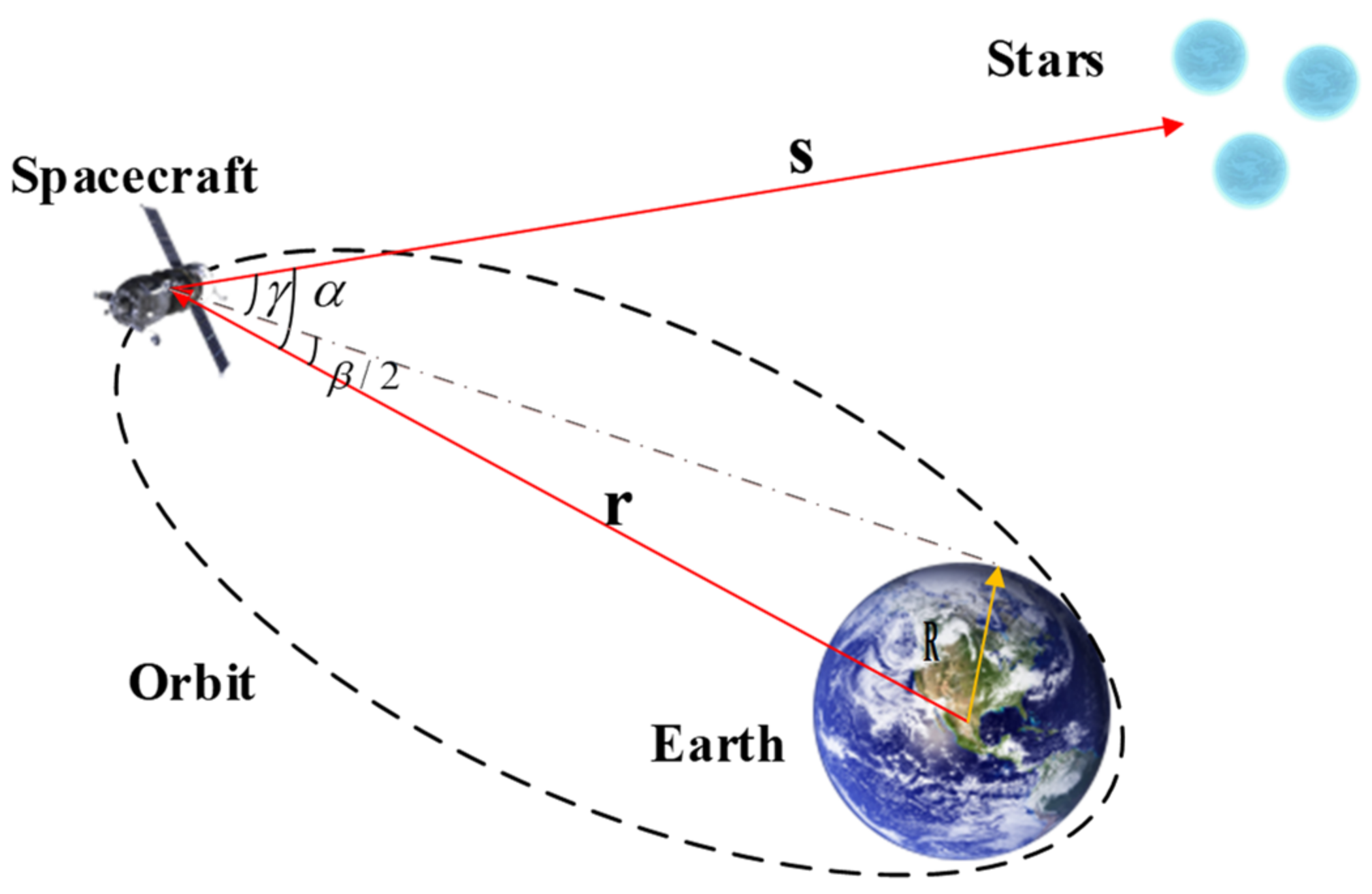
The CNS adopts the measurement model of the direct sensitive horizon and obtains the geocentric vector in the reference coordinate system through the earth sensor. The star sensor is sensitive to stars widely distributed in the celestial sphere to obtain the starlight vector, and the angle between the geocentric vector and the starlight vector of the navigation star is taken as the measurement value. The principle of the celestial navigation measurement model is shown in Figure 1.
Where is the starlight elevation angle, is the Earth’s perspective, is the starlight angle, is the starlight vector, and is the geocentric vector. Obviously, the starlight angle is an analytic function of the position of the spacecraft, and the measurement equation can be established as [11]:
where is the measurement noise.
2.3. BDS Measurement Model
2.3.1. Visibility of BD Satellites
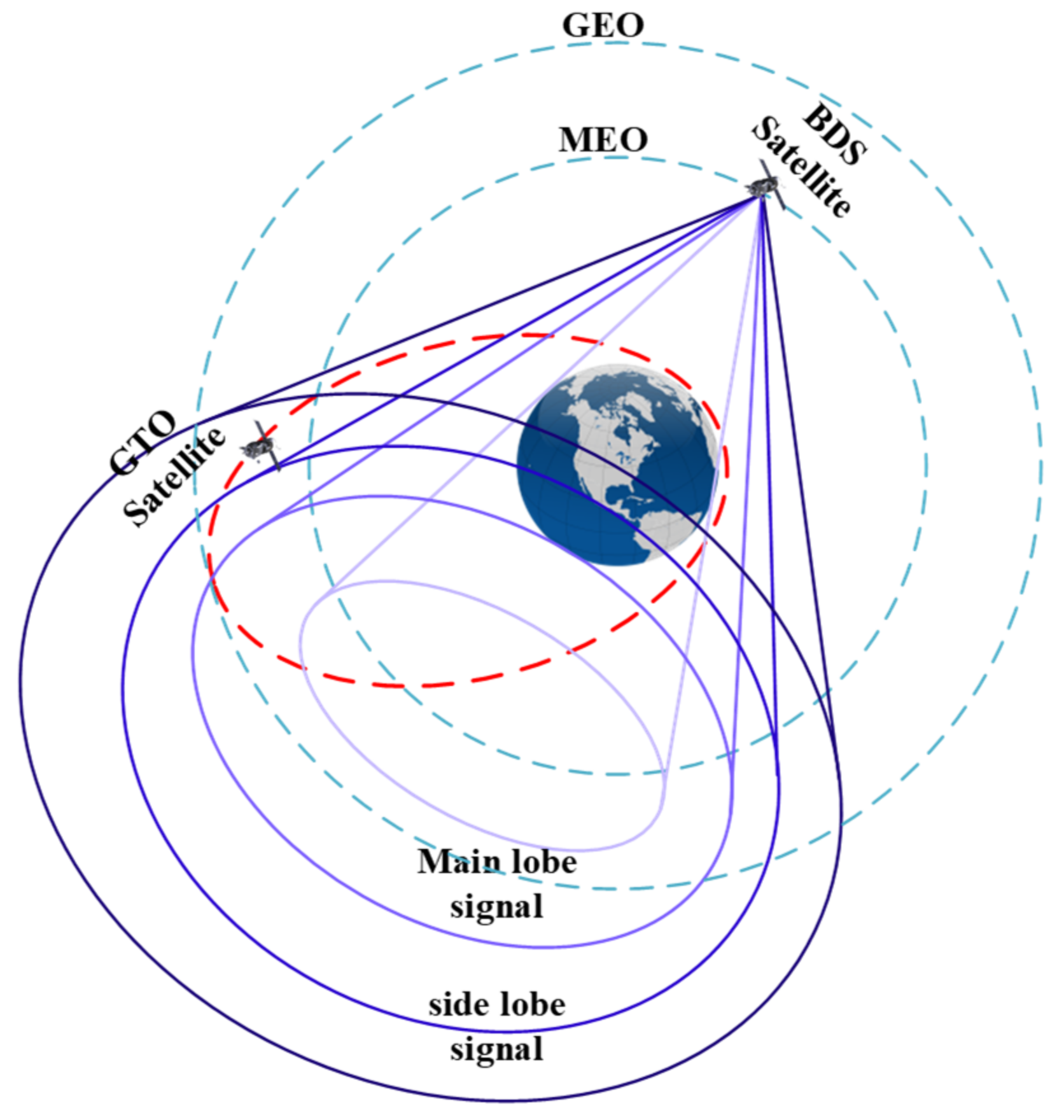
The necessary condition for BDS to be available is that there are enough BD satellites in the BDS constellation to be visible, which is reflected in two aspects. The signal in space is not blocked by the Earth or other celestial bodies, and the geometric relationship is shown in Figure 2. After a series of processes such as amplification and loss, the signal reaches the receiver carried by the GTO satellite; the signal margin can reach the receiver threshold value, and the margin can be calculated by Formula (3) [14].
where is the received signal power; is the signal power; is the transmit antenna gain; is the atmospheric loss; is the path loss; is the sum of other losses, including A/D conversion loss, polarization error loss, etc.; and is the receive antenna gain.
2.3.2. BDS Measurement Equation
Conventional BDS navigation using the pseudorange and pseudorange rates as the measurement values requires four BD satellites’ ephemeris information to solve the coordinates of the carrier and clock bias, which is difficult for GTO satellites to meet in the high-orbit part. In this paper, the relative pseudorange/pseudorange rate is used as the measurement value by the differential method. The effect of clock bias on the navigation system is completely eliminated, i.e.,
where is the GTO satellite state vector; is the reference navigation satellite state vector; is the state of the -th BD satellite except the reference satellite; and are the pseudorange and pseudorange rates from the selected reference navigation satellite to the GTO satellite, respectively; and are the pseudorange and pseudorange rates from the -th navigation satellite to the GTO satellite except the reference navigation satellite, respectively; and and are the measurement noise.
The measurement equation shown in Equation (4) is available when the number of BDS visible satellites is not less than 2. If there are BD satellites visible, a dimensional measurement vector can be constructed. We dynamically adjust the dimension of the measurement vector according to the number of visible BD satellites.
2.4. GTO Satellite CNS/BDS Integrated Navigation Scheme
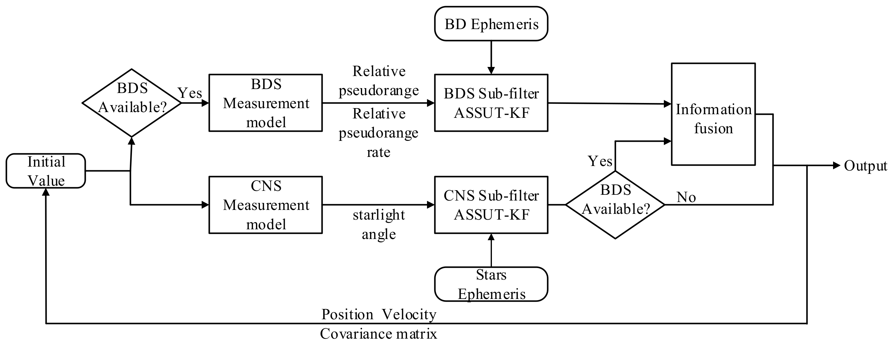
GTO satellite CNS/BDS integrated navigation system: the local optimal estimation of navigation information is obtained through the CNS, and the BDS is used to calculate another local optimal estimation when the BDS is available. Finally, the global optimal estimation is obtained through information fusion. It should be pointed out that when the BDS is not available, we will directly use the CNS estimation for filtering the next cycle. The process of integrated navigation system is shown in Figure 3.
3. GTO Satellite Integrated Navigation ASSUT-FF Algorithm
3.1. Spherical Simplex Unscented Transformation Sampling of ASSUT-FF
Spherical simplex unscented transformation (SSUT) approximates the probability distribution of state variables by selecting sampling points that are randomly distributed on the hypersphere with the state mean as the origin. SSUT replaces the unscented transformation in UKF, which can reduce the computational burden on the on-board computer. The sampling point calculation method is as follows [20,21,22]:
- Step 1: Determine the weight of each sampling point.where is the weight of the first sampling point determined in advance.
- Step 2: Initialization of vector sequence.
- Step 3: Extension of vector sequence.where is the -th sampling point vector of the -dimensional random variable and is the -dimensional zero vector. Therefore, the spherical simplex unscented transformation of an -dimensional random variable with mean and error covariance matrix is
3.2. Adaptive Method of ASSUT-FF
The Kalman filter and its improved algorithm are optimal filters when the prior information of the state space model is accurate and noise is a zero-mean Gaussian distribution, which satisfies the following performance indicators [26]:
The conventional filtering algorithm no longer satisfies Equation (9) when the prior information is inaccurate, and some parameters in the filter need to be corrected in real time so that the innovation sequence is a zero-mean white process, namely, forcing Equation (9) to be established.
3.2.1. Measurement Noise Uncertainty Detection
To avoid the accuracy loss and unnecessary computational burden caused by the adaptive algorithm when the noise prior information is accurate, a method to detect uncertain measurement noise is proposed. Define a statistic using the following:
and follow distribution with a degree of freedom parameter of 1. Where is the detection statistic of the -th dimension measurement value at time , and is the -th element on the diagonal of the matrix. For the selected significance level , through the following:
the enabling threshold of the adaptive factor at this confidence level can be calculated.
3.2.2. Calculation of Adaptive Factor
Define two error vectors as
The time-varying diagonal matrix is introduced to describe the higher-order term error of the above formula; then,
In the same way, define the innovation vector as , and after introducing the time-varying diagonal matrix , then
where and are the state transition matrix and measurement matrix, respectively, which can be derived as follows [27]:
According to the orthogonal law, needs to be established, where is the calculated innovation vector covariance, which can be calculated by [28]
where is the forgetting factor.
can be obtained from ; only an adaptive factor can be introduced such that
Considering the model with a multidimensional measurement vector, each element has different orders of magnitude and physical meanings, and the reliability of the prior information of each element is distinct; the calculation method of the design adaptive factor is as follows:
where , , is the -th element on the diagonal of the matrix.
3.3. Information Fusion Process of ASSUT-FF
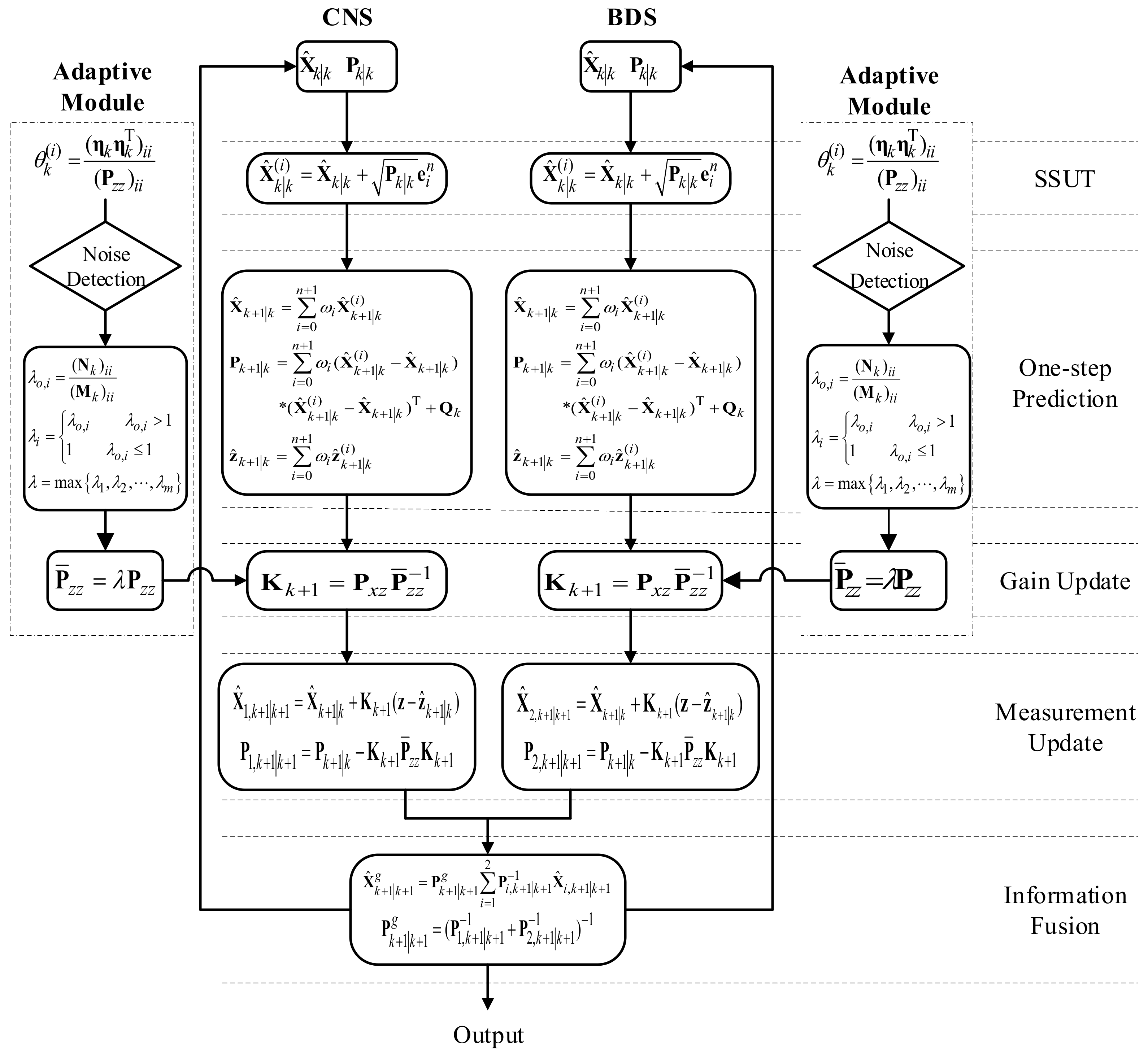
The ASSUT-FF algorithm is divided into the adaptive spherical simplex unscented transformation Kalman filter (ASSUT-KF) and information fusion based on the federated filter. When BDS is available, the celestial navigation ASSUT-KF subfilter and the Beidou navigation ASSUT-KF subfilter run in parallel to obtain the local optimal estimate, and the global optimal estimate is obtained after information fusion. Information fusion is mainly divided into two steps [27].
- Step 1: Distribution of public information.
- Step 2: Local information is fused.where is the information distribution coefficient between 0 and 1 that satisfies .
The flow of the GTO satellite CNS/BDS integrated navigation ASSUT-FF algorithm is shown in Figure 4.
4. Simulation
4.1. BDS Availability Analysis
The geometric positioning method is available when at least four BD satellites are visible, and the CNS/BDS integrated navigation system designed in this paper is available in only two. The variables that affect the availability of BDS mainly consider two aspects of signal properties and receiver sensitivity. The simulation settings [12] are shown in Table 1.
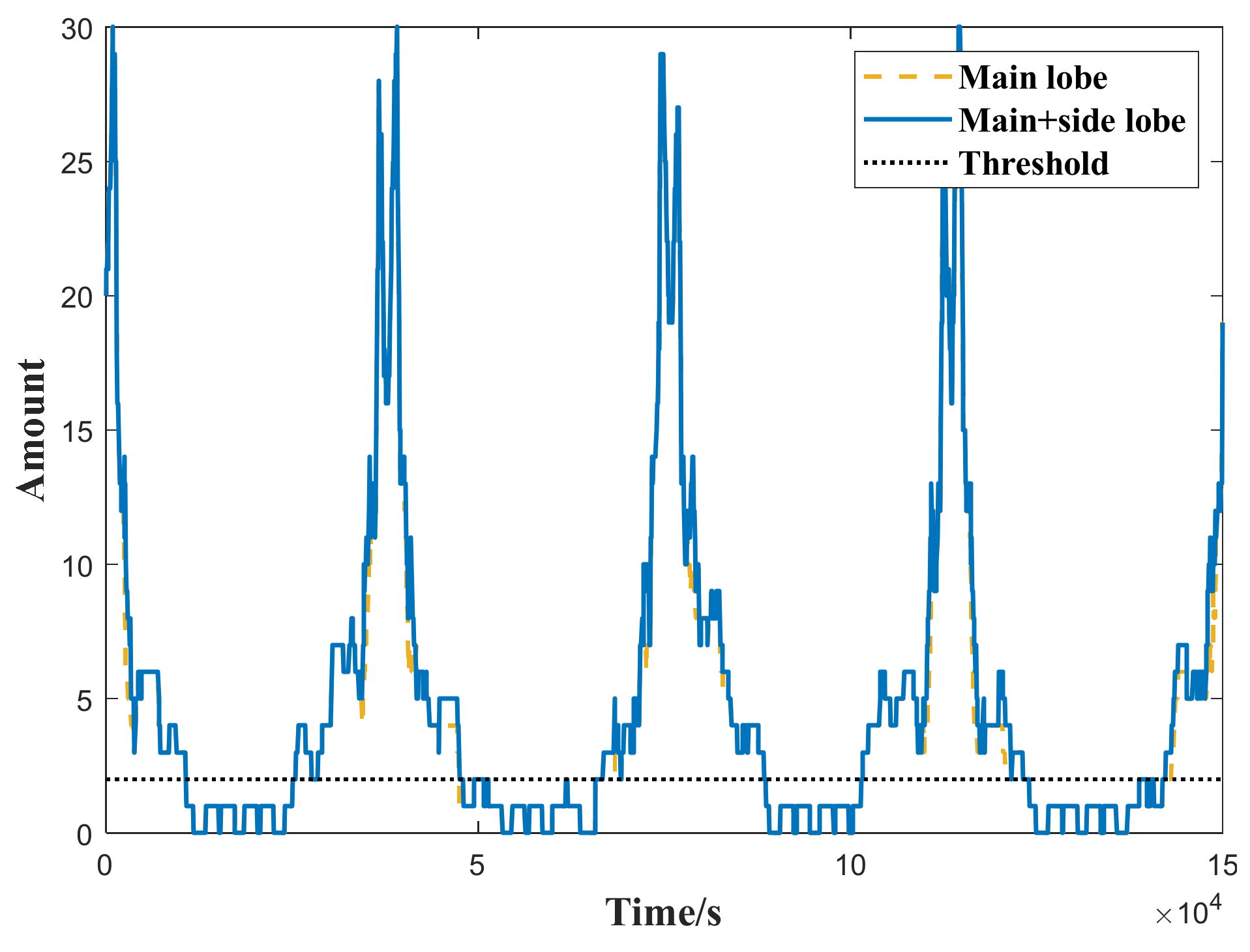
BDS is available to GTO satellites when the number of visible BD satellites is equal to or higher than . is the threshold of the CNS/BDS integrated navigation method, and corresponds to conventional Beidou geometric positioning.
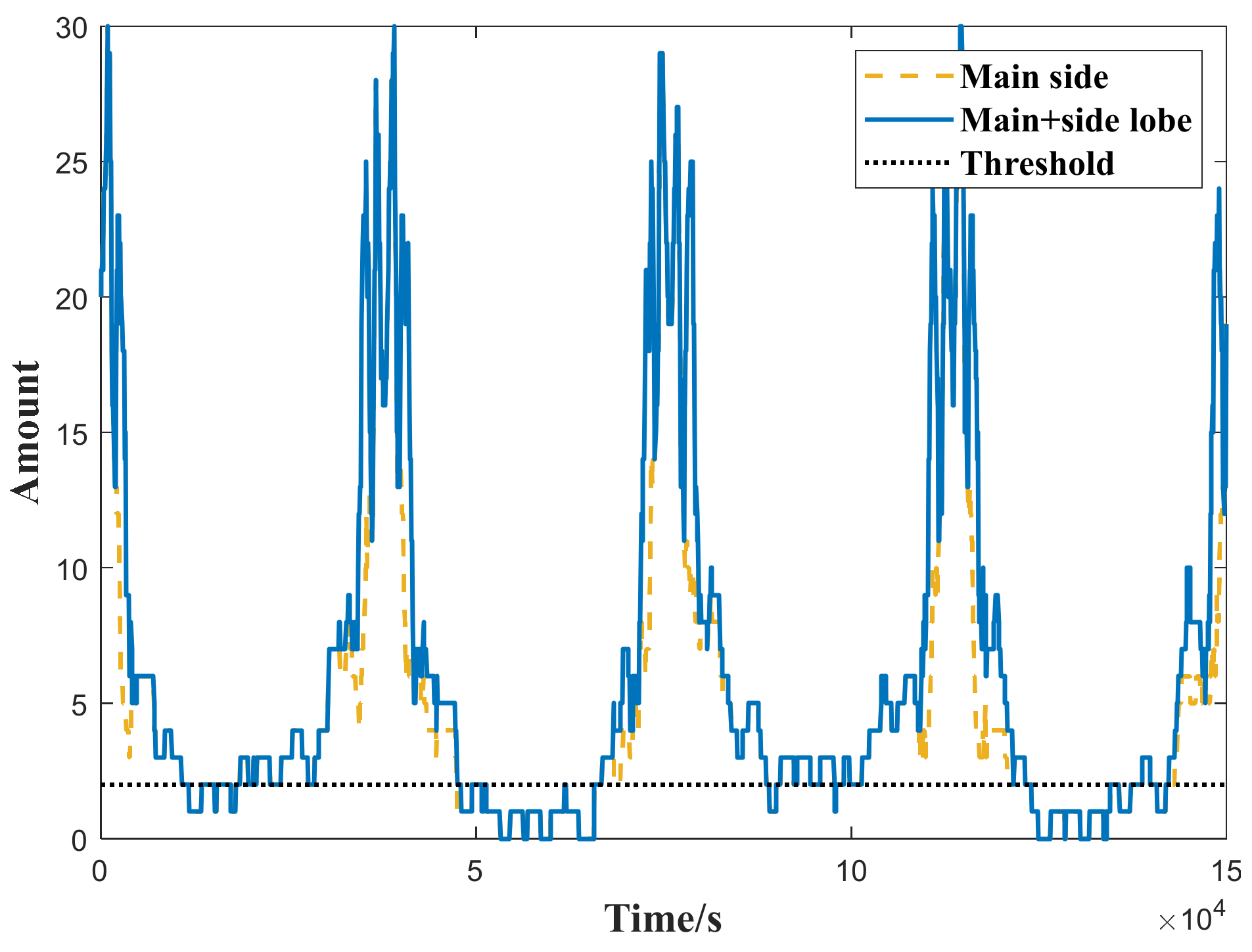
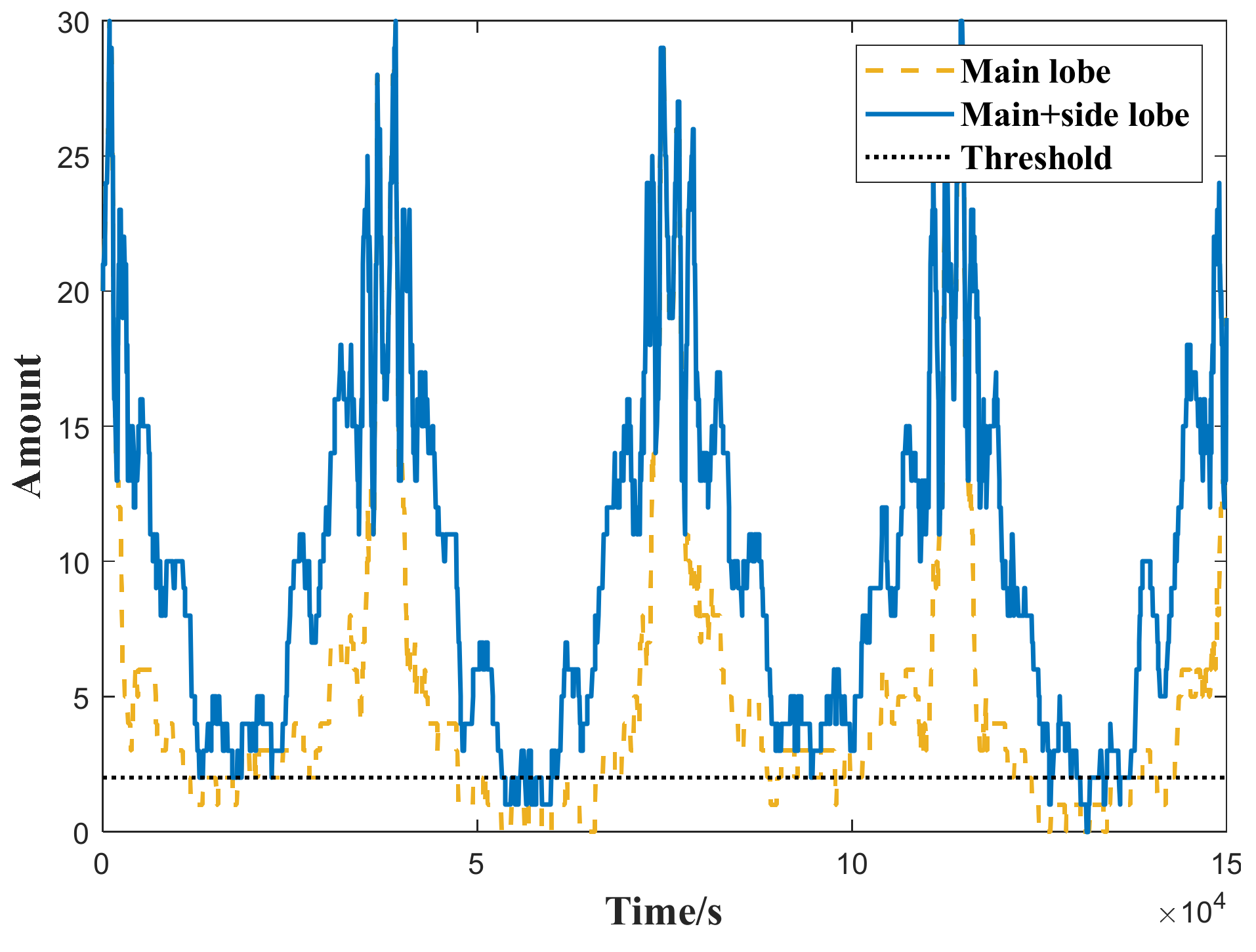
Table 2 and Figure 5, Figure 6 and Figure 7 show that the conventional geometric positioning method and the method proposed in this paper have BDS available time probabilities of 46.47%/49.70%/82.75% and 66.58%/82.29%/96.55%, respectively, corresponding to receiver sensitivity of −170/−175/−180 dBW.
4.2. Comparison of GTO Satellite CNS/BDS Integrated Navigation and CNS Navigation
The CNS/BDS integrated navigation is based on the celestial navigation using the star sensor/earth sensor measurement model. The Beidou measurement model is introduced when BDS is available, and navigation information is calculated by the ASSUT-FF algorithm. The sensors and filter parameter settings are shown in Table 3.
Assuming that all noises constitute zero-mean Gaussian white noise, the basic conditions of the simulation are as follows: GTO semimajor axis 24,478.137 km; eccentricity 0.73126; orbit inclination 28.5°; ascending node right ascension −180°; perigee angular distance 0°; real orbit generated in STK; simulation time T = 150,000 s; and sampling period t = 3 s.
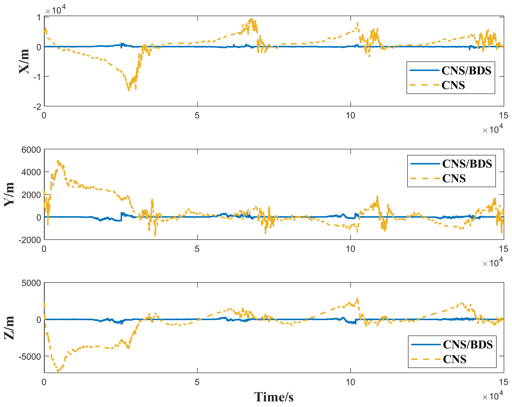
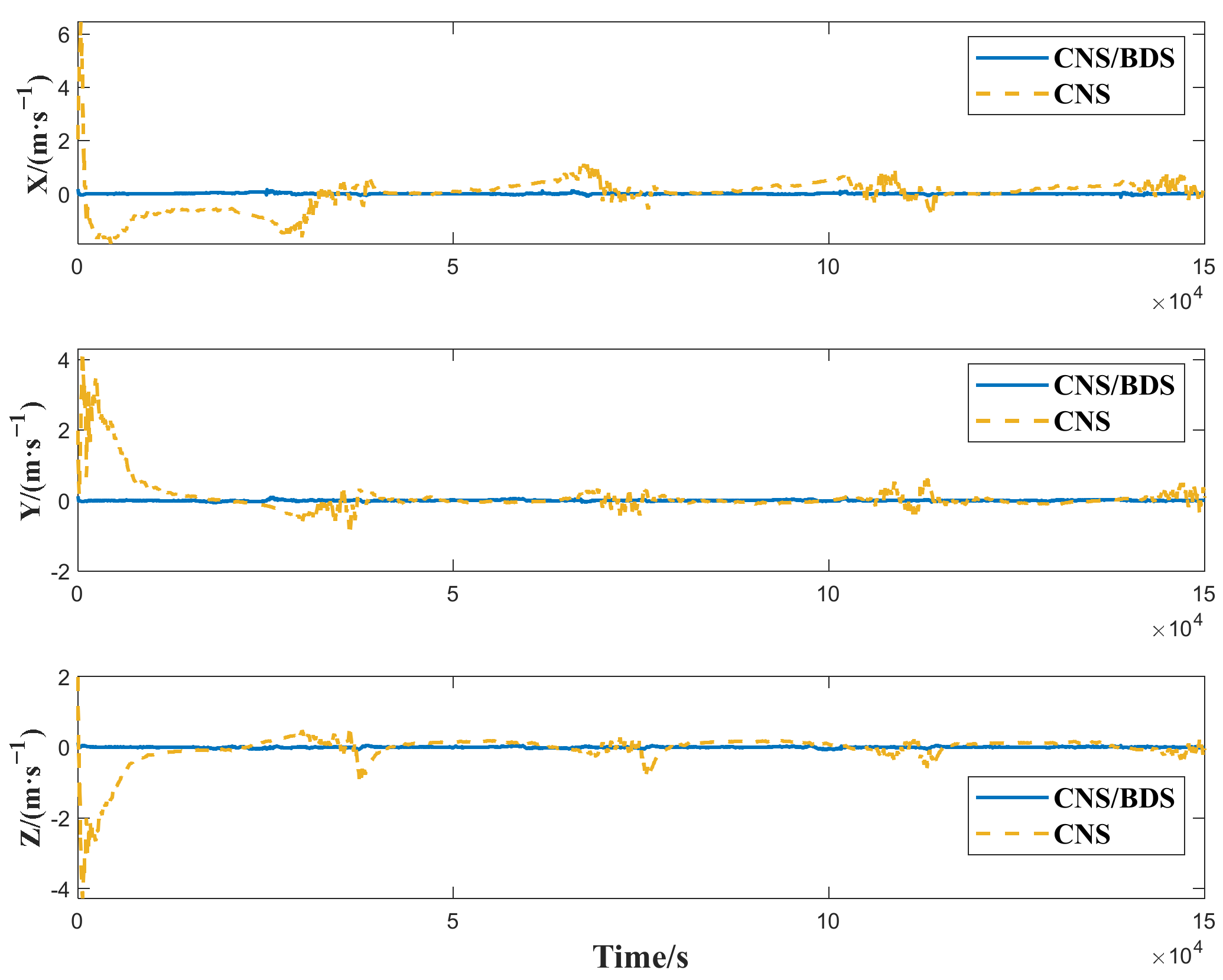
Figure 8 and Figure 9 show the position and velocity errors in three directions of the two methods, and Table 4 shows the root mean square error (RMSE). The orbit determination error in the three directions of CNS navigation is more than 1000 m, while the orbit determination errors in the three directions of CNS/BDS integrated navigation are less than 200 m. When BDS is available, Beidou navigation information can correct the periodic error existing in single celestial navigation. Certain error fluctuations will only occur briefly when BDS is not available. Compared with CNS navigation, the CNS/BDS integrated navigation improves the accuracy by approximately 96.23%.
4.3. Comparison of GTO Satellite CNS/BDS Integrated Navigation and BDSGPA-CNS Navigation
The conventional Beidou Navigation System Geometric Positioning Assisted Celestial Navigation System (BDSGPA-CNS) calculates the accurate position and velocity of spacecraft through geometric methods when BDS is available to correct the estimated values of the celestial navigation system. The availability of BDS when GTO satellites use conventional BDSGPA-CNS navigation and the CNS/BDS integrated navigation proposed in this paper have been analyzed in Section 3.1. This section compares the navigation effects of the two methods. The sensors and filter parameter settings are shown in Table 5.
Assuming that all the noises constitute zero-mean Gaussian white noise, the basic conditions of the simulation are as follows: GTO semimajor axis 24,478.137 km; eccentricity 0.73126; orbit inclination 28.5°; ascending node right ascension −180°; perigee angular distance 0°; real orbit generated in STK; simulation time T = 150,000 s; and sampling period t = 3 s.
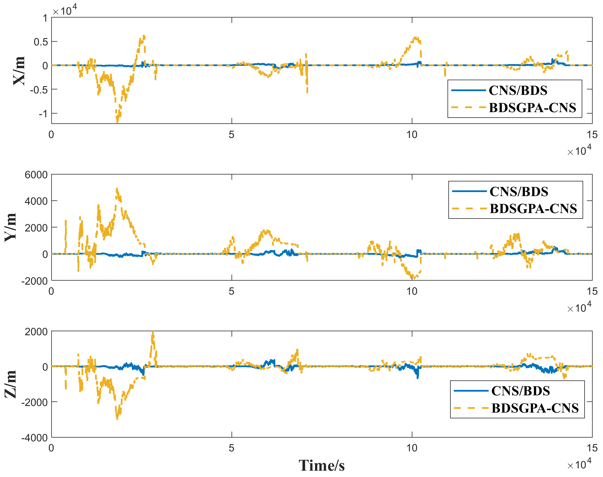
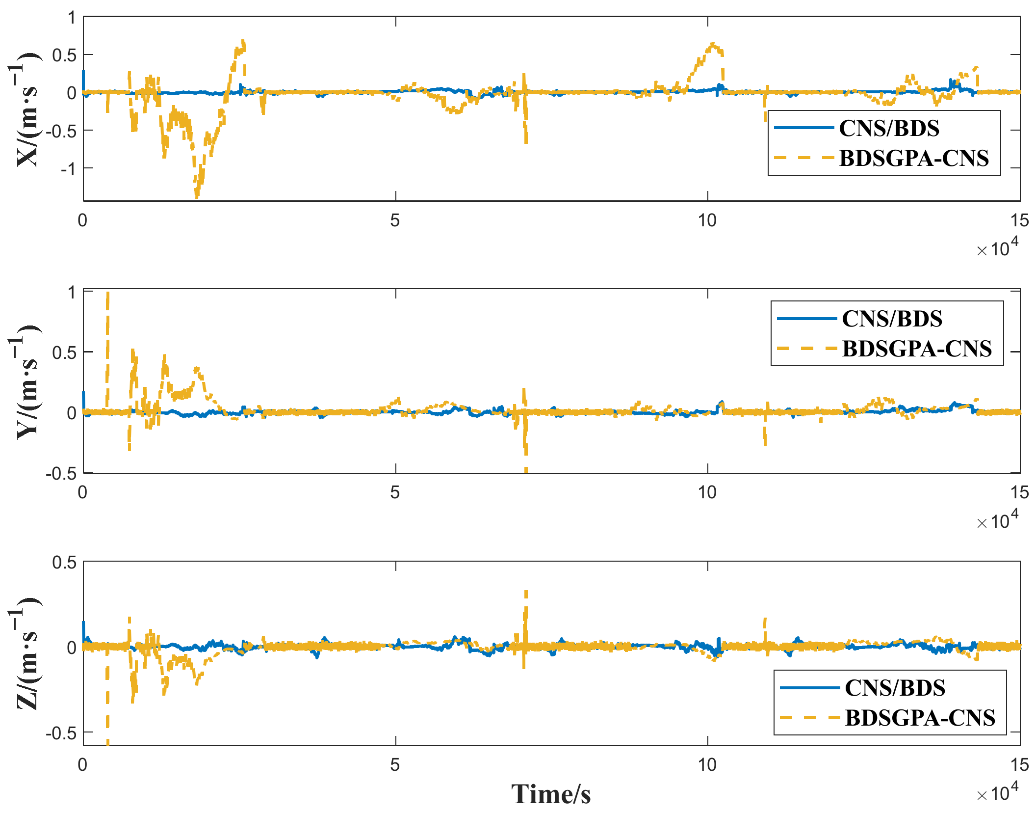
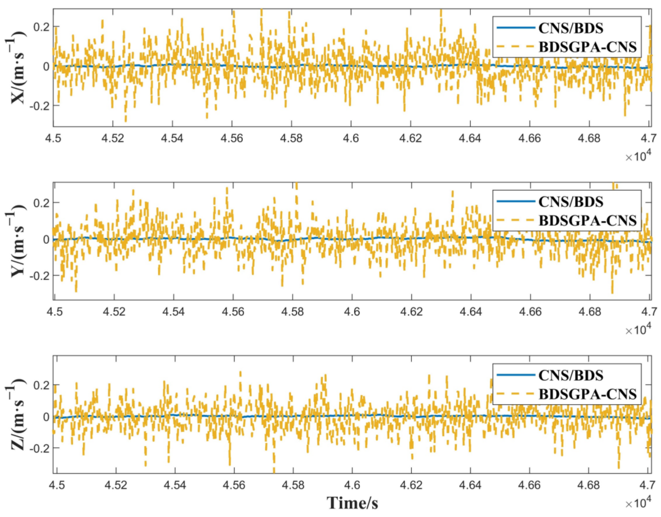
Figure 10 and Figure 11 show the position and velocity errors in three directions of the two methods, and Table 6 shows the RMSEs. Among them, the orbit determination errors in the three directions of BDSGPA-CNS are 1258.2 m, 758.2 m and 339.8 m, and the orbit determination errors in the three directions of BDS/CNS are 170.7 m, 87.9 m and 78.2 m. There is a large error in CNS navigation alone when BDSGPA-CNS navigation does not meet the requirement of at least four BD satellites being visible, while CNS/BDS integrated navigation improves the availability of BDS, shortens the CNS navigation section with large errors, and improves the navigation accuracy by approximately 84.06%.
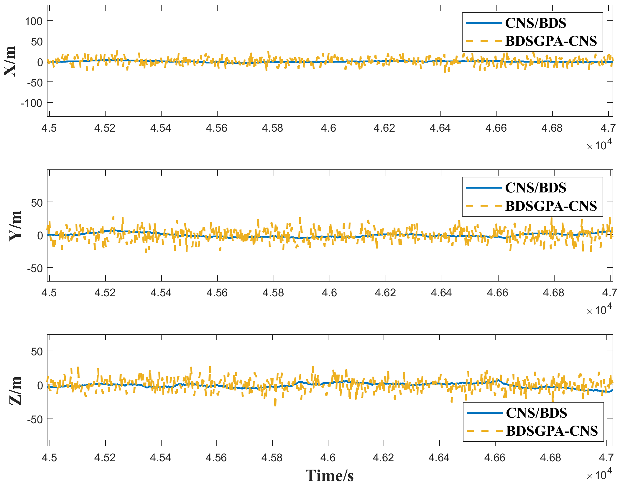
When there are no fewer than four visible BD satellites, the local error curve comparing the BDSGPA-CNS method and the CNS/BDS integrated navigation method is shown in Figure 12 and Figure 13 and Table 7. The orbit determination error of the BDSGPA-CNS method is approximately tens of meters, while it is only a few meters for the CNS/BDS integrated navigation, and it still has better performance when both methods are available.
4.4. Case Where Prior Information Is Inaccurate
The sensors and filter parameter settings are shown in Table 8.
Affected by the spatial environment, the measurement noise cannot be only zero-mean Gaussian white noise with constant amplitude. Assuming that within the simulation time of 87,000–96,000 s, the CNS measurement noise becomes
Within 72,000–81,000 s, the BDS measurement noise becomes
where and are the prior statistics of the noise covariance of the CNS measurement model and BDS measurement model, respectively.
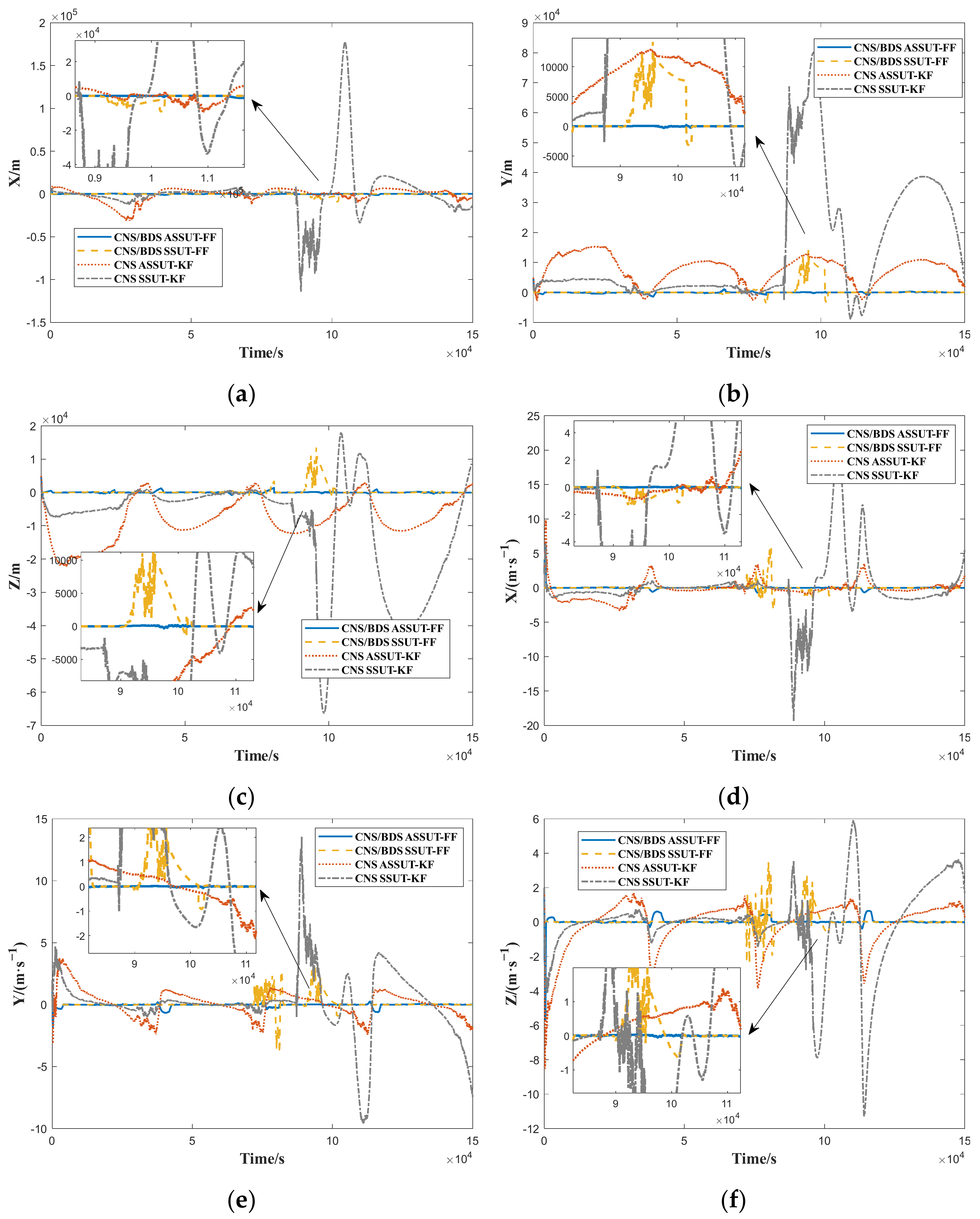
Figure 14 shows the position and velocity errors in three directions, and Table 9 and Table 10 show the RMSEs when we use the spherical simplex unscented transformation Kalman filter (SSUT-KF)/adaptive spherical simplex unscented transformation Kalman filter (ASSUT-KF) algorithm CNS navigation and spherical simplex unscented transformation federated Kalman filter (SSUT-FF)/adaptive spherical simplex unscented transformation federated Kalman filter (ASSUT-FF) algorithm CNS/BDS integrated navigation. The adaptive algorithm proposed in this paper has better robustness when the performance of the GTO satellite onboard sensors is degraded by a complex environment.
4.5. Case of Different Noise Levels
The simulation of GTO satellite CNS/BDS integrated navigation under different noise levels is carried out, and the navigation accuracy of the ASSUT-FF and SSUT-FF algorithms in uncertain noise areas is compared.
The sensors and filter parameters settings are shown in Table 11.
The basic simulation conditions are as follows: GTO semimajor axis 24,478.137 km; eccentricity 0.73126; orbit inclination 28.5°; ascending node right ascension −180°; perigee angular distance 0°; real orbit generated in STK; simulation time T = 150,000 s; and sampling period t = 3 s. Uncertain noise is still considered as white noise with an amplitude increase of and a constant noise of , and the definition level coefficient is . The CNS measurement model constant noise is , and corresponds to the BDS measurement model:
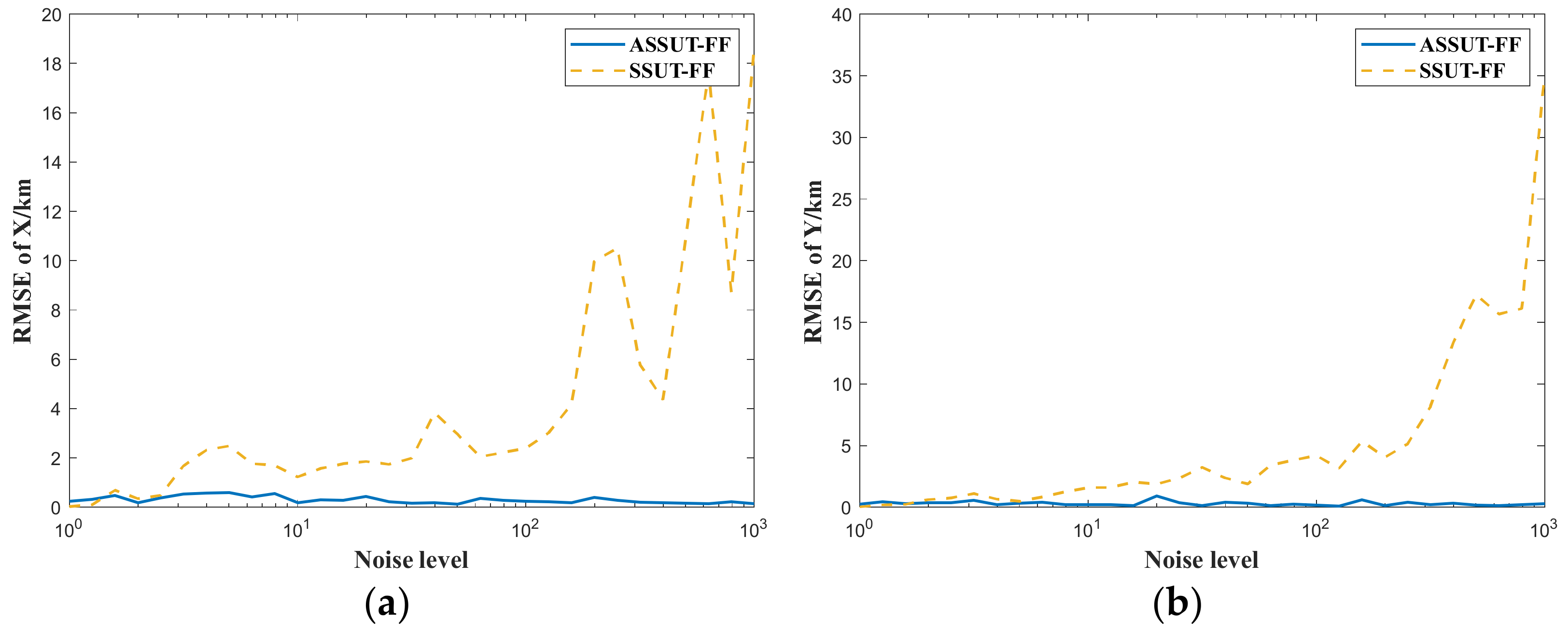
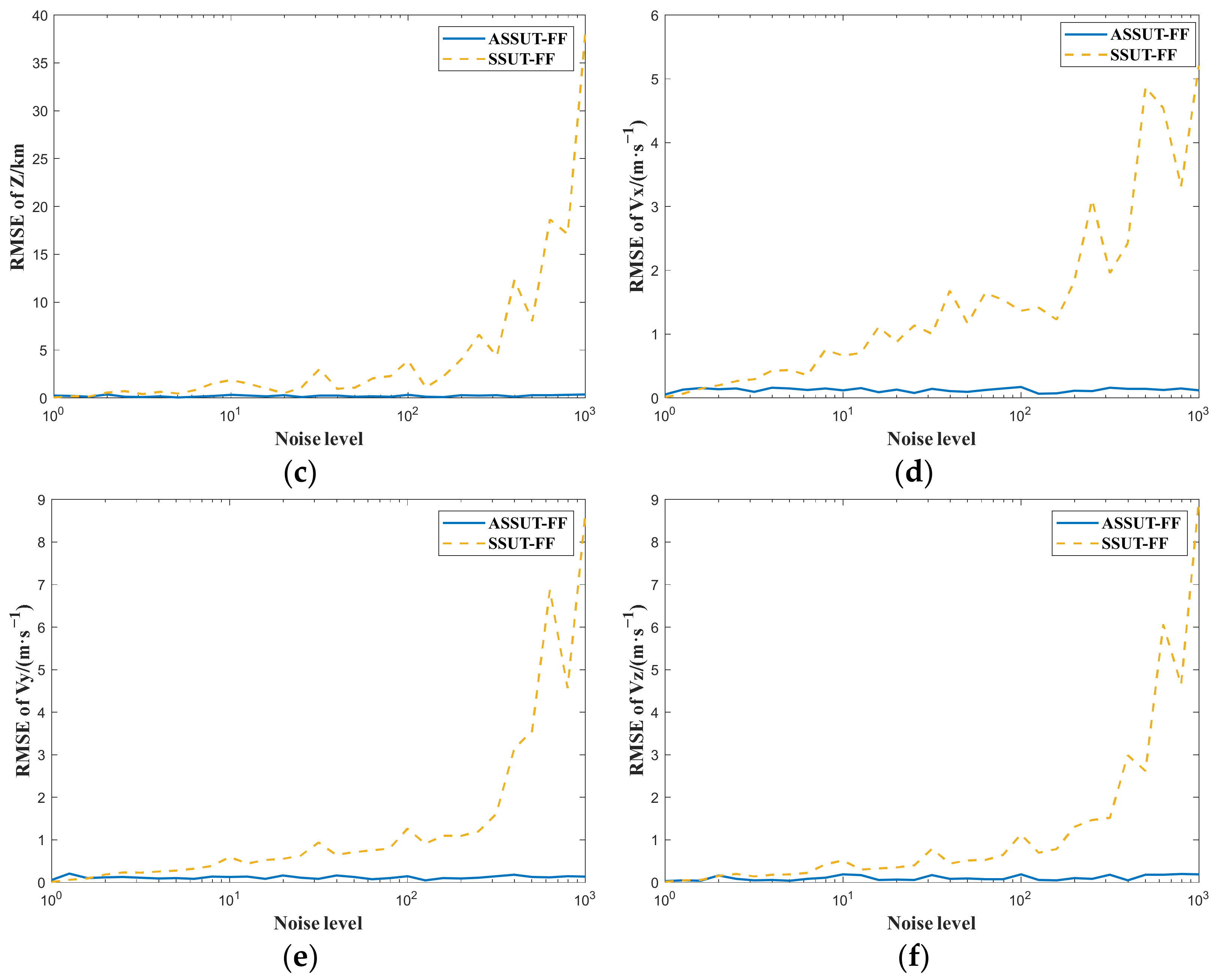
Figure 15 shows the RMSEs of position and velocity in three directions at different noise levels of CNS/BDS integrated navigation using the SSUT-FF algorithm and ASSUT-FF algorithm, respectively, in the uncertain noise area. Table 12 shows the average RMSEs. The mean orbit determination errors in the three directions using the SSUT-FF algorithm are 4159.2 m, 5094.4 m, and 4431.6 m, while 298.2 m, 299.8 m, and 210.3 m correspond to the ASSUT-FF algorithm. The ASSUT-FF algorithm can still maintain ideal working performance when the complex space environment causes the accuracy of the sensors to decrease.
5. Conclusions
This paper establishes a BDS measurement model based on a dynamic dimensional measurement vector based on the relative pseudorange/pseudorange rate, which eliminates the effect of clock bias and expands the time available for BDS. Considering that the complex space environment of the GTO satellite may degrade the performance of onboard sensors, this paper proposes an ASSUT-FF algorithm based on the strong tracking concept. The simulation results show that the designed CNS/BDS integrated navigation system improves the available time of BDS. Compared with CNS navigation and BDSGPA-CNS navigation, the orbit determination error of CNS/BDS integrated navigation is increased by 96.23% and 84.06%, respectively. In addition, the CNS/BDS integrated navigation based on the ASSUT-FF algorithm still has good performance when the space environment is complex.
The GTO satellite CNS/BDS integrated navigation ASSUT-FF algorithm designed in this paper solves the periodic error fluctuation problem of GTO satellite celestial navigation and can realize high-precision autonomous navigation of GTO satellites, which can also be used for high-precision autonomous navigation of a series of HEO satellites such as “Molniya” and “Meridian”.
Author Contributions
B.H. provided the overall research ideas for the thesis and put forward constructive suggestions for the writing of the thesis; X.W. participated in the discussion of the research ideas of the thesis and completed the simulation experiments and manuscript writing; and Y.W. and Z.C. provided instructions for the research and thesis writing. All authors have read and agreed to the published version of the manuscript.
Funding
This research was funded by National Natural Science Foundation of China (Nos. 61973153; Nos. 62073165).
Institutional Review Board Statement
Not applicable.
Informed Consent Statement
Not applicable.
Data Availability Statement
The data presented in this study are available on request from the corresponding author.
Conflicts of Interest
The authors declare no conflict of interest.
References
- Li, X.; Zhang, R.; Han, C. Low-thrust GEO orbit transfer guidance using semi-analytic method. Adv. Astronaut. Sci. 2018, 162, 2881–2892. [Google Scholar]
- Li, J.; Li, H.; Li, B.; Zhang, Y.; Zeng, Q. Satellite celestial/cadar altimeter integrated navigation method for large elliptical orbits. Chin. J. Inert. Technol. 2012, 20, 300–305. [Google Scholar]
- Wu, W.; Ning, X.; Liu, L. New celestial assisted INS initial alignment method for lunar explorer. J. Syst. Eng. Electron. 2013, 24, 108–117. [Google Scholar] [CrossRef]
- Xin, M.; Ning, X.; Fang, J. Analysis of orbital dynamic equation in navigation for a mars gravity-assist mission. J. Navig. 2012, 65, 531–548. [Google Scholar]
- Guan, M.; Xu, T.; Li, M.; Gao, F.; Ma, D. Navigation in GEO, HEO, and Lunar Trajectory Using Multi-GNSS Sidelobe Signals. Remote Sens. 2022, 2, 318. [Google Scholar] [CrossRef]
- Li, Q. GNSS-based orbit determination for highly elliptical orbit satellites. In Proceedings of the International Global Navigation Satellite Systems Society IGNSS Symposium, New York, NY, USA, 1 January 2012. [Google Scholar]
- Wang, C.; Liu, R.; Li, B. Application of unscented kalman filter in celestial/geomagnetic autonomous navigation algorithm of aerocraft. J. Chin. Inert. Technol. 2010, 18, 543–549. [Google Scholar]
- Quan, W.; Fang, J.; Xu, F.; Sheng, W. Hybrid simulation system study of SINS/CNS integrated navigation. IEEE Aerosp. Electron. Syst. Mag. 2008, 23, 17–24. [Google Scholar] [CrossRef]
- Gao, S.; Zhong, Y.; Zhang, X.; Shirinzadeh, B. Multi-sensor optimal data fusion for INS/GPS/SAR integrated navigation system. Aerosp. Sci. Technol. 2009, 13, 232–237. [Google Scholar] [CrossRef] [Green Version]
- Ji, X.; Gao, L.; Liu, Z.; Hua, Z. Spacecraft autonomous navigation system based on SINS/Ultraviolet sensor/Star sensor. In Proceedings of the IEEE Chinese Guidance, Navigation and Control Conference (CGNCC), Nanjing, China, 12–14 August 2016. [Google Scholar]
- Wang, P.; Zhang, Y. A new method for autonomous navigation of HEO satellite based on celestial/accelerometer. Chin. J. Inert. Technol. 2014, 22, 525–530. [Google Scholar]
- Huo, M. Research on Autonomous Navigation Technology of High-Orbit Satellites Based on Celestial/GNSS. Ph.D. Thesis, National University of Defense Technology, Changsha, China, 2016. [Google Scholar]
- Li, J.; Zhang, Y.; Zheng, J.; Gao, D. Integrated navigation method for large elliptical orbit satellite based on information fusion. J. Astronaut. 2012, 33, 1233–1240. [Google Scholar]
- Wang, P.; Zhang, Y. Celestial navigation method of HEO satellite based on celestial/GPS. Control Decis. 2015, 30, 519–525. [Google Scholar]
- Chen, J.; Josep, J.; Gerard, G.; Yuan, J. An efficient statistical adaptive order-switching methodology for kalman filters. Commun. Nonlinear Sci. Numer. Simul. 2021, 93, 105539. [Google Scholar] [CrossRef]
- Huang, Y.; Zhang, Y.; Xu, B.; Wu, Z.; Chambers, J. A New Adaptive Extended Kalman Filter for Cooperative Localization. IEEE Trans. Aerosp. Electron. Syst. 2018, 54, 353–368. [Google Scholar] [CrossRef]
- Zarei, J.; Abdolrahman, R. Performance improvement for mobilerobot position determination using cubature kalman filter. J. Navig. 2018, 71, 389–402. [Google Scholar] [CrossRef]
- Bonya, K.; Ghorbani, S.; Janabi, S. Unscented kalman filter state estination for manipulating unmanned aerial vehicles. Aerosp. Sci. Technol. 2019, 92, 446–463. [Google Scholar]
- Tang, C.; Hu, X.; Zhou, S.; Guo, R.; He, F.; Liu, L.; Zhu, L.; Li, X.; Wu, S.; Zhao, G.; et al. Improvement of orbit determination accuracy for beidou navigation satellite system with two-way satellite time frequency transfer. Adv. Space Resharch 2016, 58, 1390–1400. [Google Scholar] [CrossRef]
- Jia, K.; Pei, Y.; Gao, Z.; Zhong, Y.; Gao, S.; Wei, W.; Hu, G. A Quaternion-Based Robust Adaptive Spherical Simplex Unscented Particle Filter for MINS/VNS/GNS Integrated Navigation System. Math. Probl. Eng. 2019, 2019, 8532601. [Google Scholar] [CrossRef] [Green Version]
- Zhao, F.; Ge, S.; Zhang, J.; He, W. Celestial navigation in deep space exploration using spherical simplex unscented particle filter. IET Signal Process 2017, 12, 463–470. [Google Scholar] [CrossRef]
- Peng, S.; Pang, X.; Chen, H.; Lin, Y.; Zuo, Z.; Yu, H.; Tang, J. Comparison on three unscented transformation methods for solving probabilistic load flow. In Proceedings of the IEEE Innovative Smart Grid Technologies—Asia (ISGT Asia), Chengdu, China, 21–24 May 2019. [Google Scholar]
- Huang, Y.; Zhang, Y.; Xu, Z.; Li, N.; Chambers, J. A novel adaptive kalman filter with inaccurate process and measurement noise covariance matrices. IEEE Trans. Autom. Control 2018, 63, 594–601. [Google Scholar] [CrossRef] [Green Version]
- Kwang, H.; Jang, G.; Chan, G.; Gyu, I. The stability analysis of the adaptive fading extended kalman filter. In Proceedings of the 16th IEEE International Conference on Control Applications, Singapore, 1–3 October 2007. [Google Scholar]
- Zhang, W. Satellite Orbit Attitude Dynamics and Control; Beijing University of Aeronautics and Astronautics Press: Beijing, China, 1998; pp. 49–51. ISBN 978-78-1012-721-9. [Google Scholar]
- Qing, Y.; Zhang, H.; Wang, S. Kalman Filter and Principle of Integrated Navigation; Northwestern Polytechnic University Press: Xi’an, China, 2010; pp. 86–107. ISBN 978-75-6123-350-4. [Google Scholar]
- Cao, Y.; Tian, X. An adaptive UKF algorithm for process fault prognostics. In Proceedings of the 2th International Conferences on Intelligent Computation Technology and Automation, Changsha, China, 10–11 October 2009. [Google Scholar]
- Zhang, H.; Xie, J.; Ge, J.; Zong, B.; Lu, W. Strong tracking square root volumetric kalman filtering algorithm for adaptive CS model. J. Syst. Eng. Electron. 2019, 41, 1186–1194. [Google Scholar]
Figure 1.
Principle of celestial navigation measurement.

Figure 2.
Geometric relationship between the BDS constellation and GTO.

Figure 3.
CNS/BDS integrated navigation scheme.

Figure 4.
ASSUT-FF algorithm procedure.

Figure 5.
Visibility of GTO satellites to BD satellites when the receiver sensitivity is −170 dBW.

Figure 6.
Visibility of GTO satellites to BD satellites when the receiver sensitivity is −175 dBW.

Figure 7.
Visibility of GTO satellites to BD satellites when the receiver sensitivity is −180 dBW.

Figure 8.
Position error in three directions.

Figure 9.
Velocity error in three directions.

Figure 10.
Position error in three directions.

Figure 11.
Velocity error in three directions.

Figure 12.
Local position error in three directions.

Figure 13.
Local velocity error in three directions.

Figure 14.
Position and velocity errors in three directions. (a) Position error in the X direction; (b) position error in the Y direction; (c) position error in the Z direction; (d) velocity error in the X direction; (e) velocity error in the Y direction; and (f) velocity error in the Z direction.
Figure 14.
Position and velocity errors in three directions. (a) Position error in the X direction; (b) position error in the Y direction; (c) position error in the Z direction; (d) velocity error in the X direction; (e) velocity error in the Y direction; and (f) velocity error in the Z direction.

Figure 15.
RMSEs of position and velocity in three directions at different noise levels. (a) RMSEs of the position in the X direction; (b) RMSEs of the position in the Y direction; (c) RMSEs of the position in the Z direction; (d) RMSEs of velocity in the X direction; (e) RMSEs of velocity in the Y direction; and (f) RMSEs of velocity in the Z direction.


Table 1.
BDS simulation parameters.
| Frequency /GHz | Main Lobe Angle/° | Power /dBW | Main Lobe Gain/dB | Side Lobe Gain/dB | Receiver Sensitivity /dBW | Other Losses /dB |
|---|---|---|---|---|---|---|
| 1.5611 | 42.6 | 12 | 15 | 3 | −170/−175/−180 | 3 |
Table 2.
Probability of visibility of GTO satellite to BDS in one cycle.
| N | Signal Properties | Probability of Availability of BDS for Receivers of Different Sensitivities | ||
|---|---|---|---|---|
| −170 dBW | −175 dBW | −180 dBW | ||
| 2 | Main + side lobe signal | 66.58% | 82.29% | 96.55% |
| Main lobe signal | 66.58% | 82.29% | 82.29% | |
| 4 | Main + side lobe signal | 46.47% | 49.70% | 82.75% |
| Main lobe signal | 45.67% | 47.07% | 47.07% | |
Table 3.
Sensors and filters parameter settings.
| Star Sensor | Earth Sensor | Receiver | Pseudorange Error | Pseudorange Rate Error | CNS Noise Variance | BDS Noise Variance | Initial Error |
|---|---|---|---|---|---|---|---|
| −170 dBW | 10 m | 0.1 m/s |
Table 4.
RMSEs of the position and velocity of the CNS and CNS/BDS in three directions.
| x/m | y/m | z/m | vx/(m/s) | vy/(m/s) | vz/(m/s) | Increased Accuracy | |
|---|---|---|---|---|---|---|---|
| CNS | 3607.1 | 1277.7 | 2021.8 | 0.6229 | 0.5025 | 0.4590 | -- |
| CNS/BDS | 132.9 | 83.1 | 96.8 | 0.0203 | 0.0153 | 0.0162 | 96.23% |
Table 5.
Sensors and filter parameter settings.
| Star Sensor | Earth Sensor | Receiver | Pseudorange Error | Pseudorange Rate Error | CNS Noise Variance | BDS Noise Variance | Initial Error |
|---|---|---|---|---|---|---|---|
| −170 dBW | 10 m | 0.1 m/s |
Table 6.
Comparison of CNS/BDS integrated navigation and BDSGPA-CNS navigation errors.
| x/m | y/m | z/m | vx/(m/s) | vy/(m/s) | vz/(m/s) | Increased Accuracy | |
|---|---|---|---|---|---|---|---|
| BDSGPA-CNS | 1258.2 | 758.2 | 339.8 | 0.1539 | 0.0657 | 0.0367 | -- |
| CNS/BDS | 170.7 | 87.9 | 78.2 | 0.0237 | 0.0141 | 0.0144 | 84.06% |
Table 7.
RMSEs for position and velocity in each direction when both methods are available.
| x/m | y/m | z/m | vx/(m/s) | vy/(m/s) | vz/(m/s) | |
|---|---|---|---|---|---|---|
| BDSGPA-CNS | 34.5104 | 43.3258 | 13.7668 | 0.0928 | 0.0983 | 0.1096 |
| CNS/BDS | 1.4396 | 2.1284 | 3.0380 | 0.0047 | 0.0058 | 0.0050 |
Table 8.
Sensors and filter parameters settings.
| Star Sensor | Earth Sensor | Receiver | Pseudorange Error | Pseudorange Rate Error | CNS Noise Variance | BDS Noise Variance | Initial Error |
|---|---|---|---|---|---|---|---|
| −170 dBW | 10 m | 0.1 m/s |
Table 9.
RMSEs of position and velocity in three directions for the full simulation time.
| Algorithm | x/m | y/m | z/m | vx/(m/s) | vy/(m/s) | vz/(m/s) | |
|---|---|---|---|---|---|---|---|
| CNS | SSUT-KF | 30,975.5 | 24,338.6 | 18,419.2 | 4.1487 | 2.5703 | 2.3528 |
| ASSUT-KF | 7691.4 | 8984.2 | 10,274.9 | 1.3007 | 1.0766 | 1.3449 | |
| CNS/BDS | SSUT-FF | 1339.1 | 2184.4 | 1550.2 | 0.5539 | 0.5234 | 0.4313 |
| ASSUT-FF | 420.9 | 248.9 | 239.7 | 0.3283 | 0.1497 | 0.2741 |
Table 10.
RMSEs of position and velocity in three directions in the uncertain noise region.
| Algorithm | x/m | y/m | z/m | vx/(m/s) | vy/(m/s) | vz/(m/s) | |
|---|---|---|---|---|---|---|---|
| CNS | SSUT-KF | 38,203.1 | 33,384.5 | 6892.3 | 5.6796 | 3.5540 | 1.1270 |
| ASSUT-KF | 4511.2 | 7477.6 | 9498.8 | 1.0734 | 1.0040 | 1.2253 | |
| CNS/BDS | SSUT-FF | 2046.3 | 3281.3 | 2810.5 | 1.3465 | 1.2411 | 1.0291 |
| ASSUT-FF | 163.1 | 192.6 | 332.1 | 0.1466 | 0.1285 | 0.1876 |
Table 11.
Sensors and filter parameter settings.
| Star Sensor | Earth Sensor | Receiver | Pseudorange Error | Pseudorange Rate Error | CNS Noise Variance | BDS Noise Variance | Initial Error |
|---|---|---|---|---|---|---|---|
| −170 dBW | 10 m | 0.1 m/s |
Table 12.
Average RMSEs of position and velocity in three directions in the uncertain noise region.
| Algorithm | x/m | y/m | z/m | vx/(m/s) | vy/(m/s) | vz/(m/s) |
|---|---|---|---|---|---|---|
| SSUT-FF | 4159.2 | 5094.4 | 4431.6 | 1.4752 | 1.3752 | 1.2467 |
| ASSUT-FF | 298.2 | 299.8 | 210.3 | 0.1244 | 0.1179 | 0.1025 |
Publisher’s Note: MDPI stays neutral with regard to jurisdictional claims in published maps and institutional affiliations. |
© 2022 by the authors. Licensee MDPI, Basel, Switzerland. This article is an open access article distributed under the terms and conditions of the Creative Commons Attribution (CC BY) license (https://creativecommons.org/licenses/by/4.0/).
Share and Cite
MDPI and ACS Style
Hua, B.; Wei, X.; Wu, Y.; Chen, Z. Design of the ASSUT-FF Algorithm for GTO Satellite CNS/BDS Integrated Navigation. Aerospace 2022, 9, 384. https://doi.org/10.3390/aerospace9070384
AMA Style
Hua B, Wei X, Wu Y, Chen Z. Design of the ASSUT-FF Algorithm for GTO Satellite CNS/BDS Integrated Navigation. Aerospace. 2022; 9(7):384. https://doi.org/10.3390/aerospace9070384
Chicago/Turabian StyleHua, Bing, Xiaosong Wei, Yunhua Wu, and Zhiming Chen. 2022. "Design of the ASSUT-FF Algorithm for GTO Satellite CNS/BDS Integrated Navigation" Aerospace 9, no. 7: 384. https://doi.org/10.3390/aerospace9070384
Note that from the first issue of 2016, this journal uses article numbers instead of page numbers. See further details here.