A Modified RANS Model for Drag Prediction of Practical Configuration with Riblets and Experimental Validation

1
School of Astronautics, Northwestern Polytechnical University, Xi’an 710072, China
2
Chengdu Fluid Dynamics Innovation Center, Chengdu 610072, China
3
China Aerodynamics Research and Development Center, Mianyang 621000, China
*
Author to whom correspondence should be addressed.
Aerospace 2022, 9(3), 125; https://doi.org/10.3390/aerospace9030125
Submission received: 6 January 2022
/
Revised: 19 February 2022
/
Accepted: 24 February 2022
/
Published: 28 February 2022
(This article belongs to the Section Aeronautics)
Abstract
:To reduce the computational cost, the k- SST turbulence model with Rotation and Curvature correction (SST-RC) is modified to predict the drag of practical aerodynamic configurations mounted with drag-reducing riblets. In the modified model, wall is reconstructed based on the existing experimental results and becomes a function of riblet geometry, angle of attack, position at the surface, and parameters of computational grids. The modified SST-RC model is validated by existing experimental and numerical examinations. Subsequently, a maximum error of 3.00% is achieved. Furthermore, experimental and numerical studies on a wing–body configuration are conducted in this work. The maximum error between the drag-reducing ratios obtained by numerical simulations and those of experiments is 3.21%. Analysis of numerical results demonstrates a maximum of 5.36% decline in skin friction coefficient for the model with riblets; moreover, the distribution of the pressure coefficient is also changed.
1. Introduction
For aircraft, both drag reduction and lift enhancement are crucial design objectives, and they are also design evaluation criteria. Thus, the drag reduction is a vital aspect [1]. Moreover, there are active and passive methods to reduce drag. Riblets, as one of the passive means, can reduce drag without extra energy consumption.
Initially, drag-reducing effects of riblets have been studied by experimental and analytical means for decades. Walsh [2,3,4] investigated the drag-reducing effects by experimental techniques. He found that the drag reducing performance of riblets was associated with their shape and that an optimal drag-reducing configuration existed. In the investigation of Luchini et al. [5], an asymptotic viscous theory was applied to a simple model for turbulent boundary layer interaction on a riblet surface. Vukoslavcevic et al. [6] employed hot-wire methods to measure the boundary layer on riblets, and their experiment showed that drag-decreasing riblets reduced the turbulent fluctuations within around of the boundary layer above the riblets. Moreover, Bruse et al. [7] also used hot-wires to obtained the velocity profile of the boundary layer on riblets.
High-performance computers and Computational Fluid Dynamics (CFD) make it possible to utilize numerical methods to resolve the complex flow phenomena. There are various methods, for instance, the spectral element-Fourier technique [8], finite difference method [9], and the immersed boundary method (IBM) [10], which can be used for the examinations of complicated riblet flow. Moreover, the low-dissipation DNS method is capable of reproducing the turbulence statistics on riblets. García-Mayoral and Jiménez [11] found that the square root of the riblet cross section could be used to capture the effect of spacing and shape of riblets on the drag reduction ratio. Zhang et al. [12] considered the riblet over the practical body as a slip-boundary condition, and this simplified the numerical procedure, which lowered the computational cost. The LES simulations of Wu et al. [13] found that transverse riblets could weaken the vortex intensity through Liutex analysis. The DNS simulations in the work of Li [14] suggested the decrease in the weighted Reynolds shear stress and the contribution of the spatial heterogeneity led to drag reduction. The high-order DNS examinations of Li et al. [15] demonstrated that riblets affected the distributions of near-wall streamwise vortices which was related to the decrease in wall shear stress.
For practical flow, body curvature and angle of attack introduce the effect of the pressure gradient, which enhances drag-reducing benefits. The experiments of Debisschop et al. [16] and Nieuwstadt et al. [17] demonstrated that the effect of the pressure gradient improved drag-reducing performance of riblets. Jung and Bhushan [18] also found that the pressure drop could maintain the drag-reducing effect of riblets. Sundaram et al. [19] and Subaschandar et al. [20] investigated aerodynamic characteristics of airfoils mounted with riblets. Both works found that drag-reducing effects increase at moderate angles of attack. LES examinations of Zhang et al. [21] demonstrated the viscous drag decreased, while the pressure drag increased slightly. Boomsma et al. [22] revealed the enhancement effect on drag reduction under the condition of the mild adverse pressure gradient. Buzica et al. [23] found that the height of surface roughness of the diamond wing could affect the vortex separation location.
For a practical three-dimensional body, the DNS and LES methods need a huge amount of computational resources. Hence, the RANS method becomes more common for engineering usage [24]. Wilcox [25] designed the k- turbulence model, based on which Menter [26] proposed the k- SST model, which is an accurate two-equation model. As the effect of the configuration curvature of the three-dimensional body was considered, Spalart and Shur [27] suggested the rotation/curvature correction (RC correction). Subsequently, Shur et al. [28] embedded the RC correction into the SST model and developed the SST-RC model.
The practical configuration with the riblet surface has a large number of riblets; thus, it is impossible to generate computational grids where the riblet structures are resolved. Consequently, the RANS method cannot be applied directly due to the enormous computational cost [29]. To overcome the drawbacks, the modified riblet-equivalent boundary condition is necessary to be established to predict the aerodynamic characteristics. Mele and Tognaccini [30] considered the riblet surface modeling as a singular roughness problem and changed the Wilcox boundary condition to adapt rough walls. Moreover, the modified boundary condition made it possible to conduct the simulation of aircraft configurations. Catalano et al. [31] modified the equation of the k-ω model and the effect of the riblet geometry was introduced, resulting in a proper riblet-equivalent boundary condition. A comparison of their numerical results with experimental data demonstrated that the modification was reliable. Koepplin et al. [32] proposed a method to modify the RANS for the simulation of turbomachinery, and, in the modification, the effect of adverse pressure gradient was taken into account. Li et al. [33] modified the equation in the SST model based on experimental data. Song et al. [34] proposed a response surface technique to estimate the drag reduction ratio of micro-structures on cylindrical surfaces.
The k- SST model is capable of reproducing the boundary layer flow [35]. Because the logarithmic region is shifted by riblets, which leads to drag reduction, the RANS model can be modified to mimic the riblet surface based on this effect [29,30]. In this work, based on the suggestions in the work of [29,30], a method to modify the k- SST model and construct the riblet-equivalent wall boundary condition for drag prediction of a practical configuration with a riblet surface is illustrated. Furthermore, the effect of the riblet geometry, angle of attack, and parameters of the mesh are taken into account.
In the following sections, the construction procedure, validation, and performance of the modified SST model will be demonstrated. The governing equations and procedures to modify the model are illustrated in Section 2. Next, Section 3 demonstrates a three-step validation of the model. Subsequently, numerical simulations of a wing–body and a corresponding wind tunnel test are demonstrated in Section 4. Then, results of numerical simulations are illustrated and analyzed in Section 5. Finally, conclusions are drawn, and the future work is discussed.
2. Numerical Method
The work aims to construct a modified RANS model for drag prediction of riblet surface. In this section, governing equations, factors which affect the drag acting on a wing–body with riblets, and the procedure of modifying the RANS model are demonstrated and discussed.
2.1. Governing Equations
For a practical body, which is not like a flat plate surface, curvature exists. Many eddy viscosity models cannot accurately predict the aerodynamic characteristics of bodies with curvature [36]. To overcome the drawback, Spalart and Shur [27] proposed the rotation and curvature correction (RC correction) which could be applied to both one- and two-equation eddy viscosity models. Consequently, the effects of system curvature could be evaluated more accurately.
In this work, the objective is to simulate practical bodies with curvature under different angles of attack; hence, the k- SST model with RC-correction is considered. In the k- SST-RC model, the empirical function to evaluate the effect of the curvature and system rotation is proposed in [28], and the definition of the parameter is as follows:
where and represent non-dimensional criteria of rotation and curvature effects; , , and denote the additional empirical constants.
In the work of by Smirnov and Menter [37], the functions of the original SST model [26] are changed, and a modified function is added to modify the production term. Hence, the governing equations of the SST-RC model are illustrated as follows:
with
The parameters are as follows:
where
where denotes the Lagrangian derivative of the rate-of-strain tensor, which consists of second derivatives. Generally, the factor of Equation (5) contains the effects of rotation and curvature. According to [37], the term is modified to avoid zero values of the parameters in the free stream, and the denominator, [27,28], in Equation (5) is replaced with to account for . The above formulae form the baseline numerical model where the procedure of modifying is carried out.
2.2. Impact Factors of Drag Reduction Ratio
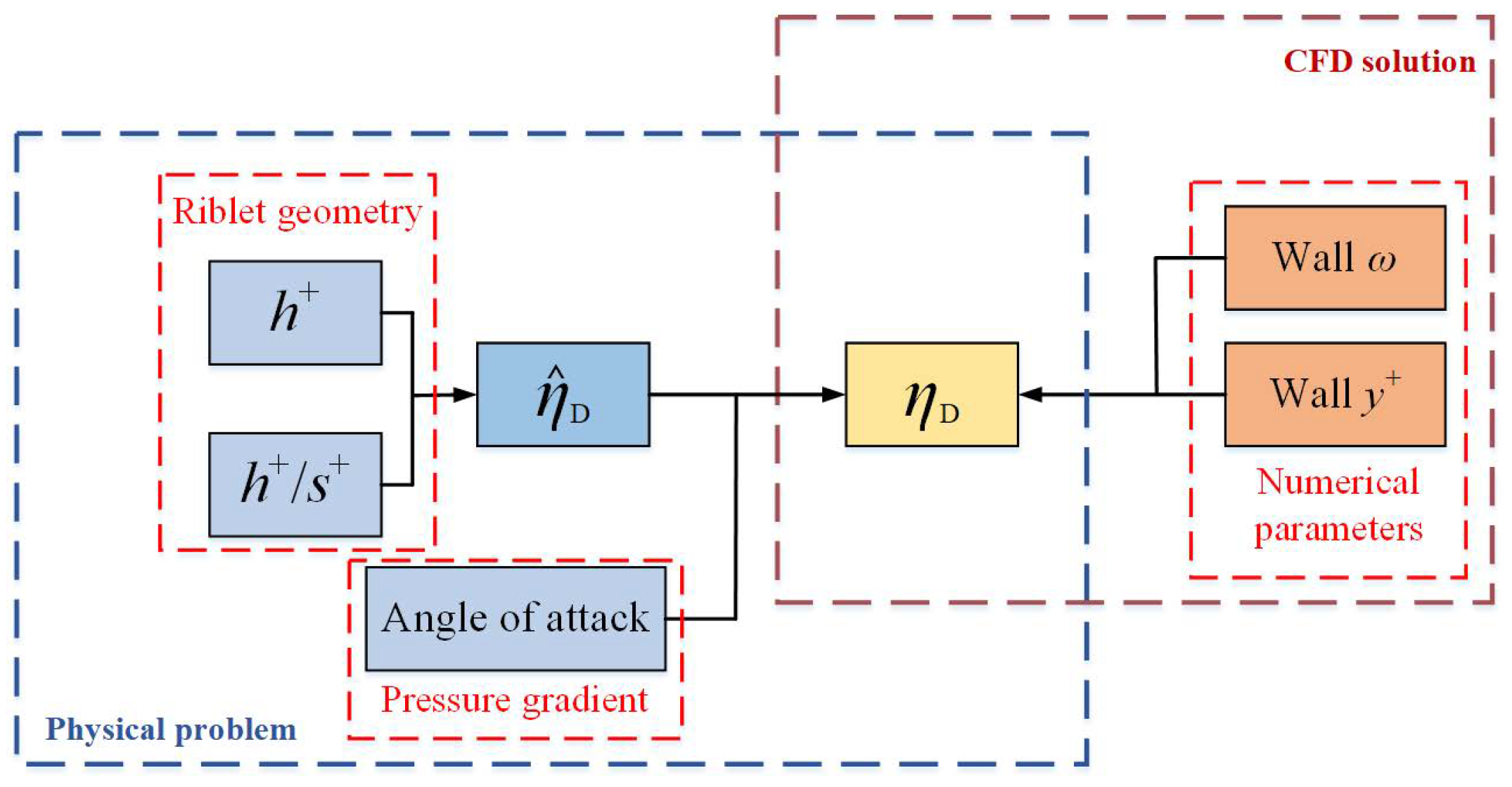
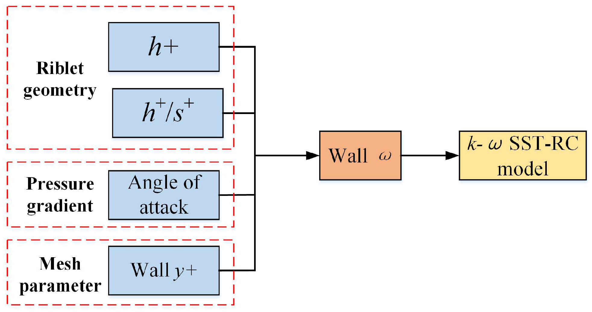
To simulate the performance of riblets on a body with curvature, a modified k- SST-RC model is constructed. The factors which can influence numerical results are gathered, and the relations between the factors and wall value of the SST k- model are constructed. Moreover, in this work, triangular streamwise riblets are used as an example to introduce the procedure of modifying the SST-RC model. Hence, the factors that are taken into account and their relationships are illustrated in Figure 1.
In Figure 1, denotes non-dimensional height of the riblets, denotes the non-dimensional spacing of the riblets, represents the drag reduction ratio without angle of attack, is the drag-reducing effect with the effect of angle of attack, namely the drag-reducing effect of practical configuration. Wall (denoted as ) represents the value of at wall boundary, and wall (denoted as ) is the value of at the wall boundary.
As shown in Figure 1, for the triangular riblets, the geometry parameters, and ratio, affect drag-reducing performance of the riblet surface. Hence, and need to be taken into account. In addition, pressure gradient effects must be considered, since the boundary layer of a three-dimensional wing–body configuration is affected by different pressure gradients and since it has demonstrated that pressure gradients can increase the drag-reducing effect of riblets [16,17]. For a practical configuration, angle of attack affects the pressure gradient, so the effects of the pressure gradient are assessed by angle of attack in this work.
For the k- SST model, Wilcox [25] proposed that the skin friction decreased with the increasing wall value. Once the wall is changed, wall distance of the computational grid, , will also affect the result of drag prediction. Based on this property, both and are taken into account to simulate the effect of riblets on viscous drag.
The Investigation of Choi et al. [9] demonstrated that the riblet surface could shift the logarithmic region, while the shape could be preserved. Compared with the smooth surface, the shift in the profile of the logarithmic region denotes the drag-decreasing case, while the overall decrease in the profile of the logarithmic region corresponds to the drag-increasing case. For a smooth wall, the profile of the logarithmic region is as follows:
where , , (the von Karman constant) is 0.41, and C is 5.2. To take into account the effects of shift on the logarithmic law, the profile for the riblet surface can be:
where denotes the additional velocity caused by riblets.
2.3. Steps to Modify the SST-RC Model
2.3.1. The Effect of Riblet Geometry
For the triangular riblets, the height and the ratio can determine the shape of the riblets; hence, the two parameters can affect the drag-reducing effects. To avoid the case where the final expression is complicated, the drag-reducing effect is defined as the ratio of drag acting on the riblets to drag corresponding to the flat surface, as follows:
where represents the drag reduction ratio without angle of attack, denotes the drag acting on the riblet surface without angle of attack, and denotes the drag corresponding to the flat surface. In this step, without the effect of angle of attack, the functional relationship between drag reduction and the riblet geometry shape factors is constructed, as follows:
where denotes the dimensionless height of the riblet, and represents the height to spacing ratio of the riblet.
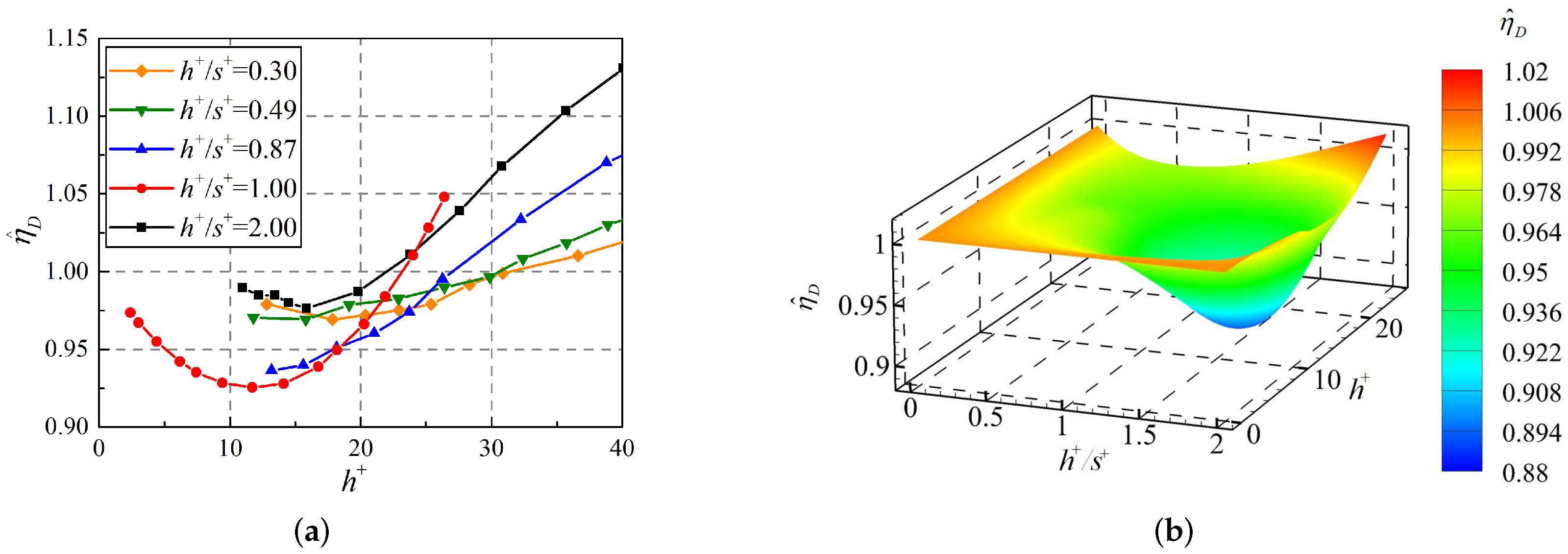
To build the relationship between the drag reduction ratio and the two parameters, the experimental data in [4,38,39] are used, as shown in Figure 2a. For the sake of simplicity, in Figure 2a, only a part of the data is illustrated. To construct the functional relationship, the cubic interpolation method is performed instead of the curve fitting. In the context of this work, there are two drawbacks to the curve fitting method, one is that the surface constructed by the curve fitting usually does not always hit the data points, and the other is that the scattered data points lead to a complex fitting function. By the interpolation technique, a curve (for one independent variable) or a surface (for two independent variables) through the data points is established, respectively. Consequently, at the data points, the function value is accurate.
Furthermore, there are concealed conditions. In the cases where , or , the riblet surface denotes the case of smooth surface, so the corresponding drag reduction ratio . Consequently, the function, , which is constructed by the cubic interpolation, is illustrated in Figure 2.
2.3.2. The Effect of Angle of Attack
In this work, the effect of angle of attack is considered to be a drag-reducing enhancement on the riblets in the cases where the airfoil are at angle of attack. As mentioned in Section 2.2, angle of attack is used as the direct parameter to construct the modified SST-RC model. The drag-reduction enhancement factor is defined as follows:
where denotes the angle of attack, and , the function of , denotes the factor in evaluating the improvement on the drag-reduction effect based on riblets. In this work, it is assumed that the drag-reducing effect is related to the angle of attack, which is similar for different configurations. Hence, considering only NACA 0012 data, and only between and angle of attack, this correlation is sufficient for demonstration purposes of the modelling approach presented in this work. Future work will focus on improving the model calibration by including data of a larger number of airfoils and a wider range of angles of attack.
where , and it denotes the drag reduction ratio of riblets with the effect of pressure gradient. Combined with Equation (9), can be determined, as follows:
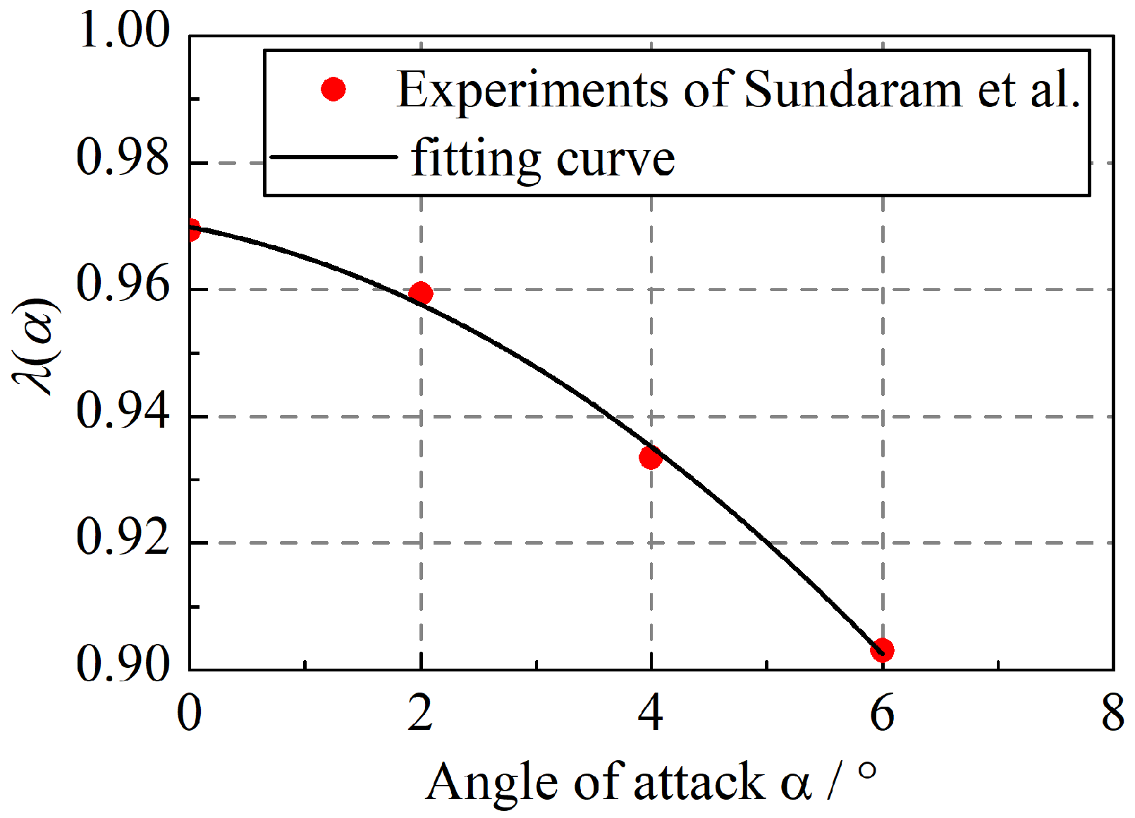
In this work, the data of NACA 0012 in [19] are used to establish the functional relationship, namely, the factor . Moreover, there is one important assumption. Although the drag-reducing enhancing effect is obtained by the data of NACA 0012 airfoil, the improvement in drag-reducing performance is considered to be the same for other configurations. The relationship between and can be found in Figure 3.
In this step, the curve fitting method is employed to construct the functional relationship between and . From the data points, a 2nd-polynomial fitting curve is constructed. The functional relationship is shown as follows:
Thus, the relationship between and is as follows:
Angle of attack is also an important parameter for an aircraft, so using angle of attack as a direct variable to establish the modified SST-RC model will simplify the calculation.
2.3.3. The Effect of Numerical Parameters
In Section 2.3.1 and Section 2.3.2, the parameters corresponding to the physical problem are considered. In this step, the factors in numerical simulations are discussed. In the SST-RC model, wall and of the computational mesh will also affect the results of the drag. The ratio of the modified to in the orginal SST-RC model is defined as:
where denotes the wall in the modified SST-RC model, and corresponds to that of the original SST-RC model.
Although the change of drag is caused by the modification of the numerical parameters, this can be regarded as a kind of drag-reducing effect. Hence, in numerical simulations, drag reduction ratio becomes the function of wall value and wall , as follows:
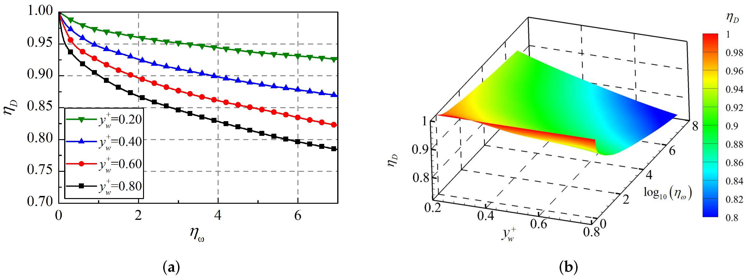
According to Li et al. [33], the functional relationship can be determined by numerical tests. In this work, the same method is conducted. A series of numerical simulation tests with different wall and wall are carried out. In this step, the channel flow model is used to construct the relationship between the drag and mesh. The domain size of the channel flow model is (streamwise, normal and spanwise), and the Reynolds number based on the half height of the channel is 5000. There are 121, 101 and 81 nodes in streamwise, normal and spanwise direction respectively. The numerical results are illustrated in Figure 4.
Consequently, the function is established. Furthermore, the function can be transformed into the following form:
From Equation (15) in Section 2.3.2, is the function of , , and ; hence, becomes the function of , , and , as follows:
Namely, in the modified solver, the factors, angle of attack, at wall and riblet geometry are introduced directly to modify wall in the k- SST-RC model, and the relationships in Figure 1 can be simplified, as shown in Figure 5.
This is the whole procedure to construct the riblet-equivalent model. Based on the steps, the relationship between wall value and the other variables, , , , and , can be constructed. The model can be applied to a three-dimensional model with a smooth surface to predict the aerodynamic characteristics corresponding to the ribleted one.
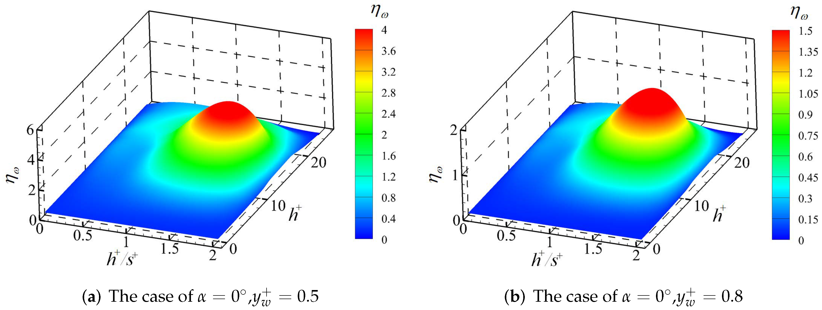
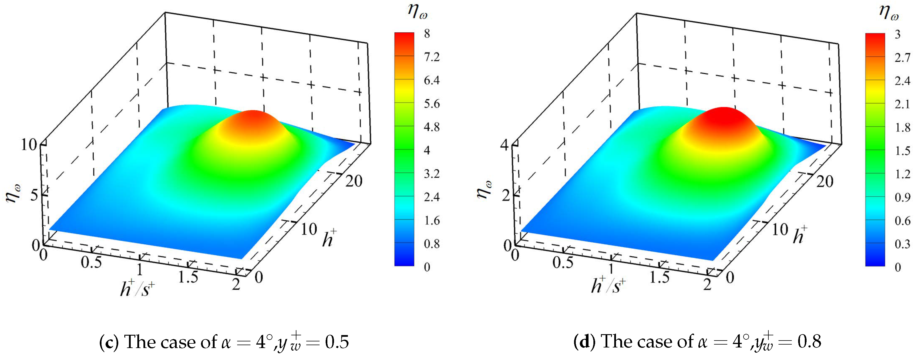
In some steps, the functional relationships are built using an interpolation method; therefore, the explicit expressions cannot be illustrated easily. The formulas have been embedded in the code of the solver, and Figure 6 illustrates the variation of with and at fixed and .
3. Validation
In this work, the CFD solver is OpenFOAM v2012, and the modified RANS model is combined with it. To validate the modified RANS model, the following three steps are used. Firstly, the original k- SST-RC model is verified by the NACA 0012 model and compared with the previous work in [40,41,42]. Secondly, by setting to 1.0, the model corresponds to the case of a zero pressure gradient flow (at angle of attack). Then, the results of drag reduction ratio and velocity profile are compared with those in [4,9,43]. Finally, the modified model where the pressure gradient factor is embedded is validated. In this case, NACA 0012 and GAW(2) airfoils, at different AoAs are studied, and the aerodynamic characteristics validated by the data in [19,20].
3.1. Validation of the k-ω SST-RC Model
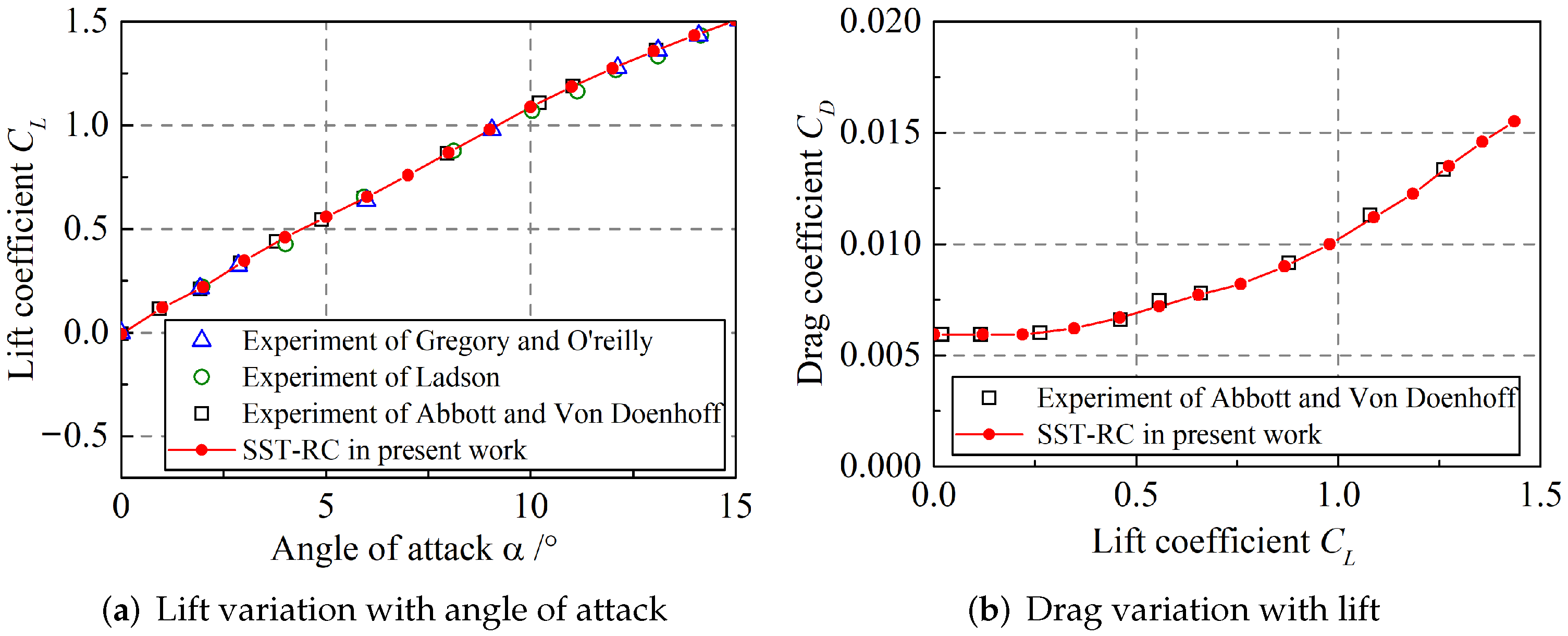
In this step, various aerodynamic data resources of NACA0012 airfoil are employed to validate the k- SST-RC model. The Reynolds number based on the chord length is . The O-type structured mesh is employed, and the mesh contains nodes in the chordwise and radial directions, respectively. The maximum dimensionless wall distance of the grid is 0.813. Because the solver is unstructured, the mesh will be converted into unstructured one before solving. The low-speed aerodynamic characteristics of NACA 0012 airfoil obtained using original k- SST-RC model are illustrated in Figure 7.
As reflected in Figure 7, the SST-RC model performs well in predicting aerodynamic forces at both lower and higher AoAs. Hence, the original SST-RC model is accurate and reliable to resolve the aerodynamic characteristics of a three-dimensional body at AoAs. Moreover, it is reasonable to use the SST-RC model as the baseline model where the modifications are conducted.
3.2. Validation of Riblet Flow without Angle of Attack
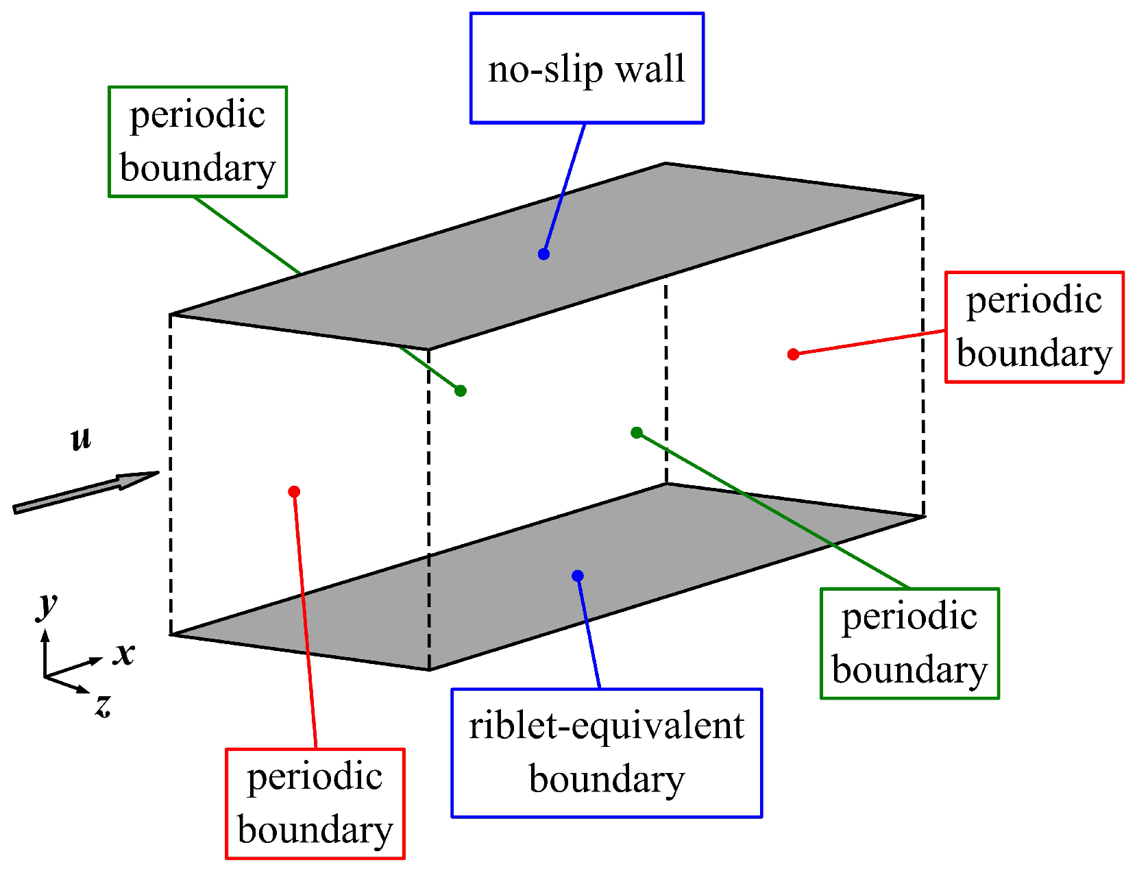
In this validation step, the velocity profiles on the flat surface and the riblet surface in [9,43] are used for verification purposes. Kim et al. [43] examined the fully developed turbulence bounded in a channel using the DNS method, where is 180. Choi et al. [9] utilized the channel model to investigate the turbulence statistics over riblets, where (based on the half-channel height), corresponding . To estimate the performance of the modified SST-RC model, the channel model is utilized. The walls are flat, and the riblet-equivalent boundary is employed, as shown in Figure 8.
Moreover, there is no effect of angle of attack in this numerical simulation. Namely, is set to 1.0 in this validation step. The results of drag-reducing effects are illustrated in Table 1.
Table 1 compares the results of the present work and previous work. It can be observed that the riblet-equivalent boundary condition is fairly accurate. Because the SST-RC model is modified according to the data in [4], the results accomplished through the modified SST-RC model will agree with the experimental data in [4]. Thus, after modifications, the SST-RC model is accurate in predicting the drag of riblets.
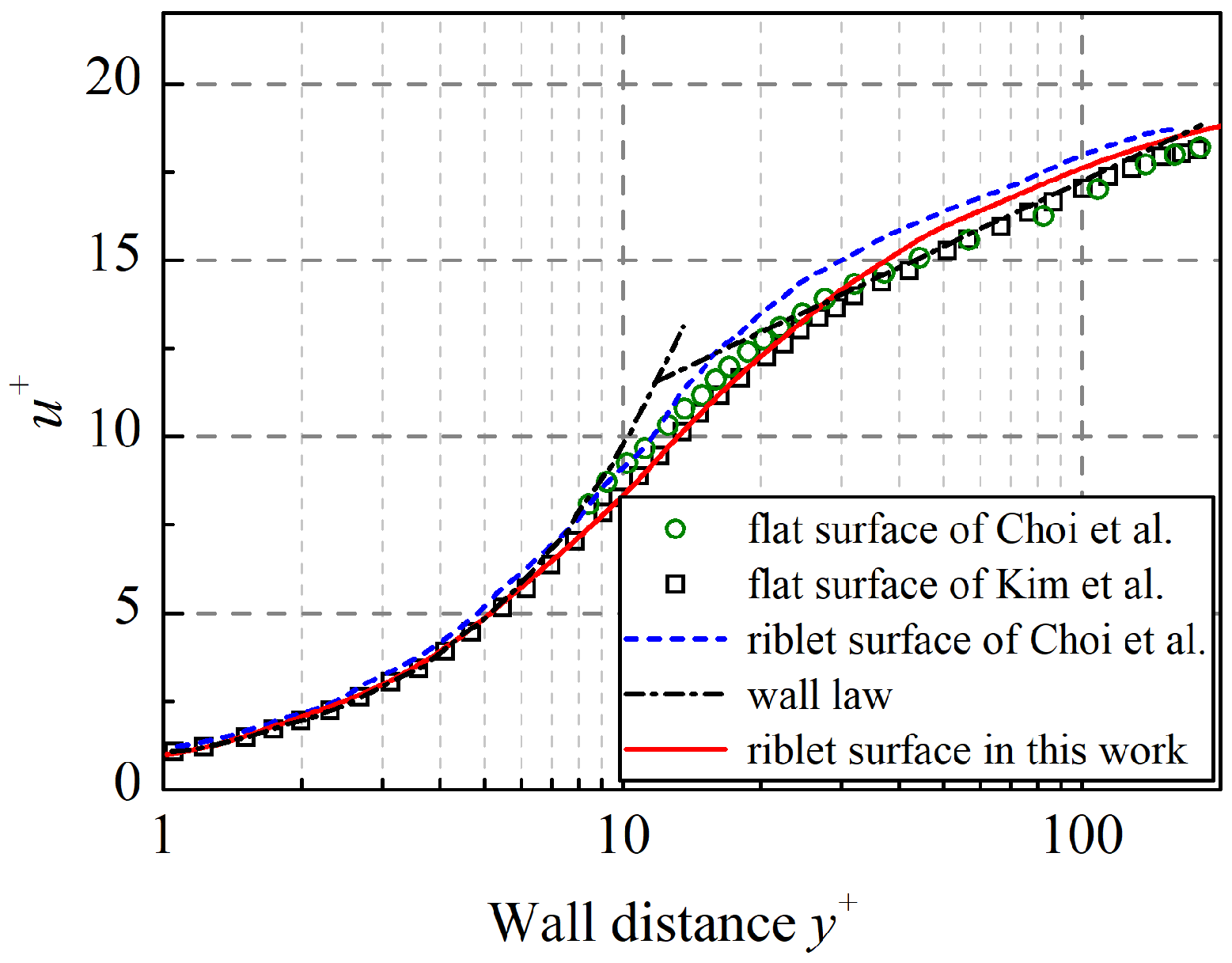
At the same time, the velocity profile in this work is compared with the previous work, as shown in Figure 9. For the logarithmical region in each case, the profile has the same slope (1/) but a different intercept. In addition, the shift of the intercept corresponds to drag reduction. As reflected in Figure 9, there is a shift in the logarithmical region for the velocity profiles. Moreover, the drag reduction ratio is 6.00%, according to the results of the work of Choi et al. [9], and the effect is 3.91% in the present work. The shift of logarithmical in present work is smaller than that in [9], and the logarithmical region is higher than that in the case of the flat plate.
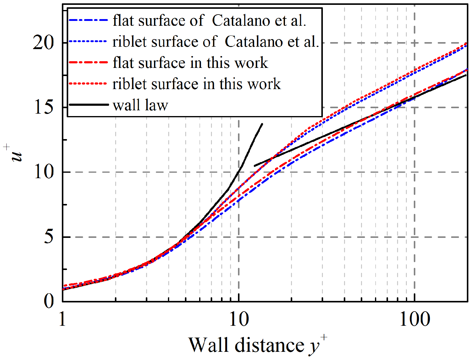
Then, the comparison work between the modified SST-RC model in this work and the numerical method of Catalano et al. [31] is conducted. In the work of Catalano et al. [31], a modified k-ω model is used to evaluate the flow over riblets, and the mean velocity profile on the riblet surface is compared with that of the flat plate. In [31], the single parameter is used, and , which corresponds to the maximum drag reduction ratio. In this work, two parameters, h+ and , are used, and the maximum drag-reducing effect is accomplished in the case of , which is corresponding to the case of in [31]. Then, the results of the simulation in this work and [31] are compared, as shown in Figure 10.
From the figure, it can be observed that the result of the modified RANS model in this work is in accordance to that in [31]. In this work, the drag reduction ratio is , a little lower than the ratio of 6% reported in [31]. As reflected in Figure 10, the shift in the logarithmic region is lower than that in [31], which is in agreement with the work of Catalano et al. [31]. Therefore, the comparison work illustrates that the modified SST-RC model performs well on predicting the velocity profile of the flat surface.
3.3. Validation of Riblet Flow with Angle of Attack
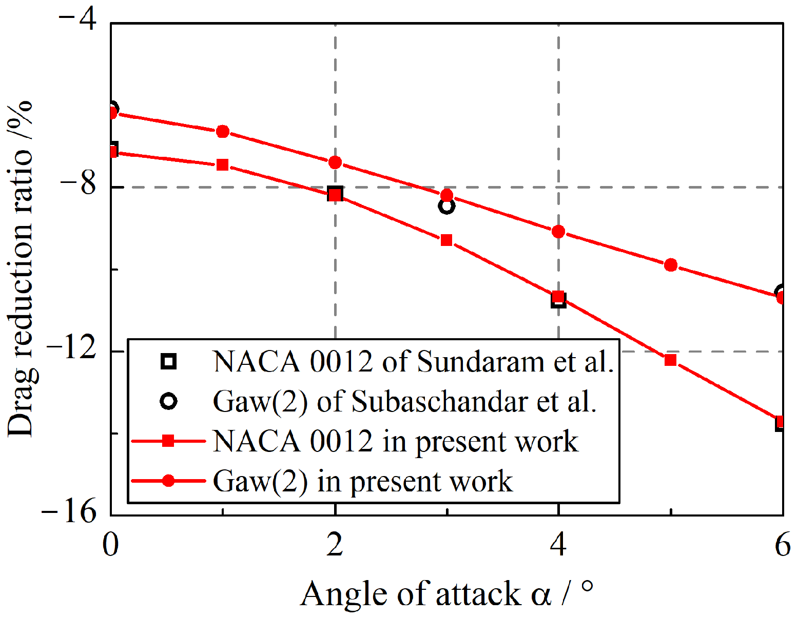
In this step, the drag characteristics of the airfoils in [19,20] are employed to test the modified SST-RC model. For the airfoils, the existence of angle of attack can maintain the drag-reducing effect of riblets. Sundaram et al. [19] measured the drag of ribleted NACA 0012 airfoil at different angles of attack, and Subaschandar et al. [20] examined the same phenomenon based on the ribleted GAW(2) airfoil. The results achieved by the modified SST-RC model in this work are compared with the two experimental studies, as demonstrated in Figure 11.
From Figure 11, the drag predicted by the modified model is accurate in both cases. For the NACA 0012 airfoil, the prediction of the drag-reducing effect is fairly accurate because the parameters in the SST-RC model are calibrated using the experimental results of NACA 0012 from studies in [19]. For a GAW(2) airfoil, a maximum error of predicting the drag reduction ratio is 3.00%, which is accomplished at AoA. Therefore, the modified SST-RC model is still of fine accuracy, although it is modified according to the drag-reducing performance of NACA 0012. Hence, within the angle of attack range used for calibration, the modified model is accurate for the simulation of the three-dimensional configurations.
4. Numerical and Experimental Investigations on a Wing–Body
In this section, the drag acting on a wing–body configuration is predicted by the modified k- SST-RC model. Then, an aerodynamic force measurement experiment is conducted to examine the effects of riblets. Subsequently, the aerodynamic drag is examined by experimental techniques, and the drag characteristics obtained by both methods are compared.
4.1. Details of the Practical Configuration
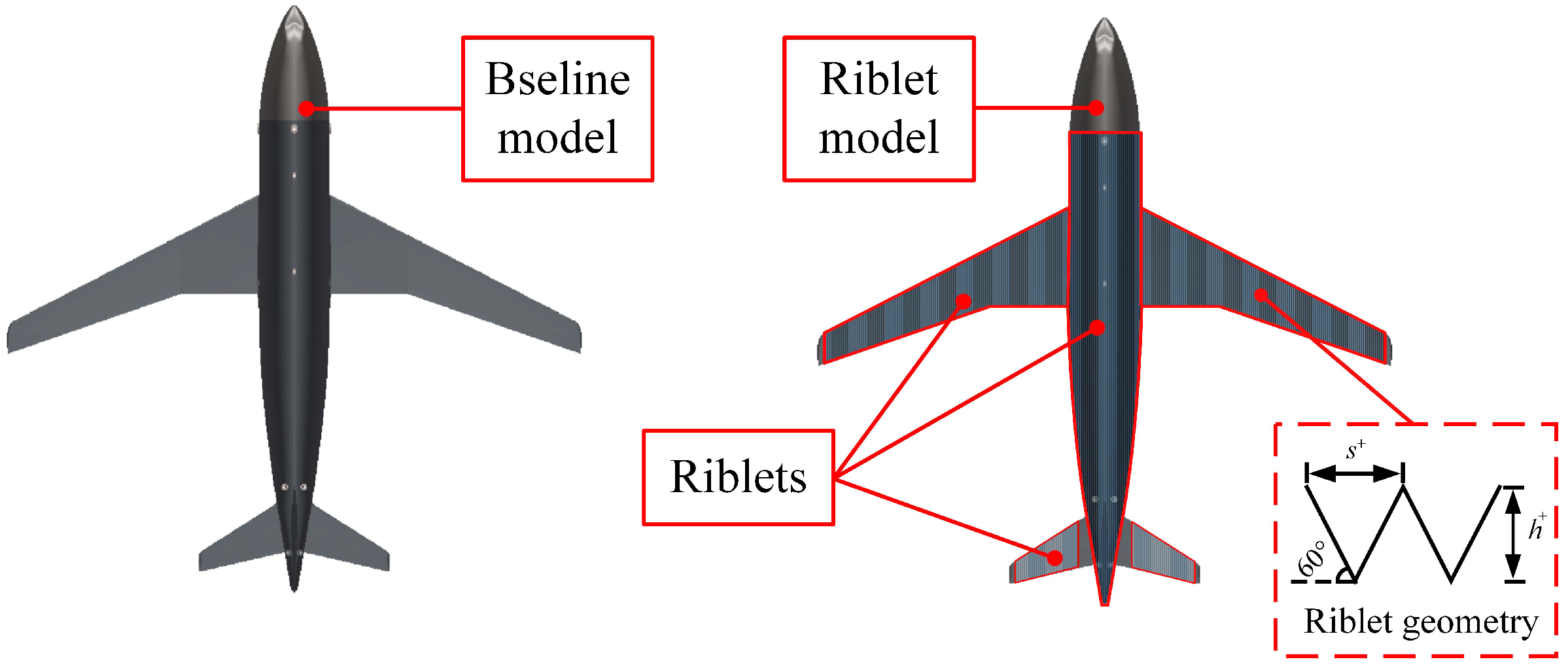
In this work, a wing–body configuration only has the fuselage, wings, horizontal stabilizer, and vertical stabilizer, as shown in Figure 12.
In this work, the size of the aircraft model in the numerical simulation and that in the experimental investigation are the same, and the detailed size of the model is illustrated in Table 2.
For the ribleted wing–body model in this work, most of the area of the fuselage, wings, and stabilizers are covered with riblets. For the riblet surface, the spacing is 0.41 mm. Because the ridge angle of the riblet is , . Then, the riblet height is supposed to be 0.36 mm. To adapt the change of cross-sectional shape along the body, the width of the riblet will be modified. Therefore, the spacing at the head of the body is 0.7 mm, and it is 0.30 mm at the end of body. The area covered with riblets is also illustrated in Figure 12.
4.2. Computational Details
4.2.1. Computational Domain
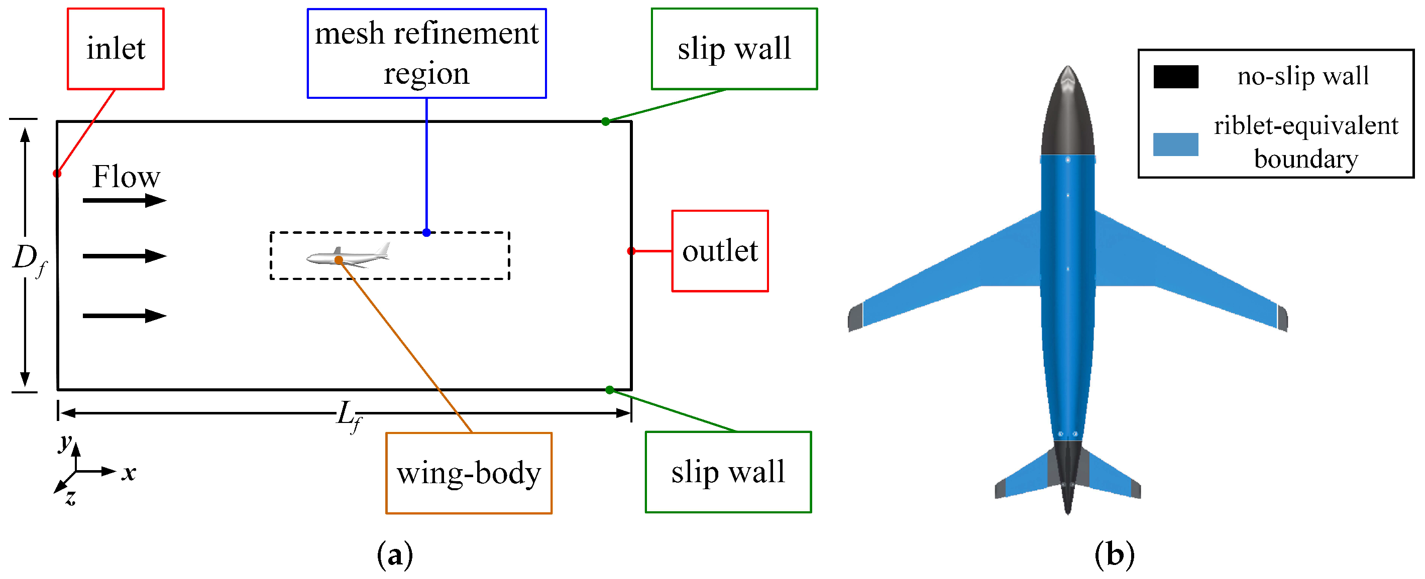
The far-field is of cylinder shape, the radius and height of which is 15 and 30 aircraft body lengths, respectively, as shown in Figure 13. Moreover, the unstructured mesh is used. At the body of the aircraft, in the area of riblets, the riblet-equivalent boundary condition and modified are employed, while the no-slip wall is employed for the smooth surface. At the inlet boundary, the velocity value is set to a fixed value, which is 25 m/s in this work, while the zero-gradient condition is used for pressure. At the outlet, the boundary condition of velocity is zero-gradient, while pressure value is set to a given value, which is 0 Pa. For the side wall, the slip-wall boundary is conducted. The riblet surface is a type of drag-reducing method for turbulent regime, and most of the surface of the wing–body configuration is mounted with riblets. Thus, the fully turbulent flow is assumed. In addition, for unseparated flow, according to Catalano et al. [31], there was no need for the treatment to predict separation location. Hence, in this work, no extra work on the prediction of the transition or separation location is conducted.
The flow direction can also affect the drag-reducing effect of riblets. In the case where there is non-ignorable spanwise flow in flow field, the riblet surface can be regarded as the directional riblet. According to Wu et al. [44], directional riblet surfaces can affect the turbulent/non-turbulent interface and modify the drag reduction ratio. For the modified RANS model in this work, it is assumed that there is no strong spanwise flow on the riblet. In addition, the speed of the wing–body configuration is low, and the there is no side-slip angle. Hence, in this work, the spanwise flow is ignorable and the modified SST-RC model can be applied.
The simulations were performed using a steady, incompressible solver. The Reynolds number, based on the main body length, is . For this Reynolds number, varied between 26 at the head and 18 in the tail region. The simulations were carried out on a cluster system consisting of AMD EPYC 7452 nodes, with 64 cores each. Using 10 cluster nodes in parallel required a calculation time of approximately 1.5 h to obtain a converged solution for the finest mesh of 7.95 million nodes.
4.2.2. Grid Independence Validation
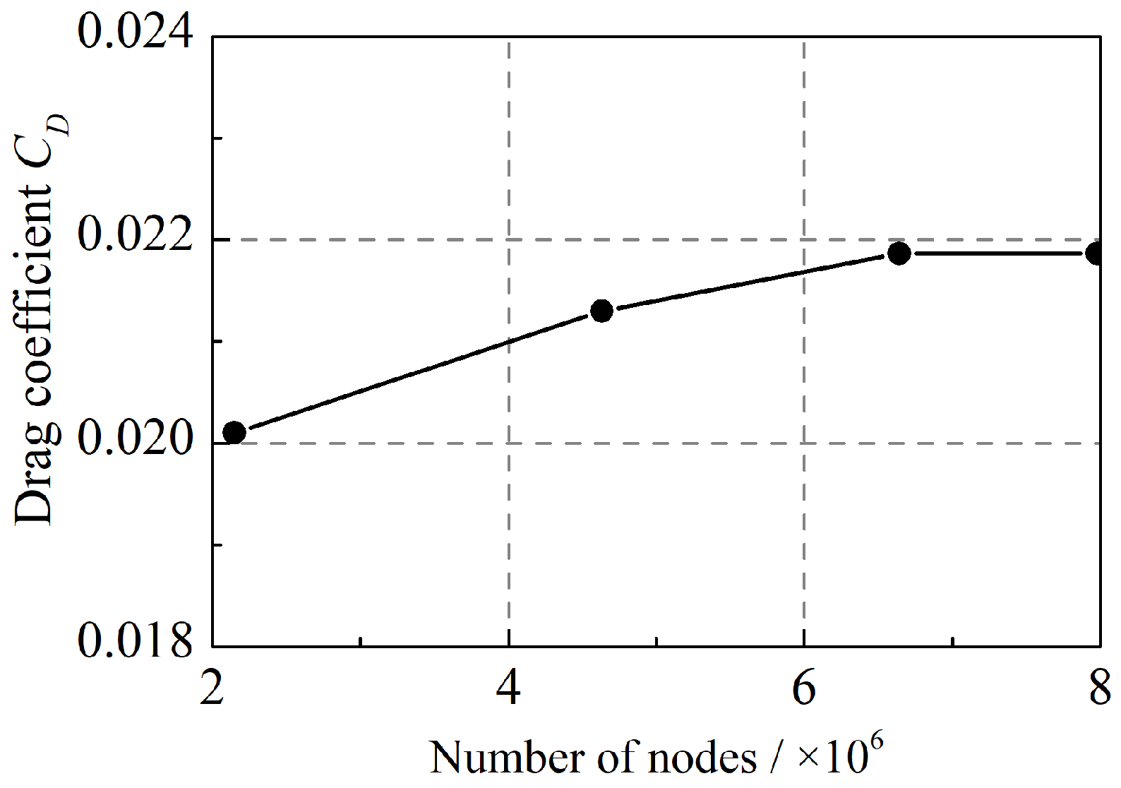
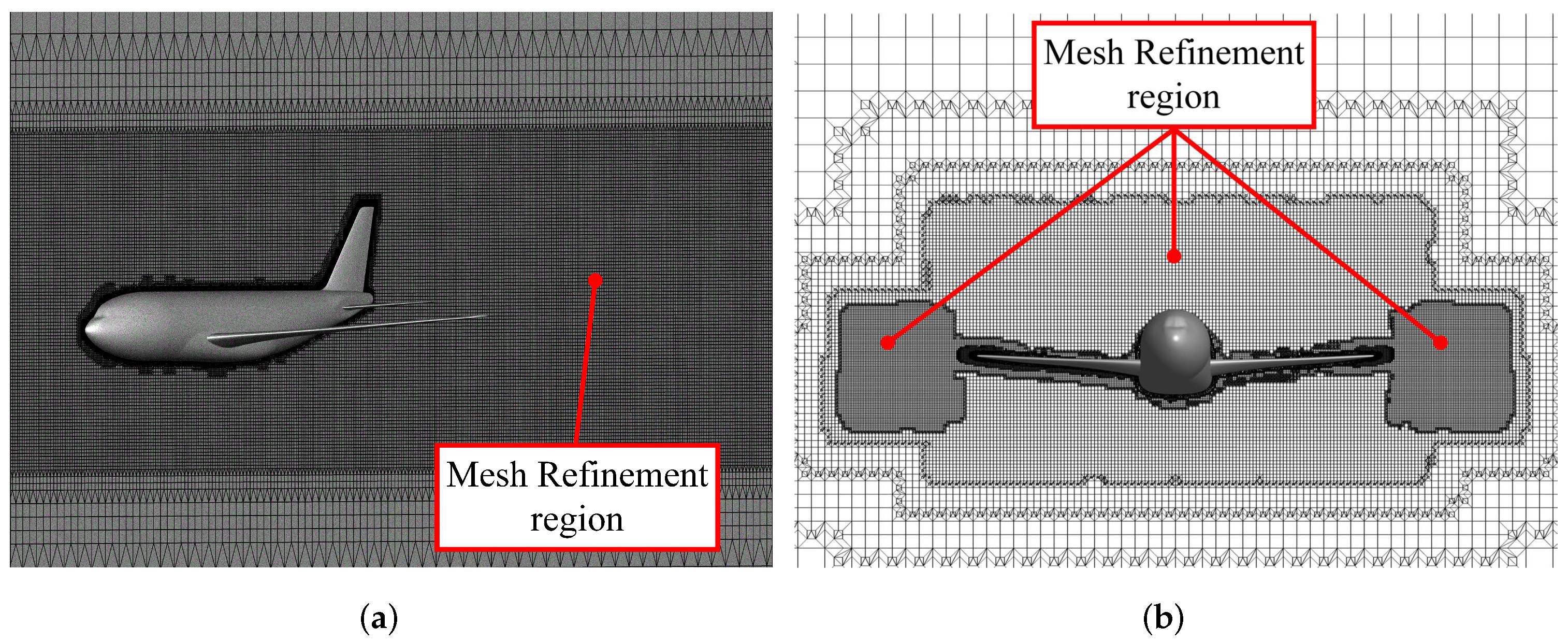
The grid resolution and the number of points can affect the results of the simulation. To ensure that the mesh is resolved enough in this numerical simulation, the grid independence is checked. The case where the angle of attack is is used for verification purposes. In this work, four sets of mesh are prepared, and the corresponding drag coefficients are demonstrated in Figure 14. In the grid independence validation, not only do the total nodes increase, but also the number of nodes in the near-wall region is also increased. In this work, the mesh in the region whose is lower than 500 is refined. For the cases in Figure 14, from the coarser mesh to the resolved mesh, the growth rates of the boundary layer mesh are 1.4, 1.3, 1.2, and 1.1, and the sizes of the surface mesh cells are decreased.
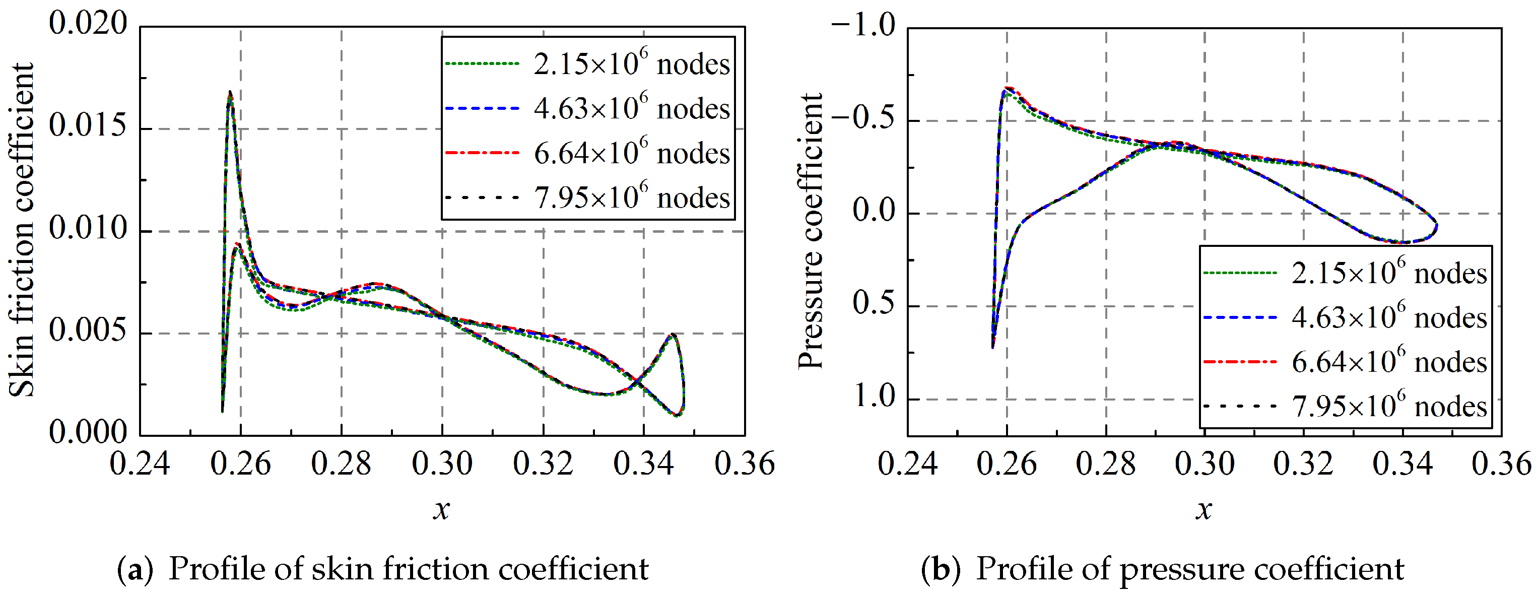
As reflected in Figure 14, the result of drag prediction is highly accurate, when the number of grids is larger than 6.64 million. In addition, a further comparison work is conducted. In this work, the skin friction coefficient and pressure coefficient on the cross section, which is 1/6 wing span to the wing root in each case, are illustrated, as shown in Figure 15.
From Figure 15a, it can be observed that there are differences between the distributions of skin friction coefficient obtained using coarser mesh and those obtained using refined mesh. For the distribution of the pressure coefficient in Figure 15b, the phenomenon is similar. Therefore, the increase in the number of nodes cannot cause the changes in the skin friction coefficient and pressure coefficient, when the number of nodes reaches 6.64 million. This indicates that the mesh which contains 6.64 million points is fine enough. Hence, all simulations in this work employ this set of the grid with 6.64 million points. The maximum for this mesh is 0.8571, and hexahedral cells are generated to resolve the boundary layer, as demonstrated in Figure 16.
4.2.3. Computational Results
The computation will be stopped, when the force coefficient converges or the magnitude of the residual becomes too small. In this work, the drag coefficient of the wing–body configuration is defined as:
where D corresponds to the aerodynamic drag; and are the fluid density and the flow velocity in the free stream, respectively; finally, represents the area of wings. Riblet performance can be assessed by introducing the drag reduction ratio, as follows:
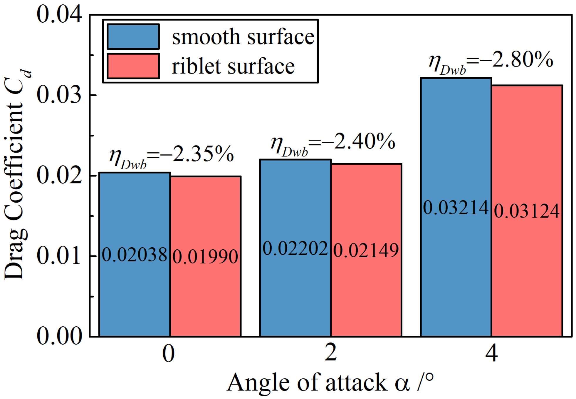
where denotes the drag acting on the baseline model, and represents the drag corresponding to the wing–body mounted with riblets. The results of drag coefficients and drag reduction performance are illustrated in Figure 17.
For the cases in the numerical work, the angle of attack is up to , which stays within the angle of attack range used for calibration. As shown in Figure 17, the drag-reducing effect is achieved, and drag reduction ratios are between 2% and 3%. It can be observed that the drag-reducing effect increases with the incline in AoA. It is noted that, in this work, data that are used to construct the riblet-equivalent boundary condition only contain the results where the angle of attack is up to . The functional relationship between drag-reducing enhancement and angle of attack in this work is based on the curve fitting method (Section 2.3.2). If the value of an input parameter is outside the scope of the dataset, which is used to calibrate the modified model, a larger error may be introduced.
4.3. Experimental Details
In this section, the drag of the wing–body is investigated by experimental techniques; moreover, drag-reducing effects are compared with the numerical prediction. A brief introduction of the experiment setup is shown; then, results of experimental examinations are shown.
4.3.1. Experimental Setup
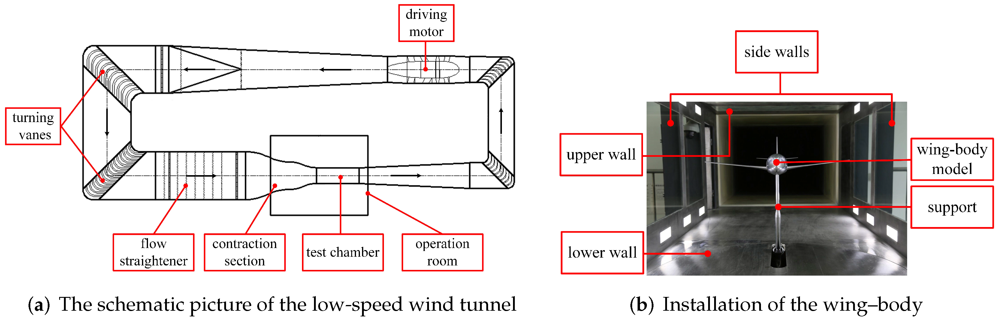
Experiments are carried out in a wind tunnel, and the airflow speed ranges between 20 m/s to 130 m/s. The wind tunnel has a 1.8 m × 1.4 m cross-section, where the pressure stability is 0.2%, and the turbulence intensity is 0.08%. The schematic plot of the wind tunnel is shown in Figure 18a. In experiments, the model is the same as that in the numerical simulation (Figure 12). In addition, two models are manufactured, and they are the smooth model and the riblet model. For the riblet one, the area where riblets are covered is the same as that in numerical simulations.
During the wind tunnel test, the internal six-component strain stress balance is used to obtain aerodynamic forces and moments of aircraft models. In addition, the balance is calibrated, so that the combined load can be resolved. In this work, the accuracy of the balance is better than a full scale. Each case is repeated three times. In this test, the wind speed is 25 m/s, and the pressure in the test chamber is 100,021 Pa; consequently, conditions are consistent with the numerical simulation.
4.3.2. Experimental Results
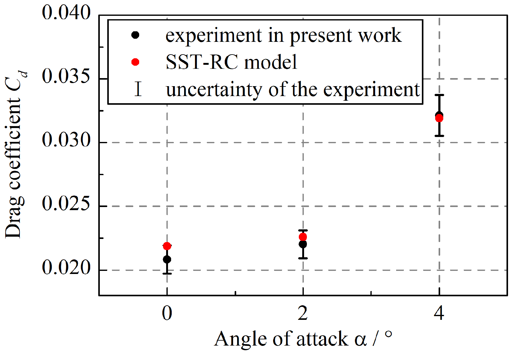
To evaluate the effectiveness of SST-RC turbulence model, comparison work between the drag coefficient obtained by the numerical simulation and that of the experimental investigation is conducted, as shown in Figure 19.
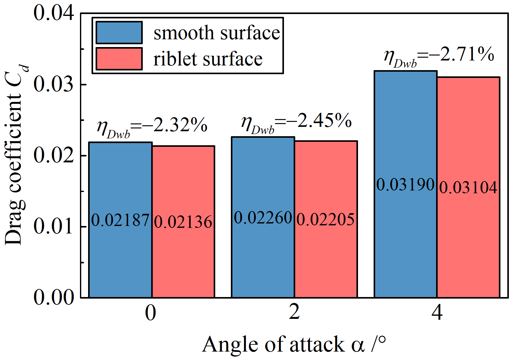
From Figure 19, it is can be observed that, for the drag coefficient, the numerical results are in accordance with experimental results. Thus, this indicates that the original SST-RC model used in this work is accurate. Furthermore, the aerodynamic drag characteristics of the smooth model and the ribleted model obtained by experiments are illustrated in Figure 20. It can be observed that the drag-reducing effect obtained by the experiment is between 2% and 3%; consequently, this is in good accordance with the numerical result.
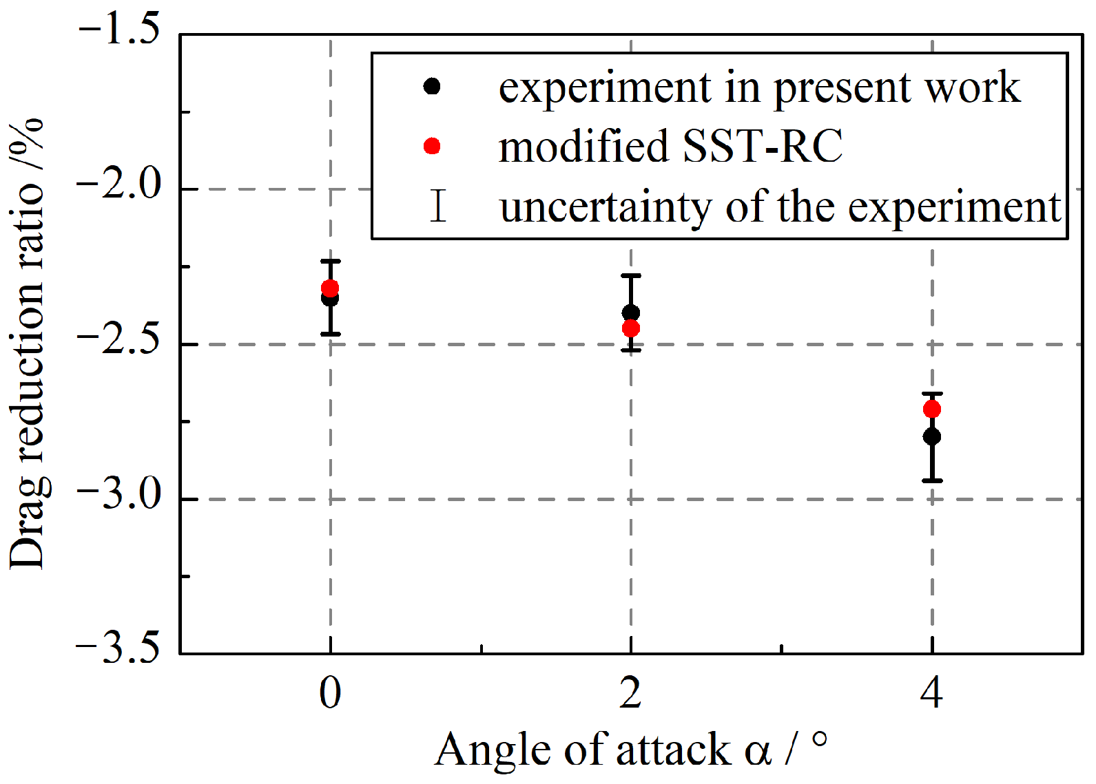
Compared with the numerical simulations in Figure 17, the experimental results illustrate that the original SST-RC model is accurate in predicting the drag of a three-dimensional body. Furthermore, the drag reduction ratio of riblets obtained by numerical methods and experimental investigations are compared and shown in Figure 21.
As reflected in Figure 21, both numerical and experimental investigations demonstrate that the riblets can reduce the drag of a three-dimensional configuration. Numerical results obtained by the modified SST-RC model agree with the results of experiments. Moreover, the maximum difference between drag reduction ratios obtained by numerical simulations and those obtained by experiments is 3.21%, which is lower than 5%. Hence, the modified SST-RC model is accurate in predicting the drag reduction for the wing–body configurations.
5. Analysis of Numerical Results
For the sake of simplicity, results of numerical investigations at are discussed in this section. In addition, drag components, skin friction distributions, and pressure coefficient distributions are illustrated and analyzed.
5.1. Drag Components
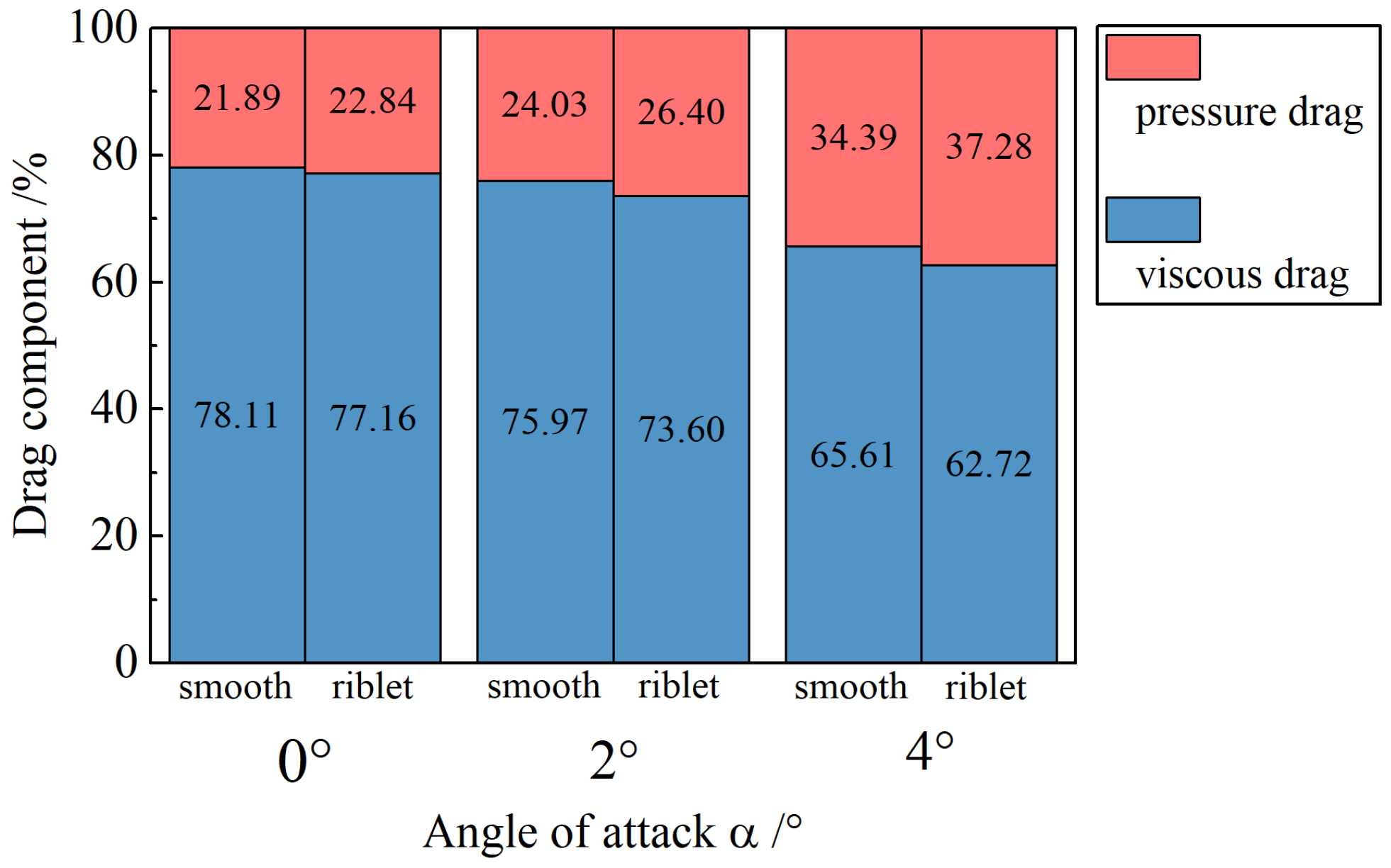
Drag can be divided into two parts, pressure drag and viscous drag. At low-speed and low-AoA states, the proportion of viscous drag is much larger than the pressure drag. In this part, the pressure drag and viscous drag are separated out from the total drag that is obtained by numerical simulations. The share of pressure drag and viscous drag in each case is shown in Figure 22.
At a low-speed state, the viscous-drag component of the total drag suppresses the pressure drag. As demonstrated in Figure 22, the proportion of the viscous drag decreases with the increase in the angle of attack in each case. For the wing–body mounted with riblets, there is an increase in the proportion of the pressure drag.
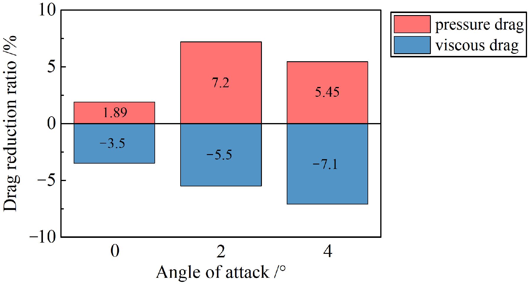
From Figure 22, in each case, there is a decrease in the viscous drag, while the pressure-drag component increases. The combination of the two opposite effects is responsible for the decrease in total drag. This tendency is also consistent with that in the work in [21]. To show the drag-reducing effect of riblets clearly, the drag reduction ratios of the viscous- and pressure-drag components are illustrated in Figure 23.
According to the numerical results in this work, with the increase in angle of attack, the viscous drag reduction ratio is inclined, while the pressure drag-increasing ratio increases. Furthermore, a maximum of 7.1% reduction in viscous drag is accomplished at AoA. The viscous component is larger than the pressure drag; hence, this contributes to the reduction in total drag.
5.2. Skin Friction Coefficient Distribution
In this investigation, the speed or the angle of attack is not too large, and the viscous drag accounts for a substantial part of the total drag. Hence, it is important to include an analysis of the proportion of friction drag in total drag. Furthermore, the skin friction coefficient is defined as follows:
where represents the wall shear stress, as follows:
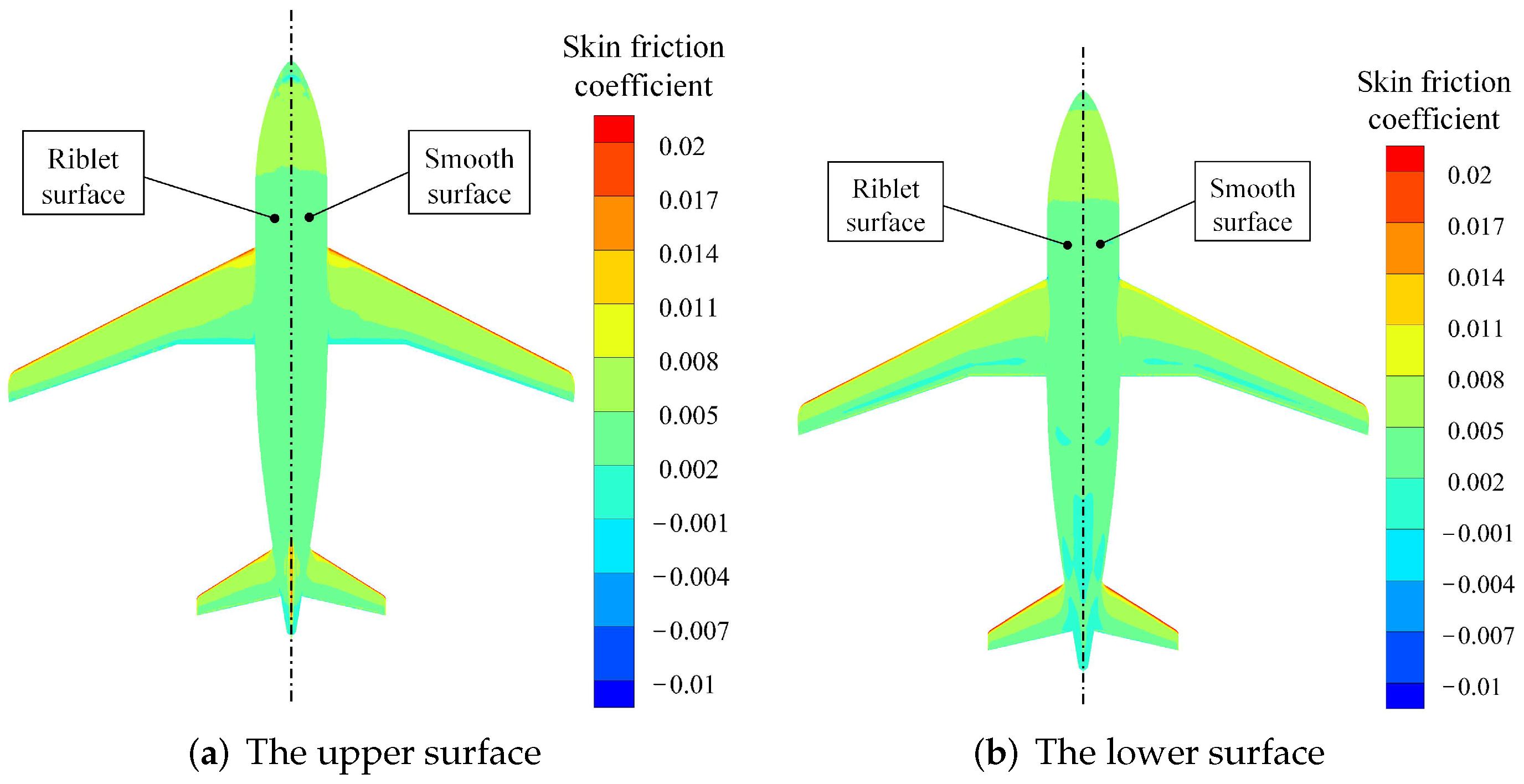
A comparison of the distribution of skin friction coefficient on the ribleted model with that on the smooth one is shown in Figure 24.
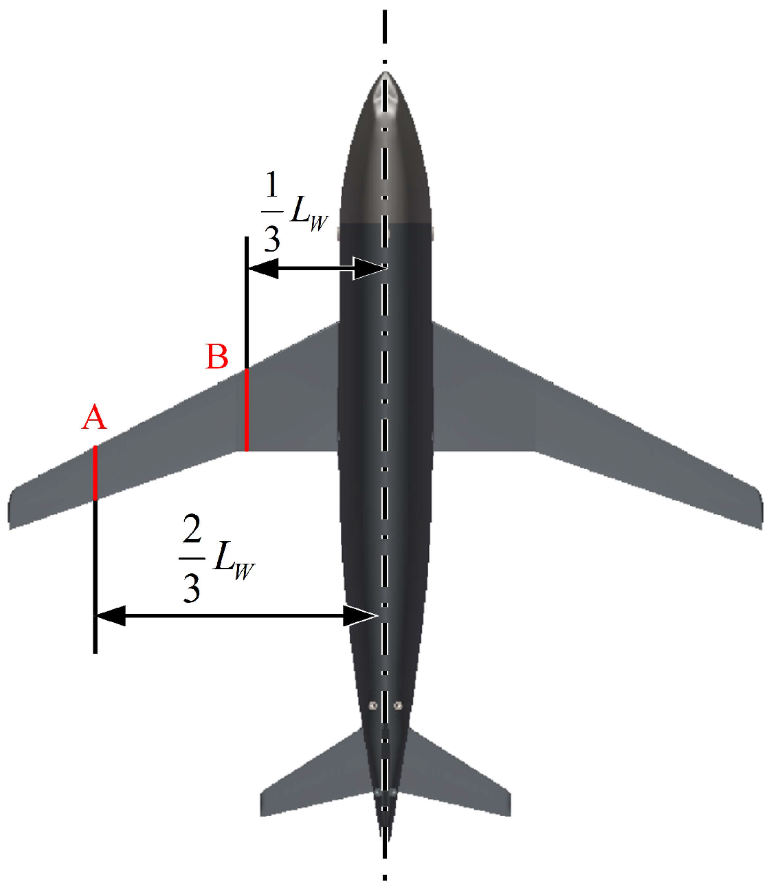
From the figure, the skin friction coefficient on a riblet model is slightly different from the smooth surface, and the friction coefficient at some positions is suppressed by that on the smooth one. To show the distribution of skin friction coefficient clearly, profiles at two cross-sections of the wings are demonstrated and compared. The positions of the cross-sections are illustrated in Figure 25.
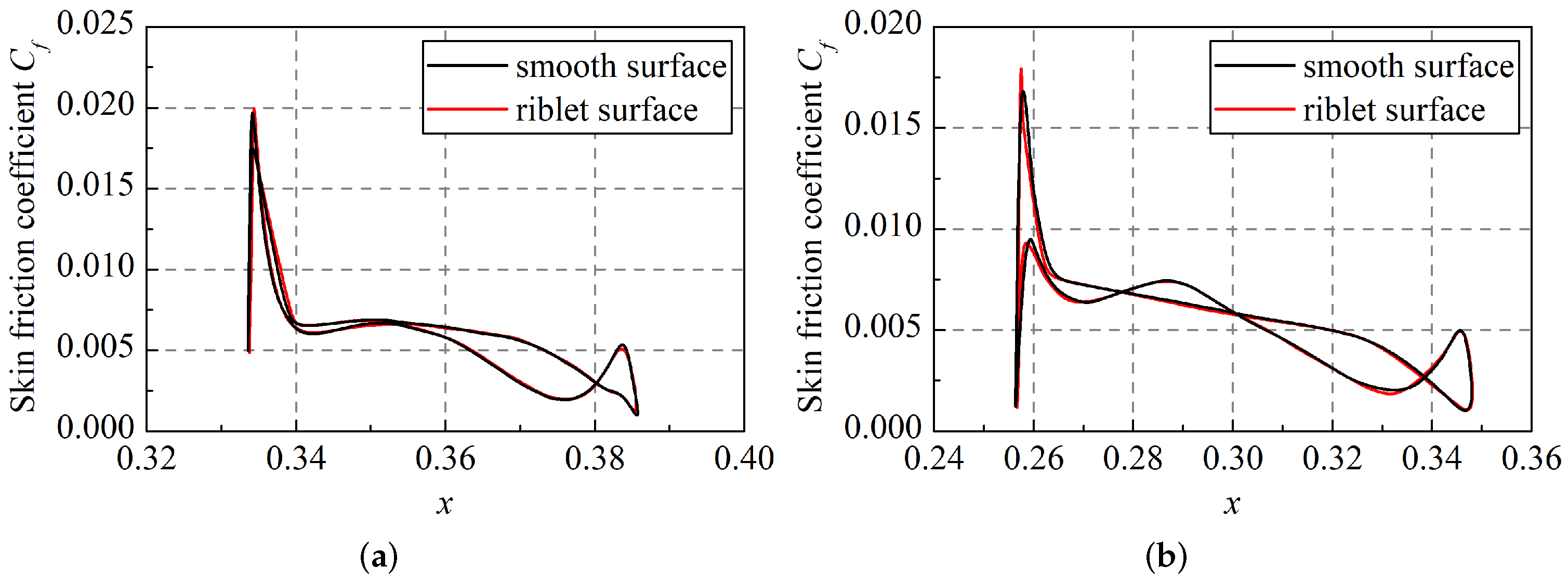
The wing, as an important component of the aircraft, affects the aerodynamic characteristics. For the two positions, one is near the wing root, and the other is close to the wingtip. The distributions of on the two airfoils of the wings are illustrated in Figure 26.
As shown in Figure 26, an overall decrease in the skin friction coefficient is accomplished. In addition, by comparing the distributions of the skin friction coefficient on the riblet model and the smooth model, there is a maximum of 5.36% decrease in the skin friction coefficient for the riblet model. For the ribleted model, although there is an increase in the skin friction at the leading edge, the skin friction coefficient on most area is lower than that of the smooth one. Because the modified SST-RC is constructed based on the principle that riblets shift the boundary layer (Figure 11), wall shear stress and skin friction obtained by the method will be lower. The distribution of skin friction coefficient agrees with the assumption.
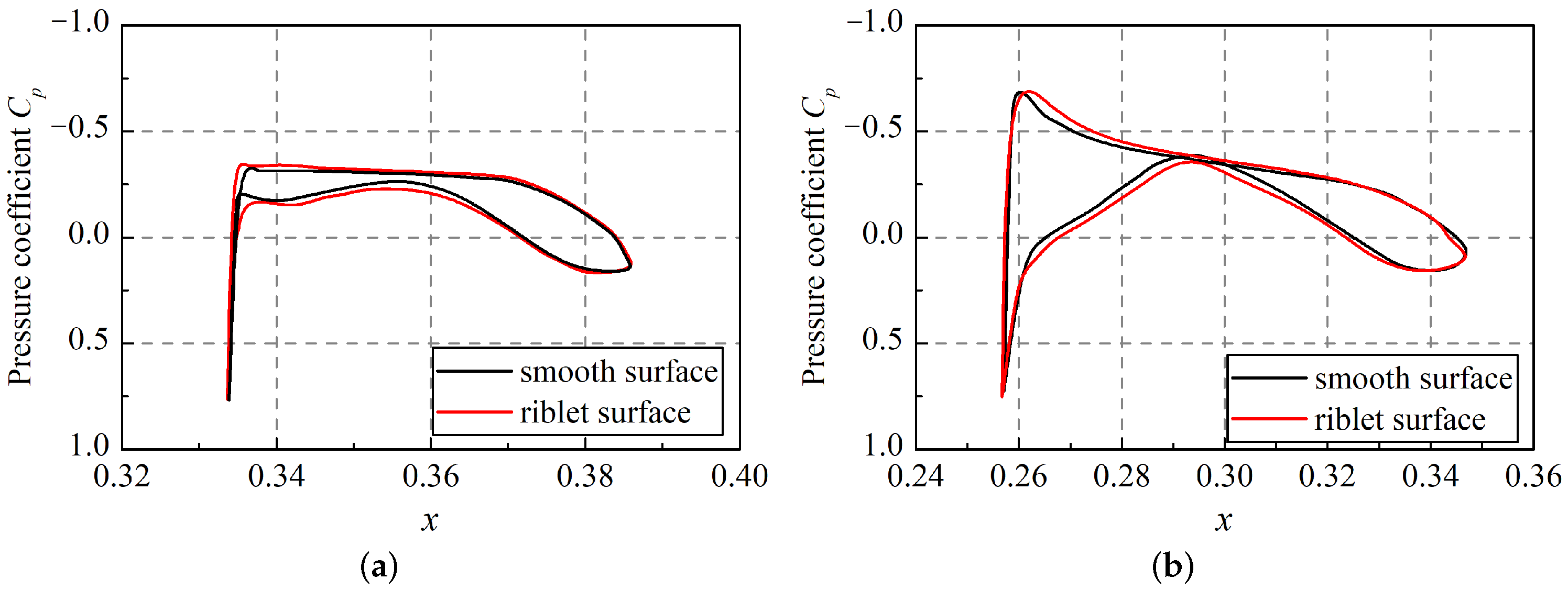
5.3. Pressure Distribution
With the incline in the angle of attack, the change of pressure distributions affects the aerodynamic characteristics of the wing–body more. Moreover, the contribution of the pressure drag to the total drag increases. Hence, the pressure drag cannot be ignored, and discussions on the pressure distribution are also illustrated in this section. The pressure coefficient is defined as follows:
where p denotes pressure at the point where the pressure coefficient is estimated; represents the static pressure in the free stream.
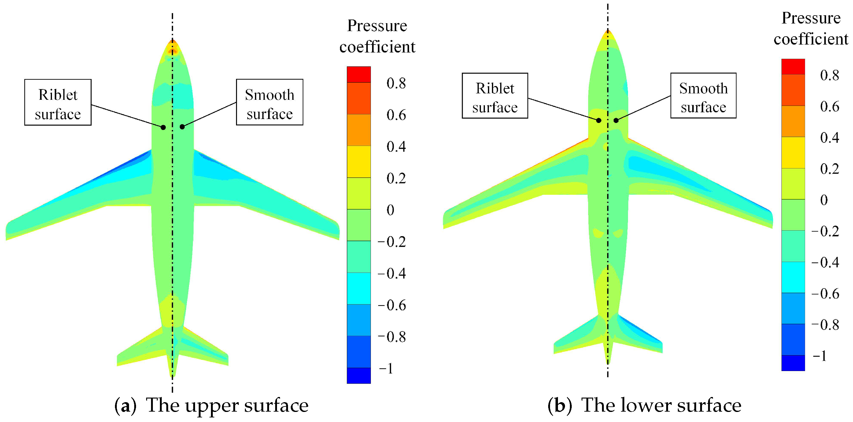
According to [21], LES simulations suggested that the riblet surface could modify the pressure field, which caused the change of aerodynamic characteristics. In this work, the pressure field is also modified due to riblets. The comparison of the pressure fields in both cases is illustrated in Figure 27.
As shown in Figure 27, in general, for the upper surface, the pressure in the ribleted case is lower than that in the smooth case. For the lower surface, compared with the smooth case, there is a slight increase in the pressure in the ribleted case. To show the distribution clearly, the same cross-sections on the wing shown in Figure 25 are chosen, and pressure coefficient profiles are illustrated in Figure 28.
From Figure 28, at the two cross-sectional profiles of the wing, effects of riblets on pressure distributions are similar. There is a decrement in pressure at the leading edge of the upper surface. In addition, for the lower surface, there is an increment in the pressure coefficient at the leading edge. However, only a slight modification in the pressure coefficient at the trailing edge of wings can be observed.
6. Discussion and Conclusions
In this work, the SST-RC model is modified to evaluate the drag acting on a practical configuration. The riblet-equivalent boundary condition makes it possible to estimate the drag of a three-dimensional body mounted with riblets through a smooth model, which lowers the computational cost. Furthermore, the main conclusions are shown as the following:
- The riblet-equivalent boundary condition combined with the k- SST-RC model is constructed. In the modified RANS model, the effect of pressure gradient on drag-reducing performance is taken into account, so that the method can be used for the case where there is system curvature and pressure gradient. Comparisons with the previous data illustrate that the modified k- SST-RC model can predict the drag precisely, and the maximum error is 3.00%.
- The results of numerical simulations on the wing–body model are consistent with the corresponding aerodynamic drag measurements, and a maximum error of 3.21% is achieved. The numerical simulations illustrate that a maximum of 2.71% drag-reducing effect is achieved at AoA. This demonstrates that the modified SST-RC model is accurate and can be applied to the drag prediction of the practical configuration.
- Analysis of numerical simulations demonstrates that, with the incline in angle of attack, there is a decrease in the viscous drag while the pressure–drag component increases. For the skin friction coefficient, there is an overall decrease on the riblet surface. In addition, distributions of the pressure coefficient are also modified.
Although some results have been accomplished based on the modification procedures, there are still drawbacks. Errors may be caused if the modified SST-RC model is applied beyond the range of the angles of attack which are used to calibrate the RANS model. In addition, the error may be generated while there is separation in flow field. In future work, our group will focus on solving the existing disadvantages. Our group will combine further experimental investigations with the numerical simulations to construct a more general RANS model for riblet-equivalent boundary conditions.
Author Contributions
Conceptualization and methodology, C.L.; software, S.T.; validation, C.L.; formal analysis, S.T.; investigation, Z.G.; resources, Y.L.; data curation, Z.G.; writing—original draft preparation, C.L.; writing—review and editing, S.T.; visualization, C.L.; supervision, S.T.; project administration, Y.L. All authors have read and agreed to the published version of the manuscript.
Funding
This research received no external funding.
Data Availability Statement
Not applicable.
Conflicts of Interest
The authors declare no conflict of interest.
Abbreviations
The following abbreviations are used in this manuscript:
| Latin characters | |
| Angle of attack | |
| Cross-diffusion term in the k- SST model | |
| Drag coefficient | |
| Drag coefficient of ribleted wing–body | |
| Drag coefficient of smooth wing–body | |
| Skin friction coefficient | |
| Lift coefficient | |
| Pressure coefficient | |
| Empirical constants in k- SST-RC model | |
| D | Aerodynamic drag |
| Drag of riblets without the effect of pressure gradient | |
| Drag acting on flat surface | |
| Dissipation term of -equation | |
| Dimensionless riblet height | |
| k | Turbulence kinetic energy |
| Length of the body of wing–body | |
| Span length of wings of wing–body | |
| Production term of turbulence kinetic energy | |
| Reynolds number | |
| Area of wing of the wing–body | |
| Dimensionless riblet spacing | |
| Three components of mean velocity | |
| Friction velocity | |
| Dimensionless velocity | |
| Additional velocity introduced by riblets | |
| Flow velocity of the free stream | |
| Three coordinates in space | |
| Cartesian coordinates | |
| Wall distance in wall unit | |
| Dimensionless wall distance of computational grid at the wall | |
| Greek characters | |
| Empirical constants in the k- SST model | |
| Angle of attack | |
| Dissipation rate of the turbulent kinetic energy | |
| Tensor of Levi–Civita | |
| Drag-reducing ratio with the effect of pressure gradient | |
| Drag-reducing ratio without the effect of pressure gradient | |
| Drag-reducing ratio of riblets on wing–body | |
| Ratio of to | |
| The von Karman constant | |
| Drag-reducing enhancing factor | |
| Dynamic viscosity | |
| Effective viscosity () | |
| Turbulent viscosity | |
| Kinematic viscosity | |
| Fluid density | |
| Fluid density in free stream | |
| Wall shear stress | |
| Turbulence eddy frequency | |
| Value of at wall | |
| Wall value of the modified SST-RC model | |
| Wall value of the original SST-RC model | |
| Vorticity tensor | |
| Components of | |
| Components of system rotation vector |
References
- Abu Salem, K.; Cipolla, V.; Palaia, G.; Binante, V.; Zanetti, D. A Physics-Based Multidisciplinary Approach for the Preliminary Design and Performance Analysis of a Medium Range Aircraft with Box-Wing Architecture. Aerospace 2021, 8, 292. [Google Scholar] [CrossRef]
- Walsh, M.J. Riblets as a viscous drag reduction technique. AIAA J. 1983, 21, 485–486. [Google Scholar] [CrossRef]
- Walsh, M.J. Effect of detailed surface geometry on riblet drag reduction performance. J. Aircr. 1990, 27, 572–573. [Google Scholar] [CrossRef]
- Walsh, M. Turbulent boundary layer drag reduction using riblets. In Proceedings of the 20th Aerospace Sciences Meeting, Orlando, FL, USA, 11–14 January 1982; p. 169. [Google Scholar]
- Luchini, P.; Manzo, F.; Pozzi, A. Resistance of a grooved surface to parallel flow and cross-flow. J. Fluid Mech. 1991, 228, 87–109. [Google Scholar] [CrossRef]
- Vukoslavcevic, P.; Wallace, J.; Balint, J.L. Viscous drag reduction using streamwise-aligned riblets. AIAA J. 1992, 30, 1119–1122. [Google Scholar] [CrossRef]
- Bruse, M.; Bechert, D.W.; van der Hoeven, J.; Hage, W.; Hoppe, G. Experiments with Conventional and with Novel Adjustable Drag Reducing Surfaces. In Proceedings of the International Conference on Near-Wall Turbulent Flows, Tempe, AZ, USA, 15–18 March 1993. [Google Scholar]
- Chu, D.C.; Karniadakis, G.E. A direct numerical simulation of laminar and turbulent flow over riblet-mounted surfaces. J. Fluid Mech. 1993, 250, 1–42. [Google Scholar] [CrossRef] [Green Version]
- Choi, H.; Moin, P.; Kim, J. Direct numerical simulation of turbulent flow over riblets. J. Fluid Mech. 1993, 255, 503–539. [Google Scholar] [CrossRef]
- Goldstein, D.; Handler, R.; Sirovich, L. Direct numerical simulation of turbulent flow over a modeled riblet covered surface. J. Fluid Mech. 1995, 302, 333–376. [Google Scholar] [CrossRef]
- Garcia-Mayoral, R.; Jimenez, J. Hydrodynamic stability and breakdown of the viscous regime over riblets. J. Fluid Mech. 2011, 678, 317–347. [Google Scholar] [CrossRef]
- Zhang, Z.; Zhang, M.; Cai, C.; Kang, K. A general model for riblets simulation in turbulent flows. Int. J. Comput. Fluid Dyn. 2020, 34, 333–345. [Google Scholar] [CrossRef]
- Wu, Z.; Yang, Y.; Liu, M.; Li, S. Analysis of the influence of transverse groove structure on the flow of a flat-plate surface based on Liutex parameters. Eng. Appl. Comp. Fluid 2021, 15, 1282–1297. [Google Scholar] [CrossRef]
- Li, W. Turbulence statistics of flow over a drag-reducing and a drag-increasing riblet-mounted surface. Aerosp. Sci. Technol. 2020, 104, 106003. [Google Scholar] [CrossRef]
- Li, C.; Tang, S.; Li, Y.; Geng, Z. Numerical and experimental investigations on drag-reducing effects of riblets. Eng. Appl. Comp. Fluid 2021, 15, 1726–1745. [Google Scholar] [CrossRef]
- Debisschop, J.; Nieuwstadt, F. Turbulent boundary layer in an adverse pressure gradient-effectiveness of riblets. AIAA J. 1996, 34, 932–937. [Google Scholar] [CrossRef]
- Nieuwstadt, F.; Wolthers, W.; Leijdens, H.; Prasad, K.K.; Schwarz-van Manen, A. The reduction of skin friction by riblets under the influence of an adverse pressure gradient. Exp. Fluids 1993, 15, 17–26. [Google Scholar] [CrossRef]
- Jung, Y.C.; Bhushan, B. Biomimetic structures for fluid drag reduction in laminar and turbulent flows. J. Phys. Condens. Matter 2009, 22, 035104. [Google Scholar] [CrossRef]
- Sundaram, S.; Viswanath, P.R.; Rudrakumar, S. Viscous drag reduction using riblets on NACA 0012 airfoil to moderate incidence. AIAA J. 1996, 34, 676–682. [Google Scholar] [CrossRef]
- Subaschandar, N.; Kumar, R.; Sundaram, S. Drag reduction due to riblets on a GAW (2) airfoil. J. Aircr. 1999, 36, 890–892. [Google Scholar] [CrossRef]
- Zhang, Y.; Chen, H.; Fu, S.; Dong, W. Numerical study of an airfoil with riblets installed based on large eddy simulation. Aerosp. Sci. Technol. 2018, 78, 661–670. [Google Scholar] [CrossRef]
- Boomsma, A.; Sotiropoulos, F. Riblet drag reduction in mild adverse pressure gradients: A numerical investigation. Int. J. Heat Fluid Flow 2015, 56, 251–260. [Google Scholar] [CrossRef]
- Buzica, A.; Debschütz, L.; Knoth, F.; Breitsamter, C. Leading-Edge Roughness Affecting Diamond-Wing Aerodynamic Characteristics. Aerospace 2018, 5, 98. [Google Scholar] [CrossRef] [Green Version]
- Bai, R.; Li, J.; Zeng, F.; Yan, C. Mechanism and Performance Differences between the SSG/LRR-omega and SST Turbulence Models in Separated Flows. Aerospace 2022, 9, 20. [Google Scholar] [CrossRef]
- Wilcox, D.C. Reassessment of the scale-determining equation for advanced turbulence models. AIAA J. 1988, 26, 1299–1310. [Google Scholar] [CrossRef]
- Menter, F.R. Two-equation eddy-viscosity turbulence models for engineering applications. AIAA J. 1994, 32, 1598–1605. [Google Scholar] [CrossRef] [Green Version]
- Spalart, P.; Shur, M. On the sensitization of turbulence models to rotation and curvature. Aerosp. Sci. Technol. 1997, 1, 297–302. [Google Scholar] [CrossRef]
- Shur, M.L.; Strelets, M.K.; Travin, A.K.; Spalart, P.R. Turbulence Modeling in Rotating and Curved Channels: Assessing the Spalart-Shur Correction. AIAA J. 2000, 38, 784–792. [Google Scholar] [CrossRef]
- Aupoix, B.; Pailhas, G.; Houdeville, R. Towards a general strategy to model riblet effects. AIAA J. 2012, 50, 708–716. [Google Scholar] [CrossRef]
- Mele, B.; Tognaccini, R. Numerical simulation of riblets on airfoils and wings. In Proceedings of the 50th AIAA Aerospace Sciences Meeting Including the New Horizons Forum and Aerospace Exposition, Nashville, TN, USA, 9–12 January 2012; p. 861. [Google Scholar]
- Catalano, P.; de Rosa, D.; Mele, B.; Tognaccini, R.; Moens, F. Effects of riblets on the performances of a regional aircraft configuration in NLF conditions. In Proceedings of the 2018 AIAA Aerospace Sciences Meeting, Kissimmee, FL, USA, 8–12 January 2018; p. 1260. [Google Scholar]
- Koepplin, V.; Herbst, F.; Seume, J. Correlation-based riblet model for turbomachinery applications. J. Turbomach. 2017, 139, 71006. [Google Scholar] [CrossRef]
- Li, J.; Liu, Y.; Wang, J. Evaluation method of riblets effects and application on a missile surface. Aerosp. Sci. Technol. 2019, 95, 105418. [Google Scholar] [CrossRef]
- Song, X.; Qi, Y.; Zhang, M.; Zhang, G.; Zhan, W. Application and optimization of drag reduction characteristics on the flow around a partial grooved cylinder by using the response surface method. Eng. Appl. Comp. Fluid 2019, 13, 158–176. [Google Scholar] [CrossRef] [Green Version]
- Menter, F.R. Review of the shear-stress transport turbulence model experience from an industrial perspective. Int. J. Comput. Fluid Dyn. 2009, 23, 305–316. [Google Scholar] [CrossRef]
- Zhang, Q.; Yang, Y. A new simpler rotation/curvature correction method for Spalart–Allmaras turbulence model. Chin. J. Aeronaut. 2013, 26, 326–333. [Google Scholar] [CrossRef] [Green Version]
- Smirnov, P.E.; Menter, F.R. Sensitization of the SST turbulence model to rotation and curvature by applying the Spalart–Shur correction term. J. Turbomach. 2009, 131, 41010. [Google Scholar] [CrossRef]
- Walsh, M.; Lindemann, A. Optimization and application of riblets for turbulent drag reduction. In Proceedings of the 22nd Aerospace Sciences Meeting, Reno, NV, USA, 9–12 January 1984; p. 347. [Google Scholar]
- Bushnell, D.M. Viscous Drag Reduction in Boundary Layers; AIAA: Reston, VA, USA, 1990; Volume 123. [Google Scholar]
- Gregory, N.; O’reilly, C. Low-Speed Aerodynamic Characteristics of NACA 0012 Aerofoil Section, Including the Effects of Upper-Surface Roughness Simulating Hoar Frost. 1970. Available online: https://reports.aerade.cranfield.ac.uk/handle/1826.2/3003 (accessed on 21 October 2014).
- Ladson, C.L. Effects of Independent Variation of Mach and Reynolds Numbers on the Low-Speed Aerodynamic Characteristics of the NACA 0012 Airfoil Section; National Aeronautics and Space Administration, Scientific and Technical Information Division: Washington, DC, USA, 1988; Volume 4074.
- Abbott, I.H.; Von Doenhoff, A.E. Theory of Wing Sections: Including a Summary of Airfoil Data; Courier Corporation: Honolulu, HI, USA, 2012. [Google Scholar]
- Kim, J.; Moin, P.; Moser, R. Turbulence statistics in fully developed channel flow at low Reynolds number. J. Fluid Mech. 1987, 177, 133–166. [Google Scholar] [CrossRef] [Green Version]
- Wu, D.; Wang, J.; Cui, G.; Pan, C. Effects of surface shapes on properties of turbulent/non-turbulent interface in turbulent boundary layers. Sci. China Technol. Sci. 2020, 63, 214–222. [Google Scholar] [CrossRef]
Figure 1.
Schematic picture of the construction of the modified SST-RC model.

Figure 2.
Relationship between drag reduction ratio and riblet geometry. (a) Drag reduction ratio in [2,3,39]; (b) functional relationship between drag reduction ratio and riblet geometry generated by interpolation.

Figure 3.
Drag reduction enhancement of angle of attack based on the data in [19].
Figure 3.
Drag reduction enhancement of angle of attack based on the data in [19].

Figure 4.
Functional relationship between drag-reducing effect and , . (a) drag reduction ratio generated by numerical tests; (b) surface of drag reduction ratio generated by interpolation.
Figure 4.
Functional relationship between drag-reducing effect and , . (a) drag reduction ratio generated by numerical tests; (b) surface of drag reduction ratio generated by interpolation.

Figure 5.
Schematic picture of the simplified relationship among the parameters.

Figure 6.
Functional relationship between and riblet geometry.


Figure 8.
Schematic picture of the channel flow model.


Figure 10.
Comparison work of velocity profiles in the present work with the modified RANS model in [31].
Figure 10.
Comparison work of velocity profiles in the present work with the modified RANS model in [31].

Figure 11.
Comparison work of drag-reduction ratio for the flow with pressure gradient.

Figure 12.
The baseline model and ribleted model of the wing–body configuration.

Figure 13.
Computational domains and boundary conditions. (a) computational domain and coordinates; (b) wall boundary set for the ribleted model.
Figure 13.
Computational domains and boundary conditions. (a) computational domain and coordinates; (b) wall boundary set for the ribleted model.

Figure 14.
Result of grid independence validation on the drag coefficient.

Figure 15.
Result of grid independence validation on skin friction coefficient and pressure coefficient.
Figure 15.
Result of grid independence validation on skin friction coefficient and pressure coefficient.

Figure 16.
Computational grid for the numerical simulation of the wing–body. (a) mesh of numerical simulation (spanwise cross-section); (b) mesh of numerical simulation (steamwise cross-section).
Figure 16.
Computational grid for the numerical simulation of the wing–body. (a) mesh of numerical simulation (spanwise cross-section); (b) mesh of numerical simulation (steamwise cross-section).

Figure 17.
Numerical results of the modified SST-RC model.

Figure 18.
Experiment wind tunnel and installation.

Figure 19.
Comparison work of the drag coefficient obtained by numerical simulations and that of experimental investigations.
Figure 19.
Comparison work of the drag coefficient obtained by numerical simulations and that of experimental investigations.

Figure 20.
Experimental results.

Figure 21.
Comparison work of the numerical results and experimental results.

Figure 22.
The proportions of pressure drag and viscous drag.

Figure 23.
Reduction ratios of pressure drag and viscous drag.

Figure 24.
Distributions of the skin friction coefficient on the ribleted model and the baseline model.
Figure 24.
Distributions of the skin friction coefficient on the ribleted model and the baseline model.

Figure 25.
Positions where the skin friction coefficient is measured.

Figure 26.
Distributions of skin friction coefficient at different cross-sections. (a) distribution of skin friction coefficient at cross-section A; (b) distribution of skin friction coefficient at cross-section B.
Figure 26.
Distributions of skin friction coefficient at different cross-sections. (a) distribution of skin friction coefficient at cross-section A; (b) distribution of skin friction coefficient at cross-section B.

Figure 27.
Pressure distributions on the ribleted model and the baseline model.

Figure 28.
Distributions of pressure coefficient at different cross-sections. (a) distribution of pressure coefficient at cross-section A; (b) distribution of pressure coefficient at cross-section B.
Figure 28.
Distributions of pressure coefficient at different cross-sections. (a) distribution of pressure coefficient at cross-section A; (b) distribution of pressure coefficient at cross-section B.


Table 1.
Drag reducing effect obtained by the modified SST-RC model.
| Case | Drag Reduction Ratio |
|---|---|
| Numerical result of Choi et al. [9] | −6.00% |
| Experimental result of Walsh [4] | −3.90% |
| Present work | −3.91% |
Table 2.
Parameters of the wing–body configuration.
| Parameters | Value | |
|---|---|---|
| Fuselage | Equivalent diameter (m) | |
| Length (m) | ||
| Wing | Mean aerodynamic chord (m) | |
| Area (m2) | ||
| Span (m) | ||
| Horizontal stabilizer | Mean aerodynamic chord (m) | |
| Area (m2) | ||
| Span (m) | ||
| Vertical stabilizer | Mean aerodynamic chord (m) | |
| Area (m2) | ||
| Span (m) | ||
Publisher’s Note: MDPI stays neutral with regard to jurisdictional claims in published maps and institutional affiliations. |
© 2022 by the authors. Licensee MDPI, Basel, Switzerland. This article is an open access article distributed under the terms and conditions of the Creative Commons Attribution (CC BY) license (https://creativecommons.org/licenses/by/4.0/).
Share and Cite
MDPI and ACS Style
Li, C.; Tang, S.; Li, Y.; Geng, Z. A Modified RANS Model for Drag Prediction of Practical Configuration with Riblets and Experimental Validation. Aerospace 2022, 9, 125. https://doi.org/10.3390/aerospace9030125
AMA Style
Li C, Tang S, Li Y, Geng Z. A Modified RANS Model for Drag Prediction of Practical Configuration with Riblets and Experimental Validation. Aerospace. 2022; 9(3):125. https://doi.org/10.3390/aerospace9030125
Chicago/Turabian StyleLi, Chaoqun, Shuo Tang, Yi Li, and Zihai Geng. 2022. "A Modified RANS Model for Drag Prediction of Practical Configuration with Riblets and Experimental Validation" Aerospace 9, no. 3: 125. https://doi.org/10.3390/aerospace9030125
Note that from the first issue of 2016, this journal uses article numbers instead of page numbers. See further details here.