
Fault Tolerant Attitude and Orbit Determination System for Small Satellite Platforms


Department of Aerospace Science and Technology, Politecnico di Milano, Via La Masa, 34, 20156 Milano, Italy
*
Author to whom correspondence should be addressed.
Aerospace 2022, 9(2), 46; https://doi.org/10.3390/aerospace9020046
Submission received: 25 November 2021
/
Revised: 8 January 2022
/
Accepted: 16 January 2022
/
Published: 19 January 2022
(This article belongs to the Special Issue Aerospace Guidance, Navigation and Control)
Abstract
:Small satellite platforms are experiencing increasing interest from the space community, because of the reduced cost and the performance available with current technologies. In particular, the hardware composing the attitude and orbit control system (AOCS) has reached a strong maturity level, and the dimensions of the components allow redundant sets of sensors and actuators. Thus, the software shall be capable of managing these redundancies with a fault tolerant structure. This paper presents an attitude and orbit determination system (AODS) architecture, with embedded failure detection and isolation functions, and autonomous redundant component management and reconfiguration for basic failure recovery. The system design and implementation has been sized for small satellite platforms, characterized by limited computing capacities, and reduced autonomy level. The discussion describes the system architecture, with particular emphasis on the failure detection and isolation blocks at the component level. The set of functions managing failure detection at system level is also described in the paper. The proposed system is capable of reconfiguring and autonomously recalibrating after various failures had occurred. Attention is also dedicated to the achieved performance, satisfying stringent requirements for a small satellite platform. In these regards, the simulation results used to verify the performance of the proposed system at the model-in-the-loop (MIL) level are also reported.
1. Introduction
Today’s space sector is experiencing an increasing demand for small satellite platforms, ranging from the class of microsatellites down to that of nanosatellites. These small space systems, despite their dimensions, are now technologically mature and they are entering the market of complex space missions with stringent system requirements. In fact, from the earliest time of small satellite development, where the main rationale behind these platforms was only cost reduction [1], the mission objectives have become more challenging. Moreover, small spacecraft enable space missions that a larger satellite could not accomplish, such as large constellations, formations, and swarms to implement distributed sensing capabilities, in-orbit inspection and servicing of large spacecraft, in-orbit testing of new technologies and hardware. Therefore, small satellite platforms now have a unique role in the space sector, and they shall be capable of satisfying the mission requirements with quality and reliability standards similar to those of larger spacecraft. However, small platforms are still constrained by volume, mass, and complexity limits. Similarly, the required time-to-space and the cost caps of such small missions are always a huge limitation. All the subsystems inside a small spacecraft are affected by these design challenges, but some of them have experienced a steeper rise of complexity. For example, the attitude and orbit control system (AOCS)—or the guidance, navigation and control (GNC) system, for missions with on-board orbit guidance [2]—are not limited anymore to guaranteeing a simple dynamical stabilization of the system, but they are required to perform complex maneuvers, achieving high accuracies and elaborating non-simple maneuvering profiles. Moreover, the AOCS is among the subsystems contributing most to satellite failures, and the one with major contribution to spacecraft infant mortality. In fact, 17.75% of all the failures contributing to small system losses, in the first 30 days of a mission, are due to the AOCS, which corresponds to almost one third of the known on-board failures [3]. For all these reasons, the necessity of reliable and performant AOCS for small satellite platforms is evident in the current space market.
This paper presents a fault tolerant attitude and orbit determination system (AODS) for small spacecraft, with good estimation accuracy along the eventual dead reckoning periods. The focus of the research presented in this paper is dedicated to the determination (i.e., navigation) section, since it is typically more prone to failures, given the larger number of interfaces with multiple sensors. However, the same methods and design philosophy can also be applied to the control section. Specifically, positive results have been obtained by the authors with the whole AOCS for small satellite platforms [4,5]. Existing AODS for small satellites typically combine the measurements from different sensors to estimate the complete attitude state by means of at least two vector measurements [6]. In some conditions, gyro data can be used for attitude state propagation in dead reckoning mode [7]. Attitude estimation by Kalman filtering [8] has been implemented in nanosatellites [9], and even in the extremely small picosatellite platforms [10]. However, these systems commonly have only a single operative mode and they are not frequently designed to handle failures in the nominal components. Furthermore, dead reckoning for on-board orbit determination is not common for small satellite platforms, and the loss of the GPS signal is not often taken into consideration [11].
The proposed AODS is based on multi-mode attitude determination and orbit determination sections. The independent modes composing the attitude part are: full attitude determination system (FADS), Sun direction estimation (SUNE), and angular velocity estimation (AVES). The mode details will be described in the following, but they are based on the on-board vector measurements with dynamic filtering. In particular, FADS has a static section with quaternion estimation from two vector measurements, and a dynamic filtering with bias and sensor errors estimation. The orbit determination block has two operative modes—one is composed of a full inertial navigation system (INS), with global navigation satellite system (GNSS) and inertial measurement unit (IMU) integration. The second mode is activated whenever GNSS measurements are not available and foresees the integration of the IMU measurements with an on-board orbital propagator. The AODS architecture is intended to guarantee degree-level attitude and meter-level position estimation with a reduced computational cost. Thus, Kalman filtering is limited to the orbit determination section, while attitude determination makes use of a complementary filter [12,13]. This is motivated by the fact that meter-level position accuracy is more demanding to be achieved, with respect to degree-level attitude estimation. This is particularly true with typical inertial sensors for small satellite platforms based on micro electro mechanical systems (MEMS) [14]. The proposed AODS can easily be pushed to sub-degree performances by considering attitude estimation by means of star sensors and Kalman filtering. The multi-mode AODS architecture is needed to service the various and complex AOCS operative modes of modern small satellite platforms. The purpose is to guarantee just the needed estimated quantities, with the proper accuracy level according to the required mode performance, without asking for excessive computational resources. The fault tolerant AODS has embedded failure detection, isolation, and recovery (FDIR) functions, and autonomous redundant component management and reconfiguration for basic failure recovery. Failure detection and recovery is performed both at component level and at system level. The system implementation has been sized for small satellite platforms, characterized by limited computing capacity, and reduced autonomy level. However, the capability to handle the main failures and set the spacecraft into a mode compatible with the current operative status, satisfying the fundamental system requirements, is demonstrated at model-in-the-loop (MIL) level.
2. AODS Architecture
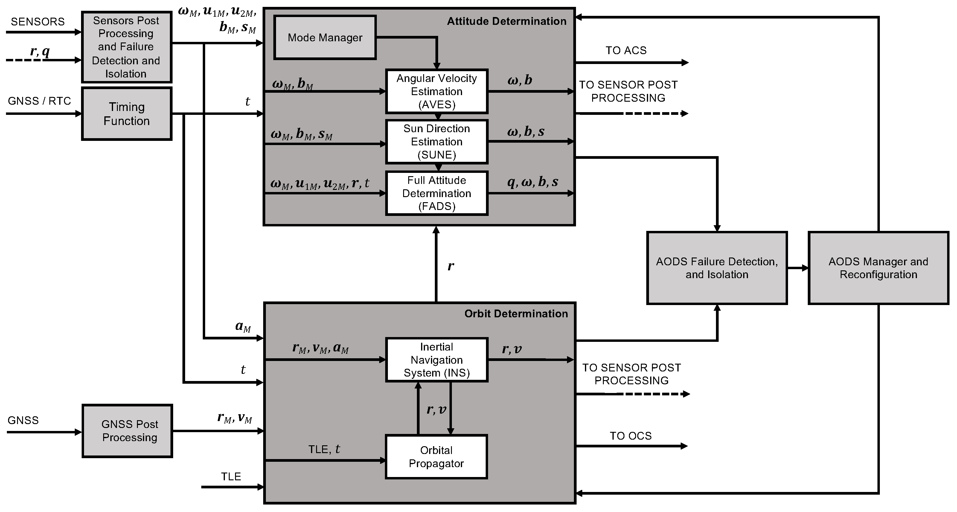
The AODS architecture is based on blocks dedicated to satisfying the estimated quantities and performance requirements according to the interfaces with the overall AOCS. The input to the AODS comes from the sensors set, while the output is sent to the following sections of the AOCS, namely, the attitude control system (ACS) and the orbital control system (OCS). If one—or both (e.g., in the case of an in-orbit demonstration (IOD) mission)—of these two control sections are not implemented, the AODS output can just be saved on-board for a sequent telemetry download to ground. For what concerns the inputs, the presented AODS architecture can be applied to any sensor suite, satisfying the imposed mission requirements. In fact, the full attitude estimation is achieved by exploiting two vector measurements. Thus, as long as two independent physical directions are measured on-board, the FADS block can estimate the attitude state. However, direct measurements of the Earth’s magnetic field, , and of the Sun direction, , shall be available to activate the direct estimation blocks (i.e., SUNE and AVES). Moreover, direct angular velocity measurements, , are needed in any operative mode, to enable dead reckoning state estimation. These assumptions are reasonable, since direct geomagnetic field measurements are needed to properly operate magnetic actuators, which are commonly used in small satellite platforms, at least as secondary actuation devices for momentum dumping. Similarly, direct Sun direction measurements are typically used to align the solar panels to the Sun during safe modes. This research is applicable to systems equipped either with star sensors, Earth sensors, Sun sensors or magnetometers but, to simplify the discussion, a common sensor configuration for small satellites is selected. From now on, the input for the AODS is assumed to be obtained from multiple Sun sensors, magnetometers and gyroscopes. The orbit determination inputs constrain the suite of needed sensors for position and velocity estimation more. In fact, a GNSS receiver is required for position and velocity measurements, and , to be combined with the output of a triaxial accelerometer, , for precise inertial navigation, even during periods when the GNSS signal is not available. In this non-nominal condition, orbital state estimation is still possible combining the inertial navigation system with on-board orbit propagations and ground-based state updates in two-line element set (TLE) format. The AODS architecture scheme is reported in Figure 1, where the primary blocks are represented, together with their main interfaces.
The sensor post processing and the GNSS post processing blocks are directly interfaced with sensors outputs. These software elements contain the drivers to receive and correctly interpret the measurements from the hardware peripheral components, the mathematical operations to scale and convert the measurements in the proper reference frame with correct dimensional units, the low-pass filters for those components without an embedded signal filtering, the measurement correction functions and the sensors failure detection and isolation (FDI) algorithms. The measurements correction functions contain all those operations needed to make the signal ready for the following estimation blocks. For instance, magnetometers are compensated for the known dipole of the magnetic actuators, accelerometers are corrected for the gravitational and for the rotation induced accelerations, Sun sensors measurements are converted into Sun direction versor and corrected for Earth’s albedo, and similar operation are performed according to the specific sensor typology. The FDI elements are based on signal processing methods and are capable of detecting and isolating loss of communication and abrupt changes in the outputs at component level. Despite the number of redundant components for each sensor typology, the measurements sent to the AODS blocks are unique for each family of sensors. Hence, the redundant measurement selection logic is also contained in the sensor post processing block.
The attitude determination section is multi-mode and, therefore, contains three distinct blocks capable of providing an estimation of certain dynamical quantities:
- The angular velocity estimation (AVES) block requires angular velocity and magnetic field measurements to provide an improved estimation of these dynamical quantities, to be used by AOCS modes dedicated to control the angular velocity of the spacecraft in body frame (e.g., detumbling, spinning rate control). The angular velocity can also be estimated by exploiting magnetic measurements, which are also needed to operate magnetic actuators;
- The Sun direction estimation (SUNE) block requires angular velocity, magnetic field measurements and Sun versor measurements to provide a good estimation of these dynamical quantities, despite the direct visibility of the Sun. In fact, in case Sun measurements are temporarily not available, the estimated Sun direction is propagated exploiting the estimation of the spacecraft angular rates. This AODS mode is intended to be used whenever simple Sun alignment is required by the operative modes of the spacecraft, without large computational costs;
- The full attitude determination system (FADS) block requires a measurement for each sensor typology. In fact, it exploits the full attitude determination system to estimate the rotation state and the angular rates of the spacecraft, the geomagnetic field vector, and the Sun direction. The attitude state is estimated in terms of quaternions, by exploiting the quaternion solutions of the Wahba’s problem [15], in the form of the quaternion estimator (QUEST) algorithm [16,17]. The angular velocity and the magnetic field measurements are respectively calibrated on-board by means of a complementary filter [13] and of an iterative nonlinear least squares filter [18,19]. The FADS block can be executed as long two independent versor measurements are available, together with a measurement for the angular rates and for the position of the spacecraft. The latter is needed to feed the environment models to solve the attitude problem with respect to an inertial reference frame. The magnetic field and Sun direction estimates in body frame are obtained from the processed measurements, if they are available, or by rotating the environment models data from the inertial reference frame.
The different attitude determination modes are activated from the output of an embedded mode manager function, which is activated according to the commands coming from the platform operations, to be combined with the feedback commands of the AODS manager. In fact, in the case of AODS detected failures, the recovery reconfiguration can override the primary commands from the platform, to operate the system in fault tolerant mode, in agreement with the non-nominal condition. In the eventuality that the AODS reconfiguration is not compatible with the platform operations, a safe mode transition is commanded to the spacecraft mode and vehicle management system.
The orbit determination section can be operated in two modes that are identical in terms of block outputs, but are differentiated at measurement level, according to position and velocity sources. In fact, orbit determination is intrinsically working in single mode with two alternative measurement sections:
- Inertial navigation system with GNSS and accelerometer measurements, which requires the complete availability of all the orbit determination sensors. In this mode, the gravitationally corrected measurements of the IMU are combined in a Kalman filter to improve position and velocity estimates, and to estimate the accelerometer and gravitational model errors;
- Inertial navigation system with orbital propagator and accelerometer measurements requires a valid estimate for position and velocity, either from the previous step of the orbit determination algorithm, or from ground knowledge of the current orbital TLE set. The Kalman filter is modified in terms of measurement models and covariance properties. Moreover, the estimation of accelerometers errors is not updated in this mode, and the orbital propagator outputs are combined with constant calibration data for the IMU measurements.
The two orbit determination modes are not connected with a mode manager, being the availability of GNSS data the only element to select the proper INS mode. Thus, the GNSS post processing and failure detection block is used to generate a command to activate one operational mode or the other. The proposed INS implementation allows to estimate the errors on position and velocity, with the error dynamics inside the Kalman filter that is capable to reduce the divergence rate of the orbit determination error when the GNSS signal is not available. In the case the accelerometers are failed, position and velocity data can be directly retrieved from GNSS measurements. Note that the orbit determination block is closely coupled with the FADS block, being the position of the spacecraft needed by the FADS function, as explained above. Moreover, the full attitude state is needed for the inertial navigation with MEMS strap-down sensors, and it is used in the accelerometers’ post processing block.
The system level failure detection and isolation block is combined with the reconfiguration logics in the AODS manager to enable recovery capabilities in the eventuality of non-nominal scenarios. These blocks gather all the available status information from the AODS, from the commanded nominal AODS mode, to the health conditions of the sensors, up to the error status of attitude and orbit determination functions. If a non-compatible status is evident by analyzing the combination of those parameters, the failure detection monitor rises an error flag. Then, dedicated isolation algorithms are activated to confirm the failure and analyze the set of potential redundant configurations. In particular, they check for previous failures, they try to reboot the failed elements, and they explore the availability of redundant components or functions. From the output of these algorithms, the AODS manager block reconfigures the system in accordance with the current operative mode of the platform. For instance, it commands the activation of redundant sensors, or the execution of alternative estimation algorithms, to guarantee the required outputs from the AODS block. If this is not possible, a platform safe mode is requested, and an AODS mode transition towards a compatible mode is commanded.
The timing function block is a fundamental element in the proposed AODS architecture. This component is required to provide accurate timing to execute the AODS—and the AOCS—functions. Absolute and relative timing are required, the former guaranteed by the GNSS signal, the latter preserved by a real time clock (RTC) embedded in the on-board processing units. The fault tolerant properties are also preserved in this block, being a failure in the GNSS mitigated by a close-loop integration of the absolute timing with the relative one. Furthermore, in the case where the GNSS signal is lost, absolute timing updates from the ground can be guaranteed.
The proposed AODS architecture has been outlined for implementation in typical small satellite hardware. In particular, the limits in the available computing performances are applied as a strong constraint for the AODS modes design, considering their integration with the entire platform software and the computational burden of the whole spacecraft system modes. In particular, the present AODS has been intended for 10 Hz operations in a 32-bit RISC microcontroller unit running at 64 MHz, with 32 MB of SDRAM.
3. Sensor Post Processing
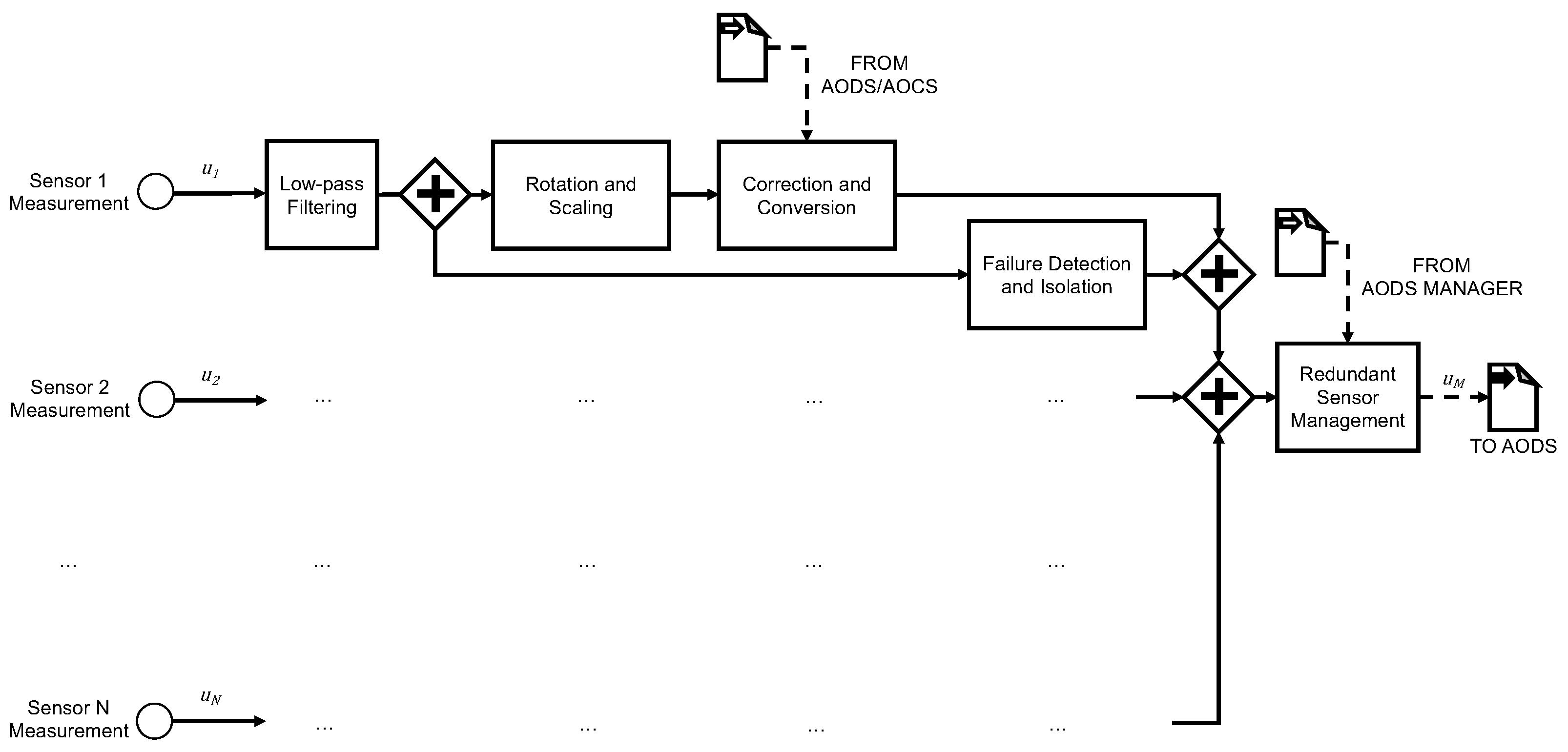
Sensor post processing blocks are required to gather the sensor signals, interpret them according to structured data formats and convert the signals into a value to be used for the following estimation operations. This paper does not enter the details behind the communication interfaces with the sensors and, thus, the input to the post processing blocks is assumed to be the raw, uncalibrated, unscaled numerical value, representing the sensor measurement according to the sensor’s datasheet. The specific post processing operations depend from the sensor type, but they can be resumed by the following steps, also graphically represented in Figure 2:
- Low-pass filtering, if not performed by the sensor unit;
- Reference frame rotation and unit dimension scaling;
- Measurement correction and conversion;
- Failure detection and isolation at component level;
- Redundant sensor management.
Precisely, the filtered sensor signals are processed to obtain the desired measurements and they are used to detect the sensor faults. These two processes run in parallel as shown in Figure 2, and their outputs are combined, together with those of the other redundant components, to be used by the redundant sensor manager. In fact, the measurements sent to the AODS section are eventually processed by the redundant sensor manager, which select, among the available sensor data, the best one to be used for attitude and orbit estimation. Hence, for any measured physical quantity, the AODS uses a single value at a time as:
where N is the number of redundant sensors. The best measurement is selected by analyzing the time variance of the signals, as will be described in the next sections discussing the details of each sensor post processing block.
3.1. Filtering, Rotation and Scaling
The low-pass filtering operations are performed only on those sensors without an embedded low-pass filter. A fourth-order Butterworth filter is used, with a cut-off frequency compatible with the sampling time and the signal dynamics. The rotation operations convert the sensor reference frame into the spacecraft body frame, and the scaling is needed to convert the sensor output in international system (SI) units. The definition of the exact sensor reference frame requires accurate measurement operations at ground testing level.
3.2. Measurement Correction and Conversion
The measurement correction and conversion blocks strongly depend on the specific sensor typology to which it is associated. In general, this function is needed to correct the signal from spurious phenomena not directly belonging to the AODS. This process shall not be confused with the on-board calibration of the sensor, which is an operation that is used to estimate an unknown quantity to improve the attitude or orbit determination performance. The measurement correction function uses a model of the spurious effect to be corrected to prepare the sensor readings for correct usage in the AODS. Some sensor typologies also require dedicated conversion functions to convert the raw sensor signal into a useful quantity for the following estimation functions. For example, this is the case for Sun sensors based on photodiodes, Earth sensors based on thermopiles, or other typologies of basic sensing instruments that are very common on small spacecraft platforms.
3.2.1. Accelerometer Correction
Accelerometers for small satellites are based on strap-down inertial sensor technology [20], which requires to have an estimation of the attitude of the body to which the sensor is rigidly attached in order to generate a coordinate transformation that operates on the accelerometer measurements, giving an acceleration resolved into inertial axes. Moreover, accelerometers are not capable to measure gravitational accelerations, and they are typically not placed in the center of mass of the system. Thus, accelerometer measurements shall be corrected for the gravity field and for the accelerations due to the spacecraft rotation. Then, they shall be rotated from the body to the inertial reference frame. The correction to the acceleration measured from the i-th accelerometer results in:
where is the rotation matrix from the body frame, B, and the inertial frame, I, is the body angular rates, is the position vector of the i-th accelerometer in body reference frame, and the gravitational acceleration, function of the spacecraft position, . The apexes or are used to indicate the reference frame in which a physical quantity is expressed or measured. To avoid a cumbersome notation, they are indicated only in those situations where confusion may arise. The tilde over the symbol indicates the physical quantity before correction and conversion operations.
The gravity field acceleration is computed from a model of the gravitational field of the Earth, knowing the position of the spacecraft. To simplify the on-board computation, and to avoid any dependence from the Earth fixed reference frame in Equation (2), the gravity acceleration model is implemented up to term:
where is the standard gravitational parameter of the Earth, and the acceleration term, , is expressed as in classical orbital mechanics books [21].
3.2.2. Magnetometer Correction
The magnetometer measurements shall be corrected for the known magnetic interactions with the spacecraft components. In fact, in small satellite platforms, the magnetometers are typically very close to the spacecraft electronics, and not placed far away from other system components, such as on the tip of a deployable boom. For these reasons, internal magnetic disturbances affect magnetometers measurements. In particular, the magnetic torquers have a non-negligible effect that may produce large errors on the following attitude estimation. Thus, the correction to the i-th magnetic field measurement is applied as:
where is the magnetic dipole commanded from the ACS to the magnetic torquers, and is the coupling matrix between the i-th magnetometer and the magnetic torquers, which depends on the distance of the sensor from the actuators and on the mean permeability of the body materials. can be estimated on the ground with electromagnetic testing activities, and it is typically a function of the inverse of the cube of the relative distances between magnetometers and magnetic torquers.
3.2.3. Sun Sensor Correction and Conversion
Sun sensors’ correction and conversion operations strongly depend on the sensor technology and implementation. Generally, Sun sensors for small satellites are composed by single or multiple photodiodes generating electrical currents proportional to the cosine of the Sun angle with respect to the sensor normal, , as:
where is the maximum current produced when the light source is directly above the cell, and it is measured by ground testing. The specific assembly of the photodiodes within the sensor, as well as the way in which the electrical current is measured (e.g., absolute current measurements of each cell, differential measurements between adjacent cells or rows of cells, …), determine the conversion function to compute the Sun direction from the electrical currents:
where S is the number of photodiodes used in the specific Sun sensor assembly. Usually, fine Sun sensors are composed of a matrix of several photodiodes capable to accurately detect Sun direction with differential current sensing, and specific optical or geometrical assemblies. On the contrary, common coarse Sun sensors are simple photodiode cells installed on the spacecraft external faces. In this case, the Sun direction is simply obtained combining the measurements coming from at least three independent faces normal to distinct directions. For example, assuming there are S identical photodiodes on each of the six faces of a cubesat, the Sun direction can be computed from Equation (5) as:
where n denotes the normal direction versor of each face in body reference, . Then,
Despite the specific conversion function, the post processing block eventually gets to a measured Sun direction for any i-th sensor. These measurements shall be corrected for the Earth’s albedo spurious signal, which may affect sensor accuracy by more than 100%. To perform this operation, the Earth’s direction in body frame shall be computed from the orbit determination output, and an albedo model shall be implemented. Hence, the Earth’s angle with respect to the sensor normal is:
At this point, Equation (5) is applied to estimate the current term produced by the Earth’s albedo as:
where is a coefficient scaling the output current according to the lower intensity of Earth’s radiation, and to the different photodiode’s response to the light’s spectrum of albedo. Note that, for a generic Sun sensor, the current generated by the Earth’s albedo can be computed inverting the specific conversion function:
In any case, the albedo correction is applied by computing Equation (6) or Equation (7) with a current offset for the albedo estimated contribution:
The albedo correction function shall consider the proper albedo intensity in the operational orbit of the spacecraft and, more importantly, it shall apply the albedo correction only when the Earth is illuminated. Thus, this correction operation shall detect, from the intensity level of all the Sun sensors on the spacecraft, whether the system is currently in eclipse or not. Furthermore, specific calibration coefficients for Equation (11) shall be computed during ground testing to account for the finite dimension of the Earth, which is not a point light source at infinite distance.
Solar panels’ power signals can be processed by dedicated post processing functions, using Equation (5), in order to exploit the solar arrays as a further set of coarse Sun sensors. This option can be exploited in the survival modes of the spacecraft.
3.2.4. GNSS Conversion
GNSS conversion is required to convert the positioning data from the Earth’s fixed reference frame to the inertial reference frame, used in the orbit determination section. Specifically, the performed conversion is from the Earth-Centered Earth-Fixed (ECEF) reference frame, as defined by International Astronomical Union, to the Earth-Centered Inertial (ECI) J2000 reference frame. The transformation between the ECEF and the ECI is performed through a series of four rotations that are known as Earth orientation models, which are parametrized by the Earth Observation Parameters (EOP) data. The GNSS conversion is performed according to the IAU-76/FK5 reduction approach, applying the corrections for the EOP [21]. The GNSS conversion function also extracts the timing from the GNSS data to synchronize the frame conversion operations. So, the GNSS conversion function is strongly dependent from time accuracy, and for this reason this post processing block is paced by exploiting the pulse per second (PPS) signal coming from the GNSS receiver. The GNSS conversion block also converts the positioning data in other formats, such as latitude, longitude, ellipsoidal height data in the ECEF frame, and NMEA standards. These formats can be conveniently exploited in standardized telemetry data.
The gyroscopes do not require any correction and conversion function, and the only post processing preliminary operations are those for reference frame rotation and unit dimensions’ scaling. Note that common MEMS gyroscopes for aerospace applications are also typically equipped with internal low-pass filters.
3.3. Component Level Failure Detection and Isolation
Failure detection and isolation functions at component level operate on sensor signals after low-pass filtering. Thus, the failure detection is performed on the raw filtered sensor measurements, and it is based on statistical analysis on the incoming signal. These functions operate on the low-pass filtered data in order to have a uniform behavior among sensors with and without embedded low-pass filtering.
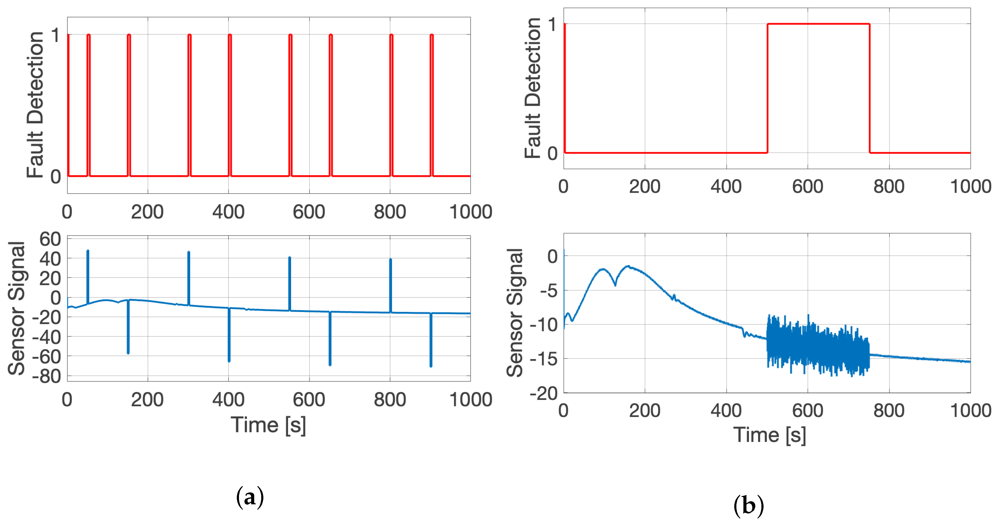
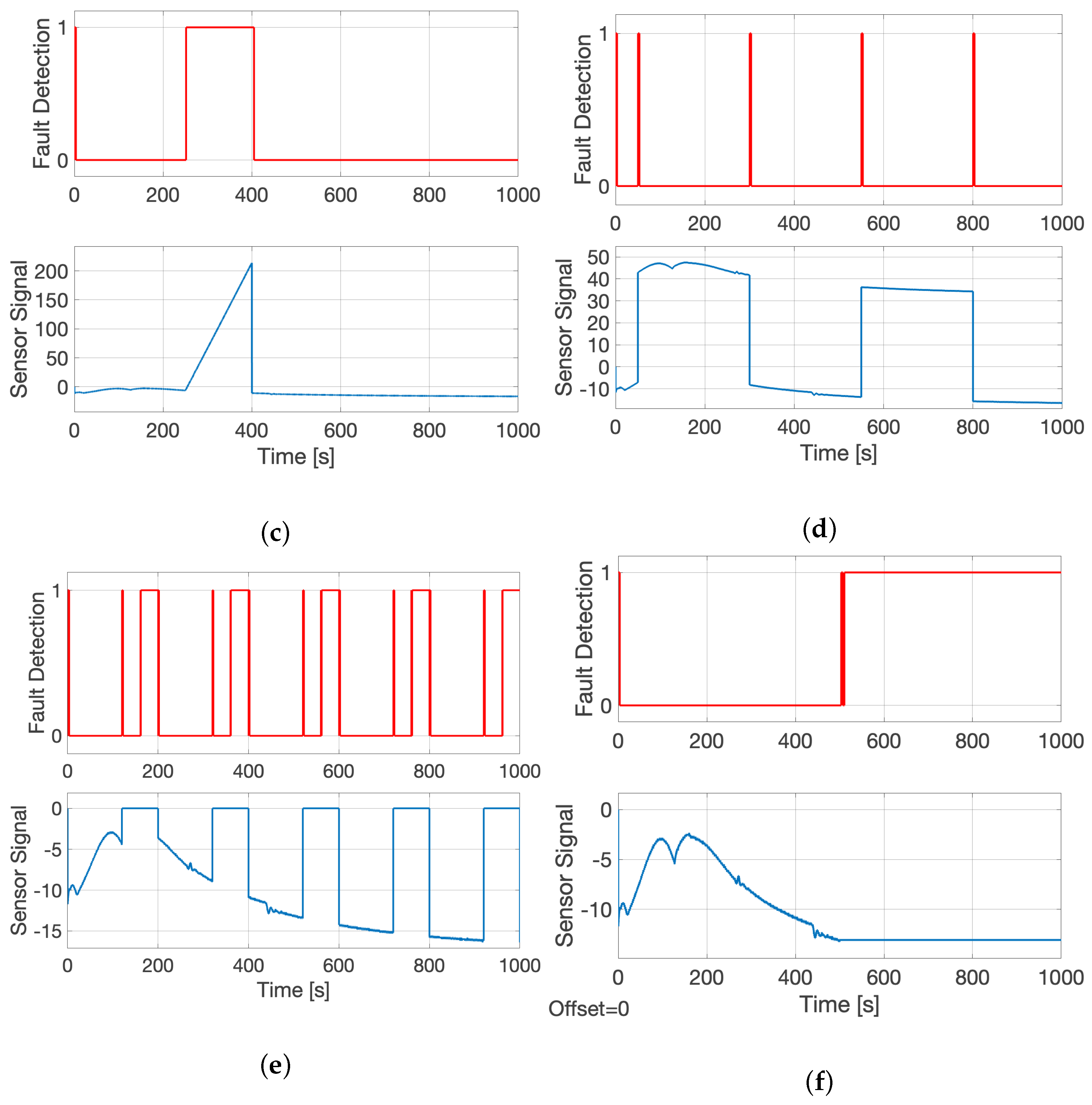
The statistical algorithm is designed and calibrated in order to detect the most common typologies of sensor faults: spike faults, erratic faults, drift faults, hardover/bias faults, data loss faults and stuck faults [22]. These faults can be defined as follows:
- Spike fault: spikes are observed in the output of the sensor;
- Erratic fault: noise of the sensor output significantly increases above the usual value;
- Drift fault: the output of the sensor keeps increasing or decreasing from nominal state;
- Hardover/bias fault: the output of the sensor has a sudden increase or decrease with respect to the nominal state;
- Data loss fault: the output of the sensor has time gaps when no data is available;
- Stuck fault: the sensor’s output gets stuck at a fixed value.
The complexity in detecting these faults is related to the dynamical evolution of the nominal sensor signals along a generic attitude state. In fact, in general, none of the sensor outputs has a steady state constant value, and the detection algorithms should be capable of detecting a variation that is not compatible with a feasible dynamical state of the spacecraft. In fact, spacecraft nominal rotations are bounded below maximum angular rates. Similarly, the angular accelerations are very small and are limited by the maximum actuator torques. Thus, there exists a maximum feasible time variation of the sensor signal that can be used to distinguish realistic measurements from faulty ones. The possibility of marking real measurements as faulty ones (e.g., the spacecraft is experiencing a non-nominal attitude dynamics) is minimized with the application of system level failure detection functions, which are designed to compare different measurements and to detect dangerous conditions for the entire system. However, the design approach is conservative. Then, it is preferred to detect false failures, rather than having failure propagation in the AODS.
The failure detection algorithms are based on the running variance and running mean of the sensor signals. The running variances are used to detect the common sensor faults described above, while the running mean is applied to detect the presence of a valid sensor output. For this purpose, the sensor driver sets the sensor measurements equal to 0 if the sensor data are not received or received as corrupted packets. Running variance and running mean are computed on the last S samples of the j-th sensor scalar measurement as:
where is the time associated with the S-th sample. If a sensor measures a vectorial quantity with multiple components, the running mean and variance are computed for each component of the vector:
A good sampling interval is defined in the range of S from 10 to 100 samples for AODS running at 1 to 10 Hz.
A sensor is said to be non-faulty if the running mean of the running variance is greater than zero and smaller than a given threshold. If the sensor measurement has multiple vector components, the minimum running mean of the running variance components shall be greater than zero, and the maximum component shall be below the given threshold. That is, a sensor is properly working if:
If these conditions are not respected, the failure is detected. If the minimum component is equal to zero, the sensor has a stuck fault. If the maximum component is above the threshold, the other faults can be present. The running mean of the variance is used to smooth the failure detection response, and neglect confined errors in the signal. The following isolation functions are designed to understand the specific fault typology. For example, a high variance with fluctuations can indicate an erratic fault, short and repeated peaks in the variance can indicate spike faults, a single short peak in the variance can indicate a hardover fault. Drift faults are more difficult to be detected unless the drift is very fast. In this case, the variance has a significant constant increase with respect to nominal values. The variance threshold, , is specific for any sensor and it is calibrated by ground testing. Moreover, its value can be updated while the spacecraft is in orbit to better tune the sensitivity level of this failure detection logic. The selection of the value is crucial to distinguish between feasible variations in the signal due to attitude motion, and variations due to faults.
A sensor is said to be operative if the square of the running mean—or the square of the minimum running mean component of a vectorial signal—is greater than zero. Thus, a sensor sends valid outputs if:
If this condition is not respected for a prolonged time, the sensor is completely off. On the contrary, if the condition is not respected for short and close intervals of time, a data loss fault may be present.
A failure is detected in the sensor if either Equation (16) or Equation (17) is not respected. In this case, specific isolation functions are activated to avoid failure propagation and understand the fault typology. Some failure detection examples are shown in Figure 3. At first, if a failure is detected in a sensor, the redundant component manager is commanded to use the redundant sensors, and the outputs of the failed component are blocked. The isolation function continues to sample the faulty unit for few seconds in order to better classify the failure (e.g, distinguish between a spike and a hardover failure) for the following analyses on ground. Then, a reboot of the sensor is executed, followed by a health monitoring sampling. If the sensor shortly repeats the fault, the component is switched off and labelled as non-operative. On the contrary, the component is sent back to the AODS sampling, but if another failure is detected within a certain time interval (e.g., in the order of few minutes), the component is finally removed from the AODS loop. In any case, ground commands can override any failure detection and isolation on-board decision.
3.4. Redundant Component Management
The redundant components are managed by a dedicated function that elaborates inputs coming from the AODS manager and reconfiguration section, from the failure and isolation functions, and from the corrected sensor signals.
Sensors with detected failures are automatically excluded from the following AODS loop. In fact, as long as isolation functions—or ground commands—do not confirm the correct re-initialization of the component, the failed sensor signal is blocked from further processing. This is accomplished with a failure flag issued by the FDI block and associated with the faulty component measurements. If no sensor of a given typology is still available after a failure detection and isolation event at component level, the system level FDI detects it, and the AODS manager reconfigures the system to satisfy the current operative mode requests or, if this is not possible, it selects a proper safe mode or it commands a fatal ADCS error to the platform.
AODS manager commands are interpreted to provide the AODS with measurement data, as required by the current nominal configuration. For instance, if the angular velocity estimation block is the active attitude determination function, the redundant sensor manager provides the AODS with angular velocity and magnetic field measurements. Similarly, if a reconfiguration is commanded, the sensor manager selects an alternative set of sensors to guarantee the proper operations in the AODS block. The combined action of redundant sensor manager and AODS manager is designed to always select the bast available sensors and modes to support the current operative mode.
When the information coming from the FDI and the AODS manager blocks leaves more than one redundant sensor available, the redundancies are managed by exploiting the running variance computed in the previous sensor post processing section. In fact, the variance information of a given signal is directly dependent from the variance of the measured quantity and the variance added by the measurement operations. Since the measured quantity is the same for all the redundant sensors of a given typology, two redundant sensors have a different variance only because of distinct measurement errors. In general, a higher variance is associated to larger stochastic errors in the measurements. Hence, the signal to be used in the AODS section is selected as:
An example output for the redundant component manager is shown in Figure 4.
This selection is performed whenever there are at least two redundant sensors of comparable quality (e.g., bias, random walk errors, …). However, when the quality of the sensors is much different, as verified during ground characterization, the component selection is only driven by sensor data availability. For instance, coarse Sun sensors are only used if fine Sun sensors measurements are not available, or if required by the AODS manager. In these cases, it is a good practice to set the failure detection threshold of the accurate sensors below the typical variance level of the coarse ones.
Note that very coarse sensors can be kept switched off during nominal operations, and they can only be activated if required by the redundant component manager.
4. Attitude Determination
Attitude determination section’s algorithms are dependent from the specific mode. Angular velocity and Sun direction estimation functions directly take the sensor measurements and apply a low-pass filter to smooth the output of the AODS. These blocks are not characterized by specific estimation methods, but they are capable to provide the same fault tolerant performance of the whole AODS. In fact, these blocks can handle the input from main and redundant sensors, and they can propagate the dynamics exploiting angular rates measurements, in case of direct sensor loss.
Full attitude determination is more delicate and guarantees a full attitude estimation, even after multiple faults. With the assumption of exploiting Sun and magnetic field measurements, the inputs to FADS are:
with the addition of the position vector estimate from the ODS, , and the current time, t. The latter quantities are used in the on-board ephemerides of the Sun, and in the IGRF model of the Earth’s magnetic field, to retrieve the directions of magnetic field and Sun in the inertial reference frame: and . The algorithms of this section provide error estimation for on-board sensor calibration, to improve the overall determination performance. Thus, the measured quantities are calibrated as:
where and are, respectively, the estimated bias vectors for gyroscope and magnetometer, and is the fully populated matrix of scale factors and non-orthogonality magnetometer errors. The gyroscope measures are unbiased thanks to the angular velocity bias estimation performed with a complementary filter [13]. The magnetometer measures are unbiased as well thanks to a sequential centered iterative algorithm [19]. Note that Sun direction measurements are not further calibrated after the Albedo correction in the sensor post processing section.
The static attitude determination logic uses the calibrated measurements to statistically solve the Wahba’s problem. Magnetometer and Sun sensors are weighted in the QUEST implementation according to their quality, as measured with the mean of the variance computed in the sensor post processing section:
where and are non-negative weights respecting . The outcome of the statistical attitude determination is the estimation of the spacecraft’s orientation, in terms of quaternion, , and angular velocity, . The bias estimation algorithms use the output of the static attitude determination, combined with angular rates measurements, to obtain the calibration coefficients described before. Whenever enough information from the sensors is not available, a dead-reckoning estimation is initialized from the last valid attitude state and the dynamics is propagated with the unbiased output of the gyroscopes. The calibration coefficients are not updated during the propagation periods.
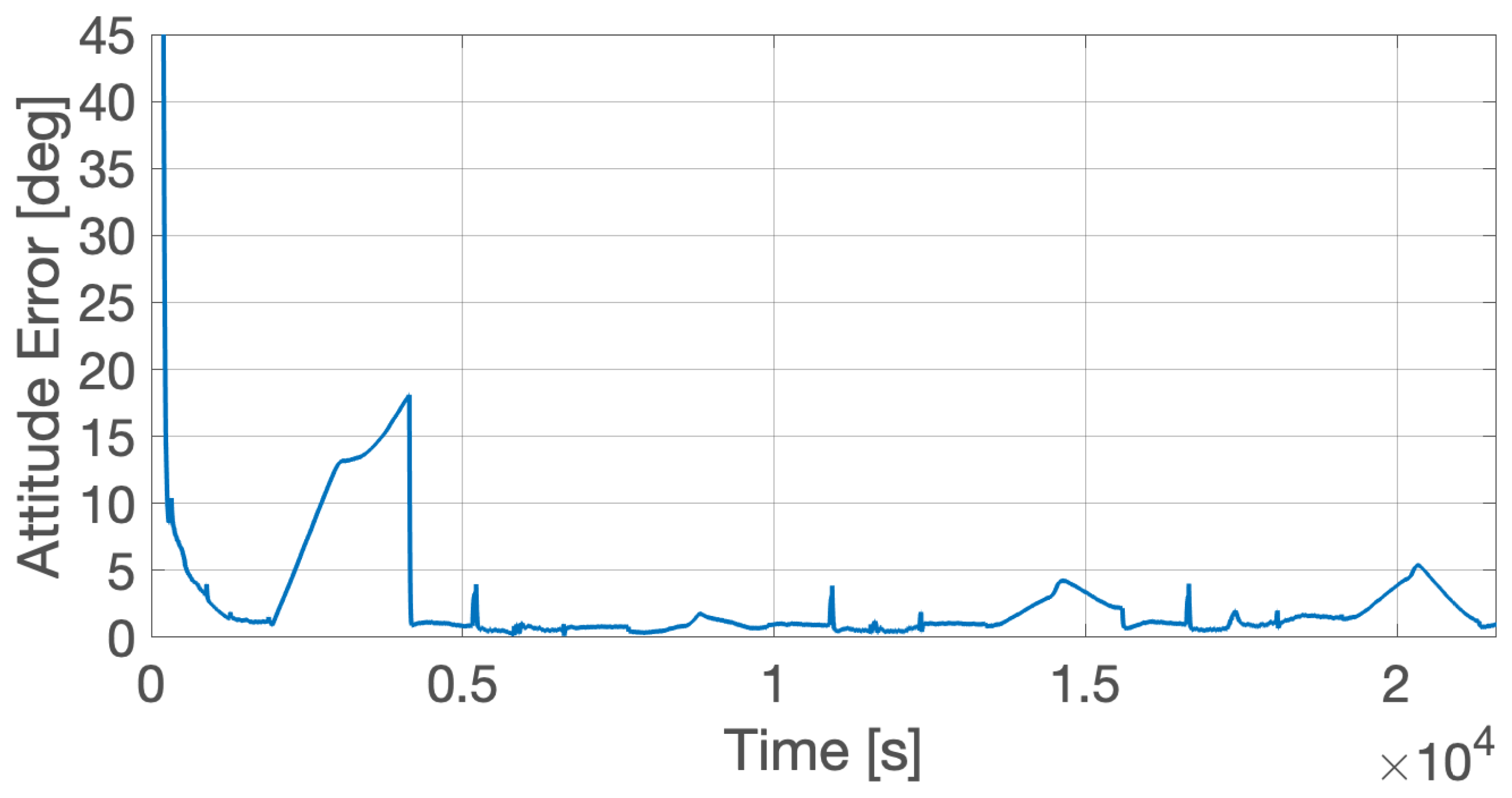
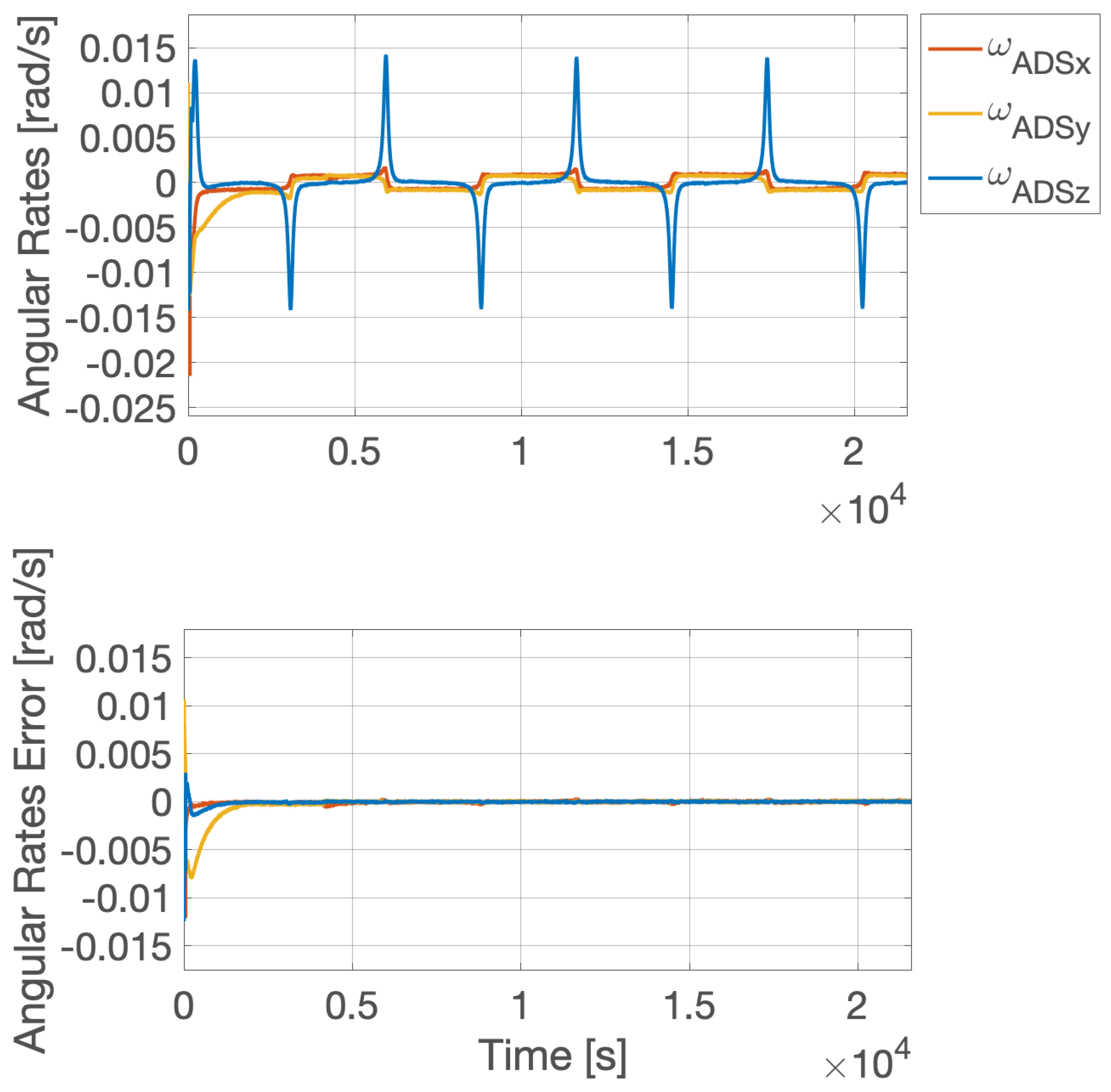
Figure 5 shows an example AODS output in Earth pointing mode, initialized from unknown initial attitude state (e.g., lost in space condition). The results are obtained from a verification campaign at MIL level of the proposed AODS. The figure reports the three-axis error angle between the estimated quaternion and the model one, used as reality reference. The determination performance is better than ∼ deg, whenever the gyroscope bias is correctly estimated. In fact, the large error drift between s and s is due to the first attitude propagation in eclipse, which exploits a preliminary estimation of the gyroscope’s bias. The following dead-reckoning periods during eclipses (i.e., 9000 s, 15,000 s and 20,000 s) introduce a propagation error limited to 2 deg–3 deg along a ∼ min eclipse. The small ∼ deg peaks in the attitude error graph are due to the loss of the fine Sun sensors’ measurements, immediately replaced with the measurements of the coarse sensors. All the sensors used in the proposed analyses have a typical performance for small satellite platforms. Figure 6 shows the estimated angular rates, and the errors with respect to the reality reference for the same simulation scenario. From this figure, ia non-precise bias estimation before s can be noted, which influences the first dead-reckoning period.
5. Orbit Determination
The orbit determination algorithm is based on an inertial navigation system with GNSS sensors and accelerometers integration. This block provides a full orbital state estimate in terms of inertial position and velocity, using positioning and acceleration measurements:
The accelerometer bias term estimate is continuously updated to calibrate the accelerometer measurements:
The accelerometer measurements are unbiased thanks to the bias estimation performed with an extended Kalman filter (EKF) [23].
The ODS algorithm is formulated in a closed-loop loosely coupled architecture. Accelerometer readings are used to propagate the inertial state vector generating the INS preliminary estimate, while GPS measurements are compared with the INS estimate to generate a measurement error signal. The measurement error signal is fed to the extended Kalman filter, which outputs an updated estimate of the position and velocity error, as well as the bias term estimate. Eventually, the output of the EKF is used to correct the INS preliminary estimate, whereas the bias term is fed back to the integration block of the accelerometer measurements. In the case the GNSS is experiencing an outage period or a fault, an on-bord orbit propagator is used as synthetic measurement element for the INS input. The orbit propagator includes atmospheric drag and perturbation effects and it performs dead-reckoning of the orbital state as soon the GNSS measurements are lost. In this case, the EKF exploits a different measurement model and covariance matrix with respect to the nominal mode with GNSS and accelerometer coupling. Obviously, the approximate orbital model introduces propagation errors, and an inherent position drift cannot be avoided. However, the coupling with the EKF helps in accounting for the orbital error dynamics, and it determines a slower divergence rate with respect to a pure on-board orbital propagation including the same perturbation terms. In this condition, the orbit determination and propagation can be periodically updated from ground with upload of the spacecraft position in the form of TLE set.
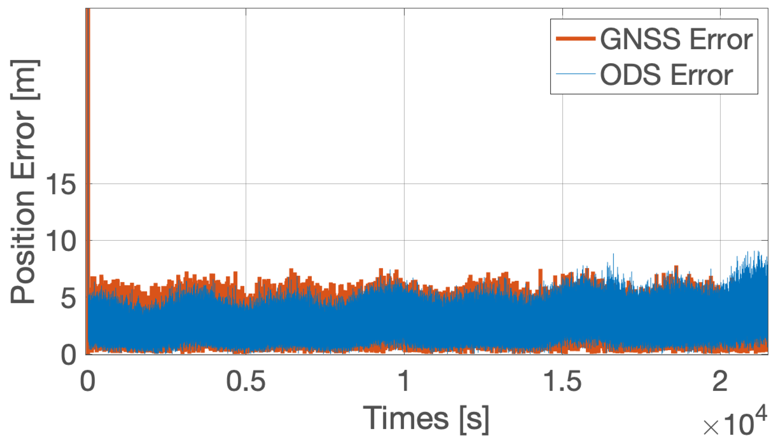
Figure 7 reports an example ODS output for a low-Earth orbiting satellite. The results are obtained from a verification campaign at MIL level of the proposed AODS. The figure reports the three-axis position error between the estimated position and the model one. The accuracy of the position estimation is around 5 m, with a slightly better performance with respect to the raw GNSS measurements. However, the main purpose of the proposed architecture is to provide a fault tolerant orbit determination system, whose fault tolerance performance will be discussed in the following.
6. System Level Failure Detection
System level failure detection functions are dedicated in detecting failures in the AODS by combining all the outputs from attitude and orbit determination blocks. These functions detect:
- Missing measurement for a desired physical quantity, which is associated to the lack of sensors for a given typology;
- Excessive angular rates of the spacecraft, which is associated to an unexpected tumbling dynamical status;
- Non valid or corrupted attitude determination data;
- Non valid or corrupted orbit determination data;
- Errors in attitude and orbit determination mode management;
- Non correct attitude estimation.
For any of these errors, the AODS manger and reconfiguration block receives a specific output of the failure detection and isolation at system level and commands a dedicated counter measurement. Most of the listed faults require a safe mode activation, or even an AODS re-boot. However, certain specific conditions may be solved by commanding a system reconfiguration.
Tumbling failure is detected by comparing all the available angular rate measurements on-board. Both those from raw sensor measurements, and those from estimation functions. Moreover, magnetic field time variations are also used to have a rough estimation of the on-board angular rates [24]. All these data proportional to the angular rates are compared with respect to a tumbling detection threshold. If more than one measurement source is above the selected threshold, then the excessive angular rates failure is detected.
Non correct attitude estimation failure is detected by comparing the output of the AODS with respect to the power measurements coming from the electric power subsystem (EPS). The estimation of the Sun direction in body reference frame is used to compute the electric current generated from the i-th solar array by exploiting Equation (5) as:
where is the normal direction with respect to each solar panel. Then, these estimated current values are combined and processed to obtain the same data available from the electric power subsystem telemetry. If the difference between the estimated power signal and the measured one is different by more than a certain threshold percentage, the failure is detected. Good failure detection results, without significant false triggers, have been obtained with a threshold difference in the order of 30%.
7. System Reconfiguration and Recalibration
The failure of the AODS, as detected by the FDI at the system level, are managed by the AODS manager, which tries to recover the failures by commanding system reconfiguration and recalibration. System reconfiguration alternatives implemented in the proposed AODS are:
- Switch between fine and coarse Sun sensors for nominal attitude estimation;
- Switch between coarse Sun sensors and solar array data to retrieve Sun direction measurements;
- Switch between gyroscope angular rates measurements and magnetometer angular rates estimation [24];
- Switch between alternative typologies of sensors, if available, to measure two independent directions;
- Switch on redundant low accuracy sensors to supply the needed measurements;
- Change the AODS mode and command, if needed, an ADCS safe mode towards a simpler and more robust operative mode.
In this last condition, for example, a faulty FADS mode can be substituted by a simpler Sun estimation, achieved with the SUNE mode. If the nominal platform mode was a Sun pointing, then no safe mode transition is required. Alternatively, if the nominal platform mode was a three-axis stabilized pointing, a Sun pointing safe mode shall be commanded. In the worst case scenario, the angular rate estimation performed in AVES mode is very robust to support angular rate control, to achieve at least a spin attitude stabilization. The AVES mode is robust because it can be fully operated with both gyroscopes and magnetometers only. Hence, if this AODS mode is not available, the entire subsystem is probably lost. Table 1 reports an example reconfiguration table that can be used to manage system level failures. Note how the AODS manager and reconfiguration block shall be interfaced with the mission and vehicle manager, since a failure in the sensors can drive a reconfiguration at vehicle level. For example, from the reconfiguration table for detumbling mode, magnetic actuators cannot be used in the case magnetic field measurements are not available on-board. Similarly, a coupling between ADS and ODS is evident. In fact, a failure of the ODS block, determining the loss of the position estimate, induces a transition from FADS mode to another ADS mode, such as the SUNE.
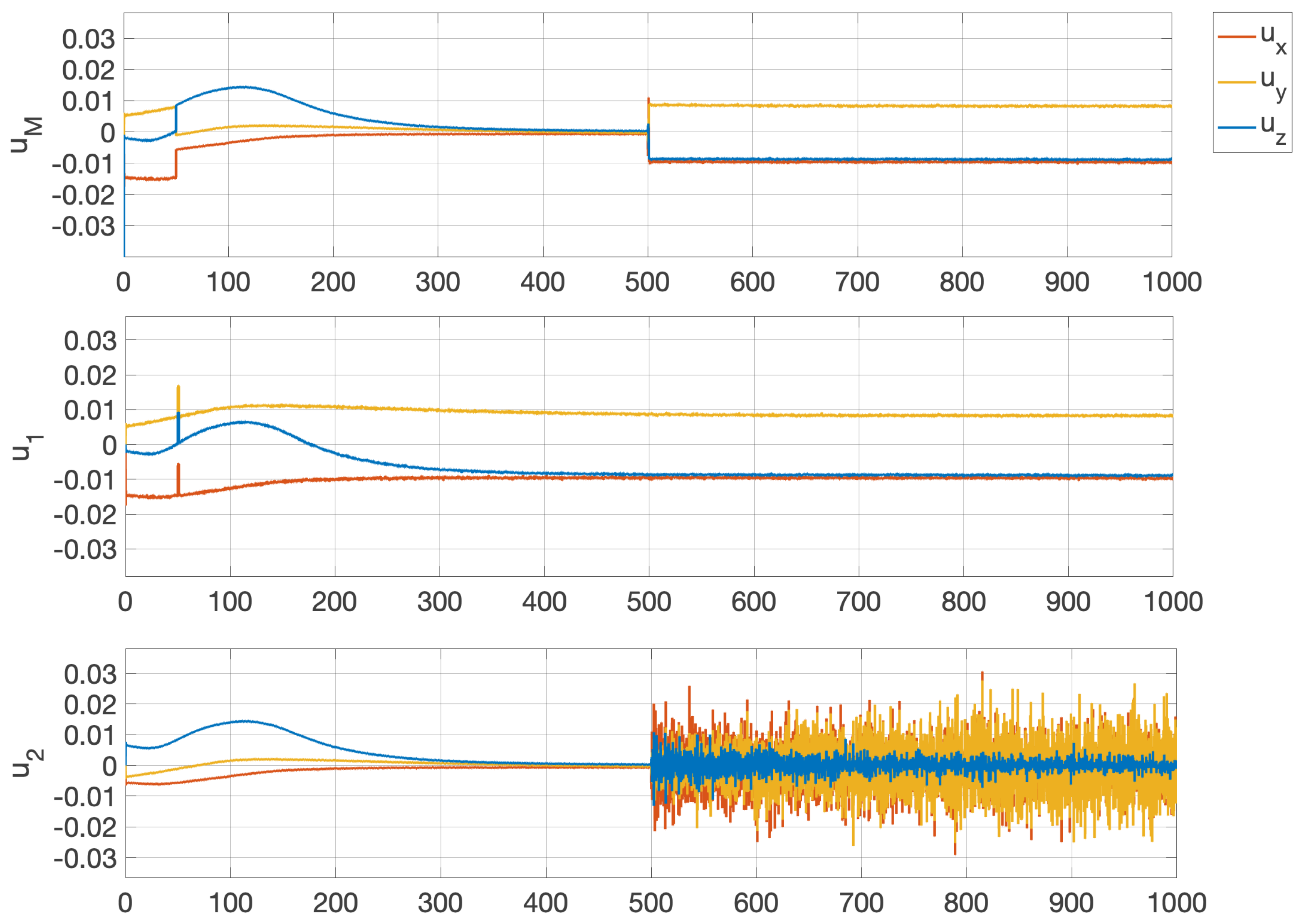
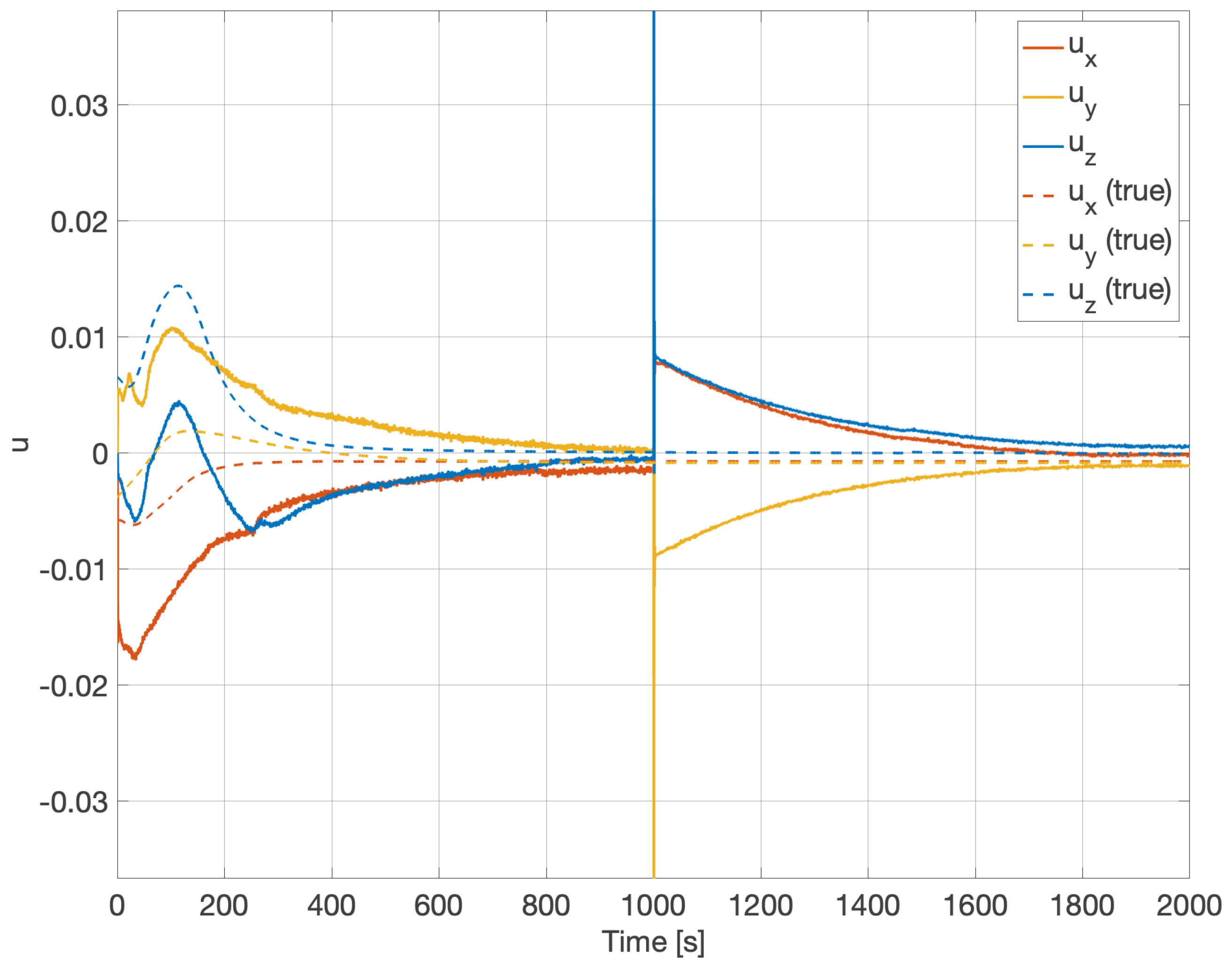
Whenever the system is reconfigured, the last calibration data involved in the reconfiguration shall be substituted. For instance, estimated gyro bias, albedo correction terms or estimated magnetometers errors shall be re-initialized selecting the initial conditions for the new calibration terms, which have been estimated with ground testing, or imposing zero initial conditions. This operation is performed by the AODS manager, and there is a settling time before design performances are re-established. Thus, the mission manager shall consider the needed transient time in order to properly operate the system. Figure 8 reports a simulation with a recalibration event. It shall be noticed how the switch to a redundant sensor with large measurement offset bias, at s, is compensated with a system recalibration completed in less than min. Similarly, the initial calibration from unknown bias values at s is completed just before the FDIR action and the switch to the redundant component.
8. Fault Tolerance Performances
The proposed fault tolerant AODS for small satellite platforms shall also be assessed in terms of fault tolerance performance. In fact, the AODS architecture guarantees the system operations even in the case of multiple faults have occurred. Obviously, the estimation performances are degraded, but the system is still capable of providing a state estimation. Redundant sensor management acts immediately with a switch between redundant components, stopping the failure from propagating further into the determination system. Thus, if the redundant components are equivalent to the primary ones, no change is evident in the output. However, if the failure involves all the sensors of the same typology, the system reconfiguration and recalibration need some time to adapt to the new operative condition.
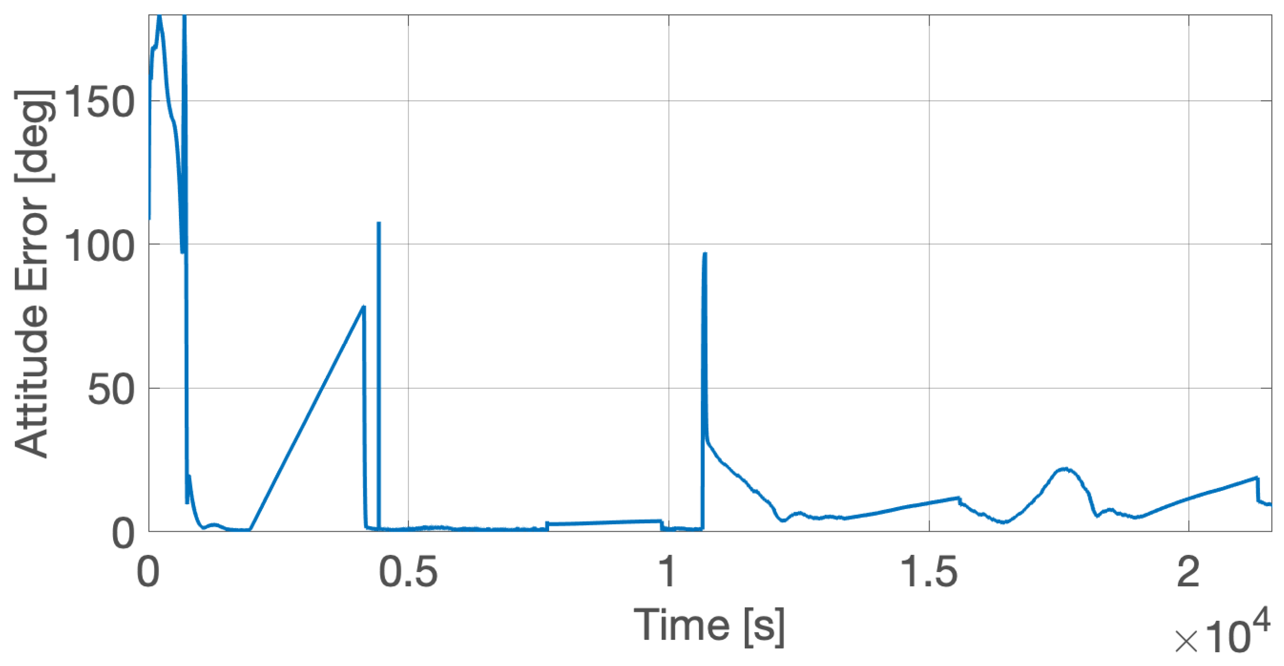
Figure 9 shows a MIL level verification of the ADS in FADS mode during a Sun pointing, where multiple failures are injected into the functional engineering simulator. The system under analysis is equipped with fine Sun sensors, two gyroscopes with similar accuracy and two magnetometers with different performances. The redundant magnetometer has large bias and noise, compared to the main one. The simulated failures are: loss of primary gyroscope at s, loss of both gyroscopes at s, loss of primary magnetometer at 11,000 s — after the gyroscopes are recovered at 10,000 s — and loss of Sun sensors at 18,000 s. The system is initialized with an unknown attitude state and it needs ∼ s for initial calibration and estimation of an accurate attitude state. Note that in this phase the dynamics is not yet controlled, and the Sun acquisition and pointing begins after a certain time delay. The first eclipse begins with a rough gyroscope bias estimation, and immediately after the primary gyroscope fails. Thus, the propagation errors increases up to more than 50 deg. A correct attitude estimation is recovered soon after the Sun data are back available out of the eclipse. Then, also the second gyro fails and both gyroscopes are lost. This fault is recovered by switching to the angular rate estimation with magnetometers. This reconfiguration event is evident from the output of the large instantaneous error at s, which is immediately followed by a correct attitude state estimation with increased noise with respect to the nominal case. This is due to the numerical derivatives needed to compute the angular rates from magnetic measurements. The instantaneous error is not propagated to the following control blocks, but it is blocked during the AODS manager reconfiguration intervention. The gyroscope’s fault is recovered at 10,000 s, after the second eclipse period, when the primary magnetometer is lost at 11,000 s. The large bias of the secondary magnetometer introduces relevant attitude determination errors, which are reduced along the recalibration of the new magnetometer. However, the high noise of the redundant component does not allow a fine calibration of the system, and the steady state attitude error is higher than in the nominal case. The third dead reckoning period finishes at 15,000 s, with an estimation error in the order of ∼10 deg. Then, at 18,000 s, the Sun sensors are also lost and the attitude is again propagated with angular rates estimation. Here, the attitude error oscillates between 10 deg and 20 deg.
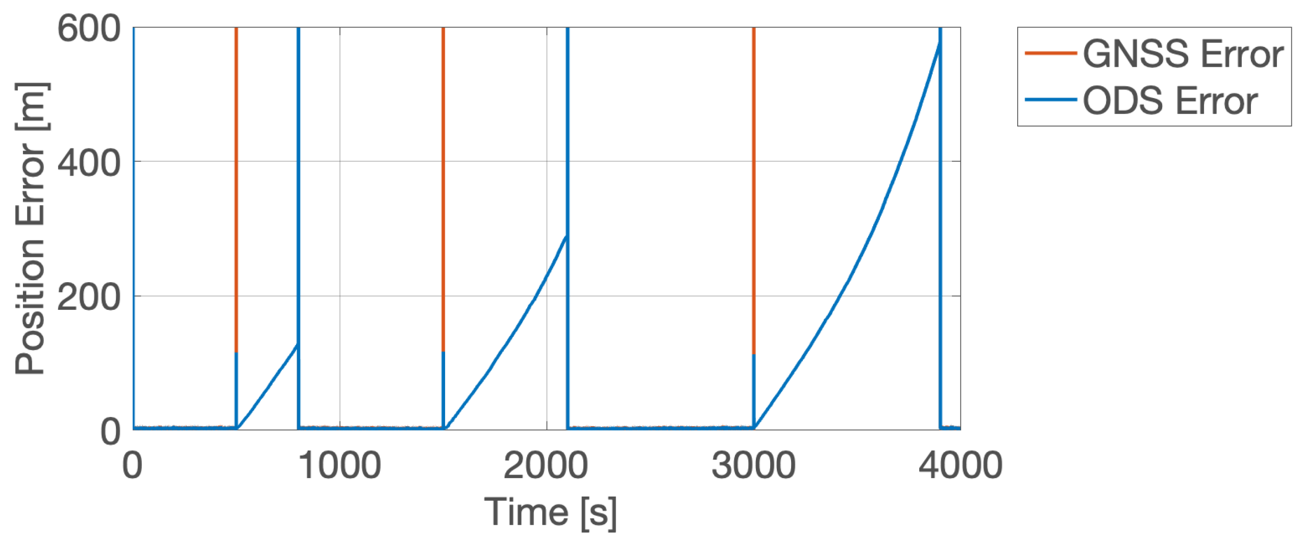
Figure 10 shows a MIL level verification of the ODS, where multiple GNSS outage periods are injected into the functional engineering simulator. Whenever the GNSS measurements are available, the ODS performance are the nominal one, already discussed in Figure 7. However, if the GNSS is not providing a valid position fix, the on-board orbital dynamics propagator is used as a synthetic measurement for the inertial navigation system. In this condition the bias estimates of the accelerometers are not updated, but the EKF is applied to merge orbital propagation and accelerometer data. The result is a slower divergence rate of the position error with respect to a pure on-board orbital propagation. With a tactical grade accelerometer for small satellite platforms, the propagation error is limited to ∼100 m for ∼
5 min of GNSS outage, ∼300 m for ∼10 min, and ∼600 m for ∼15 min. The position error increases more than linearly in the first propagation periods, but it tends to stabilize and oscillates around a steady state error value in the order of 1 to 10 km.
9. Discussion
The proposed fault tolerant attitude and orbit determination system (AODS) for small platforms has proven degree and meter level performances with typical sensors for small satellite platforms. The verification of the system has followed the guidelines based on international standards for model-in-the-loop verification of space software. The functional engineering simulator used for the verification campaign is based on validated dynamics and environment models, and the sensors models includes all the errors sources and the signal transduction problems. Despite this paper describes the sensor post processing from the raw signals of the measured physical quantities, the simulations include all the post processing operations to convert the sensor’s output in the measured quantity. The sensor post processing operations are needed to achieve the required performance with the components typically used in small spacecraft application. The performance of the AODS is maintained, with an acceptable level of degradation, after several failures have occurred to the components. The system level failure detection functions are capable to detect failures that, if propagated to the control subsystem, may pose the spacecraft in dangerous conditions. Moreover, the component level failure detection, combined with the system level management and reconfiguration, can mitigate the component failure propagation to the attitude and orbit estimation sections. The algorithms have proven their validity on a broad variety of component specifications for small spacecraft, through extensive simulation campaigns. The failure detection thresholds resulted to be the most sensitive variables to be accurately set for a given sensor and a given sensor combination.
Future works include a verification of the proposed AODS at the software and hardware-in-the-loop levels on relevant spacecraft components. The testing campaign shall begin from a broad characterization of nominal sensor performance to properly tune all the parameters and thresholds in the AODS. Then, the software-in-the-loop (SIL) testing campaign is conducted by combining the functional engineering simulator output with the software deployment of the AODS. This can be accomplished within the system deployment framework, which is capable of automatically running SIL tests on the auto-coded software. Eventually, the system shall undergo hardware-in-the-loop (HIL) testing phases. If a complete dynamical and environmental test bench is not available, the HIL tests can be run in hybrid mode. Namely, the sensor measurements are simulated in real-time and sent to the on-board computer through an interface subsystem modelling the hardware electrical and data interfaces. In this way the real-time execution and performance of the system are verified, without using a complex and expensive dynamical and environmental test bench. This verification approach is suitable for small satellite platforms, and it contributes to reducing the overall time and cost to space. Moreover, this approach with real-time simulated sensors is convenient for verifying and testing the fault tolerance performance of the AODS. In fact, the real-time simulator can include all the possible failures in the sensor measurements, without the need to stress real flight hardware. The major difficulty in this verification approach consists of the real-time simulation of realistic non-nominal and faulty behaviors of the sensors. However, literature data and hardware manufacturer experience may be exploited in setting up the simulation configuration.
The required computational load has been estimated to be feasible for typical on-board processors for small spacecraft. Preliminary processor-in-the-loop verification tests have confirmed this assumption. However, only a formal real-time verification of the proposed AODS at hardware level would certify it. This point is of primary relevance for the implementation of the proposed AODS in a real space system. In fact, the design of flight software for small satellite platforms shall be characterized by a small memory footprint and computational burden. However, this shall be compatible with the required functionalities and performance. The proposed fault tolerant AODS for small satellite platforms demonstrates a promising solution in this direction.
Author Contributions
Conceptualization, A.C.; methodology, A.C.; software, A.C.; validation, A.C.; formal analysis, A.C.; writing—original draft preparation, A.C.; writing—review and editing, A.C.; funding acquisition, M.L. All authors have read and agreed to the published version of the manuscript.
Funding
This research received no external funding.
Institutional Review Board Statement
Not applicable.
Informed Consent Statement
Not applicable.
Data Availability Statement
Not applicable.
Conflicts of Interest
The authors declare no conflict of interest. The funders had no role in the design of the study; in the collection, analyses, or interpretation of data; in the writing of the manuscript, or in the decision to publish the results.
References
- Raghunath, K.; Kang, J.S. An Exploration of the Small Satellite Value Chain and the Future of Space Access. In Proceedings of the AIAA/USU Conference on Small Satellites: Mission Operations & Autonomy, Virtual, 7–12 August 2021. Number SSC21-P1-29. [Google Scholar]
- ECSS. Space Engineering: Satellite Attitude and Orbit Control System (AOCS) Requirements; Technical Report ECSS-E-ST-60-30C; European Cooperation for Space Standardization: Paris, France, 2013. [Google Scholar]
- Perumal, R.P.; Voos, H.; Vedova, F.D.; Moser, H. Small Satellite Reliability: A decade in review. In Proceedings of the AIAA/USU Conference on Small Satellites: Mission Operations & Autonomy, Virtual, 7–12 August 2021. Number SSC21-WKIII-02. [Google Scholar]
- Colagrossi, A.; Prinetto, J.; Silvestrini, S.; Orfano, M.; Lavagna, M.; Fiore, F.; Burderi, L.; Bertacin, R.; Pirrotta, S. Semi-analytical approach to fasten complex and flexible pointing strategies definition for nanosatellite clusters: The HERMES mission case from design to flight. In Proceedings of the 70th International Astronautical Congress (IAC 2019), Washington, DC, USA, 21–25 October 2019; pp. 1–8. [Google Scholar]
- Colagrossi, A.; Silvestrini, S.; Prinetto, J.; Lavagna, M. HERMES: A CubeSat Based Constellation for the New Generation of Multi-Messenger Astrophysics. In Proceedings of the 2020 AAS/AIAA Astrodynamics Specialist Conference, Lake Tahoe, CA, USA, 9–12 August 2020; pp. 1–20. [Google Scholar]
- Markley, F. Attitude Determination Using Two Vector Measurements; Number NASA/CP-1999-209235; NASA Flight Mechanics Symposium: Washington, DC, USA, 1999; pp. 39–52. [Google Scholar]
- Wang, C.; Lachapelle, G.; Cannon, M.E. Development of an integrated low-cost GPS/rate gyro system for attitude determination. J. Navig. 2004, 57, 85–101. [Google Scholar] [CrossRef]
- Lefferts, E.; Markley, F.; Shuster, M. Kalman Filtering for Spacecraft Attitude Estimation. J. Guid. Control. Dyn. 1982, 5, 417–429. [Google Scholar] [CrossRef]
- Springmann, J.C.; Sloboda, A.J.; Klesh, A.T.; Bennett, M.W.; Cutler, J.W. The attitude determination system of the RAX satellite. Acta Astronaut. 2012, 75, 120–135. [Google Scholar] [CrossRef]
- Schmidt, M.; Ravandoor, K.; Kurz, O.; Busch, S.; Schilling, K. Attitude determination for the Pico-Satellite UWE-2. IFAC Proc. Vol. 2008, 41, 14036–14041. [Google Scholar] [CrossRef] [Green Version]
- Makovec, K.L.; Turner, A.J.; Hall, C.D. Design and implementation of a nanosatellite attitude determination and control system. In Proceedings of the 2001 AAS/AIAA Astrodynamics Specialists Conference, Quebec City, QC, Canada, 30 July–2 August 2001. Number AAS 01-311. [Google Scholar]
- Mahony, R.; Hamel, T.; Pflimlin, J.M. Complementary filter design on the special orthogonal group SO(3). In Proceedings of the 44th IEEE Conference on Decision and Control, Seville, Spain, 12–15 December 2005; pp. 1477–1484. [Google Scholar] [CrossRef] [Green Version]
- Mahony, R.; Hamel, T.; Pflimlin, J.M. Nonlinear complementary filters on the special orthogonal group. IEEE Trans. Autom. Control. 2008, 53, 1203–1218. [Google Scholar] [CrossRef] [Green Version]
- Dong, Y. MEMS inertial navigation systems for aircraft. In MEMS for Automotive and Aerospace Applications; Kraft, M., White, N.M., Eds.; Woodhead Publishing Series in Electronic and Optical Materials; Woodhead Publishing: Sawston, UK, 2013; pp. 177–219. [Google Scholar] [CrossRef]
- Wahba, G. A least squares estimate of satellite attitude. SIAM Rev. 1966, 7, 409. [Google Scholar] [CrossRef]
- Markley, F.L.; Mortari, D. Quaternion Attitude Estimation Using Vector Observations. J. Astronaut. Sci. 2000, 48, 359–380. [Google Scholar] [CrossRef]
- Shuster, M.D. The quest for better attitudes. J. Astronaut. Sci. 2006, 54, 657–683. [Google Scholar] [CrossRef]
- Alonso, R.; Shuster, M.D. TWOSTEP: A Fast Robust Algorithm for Attitude-Independent Magnetometer-Bias Determination. J. Astronaut. Sci. 2002, 50, 433–451. [Google Scholar] [CrossRef]
- Crassidis, J.L.; Lai, K.L.; Harman, R.R. Real-Time Attitude-Independent Three-Axis Magnetometer Calibration. J. Guid. Control. Dyn. 2005, 28, 115–120. [Google Scholar] [CrossRef]
- Titterton, D.; Weston, J.L.; Weston, J. Strapdown Inertial Navigation Technology; Institution of Engineering and Technology: London, UK, 2004. [Google Scholar]
- Vallado, D.A. Fundamentals of Astrodynamics and Applications; Springer Science & Business Media: Berlin, Germany, 2001. [Google Scholar]
- Jan, S.U.; Lee, Y.D.; Shin, J.; Koo, I. Sensor Fault Classification Based on Support Vector Machine and Statistical Time-Domain Features. IEEE Access 2017, 5, 8682–8690. [Google Scholar] [CrossRef]
- Ribeiro, M.I. Kalman and Extended Kalman Filters: Concept, Derivation and Properties; Institute for Systems and Robotics: Lisboa, Portugal, 2004; Volume 43. [Google Scholar]
- Carletta, S.; Teofilatto, P.; Farissi, M.S. A Magnetometer-Only Attitude Determination Strategy for Small Satellites: Design of the Algorithm and Hardware-in-the-Loop Testing. Aerospace 2020, 7, 3. [Google Scholar] [CrossRef] [Green Version]
Figure 1.
AODS architecture scheme.

Figure 2.
Sensor post processing scheme.

Figure 3.
Sensor faults and failure detection examples. (a) Spike fault; (b) Erratic fault; (c) Drift Fault; (d) Hardover Fault; (e) Data Loss Fault; (f) Stuck Fault.
Figure 3.
Sensor faults and failure detection examples. (a) Spike fault; (b) Erratic fault; (c) Drift Fault; (d) Hardover Fault; (e) Data Loss Fault; (f) Stuck Fault.


Figure 4.
Redundant component management example.

Figure 5.
Attitude error in MIL analysis of Earth pointing AODS, with continuous nadir rotation to align solar arrays.
Figure 5.
Attitude error in MIL analysis of Earth pointing AODS, with continuous nadir rotation to align solar arrays.

Figure 6.
Angular rates error in MIL analysis of Earth pointing AODS, with continuous nadir rotation to align solar arrays.
Figure 6.
Angular rates error in MIL analysis of Earth pointing AODS, with continuous nadir rotation to align solar arrays.

Figure 7.
Position error in MIL analysis of ODS.

Figure 8.
Reconfiguration and recalibration example.

Figure 9.
Attitude error in MIL analysis of Sun pointing AODS, with multiple injected failures. Gyroscopes loss at s. Primary magnetometer loss at 11,000 s. Sun sensors loss at 18,000 s.
Figure 9.
Attitude error in MIL analysis of Sun pointing AODS, with multiple injected failures. Gyroscopes loss at s. Primary magnetometer loss at 11,000 s. Sun sensors loss at 18,000 s.

Figure 10.
Position error in MIL analysis of ODS, with multiple GNSS outage periods: 5 min at s, 10 min at s, and 15 min at s.
Figure 10.
Position error in MIL analysis of ODS, with multiple GNSS outage periods: 5 min at s, 10 min at s, and 15 min at s.


Table 1.
Reconfiguration table examples.
| Failure | Reconfiguration Output | AODS Mode | ADCS Mode |
|---|---|---|---|
| Nominal mode: Earth pointing with reaction wheels. | |||
| Gyroscope 1 | Switch to redundant gyroscope 2 | FADS | Nominal |
| Gyroscope 1+2 | Switch to magnetometer angular rate estimation | FADS | Nominal |
| Magnetometer(s) | Transition to direct Sun pointing | SUNE | Safe |
| ODS | Transition to direct Sun pointing | SUNE | Safe |
| Gyroscope 1+2 and Magnetometer(s) | Transition to direct Sun pointing and ADCS stand-by in eclipse | SUNE | Safe |
| Nominal mode: Sun pointing with reaction wheels. | |||
| Fine Sun sensors | Switch to coarse Sun sensors | SUNE | Nominal |
| Sun sensors | Switch to solar array Sun estimation | SUNE | Nominal |
| Sun sensors and EPS communication | Transition to spinning attitude around solar arrays | AVES | Safe |
| Nominal mode: Detumbling with magnetic actuators. | |||
| Gyroscope(s) | Switch to magnetometer angular rate estimation | AVES | Nominal |
| Magnetometer(s) | Switch to detumbling with non-magnetic actuators | AVES | Nominal |
| Gyroscope(s) and Magnetometer(s) | ADCS stand-by, waiting for ground acknowledgement of a transition to direct Sun pointing, if angular rates allow it | N/A | Stand-by |
Publisher’s Note: MDPI stays neutral with regard to jurisdictional claims in published maps and institutional affiliations. |
© 2022 by the authors. Licensee MDPI, Basel, Switzerland. This article is an open access article distributed under the terms and conditions of the Creative Commons Attribution (CC BY) license (https://creativecommons.org/licenses/by/4.0/).
Share and Cite
MDPI and ACS Style
Colagrossi, A.; Lavagna, M. Fault Tolerant Attitude and Orbit Determination System for Small Satellite Platforms. Aerospace 2022, 9, 46. https://doi.org/10.3390/aerospace9020046
AMA Style
Colagrossi A, Lavagna M. Fault Tolerant Attitude and Orbit Determination System for Small Satellite Platforms. Aerospace. 2022; 9(2):46. https://doi.org/10.3390/aerospace9020046
Chicago/Turabian StyleColagrossi, Andrea, and Michèle Lavagna. 2022. "Fault Tolerant Attitude and Orbit Determination System for Small Satellite Platforms" Aerospace 9, no. 2: 46. https://doi.org/10.3390/aerospace9020046
Note that from the first issue of 2016, this journal uses article numbers instead of page numbers. See further details here.