Dynamic Burst Actuation to Enhance the Flow Control Authority of Plasma Actuators

Abstract

A computational study was conducted on flows over an NACA0015 airfoil with dielectric barrier discharge (DBD) plasma. The separated flows were controlled by a DBD plasma actuator installed at the 5% chord position from the leading edge, where operated AC voltage was modulated with the duty cycle not given a priori but dynamically changed based on the flow fluctuations over the airfoil surface. A single-point pressure sensor was installed at the 40% chord position of the airfoil surface and the DBD plasma actuator was activated and deactivated based on the strength of the measured pressure fluctuations. The Reynolds number was set to 63,000 and flows at angles of attack of 12 and 16 degrees were considered. The three-dimensional compressible Navier–Stokes equations including the DBD plasma actuator body force were solved using an implicit large-eddy simulation. Good flow control was observed, and the burst frequency proven to be effective in previous fixed burst frequency studies is automatically realized by this approach. The burst frequency is related to the characteristic pressure fluctuation; our approach was improved based on the findings. This improved approach realizes the effective burst frequency with a lower control cost and is robust to changing the angle of attack.

1. Introduction

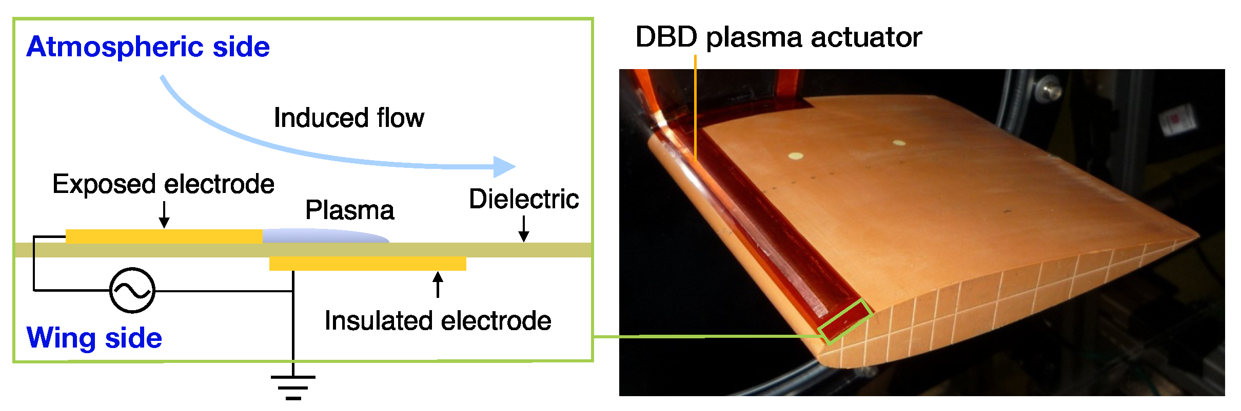
Flow separation control is an important topic of fluid dynamics and has been studied for many years. Small devices that control flow separations using plasma-induced body forces have recently received much attention because of their distinct advantages, such as simple structure, absence of mechanical systems, low power consumption, and quick response. One of these small devices specifically considered here is the dielectric barrier discharge (DBD) plasma actuator, which is schematically presented in Figure 1. Additionally shown in Figure 1 is an example of practical applications where a DBD plasma actuator is attached to the leading edge region of an airfoil model in the experiment. A typical DBD plasma actuator comprises two electrodes and one dielectric. It operates under an alternating current (AC) voltage with an amplitude of several kilovolts and frequencies of 1-20 kHz. When a high AC voltage is applied to the electrodes, the DBD plasma actuator generates plasma, which induces local jet-like flows from the exposed electrode toward the insulated electrode in the time-averaged flow field.

Early studies demonstrated that induced flows effectively control flow separations when the layout and device parameters are appropriately arranged [1,2]. Numbers of both experimental and computational studies and their reviews that appeared in the last 10 to 15 years are presented in [3,4,5,6,7,8,9,10,11,12,13,14,15,16,17,18,19]. Most of these studies focused on applications to airfoil flows at low Reynolds numbers ($Re={10}^4$–${10}^5$). Some of them investigated input AC parameters, such as operational voltage, frequency, and waveform, for better authority of flow control. In addition, some groups have investigated the use of duty cycles for better flow control [20,21]. The duty cycle is called “burst” actuation compared to the conventional “continuous” actuation without a duty cycle. Early studies indicated that a non-dimensional burst frequency around one was effective. The authors’ group conducted both experimental and computational investigations on the relationship between burst frequencies and flow control authority and showed that higher non-dimensional burst frequencies, such as 6 to 10, are much more effective under certain conditions, and identified that such frequencies are closely related to the instability of the separation shear layer [22,23,24,25]. They also identified three important flow structures: induced weak jets, two-dimensional vortex flow structures, and small disturbances in the burst actuation, which were key for robust flow control in burst actuation [26,27]. They suggested a method of choosing the effective burst frequencies based on their observations. However, this was a qualitative suggestion and depends on the flow and geometry conditions. There remain difficulties in choosing effective burst frequencies for a wide range of applications. In addition, the burst frequency should be dynamically optimized according to the instantaneous flow conditions when inflows are changed in time, as in the case of wind turbines. In the present study, we propose a method in which the on/off duty is automatically optimized by a simple feedback loop using a single-point pressure sensor located over the airfoil surface. The effectiveness of the method is discussed based on high-fidelity computations using large-eddy simulations (LES) with the actuator-induced body force added. This method may be considered as a control system which optimizes the time-dependent burst frequencies with the measured unsteady pressure data over the airfoil surface. Benard et al. used feedback loop control for DBD plasma actuators. They focused on AC voltage optimization to reduce the electric power consumption [28]. However, few studies have focused on feedback loop control for DBD plasma actuators.

In this study, dynamic burst actuation for the enhancement of the flow control authority of plasma actuators is proposed. To identify the effectiveness of the dynamic burst actuation, the three-dimensional compressible Navier–Stokes equations with the DBD plasma actuator body force terms were solved by an implicit large-eddy simulation (iLES), and the results are discussed. The plasma actuator was installed at a 5% chord position from the leading edge of the airfoil with a cross-section of an NACA0015 airfoil. The Reynolds number was set to 63,000, and post-stall angles of attack of $\alpha =12$ or 16 degrees were considered. A single-point pressure sensor was installed at a 40% chord position in the middle of the airfoil span. The separated flows were controlled by the DBD plasma actuator, where the AC voltage was modulated with the duty cycle not given a priori, but dynamically changed based on the measured pressure fluctuations given by the point sensor. Two modulation strategies were considered [29,30]. The present approach realizes effective dynamic burst frequency automatically with little additional cost. Application to the case at a higher angle of attack highlighted the robustness of one of the approaches presented here.

2. Burst Actuations

2.1. Classic Burst Actuation

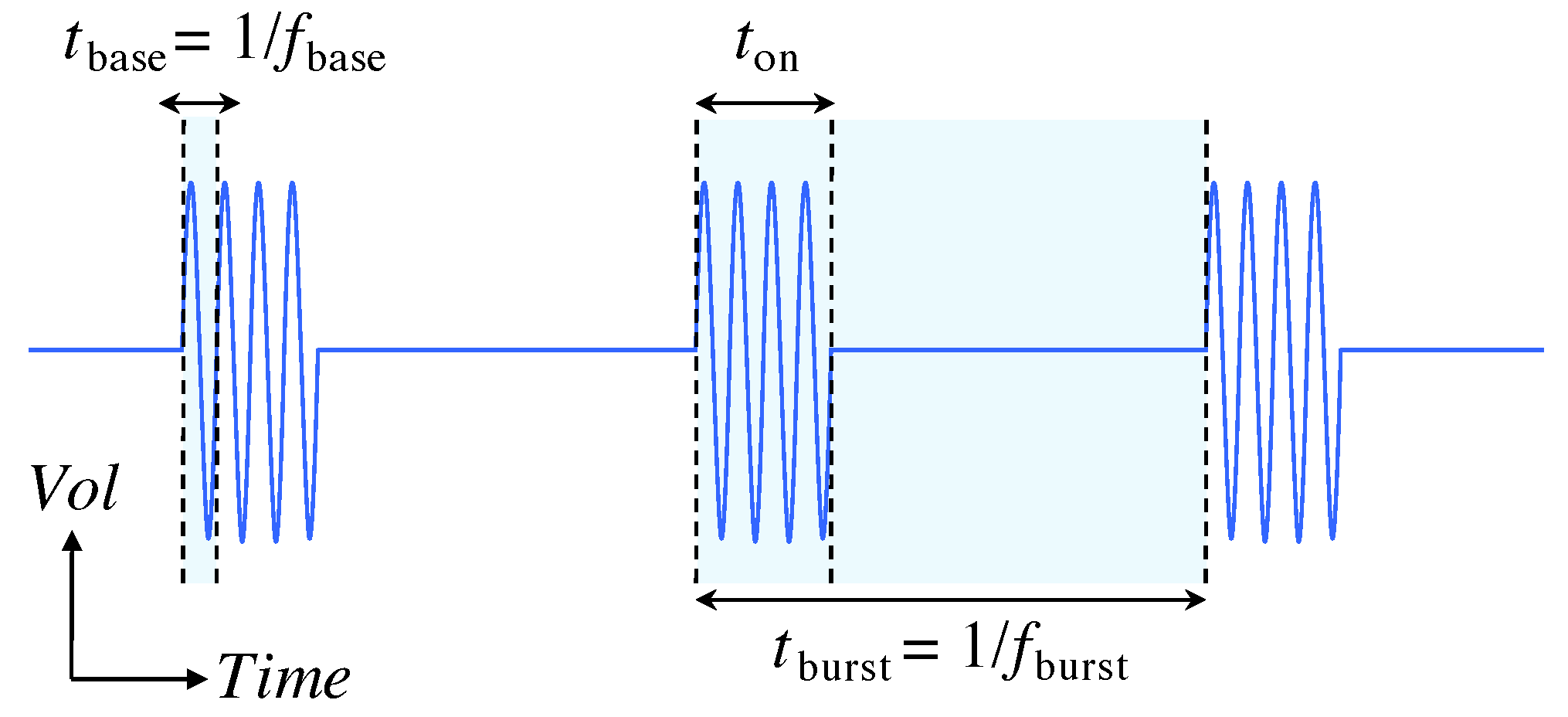
Burst actuation is a method of driving a plasma actuator. The AC voltage modulated with the duty cycle is applied to the plasma actuator during burst actuation. Previous studies [23,27] have shown that burst actuation controls flow separations more efficiently than continuous actuation at low Reynolds numbers ($Re\simeq {10}^4$–${10}^5$). Figure 2 shows a schematic diagram of the AC voltage waveform for the burst actuation. Parameters of the waveform are defined as Equation (1). $f_{\mathrm{base}}$ is the base frequency of the AC voltage. $t_{\mathrm{on}}$, and $t_{\mathrm{burst}}$ are the driving time and burst period, respectively. $f_{\mathrm{burst}}$ denotes the burst frequency. $F^{+}$, $F_{\mathrm{base}}$, and $BR$ are non-dimensional $f_{\mathrm{burst}}$, non-dimensional $f_{\mathrm{base}}$, and burst ratio, respectively.

$$\begin{array}{c}\hfill F^{+}=\frac{f_{\mathrm{burst}}c}{U_{\infty }},F_{\mathrm{base}}=\frac{f_{\mathrm{base}}c}{U_{\infty }},BR=\frac{t_{\mathrm{on}}}{t_{\mathrm{burst}}}.\end{array}$$

(1)

The authors’ group showed that the appropriate $F^{+}$ had to be chosen according to the flow conditions: that is, $F^{+}\simeq 10$ at the near-stall condition and $F^{+}\simeq 1$ under the conditions of deep stall or a higher Reynolds number ($Re\simeq {10}^6$) [27]. In burst actuation, two-dimensional (spanwise) vortices are generated by the plasma actuator. The spanwise vortices generated by the burst actuation of $F^{+}\simeq 10$ break down into three-dimensional vortices as they move downstream, promoting flow mixing and suppressing flow separation. In contrast, the spanwise vortices emitted by the burst actuation of $F^{+}\simeq 1$ are relatively large, and the vortex structure is maintained downstream. The advection of those vortices suppresses the separation of flow. A detailed discussion may be found in the related papers [26,27]. The separation control mechanism is different for different values of $F^{+}$, and the effective $F^{+}$ for the separation control differs depending on the flow conditions. Although previous studies have provided some guidelines for choosing $F^{+}$, these were qualitative suggestions for limited static conditions. For practical conditions, the burst frequency should be dynamically determined. Therefore, the authors’ group is developing methods that dynamically change $F^{+}$, hereafter termed as “dynamic burst” actuation.

2.2. Dynamic Burst Actuation

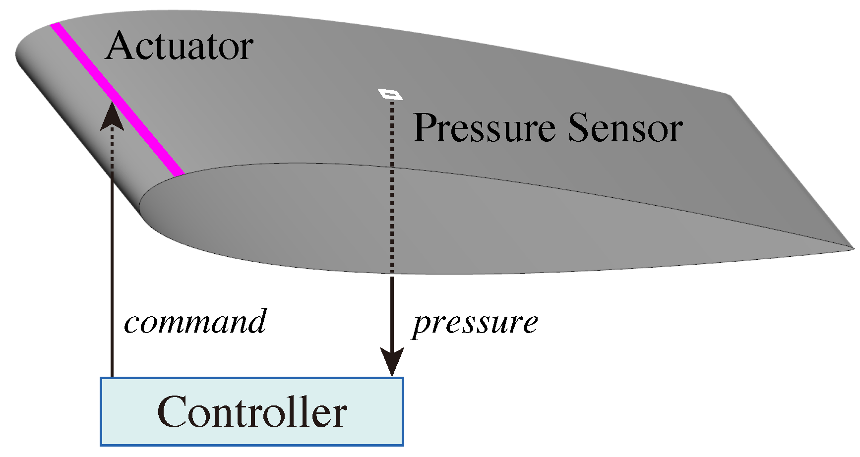
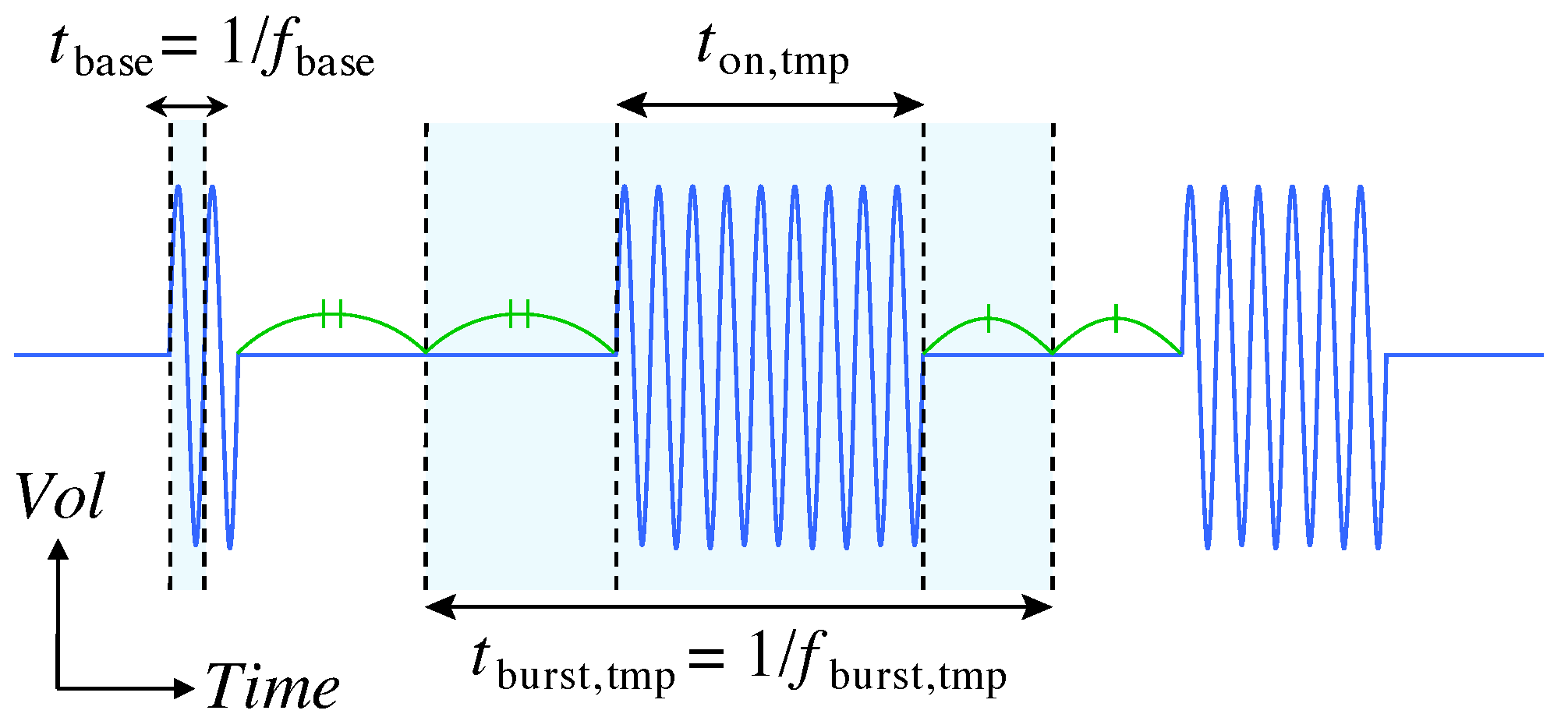
Figure 3 shows a schematic diagram of the dynamic burst actuation. As mentioned in Section 2.1, when separation control by the burst actuation is effectively performed, spanwise vortices according to $F^{+}$ are generated on the airfoil surface, and its advection downstream plays an important role in the separation control. Dynamic burst actuation dynamically changes $F^{+}$ by detecting the advection of these vortices on the airfoil surface. In the present method, a single pressure sensor was used to detect the vortex passing on the airfoil surface. The pressure sensor was installed on the airfoil surface and connected to the plasma actuator through a controller. In the present study, the plasma actuator and pressure sensor were installed at 5% and 40% of the leading edge, respectively. The pressure sensor measures the instantaneous pressure and sends the value to the controller. A pressure sensor with a high time resolution, such as the Endevco Model 8507C-1 used in the experiments, is imitated in the computations. The measured surface pressure over the airfoil is used as the sensor measuring value. The controller sends on/off commands based on time-series pressure data to the plasma actuator. As a result of the on/off operation of the plasma actuator, $F^{+}$ is dynamically changed. Figure 4 shows the voltage waveform of the dynamic burst actuation. Each waveform parameter is defined by Equation (2). $t_{\mathrm{on},\mathrm{tmp}}$ and $t_{\mathrm{burst},\mathrm{tmp}}$ are the time duration when the plasma actuator is on and the temporary burst period, respectively. The start and end times of $t_{\mathrm{burst},\mathrm{tmp}}$ are intermediate times of the off duration before and after $t_{\mathrm{on},\mathrm{tmp}}$, respectively. $f_{\mathrm{burst},\mathrm{tmp}}$ denotes the temporary burst frequency. $F_{\mathrm{tmp}}^{+}$ and $B{R}_{\mathrm{tmp}}$ are the non-dimensional temporary burst frequencies and burst ratios, respectively.

$$\begin{array}{c}\hfill F_{\mathrm{tmp}}^{+}=\frac{f_{\mathrm{burst},\mathrm{tmp}}c}{U_{\infty }},B{R}_{\mathrm{tmp}}=\frac{t_{\mathrm{on},\mathrm{tmp}}}{t_{\mathrm{burst},\mathrm{tmp}}}.\end{array}$$

(2)

In this study, we investigated two types of controllers. The details of each controller are explained in Section 4 and Section 5. The time step width of the pressure measurement ($\Delta t_{\mathrm{sens}}$) and the time step width of the command ($\Delta t_{\mathrm{cmd}}$) were set to be 0.001 according to the performance of the realistic experimental equipment. When the plasma actuator receives the off command, if the base AC voltage is not zero, the plasma actuator turns off in the phase when the base AC voltage becomes zero in the next cycle.

3. Computational Approach

3.1. Governing Equations

Three-dimensional compressible Navier–Stokes equations with the source term added were solved in this study. The equations are non-dimensionalized by the free-stream density, free-stream velocity, and chord length of the airfoil and are represented as follows:

$$\begin{array}{ccc}\hfill \frac{\partial \rho }{\partial t}+\frac{\partial \rho u_j}{\partial x_j}& =& 0,\hfill \end{array}$$

(3)

$$\begin{array}{ccc}\hfill \frac{\partial \rho u_i}{\partial t}+\frac{\partial \left(\rho u_i{u}_j+p{\delta }_{ij}\right)}{\partial x_j}& =& \frac{1}{Re}\frac{\partial {\tau }_{ij}}{\partial x_j}+D_{\mathrm{c}}{S}_i,\hfill \end{array}$$

(4)

$$\begin{array}{ccc}\hfill \frac{\partial e}{\partial t}+\frac{\partial \left(\left(e+p\right)u_j\right)}{\partial x_j}& =& \frac{1}{Re}\frac{\partial u_k{\tau }_{jk}}{\partial x_j}-\frac{1}{\left(\gamma -1\right)PrRe{M}_{\infty }^2}\frac{\partial q_j}{\partial x_j}+D_{\mathrm{c}}{S}_j{u}_j,\hfill \end{array}$$

(5)

where $x_i$, $u_i$, $q_i$, $\rho$, p, e, ${\tau }_{ij}$, and t denote the non-dimensional forms of the position vector, velocity vector, heat flux vector, density, pressure, energy per unit volume, stress tensor, and time, respectively. ${\delta }_{ij}$ is the Kronecker delta. Equations (3)–(5) follow Einstein notation. Subscript i is a free index, and j and k are dummy indices. The indices take of values 1, 2, or 3. $Re$, $M_{\infty }$, and $Pr$ denote the Reynolds number, free-stream Mach number, and Prandtl number, respectively. They are defined as follows:

$$\begin{array}{c}\hfill Re=\frac{{\rho }_{\infty }{U}_{\infty }c}{{\mu }_{\infty }},M_{\infty }=\frac{U_{\infty }}{a_{\infty }},Pr=\frac{{\mu }_{\infty }{c}_{\mathrm{p}}}{{\kappa }_{\infty }},\end{array}$$

(6)

where ${\mu }_{\infty }$, ${\rho }_{\infty }$, $U_{\infty }$, c, $a_{\infty }$, $c_{\mathrm{p}}$, and ${\kappa }_{\infty }$ denote the viscosity, density, velocity, chord length, sound speed, constant pressure specific heat, and heat conduction coefficient, respectively. Here, a quantity with subscript ∞ denotes the quantity in the free-stream condition. The viscosity is calculated using Sutherland’s law. In Equations (4) and (5), the last terms on the right-hand side correspond to body force and power added to the unit volume by the plasma actuator, respectively. Hereinafter, for ease of understanding, x, y, z, u, v, and w represent the position and flow velocity of $x_1$, $x_2$, $x_3$, $u_1$, $u_2$, and $u_3$, respectively. In the present study, the free-stream Mach number is set to 0.2 to make the compressibility of fluid almost negligible, which reduces the computational cost using a larger time step size. Therefore, notably, the Mach numbers in the present study and previous experimental studies [22,23] are different. The specific heat ratio and Prandtl number were set to 1.4 and 0.72, respectively.

3.2. Plasma Actuator Modeling

The body force term for the plasma actuator was modeled with $D_{\mathrm{c}}{S}_i$ and $D_{\mathrm{c}}{S}_j{u}_j$ in the Navier–Stokes equations, as in Equations (4) and (5). The Suzen–Huang model [31] is utilized to obtain $S_i$. The non-dimensional body force vector $S_i$ is represented as follows:

$$S_i={\rho }_{\mathrm{c}}\left(-{\displaystyle \frac{\partial \varphi }{\partial x_i}}\right)f{\left(t\right)}^2,$$

(7)

where $f\left(t\right)$ is the waveform function of the input voltage, ${\rho }_{\mathrm{c}}$ is the net charge density, and $\varphi$ is the electric potential. The following equations are solved to obtain ${\rho }_{\mathrm{c}}$ and $\varphi$:

$$\begin{array}{ccc}\hfill {\displaystyle \frac{\partial }{\partial x_j}}\left({\epsilon }_{\mathrm{r}}{\displaystyle \frac{\partial \varphi }{\partial x_j}}\right)& =& 0,\hfill \end{array}$$

(8)

$$\begin{array}{ccc}\hfill {\displaystyle \frac{\partial }{\partial x_j}}\left({\epsilon }_{\mathrm{r}}{\displaystyle \frac{\partial {\rho }_{\mathrm{c}}}{\partial x_j}}\right)& =& {\displaystyle \frac{{\rho }_c}{{\lambda }_{\mathrm{d}}^2}},\hfill \end{array}$$

(9)

where ${\epsilon }_{\mathrm{r}}$ is the relative permittivity of the medium, and ${\lambda }_{\mathrm{d}}$ is the Debye length.

The following plasma actuator is considered in the present study: The exposed electrode is 2 mm wide, and the insulated electrode is $8.75$ mm wide. The electrodes are $0.1$ mm thick and separated by a $0.1$ mm thick dielectric. The streamwise spacing of electrodes is $0.5$ mm. The dielectric is Kapton, and ${\epsilon }_{\mathrm{r}}$ is 2.7. In the air, ${\epsilon }_{\mathrm{r}}$ is 1.0. For ${\lambda }_{\mathrm{d}}$, the same 1 mm as in the previous study is used [31]. These length parameters are non-dimensionalized by the reference length $c=0.1$ m. Equations (8) and (9) are solved by the successive over-relaxation (SOR) method using a $1201\times 801$ two-dimensional mesh. The boundary conditions for Equation (8) are given as follows:

$$\begin{array}{cc}\mathrm{on} \mathrm{outer} \mathrm{boundaries},\hfill & \partial \varphi /\partial n_i=0,\hfill \\ \mathrm{on} \mathrm{exposed} \mathrm{electrode},\hfill & \varphi =1.0,\hfill \\ \mathrm{on} \mathrm{insulated} \mathrm{electrode},\hfill & \varphi =0,\hfill \end{array}$$

where $n_i$ is the unit normal vector. The boundary conditions for Equation (9) are given as:

$$\begin{array}{cc}\mathrm{on} \mathrm{outer} \mathrm{boundaries} \mathrm{and} \mathrm{in} \mathrm{dielectric},\hfill & {\rho }_{\mathrm{c}}=0,\hfill \\ \mathrm{on} \mathrm{the} \mathrm{surface} \mathrm{of} \mathrm{dielectric} \mathrm{above} \mathrm{the} \mathrm{insulated} \mathrm{electrode},\hfill & {\rho }_{\mathrm{c}}=G\left(x^{\prime }\right),\hfill \\ \mathrm{on} \mathrm{the} \mathrm{other} \mathrm{surface} \mathrm{of} \mathrm{the} \mathrm{plasma} \mathrm{actuator},\hfill & \partial {\rho }_{\mathrm{c}}/\partial n_i=0.\hfill \end{array}$$

$G\left(x^{\prime }\right)$ is given by a half Gaussian distribution as follows:

$$G\left(x^{\prime }\right)=\exp \left(-{\displaystyle \frac{{x^{\prime }}^2}{2{\delta }^2}}\right),$$

(10)

where $x^{\prime }$ is the chordwise length measured from the edge of the insulated electrode, and $\delta$ is set to $0.3l_{\mathrm{e}}$ in this study. $l_{\mathrm{e}}$ is the insulated electrode length. In the present study, the input voltage is a standard alternating current. Therefore, the waveform $f\left(t\right)$ is the sinusoidal wave:

$$f\left(t\right)=\sin \left(2\pi F_{\mathrm{base}}t\right).$$

(11)

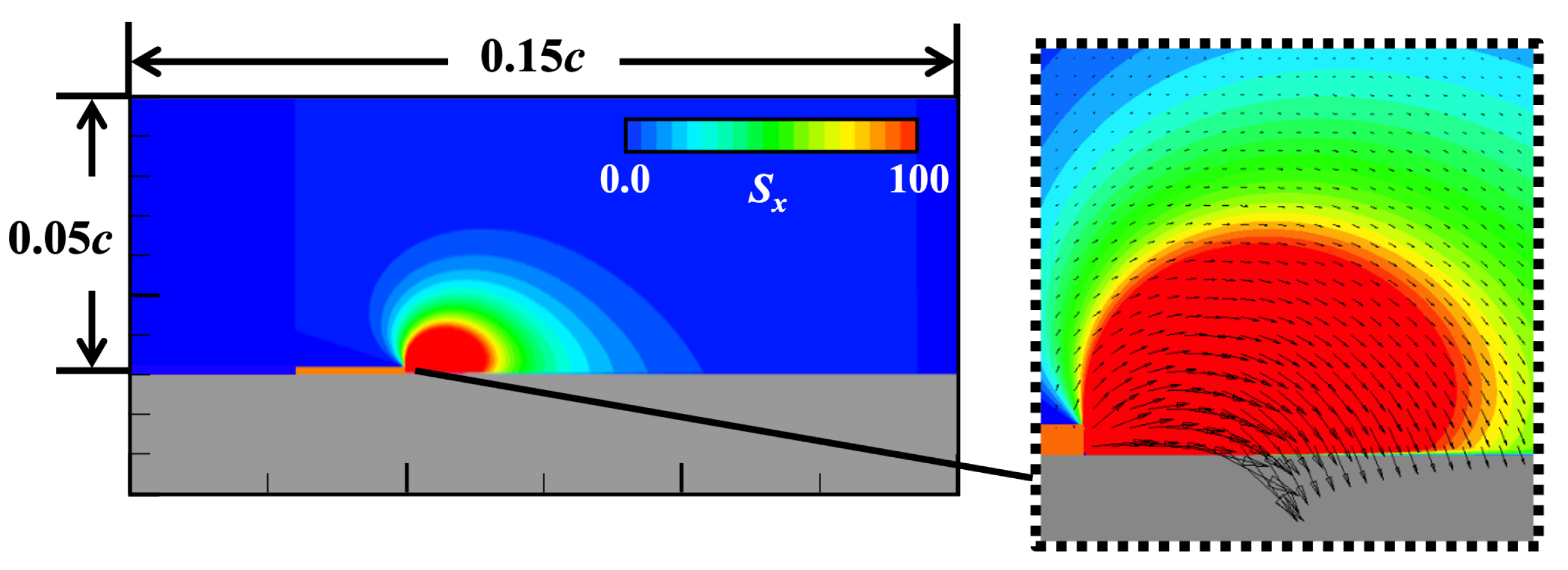
Figure 5 shows the distribution of the body force magnitude in the x direction ($S_x$) when $f\left(t\right)=1$. The body force vectors are also shown in an enlarged view near the actuator. The length of the model region is $0.15c$ in the chordwise direction and $0.05c$ in the wall-normal direction. The body force in the spanwise direction was not implemented so that no disturbance in the spanwise direction could be included in the plasma actuation of the present simulations. The magnitude of the body force is determined by the non-dimensional input voltage parameter, $D_c$, which is defined as follows:

$$\begin{array}{c}\hfill D_{\mathrm{c}}={\displaystyle \frac{{\rho }_{\mathrm{c},\max }{\varphi }_{\max }}{{\rho }_{\infty }{U}_{\infty }^2}},\end{array}$$

(12)

where ${\rho }_{\mathrm{c},\max }$ and ${\varphi }_{\max }$ are the maximum values of ${\rho }_{\mathrm{c}}$ and $\varphi$. In the present study, $D_{\mathrm{c}}=0.04$ is used. The maximum induced velocity produced by continuous actuation with $D_{\mathrm{c}}=0.04$ in quiescent air reaches approximately $3.4$ m/s if the reference velocity is $U_{\infty }=10$ m/s [32]. This value is equivalent to the induced velocity produced by the plasma actuator with a peak-to-peak applied voltage of 9 kV [19]. In the present body force model, the fluctuation is modeled by the square of the sinusoidal function. The direction of the body force produced by this fluctuation does not change within a single AC cycle, and even if the phase of the AC voltage changes, the body force in the opposite direction is not generated. This characteristic is similar to that of the “push–push type” model suggested by Font et al. [33]. $F_{\mathrm{base}}$ was set to 60, which corresponds to the frequency used in previous experiments [22,23]. Although the present model is simple, we validated it by comparing the LES results and the experimental results [24]. In addition, we also confirmed that the LES results using this model were not significantly different from those using a high-fidelity model [34].

The obtained body force is mapped to the computational grid for LES after rotating around the downstream edge of the exposed electrode to match the tangential direction of the airfoil surface.

3.3. Computational Method

We employ the flow solver LANS3D, which has been developed and verified to achieve high-fidelity simulation [35,36,37]. Generalized curvilinear coordinates ($\xi ,\eta ,\zeta$) were adopted to solve the governing equations. The spatial derivatives of the convective and viscous terms, metrics, and Jacobian were evaluated using a sixth-order compact difference scheme [38]. At the first and second points off the wall boundary, a second-order explicit difference scheme was adopted. Tenth-order filtering [38,39] was used with a filtering coefficient of 0.495. A backward second-order difference formula was used for time integration, and five sub-iterations [40] were adopted to ensure time accuracy. For time integration, the lower-upper symmetric alternating direction implicit and symmetric Gauss–Seidel (ADI-SGS) [41] methods were used. The time step size non-dimensionalized by the free-stream velocity and the chord length was $4\times {10}^{-5}$. The maximum Courant number was approximately 2.0. The non-dimensional time step based on the wall units was lower than 0.025 at the attached turbulent boundary layer. Choi and Moin [42] indicated that a time step of less than 0.4 is sufficient for the LES on a turbulent boundary layer. In contrast, additional stress and heat flux sub-grid modeling terms are implemented in an ordinary LES approach; they are not implemented in an iLES approach. In the present study, based on the supposition that a high-order lowpass filter selectively damps only unresolved high-frequency waves, an iLES was employed. Therefore, the present simulations do not use additional stress and heat flux terms based on standard sub-grid scale models.

At the outflow boundary, all variables were extrapolated from one point inside the outflow boundary. Here, the static pressure was fixed as that of the free-stream. No-slip and adiabatic conditions were adopted at the wall boundary. A periodic boundary condition was used for the boundaries in the spanwise direction. A uniform flow with no disturbance was used as the inflow condition.

A message passing interface was employed for parallel computing. All LESs were performed using the JAXA Supercomputer System Generation 2 (JSS2) at the Japan Aerospace Exploration Agency. Approximately 80 nodes (2560 cores) were used for each case.

3.4. Computational Grid

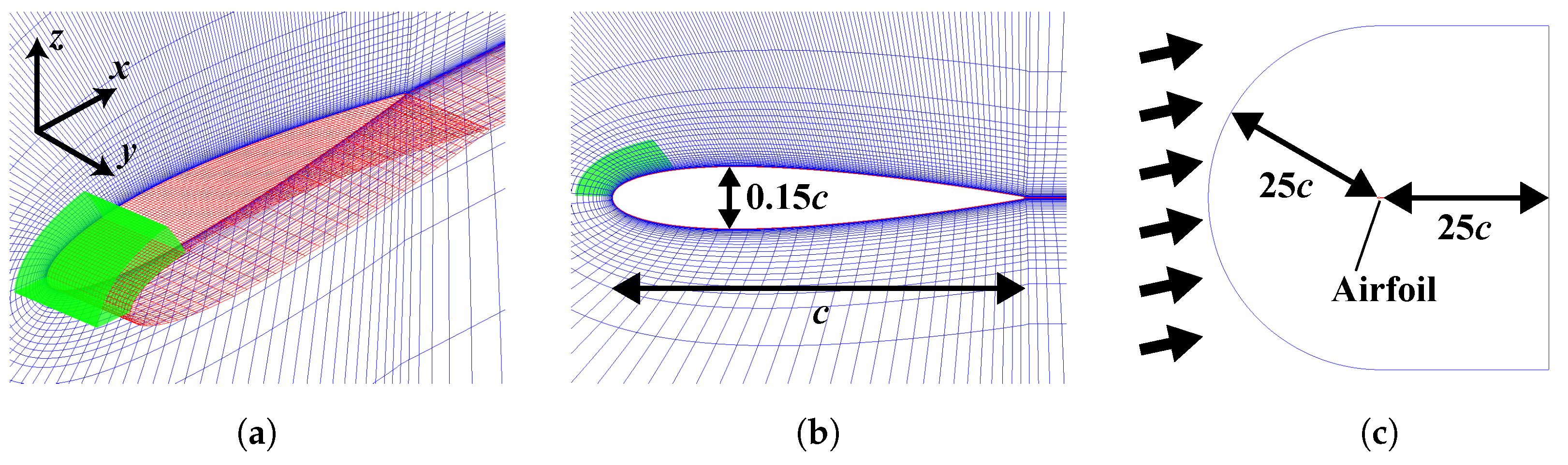
Two computational grids with different resolutions and the zonal method [43] were employed to treat the small fluid fluctuations induced by the body force of the plasma actuator. Figure 6 shows the computational grids and the computational domain with a schematic diagram of the inflow. The computational grids consist of an airfoil grid (zone 1: blue and red) and a fine actuator grid (zone 2: green). The computation procedure consists of the following three steps. First, the body force of the Suzen–Huang model is calculated on an ultra-fine grid corresponding to the body force model region. Second, the body force obtained in the previous step is mapped to the zone 2 grid from the ultra-fine grid. Finally, Equations (3)–(5) are solved for zones 1 and 2, and the physical values are interpolated from each other. Here, we used a C-type grid for the airfoil zone. The distances from the airfoil surface to the exterior boundary and the span length were $25c$ and $0.2c$, respectively. The airfoil and the plasma actuator zone have approximately $1.8\times {10}^7$ and $2.0\times {10}^6$ grid points, respectively, as shown in

Table 1. Number of computational grid points.

	$\mathit{\xi }$	$\mathit{\eta }$	$\mathit{\zeta }$	Total Point
Zone 1	759	134	179	18,205,374
Zone 2	149	134	111	2,216,226

. The minimum grid size in the wall-normal direction is $0.00012c$. The maximum grid spacing based on the wall unit at the attached turbulent boundary layer region is $(\Delta {\xi }^{+},\Delta {\eta }^{+},\Delta {\zeta }^{+})\lesssim (8,9,1)$. The present grid resolution and the computational methods are validated in the previous study [24].

4. Fixed Threshold Method (FTM)

4.1. Introduction of the FTM

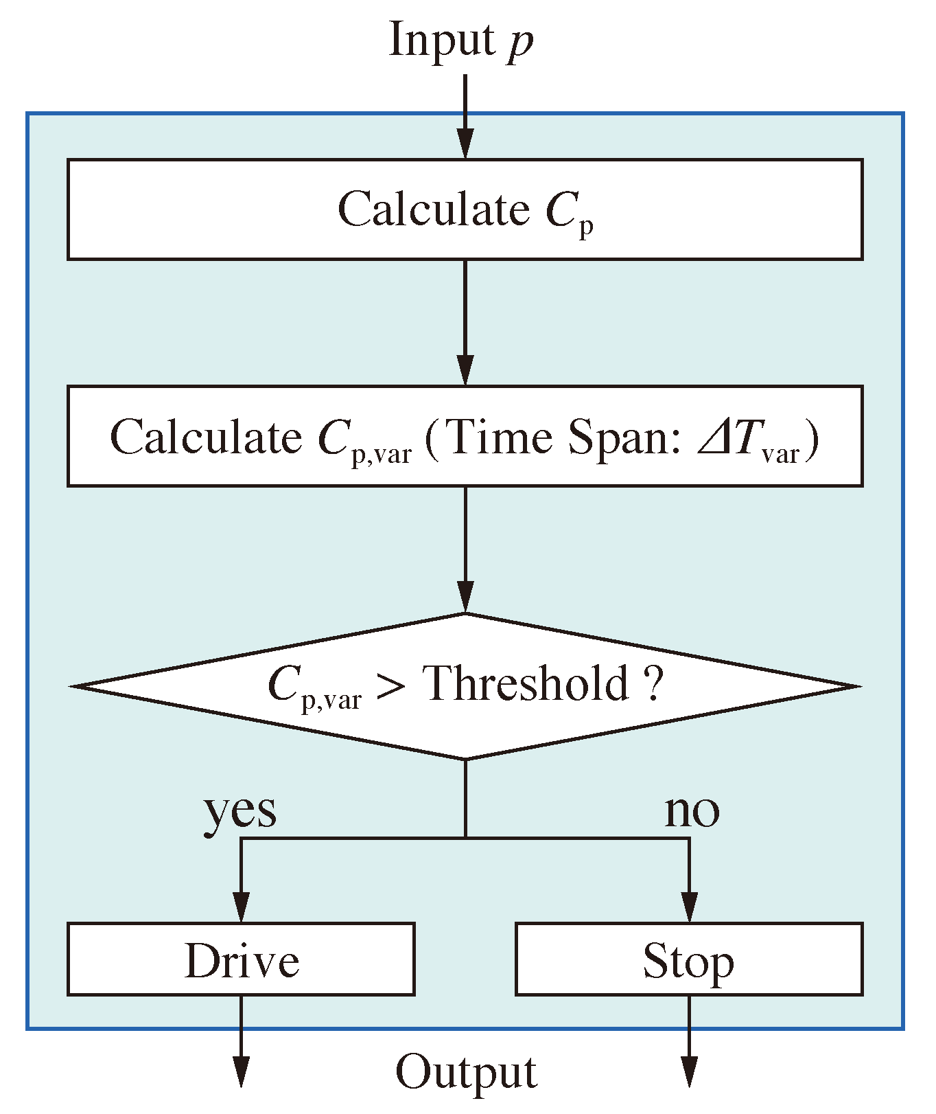
In this section, the FTM, which was first proposed for dynamic burst actuation, is investigated. Figure 7 shows the FTM flowchart. The controller receives an instantaneous pressure value from a single pressure sensor and stores time-series data. At the controller, the variance of the instantaneous pressure ($C_{\mathrm{p},\mathrm{var}}$) is computed based on the pressure through the following equations:

$$\begin{array}{cc}\hfill C_{\mathrm{p},\mathrm{var}}\left(t_n\right)& =\frac{1}{N}\left\{\sum _{i=1}^N{C}_{\mathrm{p}}{\left(t_i\right)}^2-{\left(\sum _{i=1}^N{C}_{\mathrm{p}}\left(t_i\right)\right)}^2\right\}\left(t_n\ge \Delta T_{\mathrm{var}}\right),\hfill \end{array}$$

(13)

$$\begin{array}{cc}\hfill C_{\mathrm{p}}\left(t_i\right)& ={\displaystyle \frac{p\left(t_i\right)-p_{\infty }}{{\displaystyle \frac{1}{2}}\rho {U_{\infty }}^2}},\hfill \end{array}$$

(14)

$$\begin{array}{cc}\hfill t_i& =(n-N+i)\Delta t_{\mathrm{sens}},\hfill \end{array}$$

(15)

$$\begin{array}{cc}\hfill N& ={\displaystyle \frac{\Delta T_{\mathrm{var}}}{\Delta t_{\mathrm{sens}}}}+1,\hfill \end{array}$$

(16)

where $t_n$ denotes the n-th sample time in the time step $\Delta t_{\mathrm{sens}}$, i.e., $t_n=n\Delta t_{\mathrm{sens}}$. The time duration ($\Delta T_{\mathrm{var}}$) for calculating $C_{\mathrm{p},\mathrm{var}}$ is set to 0.02. Then, the plasma actuator’s driving state (on/off) is determined by comparing $C_{\mathrm{p},\mathrm{var}}$ with the threshold value. The plasma actuator is turned on when $C_{\mathrm{p},\mathrm{var}}$ exceeds a certain fixed value (threshold), whereas the plasma actuator is turned off when $C_{\mathrm{p},\mathrm{var}}$ is lower than the threshold value, which is set in advance.

Table 2. Setting for fixed threshold of FTM.

Case	Fixed Threshold
FTM1	0.0001
FTM2	0.0005
FTM3	0.001
FTM4	0.002
FTM5	0.005

shows the threshold values used in the present simulations. These thresholds were chosen with reference to the $C_{\mathrm{p},\mathrm{var}}$ value of the case without the plasma actuator at $\alpha =12$. In Section 4.2, the effect of the threshold is investigated by simulations of the flow at $\alpha =12$.

4.2. Effect of the FTM Threshold

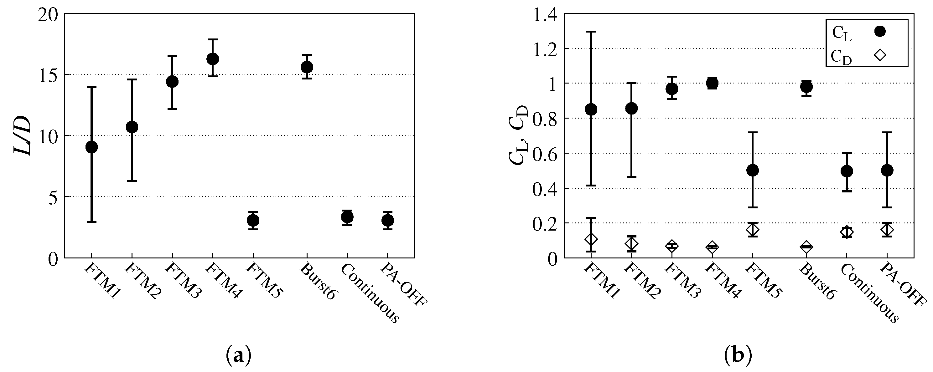
Figure 8 shows the aerodynamic characteristics in each FTM case and the previous computational results (Burst6, Continuous, and PA-OFF) [24] at $\alpha =12$. Burst6 is the classic burst actuation case with $BR=0.1$ and $F^{+}=6$, which is the effective burst frequency for flow separation control at $\alpha =12$. Continuous and PA-OFF are the continuous actuation case and the case without control of the plasma actuator, respectively. The symbols and error bars represent the mean values and upper and lower limits of the lift-to-drag ratio ($L/D$) and the lift and drag coefficients ($C_L,C_{\mathrm{D}}$), respectively. FTM cases improve the aerodynamic characteristics according to the threshold. Increasing the threshold from the FTM1 value to the FTM4 value increases $C_{\mathrm{L}}$, decreases $C_{\mathrm{D}}$, and thus, increases $L/D$. In addition, these fluctuations also become small. FTM4 has the highest $L/D$, which is 1.1 times larger than that of Burst6, which is known as an effective burst actuation. In contrast, in FTM5, the plasma actuator is mostly turned off because the threshold value is too high against the pressure fluctuation, and the $L/D$ is approximately the same as PA-OFF. As shown in Figure 8, the FTM improves the $L/D$, $C_{\mathrm{L}}$, and $C_{\mathrm{D}}$. However, its effects depend strongly on the setting of the fixed threshold. Although the simulation with the threshold FTM4, which was the most effective at $\alpha =12$, was also performed at $\alpha =16$, the FTM controller did not turn on the plasma actuator because the separated region was too large to detect vortex passing. As a result, the aerodynamic characteristics were almost identical to those of PA-OFF.

4.3. Relationship between Flow Field and Drive Status of the FTM

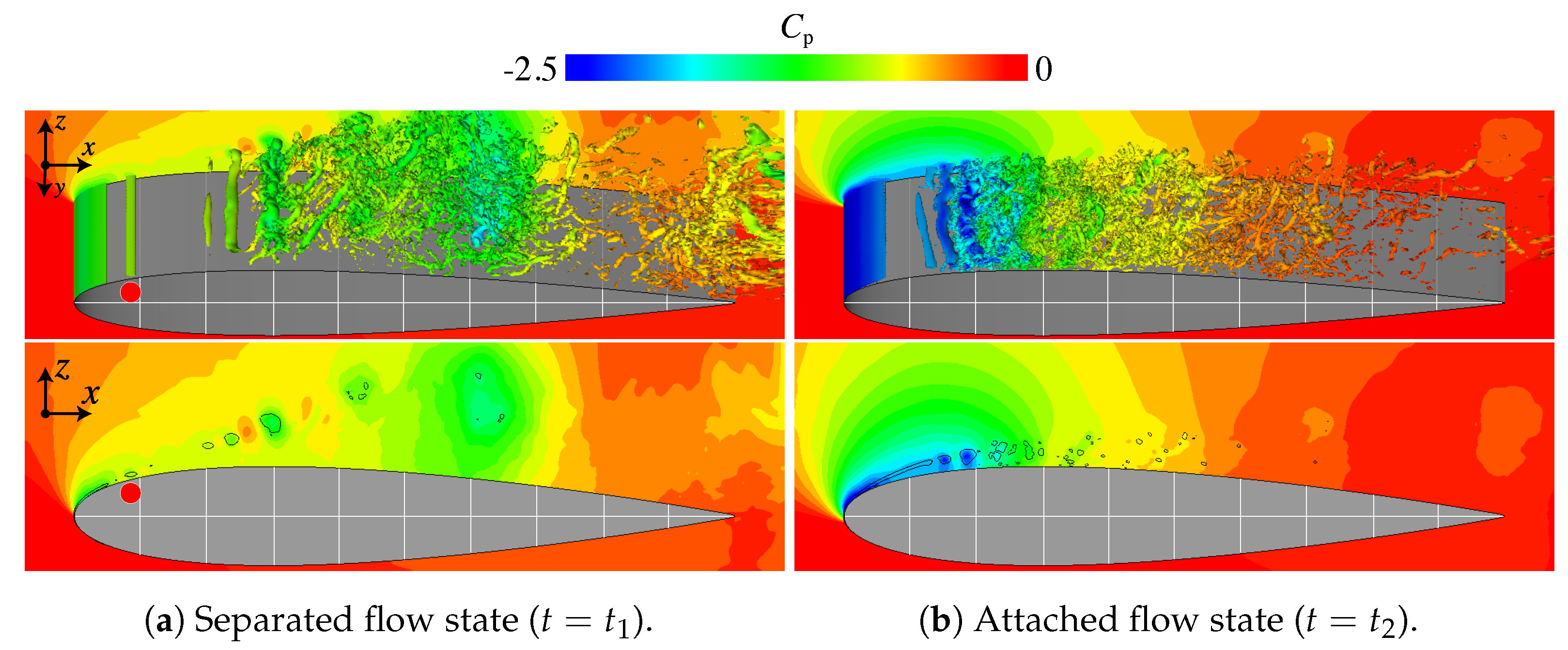
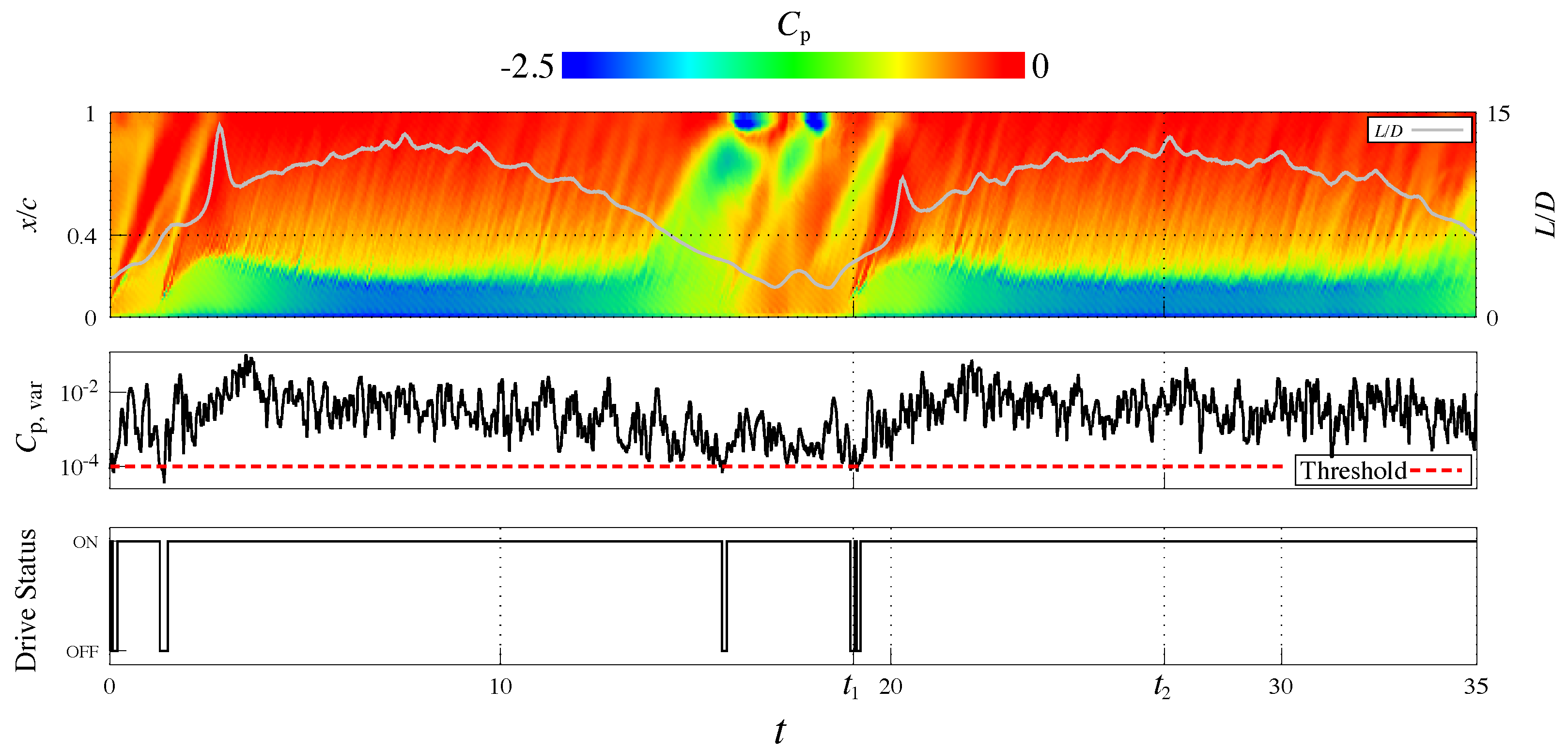
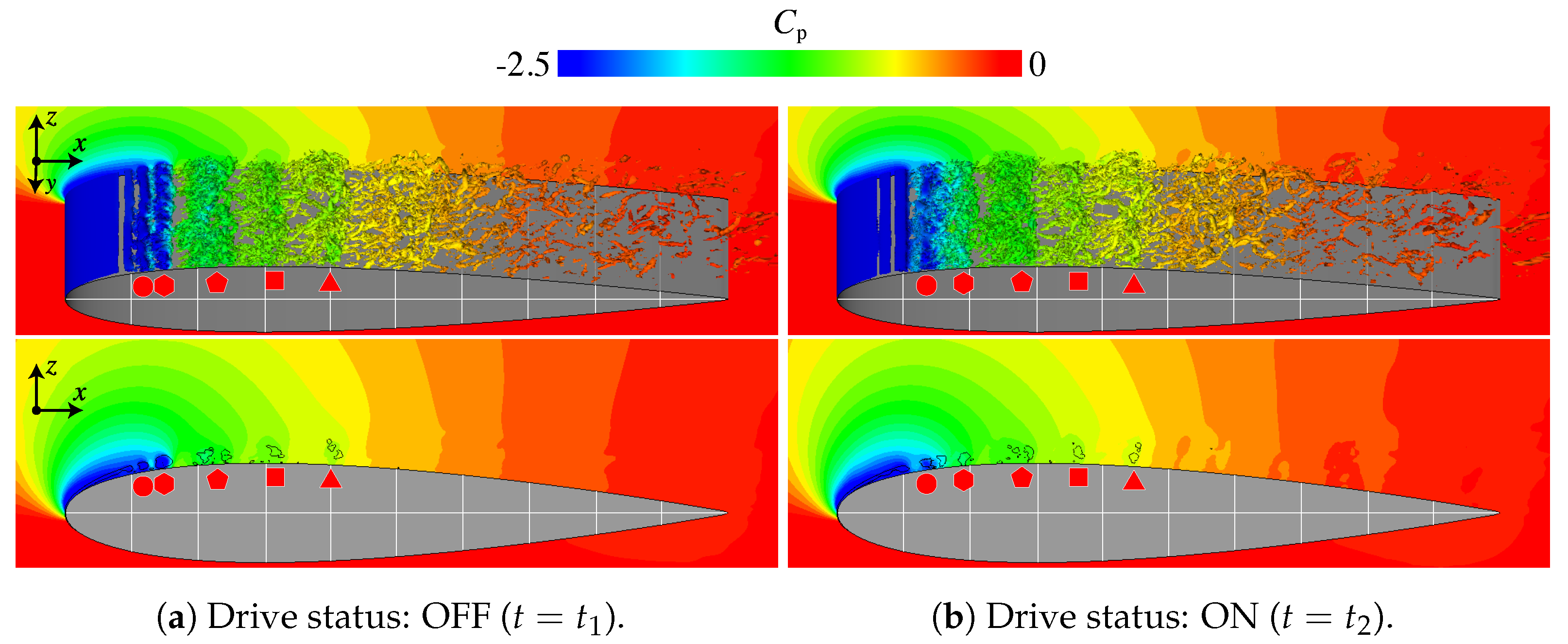
The flow field at $\alpha =12$ obtained by FTM1 was investigated to understand the flow control mechanism of the FTM. FTM1 is the case which has a modest control effect. Figure 9 shows the instantaneous flow fields of FTM1 at the characteristic flow states. Figure 9a shows the separated flow state at $t=t_1$. Figure 9b shows the attached flow state at $t=t_2$. The top figures show an overview of the instantaneous flows, and the bottom figures show the cross-sectional view of the spanwise-averaged flows. The isosurfaces in the top figures and the contour lines in the bottom figures are the second invariants of the velocity gradient tensor. The backgrounds and isosurfaces are colored based on $C_{\mathrm{p}}$. The symbols denote the locations of representative spanwise vortices. The background of the top figure is colored based on spanwise-averaged $C_{\mathrm{p}}$ over the upper surface of the airfoil. Figure 10 shows the time histories of $L/D$, $C_{\mathrm{p},\mathrm{var}}$ at the pressure sensor, and the drive status of the plasma actuator in FTM1 from the top to bottom. The top figure overlaps with the distribution of the spanwise-averaged $C_{\mathrm{p}}$ on the airfoil upper surface in the $x/c$-t domain. The plasma actuator in FTM1 is almost continuously driven and is rarely switched off, as shown in the bottom figure of Figure 10. However, although the flow of the continuous case remained in the separated flow, the FTM1 flow alternated between the separated flow states (Figure 9a) and the attached flow state (Figure 9b), unlike the continuous case. $L/D$ becomes low when the flow is separated ($t=t_1$) and high when the flow is attached ($t=t_2$), as shown in the top figure of Figure 10. In the attached flow state, several spanwise vortices are found on the airfoil surface (Figure 9b). Because a vortex forms a negative pressure region at the center of the vortex, its position and trajectory can be confirmed by observing the time variation of the surface pressure when the flow is attached. For example, around $x/c=0.4$ at the top of Figure 10, the trajectories of the vortices can be seen as numerous yellow stripes. In contrast, in the separated flow state ($15\lesssim t\lesssim 20$), the surface pressure is not disturbed because the vortices advect downstream away from the airfoil surface, and thus, $C_{\mathrm{p},\mathrm{var}}$ is relatively low. Thus, the plasma actuator is turned off when $C_{\mathrm{p},\mathrm{var}}$ falls below the threshold, but it is turned on again immediately in the case of FTM1. Such momentary turning off of the plasma actuator creates a strong vortex, as shown by the red dot in Figure 9, and the advection of that vortex causes the flow to be attached.

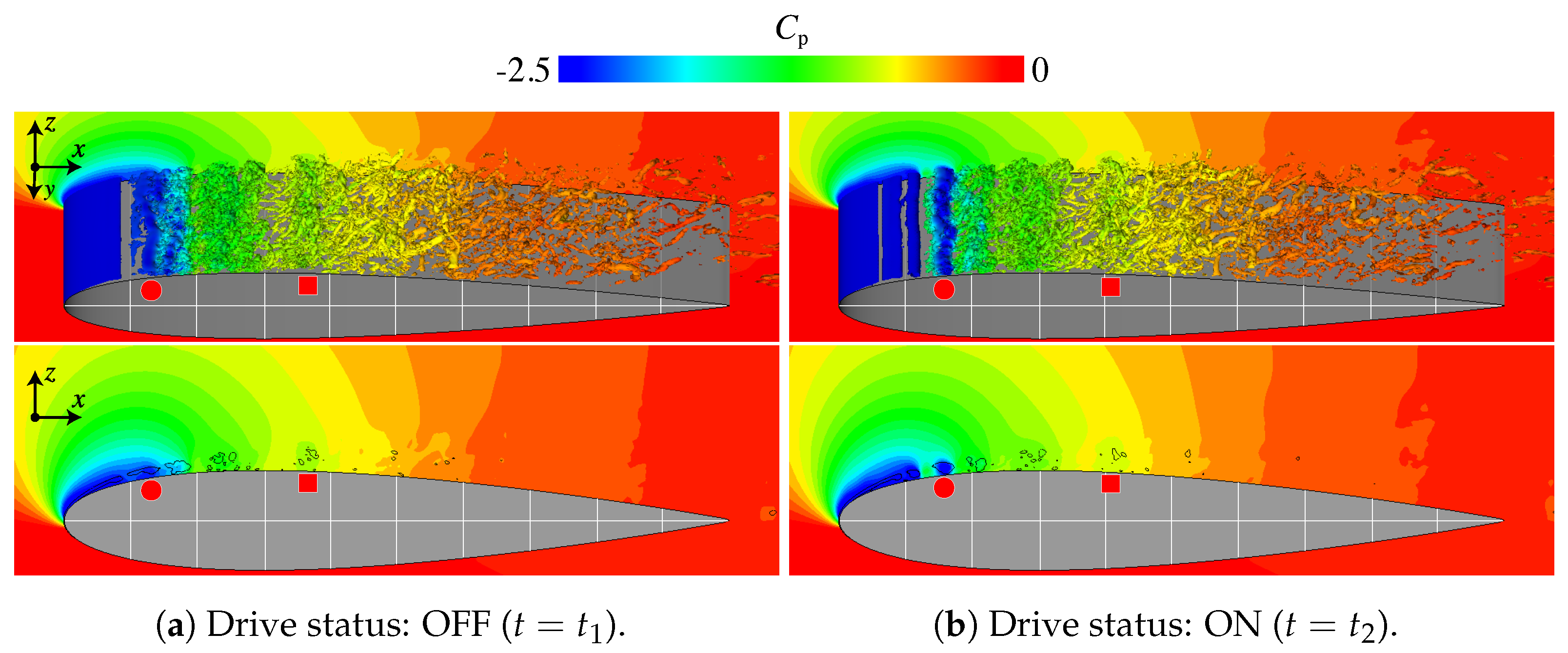
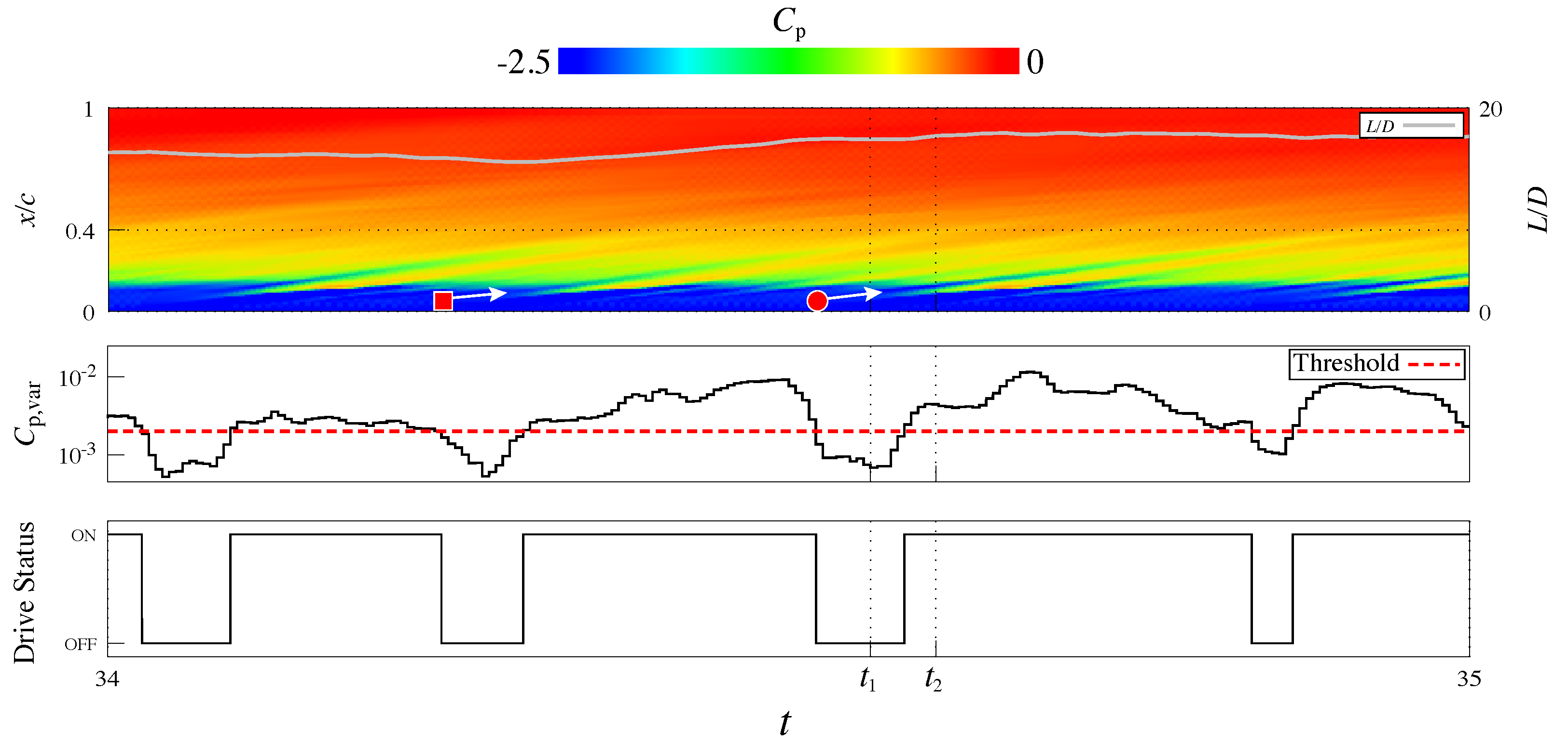
The flow of FTM4, which has the highest $L/D$ among the FTMs, is also discussed in Figure 11 and Figure 12. The isosurfaces and contour surfaces shown in Figure 11 are the same as those in Figure 9. Figure 11a shows the instantaneous flow fields when the plasma actuator is turned off. Figure 11b shows the instantaneous flow fields when the plasma actuator is turned on. The contour surface and the line plot in Figure 12 are the same as in Figure 10. The symbols and arrows in Figure 11 and Figure 12 represent the characteristic vortex positions and their trajectories, respectively. The flow of FTM4 attaches regardless of whether the plasma actuator is on or off (Figure 11), and $L/D$ maintains a high value (the top figure in Figure 12). The bottom of Figure 12 shows that the plasma actuator is intermittently driven, similar to classic burst actuation. The vortices generated near the leading edge by the plasma actuator coalesce into large vortices compared with FTM1. These vortices advect downstream and gradually collapse into fine three-dimensional vortices. The surface pressure stripes formed by the advection of the vortices are clearly observed at the position of $0.1\lesssim x/c\lesssim 0.5$. In particular, the vortices that shed near the leading edge when the plasma actuator is turned off were relatively strong, and their structures were maintained up to the vicinity of the pressure sensor. As they pass over the pressure sensor, $C_{\mathrm{p},\mathrm{var}}$ increases, and the plasma actuator turns on. Vortex generation according to the period of the plasma actuator being on and off is also found in the classic burst actuation case (Burst6). These results show that the FTM automatically becomes a pseudo-classic burst actuation by selecting an appropriate threshold.

4.4. Tendency of Drive Status of the FTM

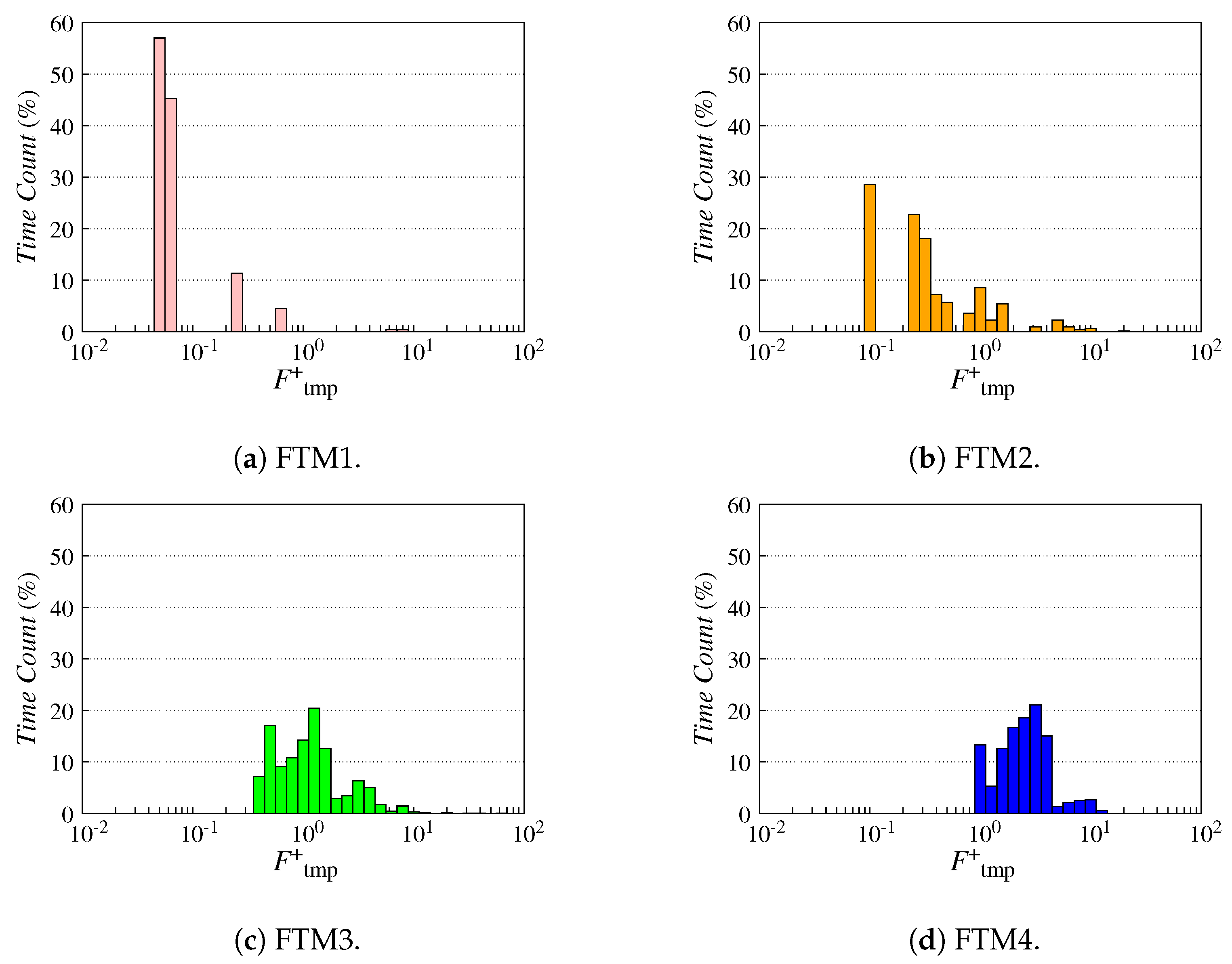
Figure 13 shows a histogram of $F_{\mathrm{tmp}}^{+}$ in each FTM case. The horizontal axis is the log scale. From FTM1 to FTM4, the overall distribution of $F_{\mathrm{tmp}}^{+}$ shifts to a higher value as the threshold value increases. In FTM1, the plasma actuator is driven almost continuously and rarely turns off. Thus, $F_{\mathrm{tmp}}^{+}$ is mainly distributed at low values. The frequency appearing most frequently is $F_{\mathrm{tmp}}^{+}\simeq 0.6$, which is equivalent to the frequency at which the flow alternates between the separated and attached states. FTM4 is driven almost similar to classic burst actuation, and $F_{\mathrm{tmp}}^{+}$ is found in $1\lesssim F_{\mathrm{tmp}}^{+}\lesssim 10$. The frequency of $F_{\mathrm{tmp}}^{+}\lesssim 1$ was not found for FTM4. The obtained frequency band of $F_{\mathrm{tmp}}^{+}$ in FTM4 is based on the advection periods of the vortices generated by the drive of the plasma actuator and corresponds to the frequency band which is effective for separation flow control, which has been clarified in previous studies [23,27].

$F_{\mathrm{tmp}}^{+}$ in the FTM can be automatically modulated in the frequency band, where the plasma actuator can maintain the attached flow by setting an appropriate threshold value. However, an appropriate threshold value must be determined in advance. Therefore, based on the knowledge obtained from the FTM results, we propose and investigate an improved control method that does not require a threshold setting in Section 5.

5. Dynamic Threshold Method (DTM)

The DTM is introduced as a novel dynamic burst actuation method based on the findings of the FTM in Section 4. First, the effectiveness and control mechanism of the DTM at $\alpha =12$ are discussed and compared with those of the FTM. Second, the LES results at $\alpha =16$ are discussed to evaluate the adaptability of the DTM.

5.1. Introduction of the DTM

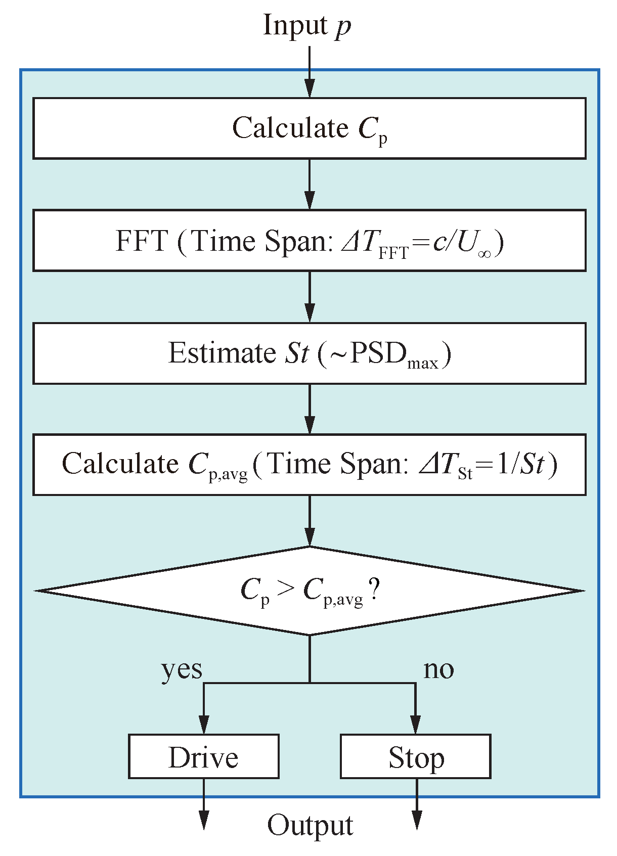
Figure 14 shows the DTM control flowchart. The controller receives instantaneous pressure from a single pressure sensor and stores its time-series data, similar to the FTM. In the controller, the moving average ($C_{\mathrm{p},\mathrm{avg}}$) of the pressure coefficient is calculated from the acquired data through the following equations:

$$\begin{array}{cc}\hfill C_{\mathrm{p},\mathrm{avg}}\left(t_n\right)& =\frac{1}{N}\sum _{i=1}^N{C}_{\mathrm{p}}\left(t_i\right)\left(t_n\ge \Delta T_{\mathrm{FFT}}\right),\hfill \end{array}$$

(17)

$$\begin{array}{cc}\hfill C_{\mathrm{p}}\left(t_i\right)& ={\displaystyle \frac{p\left(t_i\right)-p_{\infty }}{{\displaystyle \frac{1}{2}}\rho {U_{\infty }}^2}},\hfill \end{array}$$

(18)

$$\begin{array}{cc}\hfill t_i& =(n-N+i)\Delta t_{\mathrm{sens}},\hfill \end{array}$$

(19)

$$\begin{array}{cc}\hfill N& ={\displaystyle \frac{\Delta T_{St}\left(t_n\right)}{\Delta t_{\mathrm{sens}}}}+1,\hfill \end{array}$$

(20)

where $\Delta T_{St}$ is a time scale obtained from the frequency $St$, which is dominant in the time fluctuations of $C_{\mathrm{p}}$ and $\Delta T_{St}=1/St$. $St$ is obtained by a short-time fast Fourier transform (FFT) for the acquired pressure time-series data. The time duration ($\Delta T_{\mathrm{FFT}}$) for acquiring the data used for the short-time FFT is unity in non-dimensional time to cover the frequency bands that were effective in the FTM and Burst6. The obtained $C_{\mathrm{p},\mathrm{avg}}$ is compared with $C_{\mathrm{p}}$ at that time, when $C_{\mathrm{p}}$ is higher than $C_{\mathrm{p},\mathrm{avg}}$, PA is driven, and when $C_{\mathrm{p}}$ is lower, PA is stopped. In other words, the DTM is a method in which $C_{\mathrm{p},\mathrm{var}}$ and fixed thresholds of the FTM are replaced with $C_{\mathrm{p}}$ and $C_{\mathrm{p},\mathrm{avg}}$, respectively.

5.2. Comparison of DTM and FTM

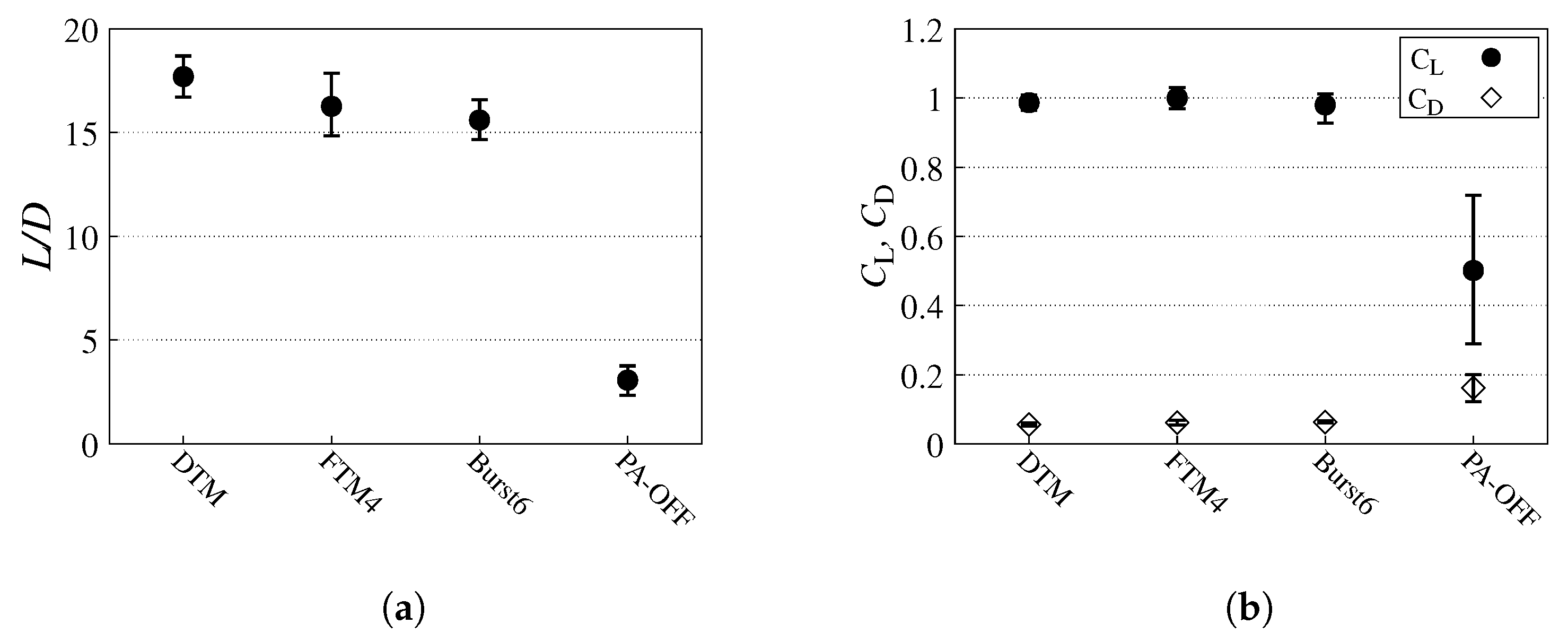
Figure 15 shows $L/D$, $C_{\mathrm{L}}$, and $C_{\mathrm{D}}$ at $\alpha =12$ in the DTM, FTM4, and the previous computational results (Burst6 and PA-OFF) [24] at $\alpha =12$. Burst6 is the classic burst actuation case with a burst frequency of $F^{+}=6$, which is the effective burst frequency for flow separation control at $\alpha =12$. The burst ratio is $0.1$. PA-OFF is the case without the control of the plasma actuator. The symbols and error bars are the same as those in Figure 8. Figure 15 shows that the DTM has the highest $L/D$ in the cases considered. The mean value of $L/D$ is 1.08 times larger than that of FTM4, and the fluctuation of $L/D$ is also smaller than that of FTM4. Additionally, the minimum $L/D$ value of the DTM is higher than the maximum $L/D$ value of Burst6. The reduction in $C_{\mathrm{D}}$ mainly contributes to the $L/D$ improvement of the DTM. Although the mean value of $C_{\mathrm{L}}$ is slightly lower than that of FTM4, the fluctuation is smaller than that of FTM4 and Burst6. In the FTM and classic burst actuation, the parameters (i.e., the fixed threshold value and the burst frequency) that strongly affect the flow control effect must be determined in advance. However, the DTM can obtain a control effect without predetermining these parameters.

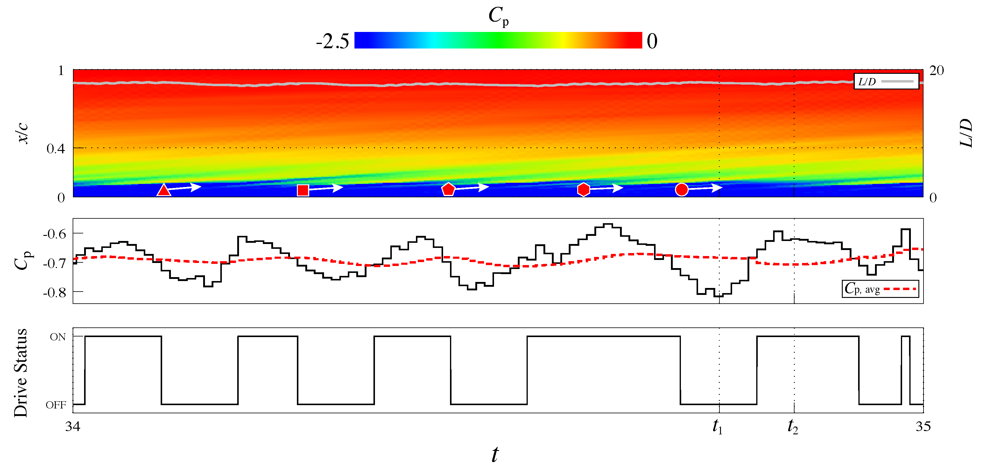
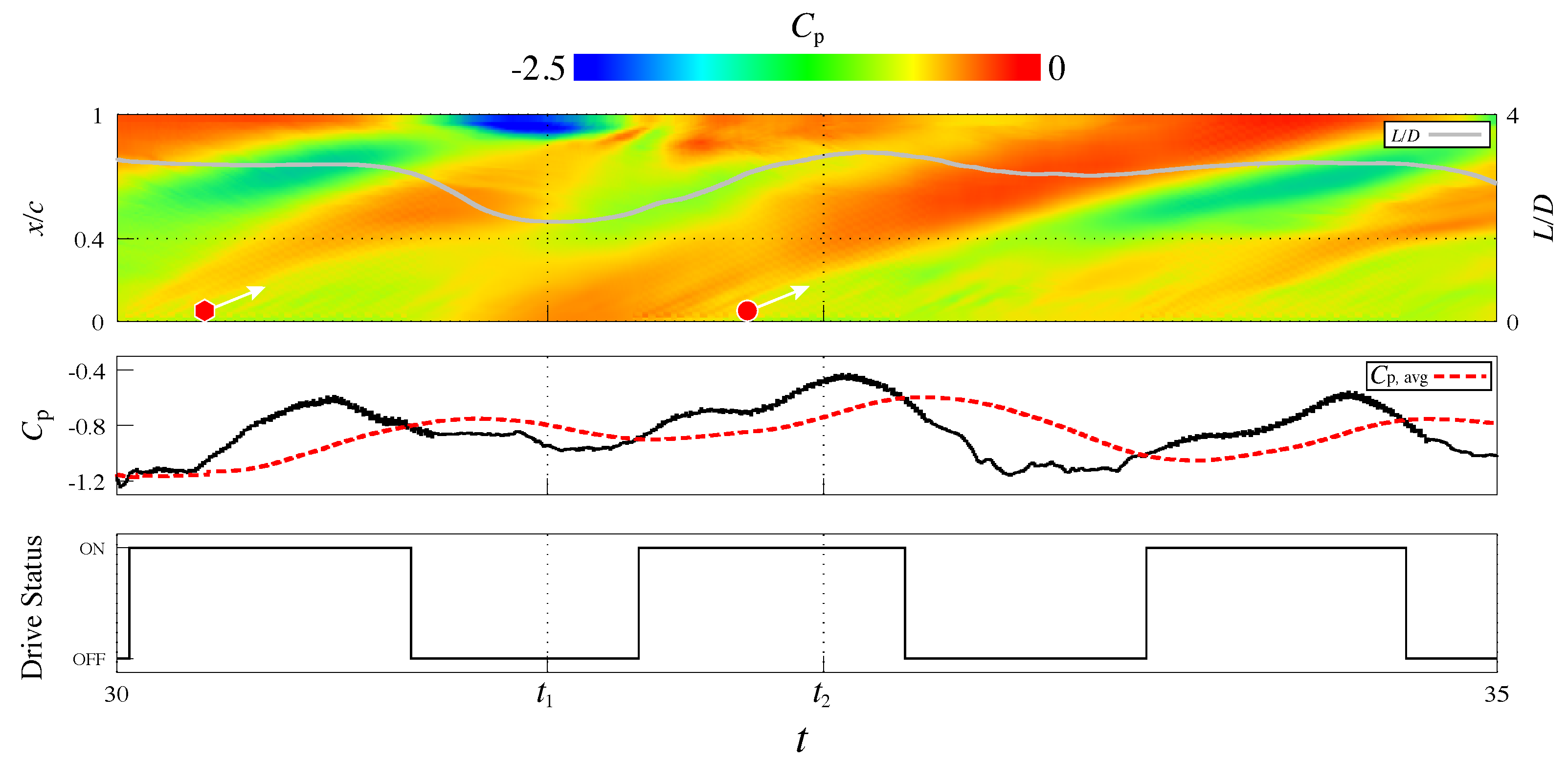
The flow fields of the DTM at $\alpha =12$ and the related graphs are discussed to understand the flow control mechanism. Figure 16 shows that the instantaneous flow fields of the DTM and the isosurfaces and the contour surfaces are the same as in Figure 9. Figure 17 shows the time histories of $L/D$ and $C_{\mathrm{p}}$, and the driving state of the plasma actuator from the top to bottom. The top figure overlaps with the distribution of the spanwise-averaged $C_{\mathrm{p}}$ on the upper surface of the airfoil in the $x/c$-t domain. As shown in Figure 16, the flow attaches without massive separation regardless of whether the plasma actuator is on or off. Moreover, because the flow is stably attached, $C_{\mathrm{L}}$ maintains a high value, as shown in the top figure of Figure 17, and there is no large fluctuation in $C_{\mathrm{L}}$. $C_{\mathrm{p}}$ fluctuates each time the vortices generated by the drive of the plasma actuator pass over the pressure sensor. In contrast, although $C_{\mathrm{p},\mathrm{avg}}$ is a moving average value, it is almost constant because the flow is quasi-stationary. Similar to FTM4, the drive of the plasma actuator in the DTM turns on and off almost periodically (Figure 17, bottom figure). The on and off states of the plasma actuators are switched each time the spanwise vortex passes through the pressure sensor. The spanwise vortices generated by the drive of the plasma actuator in the DTM maintain their structures until they pass over the pressure sensor compared to FTM4. In addition, in the DTM, the on- and off-switching cycles are shorter, and the distance between the vortices generated by driving the plasma actuator is narrower than that of FTM4.

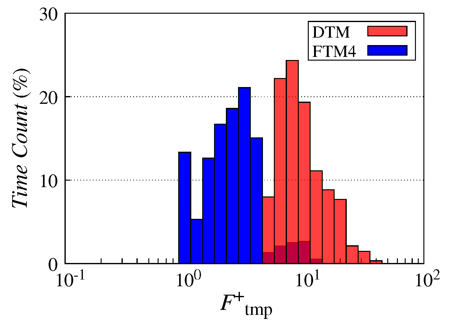
Figure 18 shows a histogram of $F_{\mathrm{tmp}}^{+}$ for the DTM and FTM4 at $\alpha =12$. The horizontal axis is the log scale. In FTM4, $F_{\mathrm{tmp}}^{+}\simeq 4$ appears the most often, and $F_{\mathrm{tmp}}^{+}$ is distributed in $1\lesssim F_{\mathrm{tmp}}^{+}\lesssim 10$. In the DTM, $F_{\mathrm{tmp}}^{+}$ is distributed in $6\lesssim F_{\mathrm{tmp}}^{+}\lesssim 30$, and $F_{\mathrm{tmp}}^{+}\simeq 10$ appears most often. Overall, $F_{\mathrm{tmp}}^{+}$ of the DTM is higher than that of FTM4. This result is consistent with the fact that the interval between the vortices passing over the pressure sensor in the DTM is shorter, and the switching interval between the on and off states of the plasma actuator is shorter in FTM4. Previous studies have clarified that a burst frequency of $F^{+}=6$ (Burst6) is effective for flow separation control under the present flow conditions [23,27]. In the present study, using the DTM, we were able to automatically find the $F_{\mathrm{tmp}}^{+}$ frequency band, which includes the effective frequency ($F^{+}=6$) for the flow separation control and is even more effective, without using a fixed threshold value.

5.3. Robustness of DTM

In the classic burst actuation control, the effective burst frequency $F^{+}$ for flow separation control must be identified in advance, and the effective $F^{+}$ differs depending on the flow conditions. At a shallow post-stall angle ($\alpha =12$), the burst actuation of $F^{+}\simeq 10$ effectively suppresses the flow separation and improves the $L/D$. In contrast, at a deeper angle of attack or a higher Reynolds number, $F^{+}\simeq 10$ is less effective for separation control. Under such conditions, $F^{+}\simeq 1$ is effective, and $C_{\mathrm{L}}$ slightly increases using $F^{+}\simeq 1$ [23,27]. In this section, we perform the LES of the flow controlled by the DTM at $\alpha =16$ and evaluate the robustness of the DTM.

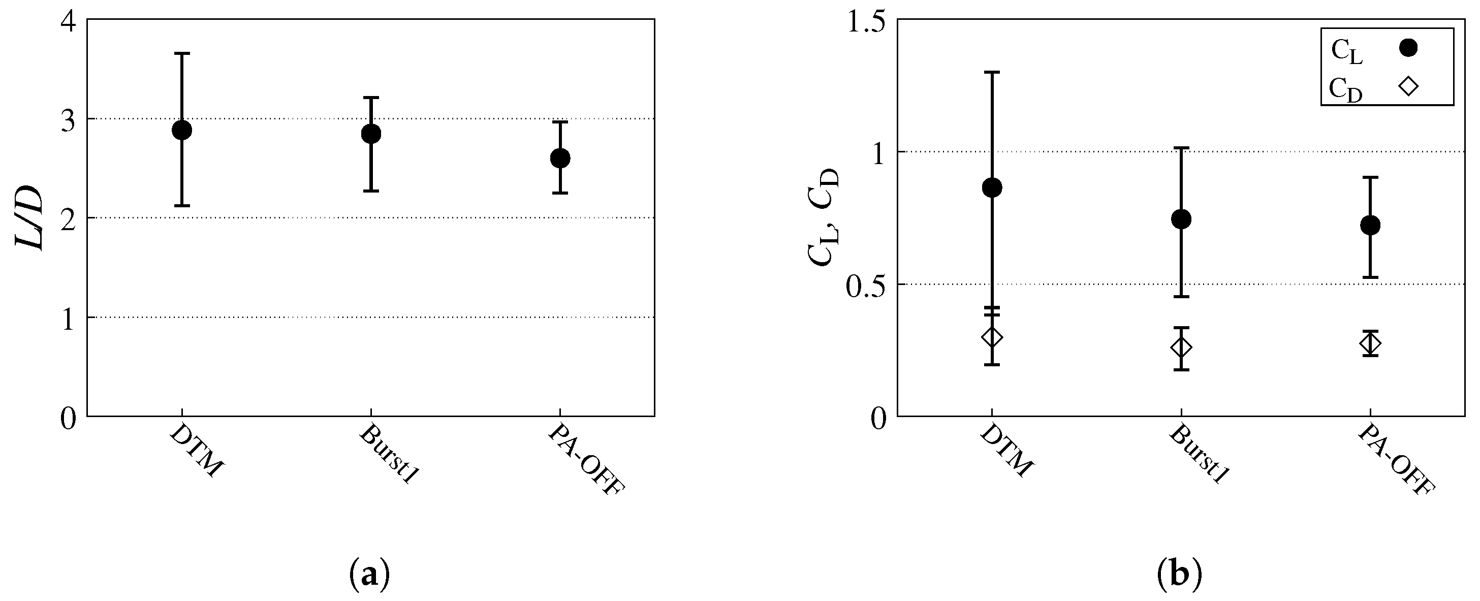
Figure 19 shows the $L/D$, $C_{\mathrm{L}}$, and $C_{\mathrm{D}}$ of the DTM result at $\alpha =16$ and those of the previous computational results (Burst1 and PA-OFF) [24]. Burst1 is the classic burst actuation case using $F^{+}=1$ with $BR=0.1$, which is effective for separation control at $\alpha =16$. PA-OFF is the case without control of the plasma actuator at $\alpha =16$. Although the fluctuation of $L/D$ is larger, the DTM provides a higher mean $L/D$ and $C_{\mathrm{L}}$ than the classic burst actuation case (Burst1). The mean value of $L/D$ is 1.02 times that of Burst1. The lift increase contributes to the improvement in $L/D$. The mean value of $C_{\mathrm{L}}$ is 1.13 times that of Burst1.

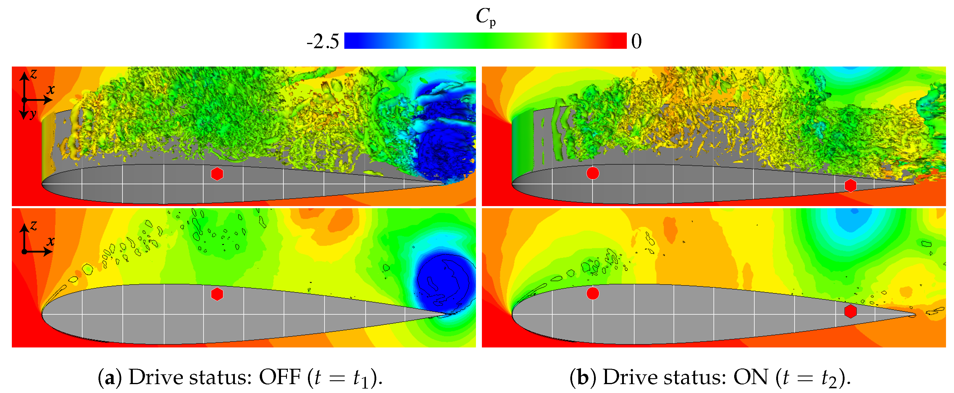
The relationship between the flow fields and the driving state of the plasma actuator of the DTM at $\alpha =16$ is discussed in Figure 20 and Figure 21. The isosurfaces and contour surfaces shown in Figure 20 are the same as those shown in Figure 9, and the contour surfaces and lines in Figure 21 are the same as in Figure 17. As shown in Figure 20, the flow separation is not completely suppressed, and large-scale vortex structures can be seen on the upper surface of the airfoil surface. The red symbols indicate the chordwise positions of the vortices in Figure 20. These large vortices are yielded by the coalescence of several vortices generated by the drive of the plasma actuator. The plasma actuator periodically repeats on and off, similar to classic burst actuation (Figure 21, bottom figure) as in the case of $\alpha =12$ (Figure 17). The period during which the plasma actuator switches on and off and the period of a large vortex passing over the airfoil surface are approximately the same. The present flow field obtained by the DTM is similar to that obtained by $F^{+}=1$ of the classic burst actuation control (Burst1) [25]. In addition, owing to the advection of the vortices, the pressure on the airfoil surface fluctuates periodically, and $C_{\mathrm{L}}$ also fluctuates significantly (Figure 21, top figure). $C_{\mathrm{p}}$ on the pressure sensor also takes a low value each time the vortex passes, and the drive state of the plasma actuator also switches on and off according to the passage of the vortex (Figure 21, bottom figure).

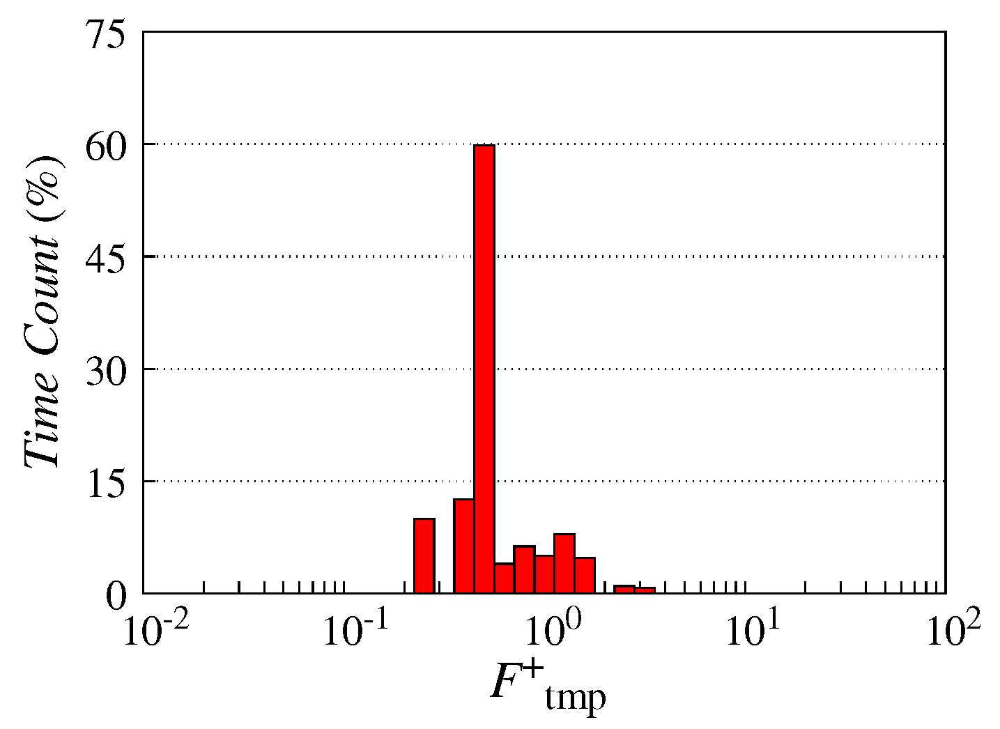
Figure 22 shows a histogram of the DTM’s $F_{\mathrm{tmp}}^{+}$ at $\alpha =16$. The horizontal axis of Figure 22 is the log scale. $F_{\mathrm{tmp}}^{+}$ takes a value between 0.3 and 3. $F_{\mathrm{tmp}}^{+}=0.5$ appears the most often. This frequency band is lower than that in the DTM at $\alpha =12$ and contains $F^{+}\simeq 1$, which is known as the burst frequency effective for flow separation control at a deep stall angle [23,27]. The DTM automatically selects the effective drive state of the plasma actuator for flow separation control according to the flow condition, even at $\alpha =16$, and improves the $L/D$ owing to the increase in $C_{\mathrm{L}}$.

6. Conclusions

In this study, we propose dynamic burst actuation of plasma actuators to enhance their flow control authority. To verify the effectiveness of this approach, three-dimensional compressible Navier–Stokes equations with the DBD plasma actuator body force terms were solved by implicit large-eddy simulations (iLES). The plasma actuator was installed at the 5% chord position from the leading edge of a cross-section of an NACA0015 airfoil. A single-point pressure sensor was installed at the 40% chord position in the middle of the airfoil span, and the separated flows were controlled by the DBD plasma actuator, where the AC voltage was modulated with the duty cycle not given a priori but dynamically changed based on the measured pressure fluctuations given by the point sensor. Simulations under post-stall angles of attack of 12° or 16° were carried out at a Reynolds number of 63,000.

Two modulation strategies were considered, and their results were discussed. When the DBD plasma actuator was turned on and off in time simply based on the pressure fluctuation values being above or below the given threshold, good flow control authority was observed in general. The flow control authority improved when the threshold value was appropriately chosen, and a fixed burst frequency that was proven to be effective by the former studies was automatically realized. When the measured $C_{\mathrm{p}}$ moving average in time was used as a threshold, better flow control authority was realized. In this approach, the threshold was automatically determined and did not have to be given in advance. Application to the case at a higher angle of attack showed the robustness of the second approach. In general, a simple feedback loop using single-point pressure data over the airfoil surface was shown to be effective as a robust flow control method and solved the problem of difficulty in choosing the appropriate burst frequencies depending on the airfoil geometry and flow conditions.

References

- Roth, J.R.; Sherman, D.M.; Wilkinson, S.P. Electro hydrodynamic Flow Control with a Glow-Discharge Surface Plasma. AIAA J. 2000, 38, 1166–1172. [Google Scholar] [CrossRef]
- Post, M.L.; Corke, T.C. Separation Control on High Angle of Attack Airfoil Using Plasma Actuators. AIAA J. 2004, 42, 2177–2184. [Google Scholar] [CrossRef]
- Post, M.L.; Corke, T.C. Separation Control Using Plasma Actuators: Dynamic Stall Vortex Control on Oscillating Airfoil. AIAA J. 2006, 44, 3125–3135. [Google Scholar] [CrossRef]
- Greenblatt, D.; Goksel, B.; Schule, C.Y.; Romann, D.; Paschereit, C.O. Dielectric Barrier Discharge Flow Control at Very Low Flight Reynolds Numbers. AIAA J. 2008, 46, 1528–1541. [Google Scholar] [CrossRef]
- Bénard, N.; Jolibois, J.; Moreau, E. Lift and drag performances of an axisymmetric airfoil controlled by plasma actuator. J. Electrost. 2009, 67, 133–139. [Google Scholar] [CrossRef]
- Greenblatt, D.; Schneider, T.; Schuele, C.Y. Mechanism of flow separation control using plasma actuation. Phys. Fluids 2012, 24, 077102. [Google Scholar] [CrossRef]
- Little, J.; Nishihara, M.; Adamovich, I.; Samimy, M. High-lift airfoil trailing edge separation control using a single dielectric barrier discharge plasma actuator. Exp. Fluids 2010, 48, 521–537. [Google Scholar] [CrossRef]
- Little, J.; Takashima, K.; Nishihara, M.; Adamovich, I.; Samimy, M. Separation Control with Nanosecond-Pulse-Driven Dielectric Barrier Discharge Plasma Actuators. AIAA J. 2012, 50, 350–365. [Google Scholar] [CrossRef]
- Visbal, M.R. Strategies for control of transitional and turbulent flows using plasma-based actuators. Int. J. Comput. Fluid Dyn. 2010, 24, 237–258. [Google Scholar] [CrossRef]
- Gaitonde, D.V. Analysis of plasma-based flow control mechanisms through large-eddy simulations. Comput. Fluids 2013, 85, 19–26. [Google Scholar] [CrossRef]
- Asada, K.; Nonomura, T.; Aono, H.; Sato, M.; Okada, K.; Fujii, K. LES of transient flows controlled by DBD plasma actuator over a stalled airfoil. Int. J. Comput. Fluid Dyn. 2015, 29, 215–229. [Google Scholar] [CrossRef]
- Segawa, T.; Suzuki, D.; Fujino, T.; Jukes, T.; Matsunuma, T. Feedback Control of Flow Separation Using Plasma Actuator and FBG Sensor. Int. J. Aerosp. Eng. 2016, 2016, 8648919. [Google Scholar] [CrossRef] [Green Version]
- Wu, B.; Gao, C.; Liu, F.; Xue, M.; Zheng, B. Simulation of NACA0015 flow separation controlby burst-mode plasma actuation. Phys. Plasmas 2019, 26, 063507. [Google Scholar] [CrossRef]
- Abe, T.; Asada, K.; Sekimoto, S.; Fukudome, K.; Tatsukawa, T.; Mamori, H.; Fujii, K.; Yamamoto, M. Computational Study of Wing-Tip Effect for Flow-Control Authority of Dielectric-Barrier-Discharge Plasma Actuator. AIAA J. 2021, 59, 104–117. [Google Scholar] [CrossRef]
- Borghi, C.A.; Cristofolini, A.; Neretti, G.; Seri, P.; Rossetti, A.; Talamelli, A. Duty cycle and directional jet effects of a plasma actuator on the flow control around a NACA0015 airfoil. Meccanica 2017, 52, 3661–3674. [Google Scholar] [CrossRef]
- Zoppini, G.; Belan, M.; Zanotti, A.; Vinci, L.D.; Campanardi, G. Stall Control by Plasma Actuators: Characterization along the Airfoil Span. Energies 2020, 13, 1374. [Google Scholar] [CrossRef] [Green Version]
- Mahdavi, H.; Daliri, A.; Sohbatzadeh, F.; Shirzadi, M.; Rezanejad, M. A single unsteady DBD plasma actuator excitedby applying two high voltages simultaneouslyfor flow control. Phys. Plasmas 2020, 27, 083514. [Google Scholar] [CrossRef]
- Shimomura, S.; Sekimoto, S.; Oyama, A.; Fujii, K.; Nishida, H. Closed-Loop Flow Separation Control Using the Deep Q Network over Airfoil. AIAA J. 2020, 58, 4260–4270. [Google Scholar] [CrossRef]
- Sekimoto, S.; Fujii, K.; Hosokawa, S.; Akamatsu, H. Flow-control capability of electronic-substrate-sized power supply for a plasma actuator. Sens. Actuators A Phys. 2020, 306, 111951. [Google Scholar] [CrossRef]
- Corke, T.; Post, M.; Orlov, D. Single dielectric barrier discharge plasma enhanced aerodynamics: Physics, modeling and applications. Exp. Fluids 2009, 46, 1–26. [Google Scholar] [CrossRef]
- Fujii, K. High-performance computing-based exploration of flow control with micro devices. Philos. Trans. R. Soc. A 2014, 372, 20130326. [Google Scholar] [CrossRef] [Green Version]
- Asada, K.; Ninomiya, Y.; Oyama, A.; Fujii, K. Airfoil Flow Experiment on the Duty Cycle of DBD Plasma Actuator. In Proceedings of the 47th AIAA Aerospace Sciences Meeting including The New Horizons Forum and Aerospace Exposition, Orlando, FL, USA, 5–8 January 2009. [Google Scholar] [CrossRef]
- Sekimoto, S.; Nonomura, T.; Fujii, K. Burst-Mode Frequency Effects of Dielectric Barrier Discharge Plasma Actuator for Separation Control. AIAA J. 2017, 55, 1385–1392. [Google Scholar] [CrossRef]
- Sato, M.; Aono, H.; Yakeno, A.; Nonomura, T.; Fujii, K.; Okada, K.; Asada, K. Multifactorial Effects of Operating Conditions of Dielectric-Barrier-Discharge Plasma Actuator on Laminar-Separated-Flow Control. AIAA J. 2015, 53, 2544–2559. [Google Scholar] [CrossRef]
- Sato, M.; Nonomura, T.; Okada, K.; Asada, K.; Aono, H.; Yakeno, A.; Abe, Y.; Fujii, K. Mechanisms for laminar separated-flow control using dielectric-barrier-discharge plasma actuator at low Reynolds number. Phys. Fluids 2015, 27, 117101. [Google Scholar] [CrossRef]
- Fujii, K. Three Flow Feature behind the Flow Control Authority of DBD Plasma Actuator: Result of High-Fidelity Simulations and the Related Experiments. Appl. Sci. 2018, 8, 546. [Google Scholar] [CrossRef] [Green Version]
- Sato, M.; Okada, K.; Asada, K.; Aono, H.; Nonomura, T.; Fujii, K. Unified mechanisms for separation control around airfoil using plasma actuator with burst actuation over Reynolds number range of 103–106. Phys. Fluids 2020, 32, 025102. [Google Scholar]
- Benard, N.; III, L.N.C.; Moreau, E.; Griffin, J.; Bonnet, J. On the Benefits of Hysteresis Effects for Closed-Loop Separation Control Using Plasma Actuation. Phys. Fluids 2011, 23, 083601. [Google Scholar] [CrossRef]
- Ogawa, T.; Shimomura, S.; Asada, K.; Sekimoto, S.; Tatsukawa, T.; Nishida, H.; Fujii, K. Study on the Sensing Parameters toward Better Feed-back Control of Stall Separation with DBD Plasma Actuator. In Proceedings of the 35th AIAA Applied Aerodynamics Conference, Denver, CO, USA, 5–9 June 2017. [Google Scholar]
- Ogawa, T.; Asada, K.; Sekimoto, S.; Tatsukawa, T.; Fujii, K. Feed-back Control of Stall Separation with DBD Plasma Actuator by Detecting Vortex Passing over an Airfoil. In Proceedings of the 2018 AIAA Aerospace Sciences Meeting, Kissimmee, FL, USA, 8–12 January 2018. [Google Scholar]
- Suzen, Y.B.; Huang, P.G. Simulations of Flow Separation Contorl using Plasma Actuator. In Proceedings of the 44th AIAA Aerospace Sciences Meeting and Exhibit, Reno, NV, USA, 9–12 January 2006. [Google Scholar]
- Aono, H.; Sekimoto, S.; Sato, M.; Yakeno, A.; Nonomura, T.; Fujii, K. Computational and experimental analysis of flow structures induced by a plasma actuator with burst modulations in quiescent air. Mech. Eng. J. 2015, 2, 15-00233. [Google Scholar] [CrossRef] [Green Version]
- Font, G.I.; Enloe, C.L.; McLaughlin, T.E. Plasma Volumetric Effects on the Force Production of a Plasma Actuator. AIAA J. 2010, 48, 1869–1874. [Google Scholar] [CrossRef]
- Chen, D.; Asada, K.; Sekimoto, S.; Fujii, K.; Nishida, H. A high-fidelity body-force modeling approachfor plasma-based flow control simulations. Phys. Fluids 2021, 33, 037115. [Google Scholar] [CrossRef]
- Kawai, S.; Fujii, K. Analysis and Prediction of Thin-Airfoil Stall Phenomena Using Hybrid Turbulent Methodology. AIAA J. 2005, 43, 953–961. [Google Scholar] [CrossRef]
- Kojima, R.; Nonomura, T.; Oyama, A.; Fujii, K. Large-Eddy Simulation of Low-Reynolds-Number Flow Over Thick and Thin NACA Airfoils. J. Aircr. 2013, 50, 187–196. [Google Scholar] [CrossRef]
- Lee, D.; Kawai, S.; Nonomura, T.; Anyoji, M.; Aono, H.; Oyama, A.; Asai, K.; Fujii, K. Mechanisms of surface pressure distribution within a laminar separation bubble at different Reynolds numbers. Phys. Fluids 2015, 27, 023602. [Google Scholar] [CrossRef]
- Lele, S.K. Compact Finite Difference Schemes with Spectral-like Resolution. J. Comput. Phys. 1992, 103, 16–42. [Google Scholar] [CrossRef]
- Gaitonde, D.V.; Visbal, M.R. Padé-Type Higher-Order Boundary Filters for the Navier-Stokes Equations. AIAA J. 2000, 38, 2103–2112. [Google Scholar] [CrossRef]
- Visbal, M.R.; Rizzetta, D.P. Large-Eddy Simulation on Curvilinear Grids Using Compact Differencing and Filtering Schemes. J. Fluids Eng. 2002, 124, 836–847. [Google Scholar] [CrossRef]
- Fujii, K. Simple Ideas for the Accuracy and Efficiency Improvement of the Compressible Flow Simulation Methods. In Proceedings of the International CFD Workshop on Supersonic Transport Design, Tokyo, Japan, 16–17 March 1998; pp. 20–23. [Google Scholar]
- Choi, H.; Moin, P. Effects of the Computational Time Step on Numerical Solutions of Turbulent Flow. J. Comput. Phys. 1994, 113, 1–4. [Google Scholar] [CrossRef]
- Fujii, K. Unified Zonal Method Based on the Fortified Solution Algorithm. J. Comput. Phys. 1995, 118, 92–108. [Google Scholar] [CrossRef]
Figure 1.
Schematic diagram of the DBD plasma actuator and an example of the practical application.
Figure 2.
Waveform for burst actuation.
Figure 3.
Schematic of the dynamic burst actuation.
Figure 4.
Waveform for the dynamic burst actuation.
Figure 5.
Distribution of body force in the x direction based on the Suzen–Huang model [31] and body force vectors near the actuator. Gray and orange areas represent the airfoil surface and exposed electrode, respectively.
Figure 6.
Computational grids and computational domain. The grids were visualized for every four points. (a) Perspective view. (b) Cross-sectional view. (c) Computational domain.
Figure 7.
Control flowchart of FTM.
Figure 8.
Aerodynamic characteristics in each FTM and reference cases at . (a) Lift-to-drag ratio (). (b) Lift and drag coefficients ( and ).
Figure 9.
Instantaneous flow field (top, ) and spanwise-averaged flow field (bottom, ) with isosurfaces of the second invariant of the velocity gradient tensor (Q) colored based on the pressure coefficient () in FTM1 at . The red circles denote the locations of representative spanwise vortices.
Figure 10.
Time histories of , at the pressure sensor and the drive status of the plasma actuator in FTM1 from top to bottom. The top figure overlaps with the distribution of the spanwise-averaged on the upper surface of the airfoil in the -t domain.
Figure 11.
Instantaneous flow field (top, ) and spanwise-averaged flow field (bottom, ) with isosurfaces of the second invariant of the velocity gradient tensor (Q) colored based on in FTM4 at . The red circles and squares denote the locations of representative spanwise vortices.
Figure 12.
The time histories of , at the pressure sensor and the drive status of the plasma actuator in FTM4 from the top to bottom. The top figure overlaps with the distribution of the spanwise-averaged on the upper surface of the airfoil in the -t domain. The red symbols and arrows represent the characteristic vortex positions and their trajectories.
Figure 13.
Temporary burst frequency () histogram in each FTM case at .
Figure 14.
Control flowchart of the DTM.
Figure 15.
Aerodynamic characteristics in the DTM, FTM4, and the reference cases at . (a) Lift- to-drag ratio (). (b) Lift and drag coefficients ( and ).
Figure 16.
Instantaneous flow field (top, ) and spanwise-averaged flow field (bottom, ) with isosurfaces of the second invariant of the velocity gradient tensor (Q) colored based on in the DTM at . The red symbols denote the locations of representative spanwise vortices.
Figure 17.
Time histories of , at the pressure sensor, and the drive status of the plasma actuator in FTM1 from the top to bottom. The top figure overlaps with the distribution of the spanwise-averaged on the upper surface of the airfoil in the -t domain. The red symbols and arrows represent the characteristic vortex positions and their trajectories.
Figure 18.
Temporary burst frequency () histograms in the DTM and FTM4 at .
Figure 19.
Aerodynamic characteristics in the DTM and the reference cases at . (a) Lift- to-drag ratio (). (b) Lift and drag coefficients ( and ).
Figure 20.
Figure 21.
The time histories of , at the pressure sensor and the drive status of the plasma actuator in FTM4 from top to bottom. The top figure overlaps with the distribution of the spanwise-averaged on the upper surface of the airfoil in the -t domain. The red symbols and arrows represent the characteristic vortex positions and their trajectories.
Figure 22.
Temporary burst frequency () histogram in the DTM at .