Analysis of Kinematics of Flapping Wing UAV Using OptiTrack Systems

Abstract

An analysis of the kinematics of a flapping membrane wing using experimental kinematic data is presented. This motion capture technique tracks the positon of the retroreflective marker(s) placed on the left wing of a 1.3-m-wingspan ornithopter. The time-varying three-dimensional data of the wing kinematics were recorded for a single frequency. The wing shape data was then plotted on a two-dimensional plane to understand the wing dynamic behaviour of an ornithopter. Specifically, the wing tip path, leading edge bending, wing membrane shape, local twist, stroke angle and wing velocity were analyzed. As the three characteristic angles can be expressed in the Fourier series as a function of time, the kinematics of the wing can be computationally generated for the aerodynamic study of flapping flight through the Fourier coefficients presented. Analysis of the ornithopter wing showed how the ornithopter closely mimics the flight motions of birds despite several physical limitations.

1. Introduction

Flapping wing flight is one of the most successful and widely used forms of locomotion in the natural world. Approximately 10 thousand scientifically described species of birds and nearly a million known insects rely on powered flight as a form of aerial locomotion [1]. Unlike conventional aerial vehicles which rely on a rigid wing and propeller to generate lift and thrust respectively, or a rotary wing in the case of a rotorcraft to generate both lift and thrust, birds generate lift and thrust by moving their wings relative to their body in an oscillatory (flapping) motion.

Aerial vehicles that imitate this oscillatory motion for the purpose of flight are known as ornithopters. Ornithopters offer several potential advantageous performance benefits which include an increase of propulsive efficiency and manoeuvrability compared to a fixed-wing aircraft. Recent theoretical work concerning minimum induced loss suggests that ornithopters may be able to reach a propulsive efficiency of 85% for unmanned air vehicles (UAV) [2] and for large ornithopters with wingspans up to 3 m, the wing’s propulsive efficiency may reach 77% [3].

When considering speed and manoeuvrability, nature, through years of evolution, has designed an animal far more impressive than any human aviation marvel. A supersonic aircraft such as the SR-71 “Blackbird” traveling near Mach 3 (~3200 km/h) covers about 32 body lengths per second, while a common pigeon (Columba livia) frequently attains speeds of 80 km/h which converts to 75 body lengths per second. A European starling (Sturnus vulgaris) is capable of flying at 120 body lengths per second, and various species of swifts are even more impressive at over 140 body lengths per second [4].

The roll rate of a highly aerobatic aircraft (e.g., the A-4 Skyhawk) is approximately 720°/s, and a Barn Swallow (Hirundo rustics) has a roll rate in excess of 5000°/s. The maximum positive G-forces permitted in most general aviation aircraft is 4–5 G and select military aircraft withstand 8–10 G. However, many birds routinely experience positive G-forces in excess of 10 G and up to 14 G, as reported in Shyy et al. [4].

Based on observations of birds, researchers [1,3,4] claim that ornithopters are capable of operating with better manoeuvrability compared to fixed-wing vehicles and can be made to hover more easily than conventional aircraft. In theory, this signifies a promising alternative to conventional aerial vehicles. While it is unlikely that humans can engineer ornithopters that perform as well as nature’s flyers in the short term, the propulsive efficiency of flapping flight has been shown to meet and possibly even exceed that of more traditional means of propulsion.

Much of modern research into avian flight found its foundation in the research by Wu, Brokaw & Brennen [5]. Recent works referenced in this paper include “Aerodynamics of Low Reynolds Number Flyers” by Shyy [4], “Aerodynamic modeling of a flapping membrane wing using motion tracking experiments” by Harmon [6], “Avian forelimb muscles and nonsteady flight” by Dial [7], “Avian flight” by Videler [8] and “Modelling the flying bird” by Pennycuick [9].

Ifju showed that flapping wing-based UAVs have the ability to react more efficiently to gusts, despite having a lower weight and smaller size [10]. Malik showed that the lift of an ornithopter is most influenced by the incidence angle and forward speed but least affected by the flapping frequency, and thrust is most affected by the flapping frequency and forward speed but least influenced by the incidence angle [11]. In a similar kinematic experiment, Harmon showed that without the rotation of the trailing edge flap and the twisting along the span, ornithopters are unlikely to fly. This presents a certain importance in torsional rotation as observed in natural flights and man-made ornithopters [6]. However, since much research into flexible wing ornithopters is based on micro air vehicles of less than 15 cm [12,13,14,15] and research into larger wing span does not include flexible wings [16], which do not provide in-depth analysis on kinematics of the ornithopter, this substantiates the goal of this research which is to provide a deeper understanding of large flexible-wingspan ornithopters by analyzing the flapping wing kinematics and flexible wing membrane shapes of a 1.3-m-wingspan ornithopter by means of motion capture.

The animation of the wing and slow motion capture is presented at the web links below. It will aid in your visualization of the wing deformation throughout this paper.

2. Description of the Ornithopter Platform

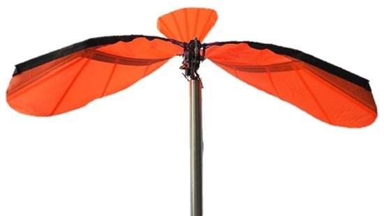
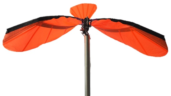
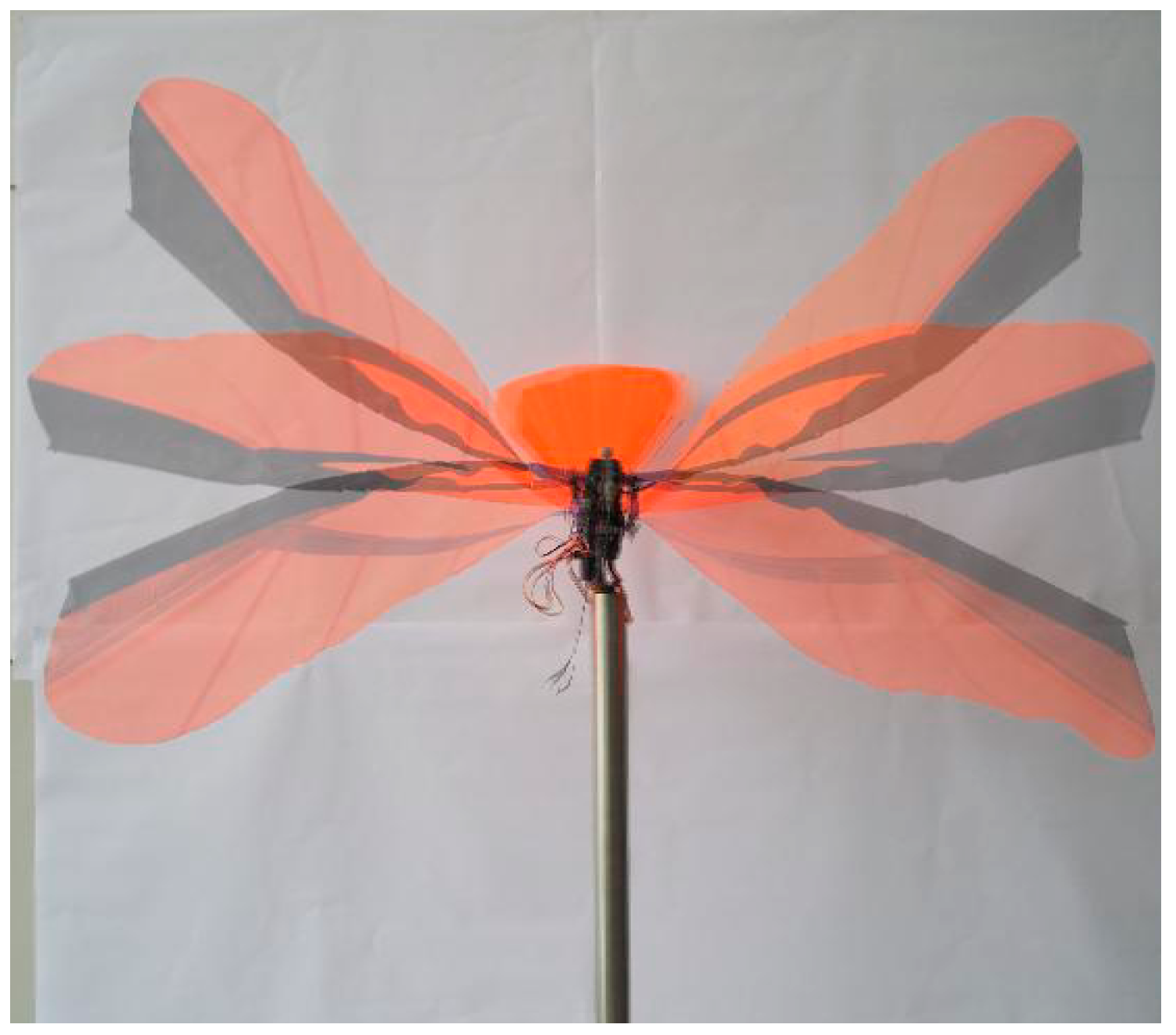
The ornithopter studied in this experiment (see Figure 1) is a commercially available ornithopter kit from Carbonsail with a 1.3 m wingspan at the leading edge, remote-controlled by rib-stop fabric [17].

Table 1. Physical and kinematic data of the ornithopter.

Parameters	Values
Mean chord length of each wing	0.455 m
Aspect ratio of each wing	1.42
Mass of the ornithopter	450 g
Flight speed of the ornithopter	10–25 km/h
Range of wingbeat frequency	3.5–4.5 Hz
Reynolds number based on tip speed	For 5.8 m/s (min): 174, 641
	For 7.5 m/s (max): 225, 829

shows the mean chord length and aspect ratio of each wing, the mass of the ornithopter, the flight speed, the range of the wingbeat frequency and the Reynolds number. The kinematic viscosity of the air was used at 1 atm at 20 °C: 1.5 × 10⁻⁵. The maximum tip speed was linearly scaled by comparing the ratio between the tip speed and flapping frequency and scaling the values for maximum and minimum wing frequency at 4.5 and 3.5 Hz, respectively (actual values can be confirm using OptiTrack). At 3.5 Hz the wing tip speed is estimated to be 5.8 m/s and at 4.5 Hz it is estimated to be 7.5 m/s.

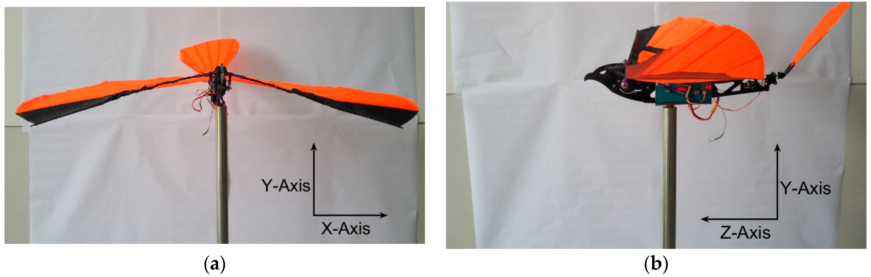
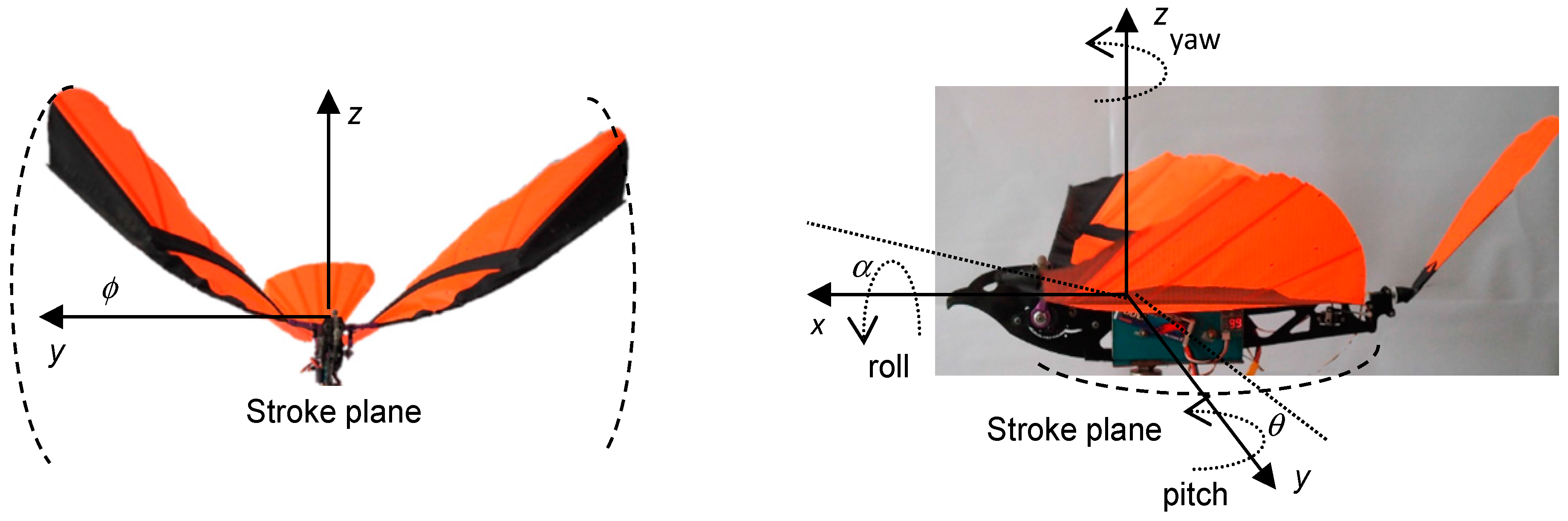
Figure 1 illustrates the axes’ orientation, with respect to the ornithopter, which will be used when describing the kinematic results in the subsequent subsections. A right-handed coordinate system, with its origin at the pivot point was defined as: positive x from the body midline towards the tip of the left wing, positive Y in the vertical upward direction and positive Z from the wing trailing edge to the leading edge direction.

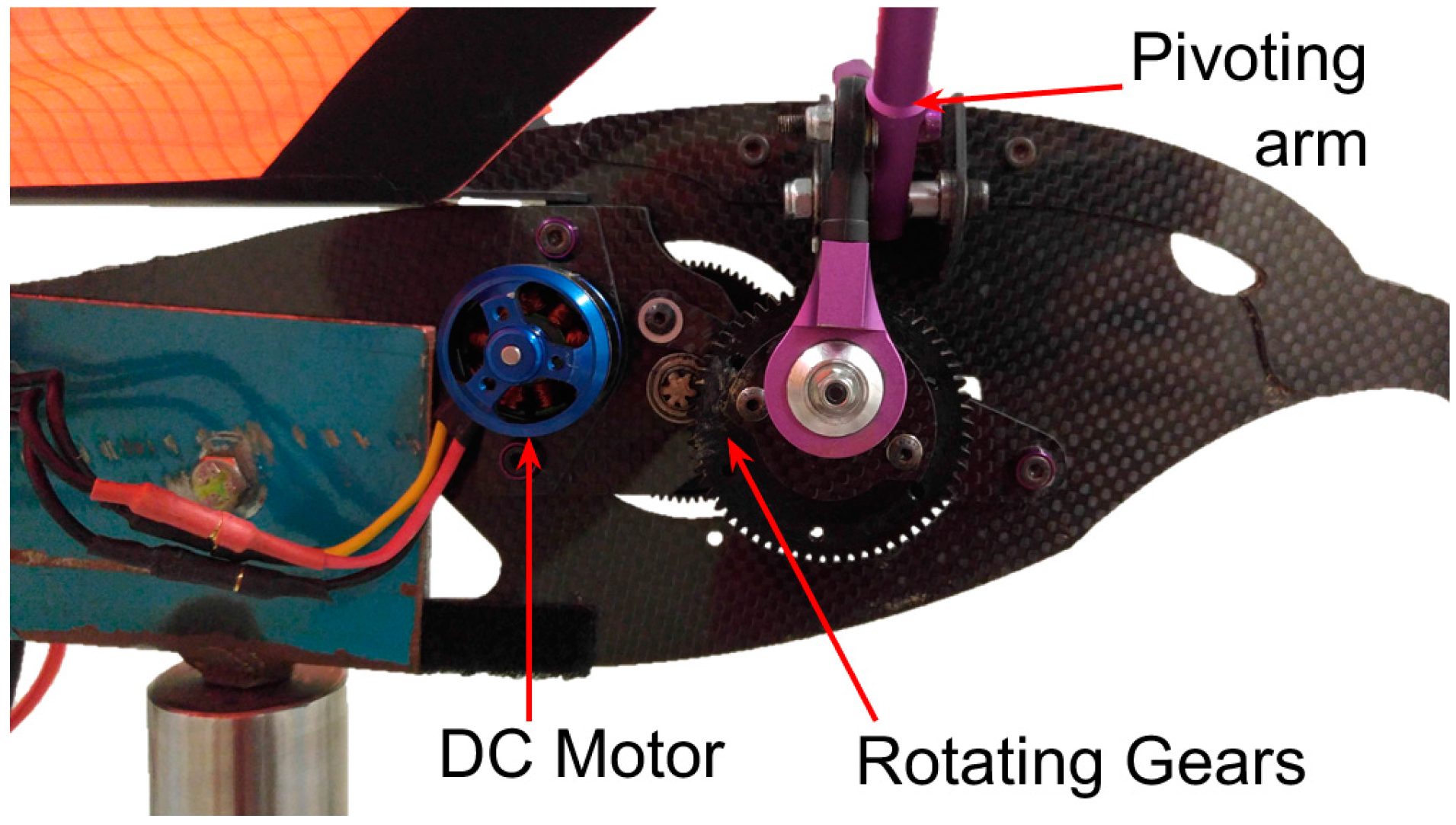
The flapping mechanism used on the ornithopter is of a traverse shaft design (see Figure 2). While the heaviest and most complicated design for flapping mechanisms available, it allows for the most symmetrical flap. The plane of rotation for the rotating gears and the flapping wings are orthogonal; thus, the connector rod has to be able to rotate. A brushless DC motor was used as the actuator to drive the wing flapping mechanism.

3. Experiment Setup and Procedure

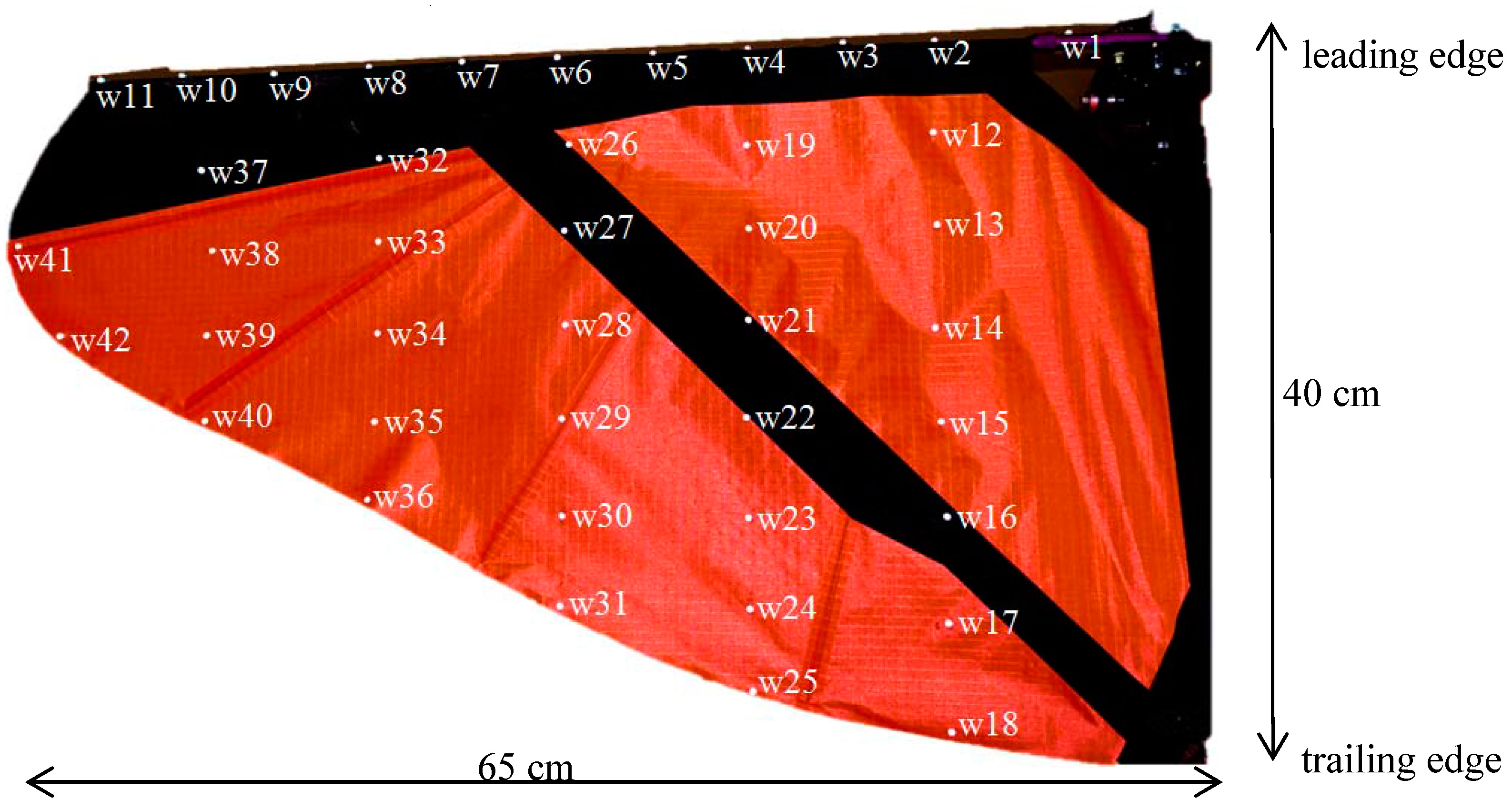
To prepare for the experiments, 42 retro-reflective hemispherical markers of 3 mm diameter were fitted onto the left wing of the ornithopter. The wing was split up into six sections: the leading edge and five “blade elements” along the wing membrane. Markers were placed at a 5 cm interval along both the leading edge spar and each “blade elements”. Each “blade elements” were spaced at 10 cm intervals. Lastly, two markers were placed at the wing tip along the membrane. The markers were labelled from w1 to w42 as shown in Figure 3.

Blade elements are defined as follows: blade element 1 is made up of markers w12 to w18, blade element 2 is made up of markers w19 to w25, blade element 3 is made up of markers w26 to w31, blade element 4 is made up of markers w32 to w36 and blade element 5 is made up of markers w37 to w40. Lastly, the leading edge is defined by markers w1 to w11.

The markers in the case of this experiment are hemispherical and coated with a retroreflective material to reflect light that is generated near the camera lens. To enhance contrast, each camera is equipped with infrared light-emitting diodes and an infrared pass filter that is placed over the camera lens. Motion capture is ideal for capturing the dynamic behaviour of the wing during flight due to its minimal interference with the wing’s motion. Twenty cameras, each capable of recording position data with a precision of +/− 0.1 mm at rates of 360 frames per second, are included in this OptiTrack setup with the capacity of tracking an 8-by-8-meter capture volume. Data captured from the cameras is sent to the optical motion capture software Motive-Tracker [18] where the markers positions are triangulated and the motion is reproduced in a six-degree freedom model.

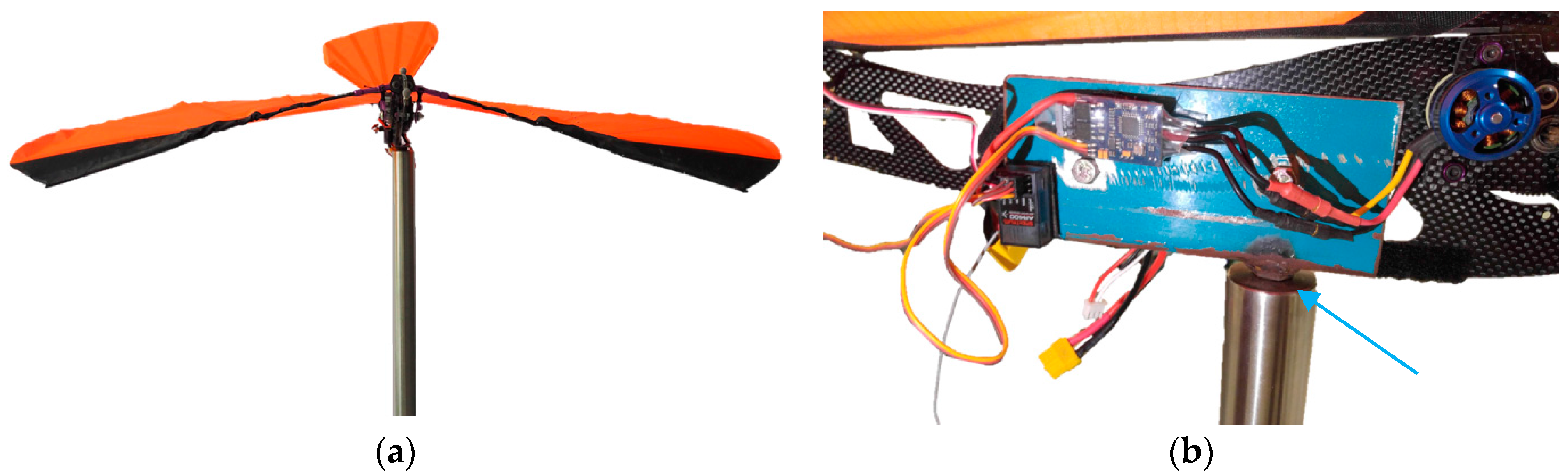
Due to asymmetric plunging of the wing below the ornithopter horizontal axis, a custom test stand (see Figure 4a) and clamp (see Figure 4b) had to be fabricated to accommodate the slim profile of the ornithopter body, while sufficiently alleviating the ornithopter off the ground without impeding wing movement.

Regarding the tracers, according to Harmon et al. [19], the total weight of the markers would have to exceed five grams for the mass of markers to detrimentally affect the wing dynamics. In our experiments, the total weight of the markers fixed onto the ornithopters adds up to 0.42 grams; therefore, we considered any dynamic effects are negligible.

4. Results

4.1. Kinematic Results

This section examines the kinematics of the ornithopter, in particular its wing tip path, leading edge bending and wing membrane shape. For this motion capture take, the wing oscillated at 3.93 Hz when throttle was at 50%. The upward and downward stroke path had been identified by analysing the translational position of the markers from the data exported from Motive.

4.1.1. Wing Tip Path

This experiment demonstrates the trajectories of the wing tip and its deflection from the zero point of the Y-axis (when the wing is horizontal) as captured by the OptiTrack motion tracking system. The left wing leading edge support rod is made from carbon fibre. Due to the possibility of the wing spar flexing, the wing tip path (the tip of the rod furthest from the wing root) was expected to travel in an elliptical or figure-eight motion along the Z–Y axis with minimal flex in the Z-direction, similar to the wingtip strokes of larger birds, while the plot of the wing tip path on the X–Y axis would follow a predictable crescent movement for the entire stroke due to the wing flexing in the Y-direction.

The wing was shown to take a crescent movement as the leading edge flexes during a stroke cycle similar to the front view (X–Y axis) of the wing tip path of birds, while the upstroke is also a crescent shape which is dissimilar as the wing is unable to fold, unlike birds who typically fold their wings in an upstroke to conserve energy (see Figure 5).

The Z–Y view demonstrates an almost vertical stroke plane (see Figure 6) with a mean stroke plane angle of 83.5°. While the motion of the wing tips out of the stroke plane is small, for deflections along the Z-axis, and while the wing tip took a figure-eight path, there was additional flexing between 0.2 and 0.3 m of the Y-axis as the wing decelerated at the end of an upstroke to transit into a downstroke. This additional bending by observation of a frame-by-frame video of the wing flapping at 50% throttle can be attributed to the elastic energy stored in the wing spar as it travels up and down a stroke; this energy is released when the pivoting arm stops at the end of an upstroke and downstroke causing the wing tip to travel a few additional centimetres. It was also noted that some elastic energy could have been transferred from the stand to the wing when the stand flexed as it resisted the forward thrust of the ornithopter, adding to the Z-axis motion.

4.1.2. Leading Edge Bending

The motivation for analysing the kinematic results of the leading edge bending is due in part to the observation of a large difference in the leading edge flex when comparing a single upstroke to a single downstroke (see Figure 7).

The trajectories of markers w1 to w11 which represented the leading edge of the wing were plotted for the purpose of this experiment. Figure 7 shows the X–Y axis (front view) of the ornithopter at a flapping frequency 3.93 Hz.

In Figure 6b, the wingtip path showed up to 7 cm rearward deflection and 2 cm forward deflection along the Z-axis due to passive leading edge bending in the downstroke phase. The downstroke phase theoretically being the “power” phase is the period in which most of the lift and thrust is generated. The start of each wingbeat cycle was designated as the upper reversal point of the wing tip. A single stroke phase can be subdivided into three sub-phases: (1) initial acceleration; (2) mid-swing; and (3) final deceleration. In addition to the body force acting on the leading edge due to its acceleration through the air, there is a combined vectored force of lift and thrust also acting on the leading edge. As a result, the leading edge experiences high inertial loads, causing it to flex. This flex is greatest at mid-swing when the velocity reaches its peak (see Figure 8a). The velocity of the wing tip peaks at 6.54 m/s at mid-swing. The acceleration in the downstroke phase before the velocity peaks can characteristically be seen in the larger gaps between frames when comparing the top half of the graph to the bottom half. A response to high inertial loading, which is especially strong near the wing tip, increases the local feathering angle. A lag then forms between the wing root and wing tip.

4.1.3. Wing Membrane Shape

Unlike conventional aerial vehicles where the wing profile is generally constant throughout flight, the wing profile of an ornithopter in a single wing-beat cycle is in constant change as it reacts to the changes in airflow and forces acting on the wing. The large degree of bending and twisting visible in the wing is a result of the membrane adjusting its camber and pitch to maintain equal tension throughout its surface when the relative inflow speed and inflow angle change throughout the stroke (see Figure 9).

This subsection examines the nominal wing profile by examining blade element 3, which is located at the center of the wing, at various frames for a single downstroke and upstroke cycle mid-flight.

As the wing is primarily driven by the spar at the leading edge, the trailing edge is expected to always lag with respect to the leading edge. Frames 1 to 3 as seen in Figure 10a show the transition from an upstroke of the previous wing-beat cycle to the start of a downstroke of the current wing-beat cycle. Similarly, Frames 11 to 13 in Figure 10b show the transition from the downstroke to an upstroke. These transition phases demonstrate the lead-lag behaviour of the wing between the leading edge and the trailing edge. This lead-lag behaviour contributes to the twisting motion component of the wing.

4.2. Position Angles

During flapping flight, a bird carries out three essential motions with its wings:

• A vertical flapping motion (up and down);
• A horizontal sweeping motion (forward and backward);
• A torsional motion (twisting of the wing).

These three essential motions of the wing can be realized mathematically by modelling and defining the kinematics of the bird. The wing-beat kinematics is described by three positional angles (see Figure 11).

• Flapping about the X-axis in the wing-fixed coordinates is described as the flapping angle, $\varphi$. It represents the angle between the leading edge of the wing and the horizontal plane.
• Rotation of the wing about the Z-axis is described by the elevation angle, θ.
• Feathering (pitching) of the wing about the Y-axis is described by angle of attack, α. As the angle of attack may vary spanwise depending on the torsional angle, the term “local feathering angle” will be used to describe the angle of attack of a chordwise strip along the wing.

$$\varphi \left(t\right)={\displaystyle \sum _{n=0}^3\left[{\varphi }_{cn}\cos \left(2n\pi ft\right)+{\varphi }_{sn}\sin \left(2n\pi ft\right)\right]}$$

(1)

$$\theta \left(t\right)={\displaystyle \sum _{n=0}^3\left[{\theta }_{cn}\cos \left(2n\pi ft\right)+{\theta }_{sn}\sin \left(2n\pi ft\right)\right]}$$

(2)

$$\alpha \left(t\right)={\displaystyle \sum _{n=0}^3\left[{\alpha }_{cn}\cos \left(2n\pi ft\right)+{\alpha }_{sn}\sin \left(2n\pi ft\right)\right]}$$

(3)

Theorems 1–3. 

These equations represent the Fourier series for flapping angle, $\mathsf{\varphi }$, elevation angle, θ and feathering (pitching) angle, α over periodic motion about the X-axis, Y-axis and Z-axis, respectively. The coefficients $\mathsf{\varphi }$_cn, $\mathsf{\varphi }$_sn, θ_cn, θ_sn, α_cn and α_sn are found empirically.

Knowing these coefficients of the Fourier series, it is possible to mathematically recreate the full range of motion of the ornithopter as captured by OptiTrack.

4.2.1. Flapping Angle

Figure 12 shows the flapping angle of the wing and hinge, the first of the three important kinematic parameters of flapping flight. The points calculated and plotted in Figure 12 are for the wing, measured at the wing tip (in blue), and hinge (orange) for one stroke cycle. The period was found to be 0.252 s. Sinusoidal variation of the flapping angle is between +37.58° and −20.16° for the wing and between +31.78° and −7.69° for the hinge. Due to flexing of the leading edge spar, the tip lags behind the hinge by 0.02 s and increases the flapping angle by +6° and −13°. The 0.02 s lag translates to a 28.57° phase lag of the tip to the root. The reason for the larger deviation lower limit is due to the high inertial loads experienced by the spar during a downstroke, which directly translate to larger bending force at the end of the downstroke.

The flapping angle for 5 s of flight was plotted. Figure 13 shows the curve-fitting solution by the MATLAB curve fitting tool. As specified by the Fourier series for periodic motion about the X-axis, the minimum number of the coefficient selected to fit the curve is three terms as shown in

Table 2. Fourier coefficients for flapping angle. The angles are in radians.

Fourier Coefficients
$\mathsf{\varphi }$0 = 0.1192
$\mathsf{\varphi }$c1 = −0.3018	Φs1 = −0.3905
$\mathsf{\varphi }$c2 = −0.01042	Φs2 = −0.02967
$\mathsf{\varphi }$c3 = −0.002753	Φs3 = −0.001312

.

4.2.2. Elevation Angle

Figure 14 shows the elevation angle of the wing, the second of the three important kinematic parameters of flapping flight. Since the wing is incapable of sweeping, theoretically the elevation angle should be zero because the ornithopter was recorded in “hover condition” (the ornithopter was structurally fixed to a stand). As such, the varying angle, however minimal, from +2.65° to −7.98° for this kinematic parameter, is assumed to be due to vibrations transferred from the stand to the wing when the stand flexed as it resisted the forward thrust of the ornithopter.

Similarly, the elevation angle for 5 s of flight was plotted. Figure 15 shows the curve-fitting solution by the MATLAB curve-fitting tool. As specified by Fourier series for periodic motion about the Y-axis, the minimum number of the coefficient selected to fit the curve is three terms as shown in

Table 3. Fourier coefficients for elevation angle. The angles are in radians.

Fourier Coefficients
θ0 = −0.04158
θc1 = 0.02093	θs1 = −0.03674
θc2 = −0.03815	θs2 = −0.01785
θc3 = −0.0006423	θs3 = 0.003587

.

4.2.3. Feathering Angle

Figure 16 shows the feathering angle of the wing, the last of the three important kinematic parameters of flapping flight. The lead-lag nature of the wing both chordwise and spanwise, when coupled together, contributed to the torsional rotation of the wing. The points calculated and plotted in Figure 16 are for the wing, measured at the blade element 1 (in red), the blade element 3 (blue), and the blade element 5 (orange). These represent the wing root, mid-section and wing tip, respectively. Sinusoidal variation of the feathering angle is between +7.75° and −17.64° for the wing root, between +31.73° and −41.9° for the mid-wing, and between +50.6° and −59.8° for the wing tip. The increase in the local feathering angle from the wing root to the wing tip demonstrates the coupled lead-lag nature of the wing and hence an increasing torsional rotation from root to tip. The trailing edge lags the leading edge by 0.04 s as seen in Figure 17, contributing to the lead-lag nature chordwise. The period is 0.252 s and the 0.04 s delay translates to a 57.14° phase lag of the trailing edge to the leading edge.

Lastly, the feathering angle for 5 s of flight was plotted. Figure 18 shows the curve-fitting solution by the MATLAB curve-fitting tool. As specified by the Fourier series for periodic motion about the Z-axis, the minimum number of the coefficient selected to fit the curve is three terms as shown in

Table 4. Fourier coefficients for the feathering angle. The angles are in radians.

Fourier Coefficients
α0 = −0.09502
αc1 = −0.5728	αs1 = −0.479
αc2 = −0.01803	αs2 = −0.0364
αc3 = −0.1374	αc3 = −0.1374

.

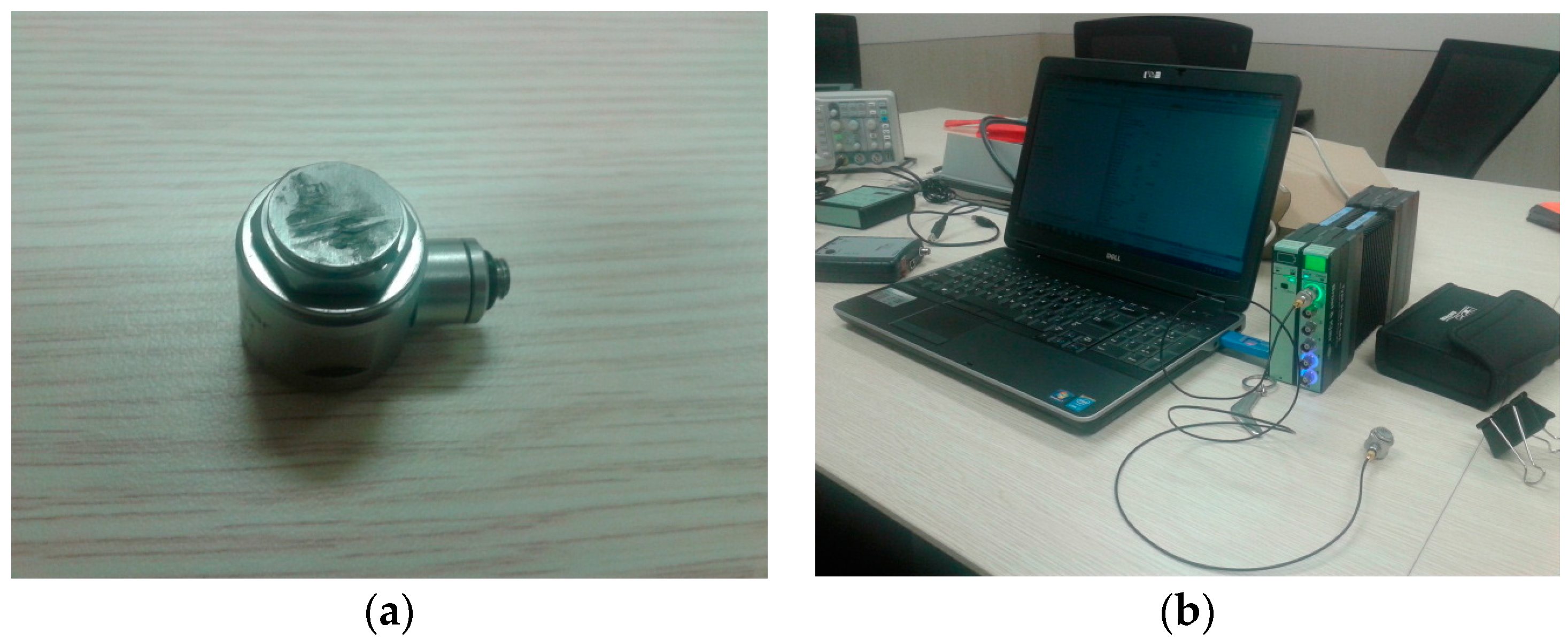
5. Force Measurement

Together with the kinematic data as presented in the previous section, we took measurement of the lift force generated by the flapping motion of this ornithopter. The setup was similar to the one shown in Figure 4a,b. In addition, we installed the force transducer (load cell) at the connecting point between the ornithopter and the support stands, as shown in Figure 4b.

The load cell used was Brüel & Kjær-DeltaTron^® Force Transducers Types 8230, capable of measuring between 0 and 20 N with 0.01 N sensitivity and 0.001 error margin [20], as shown in Figure 19. The measured load data was transmitted to the recording PC [20] via the data acquisition system with the extended Kalman filtering system; hence, the recorded load data was already filtered out of the environment and white noise signals.

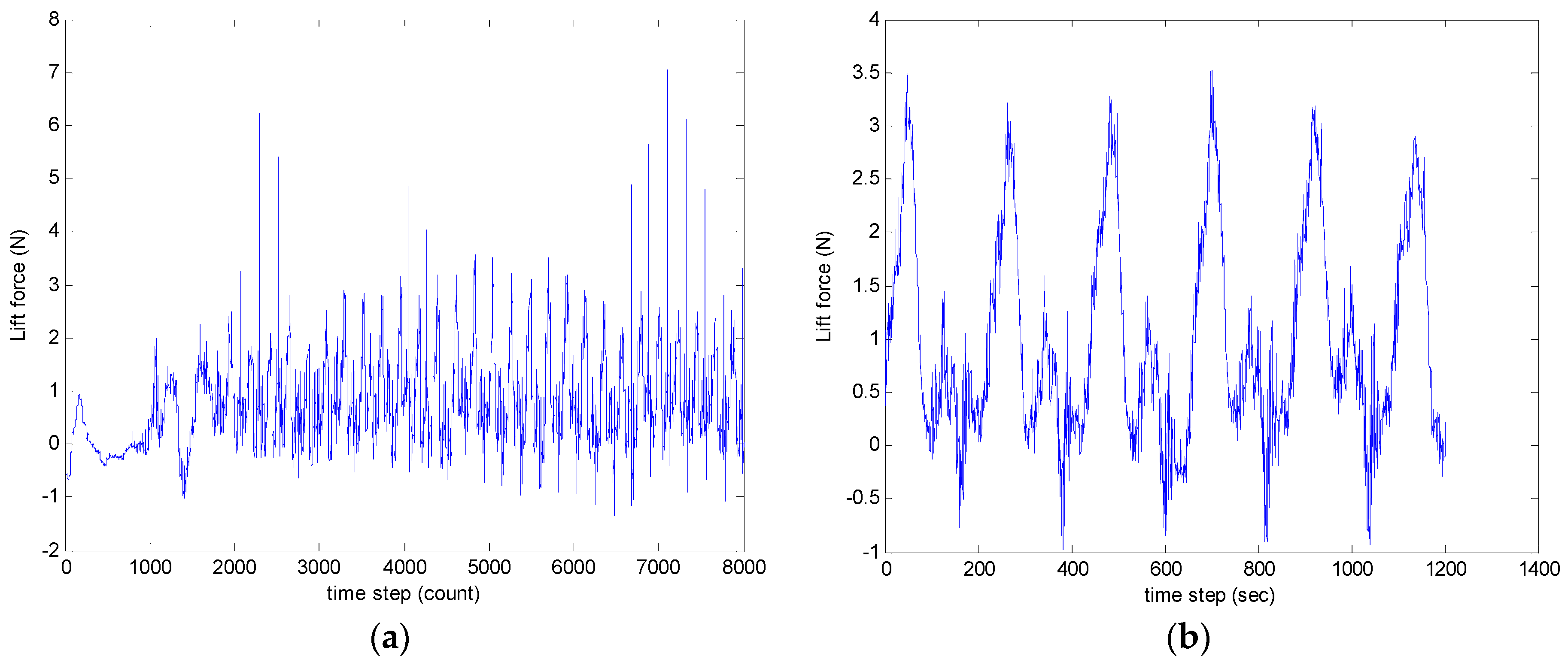
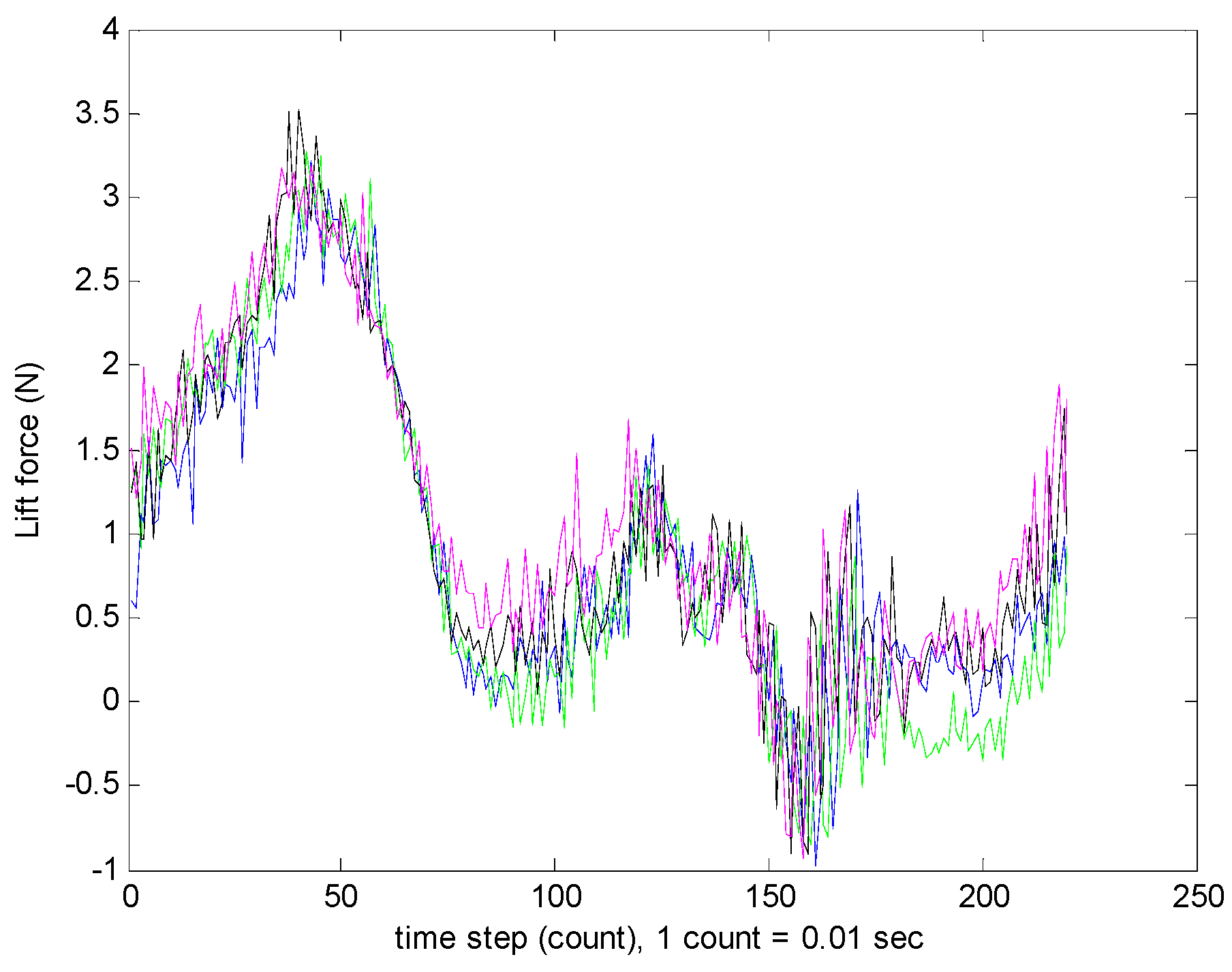
The ornithopter was set to flap at the same condition, i.e., when the wing oscillated at 3.93 Hz. This corresponded to 50% throttle power. The wing was first set to flapping motion for 10 cycles to stabilize the flapping motion, and to let the following flapping motion be steady. Then, we took a recording of the lift force generated for the six subsequent cycles as shown in Figure 20.

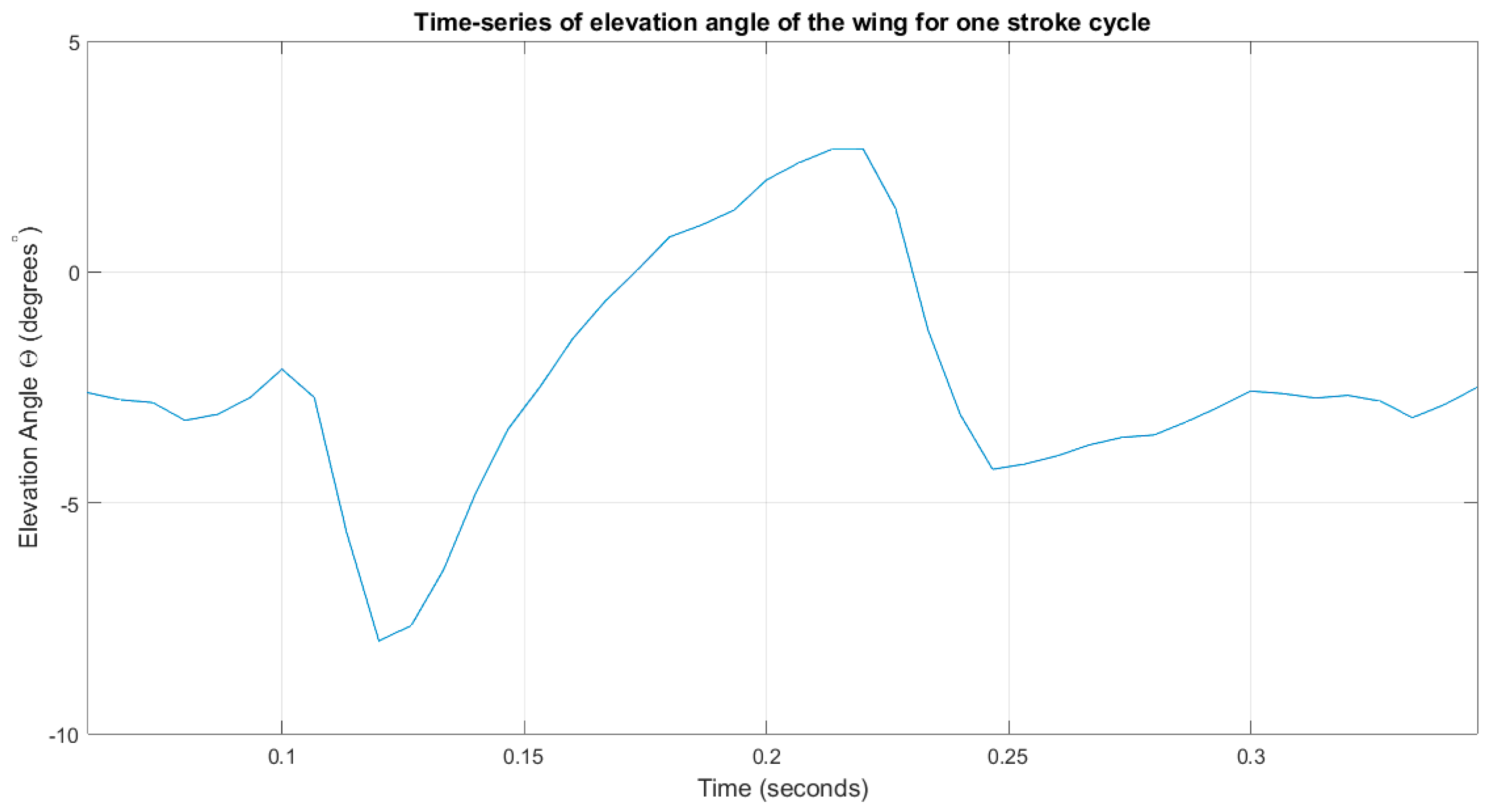
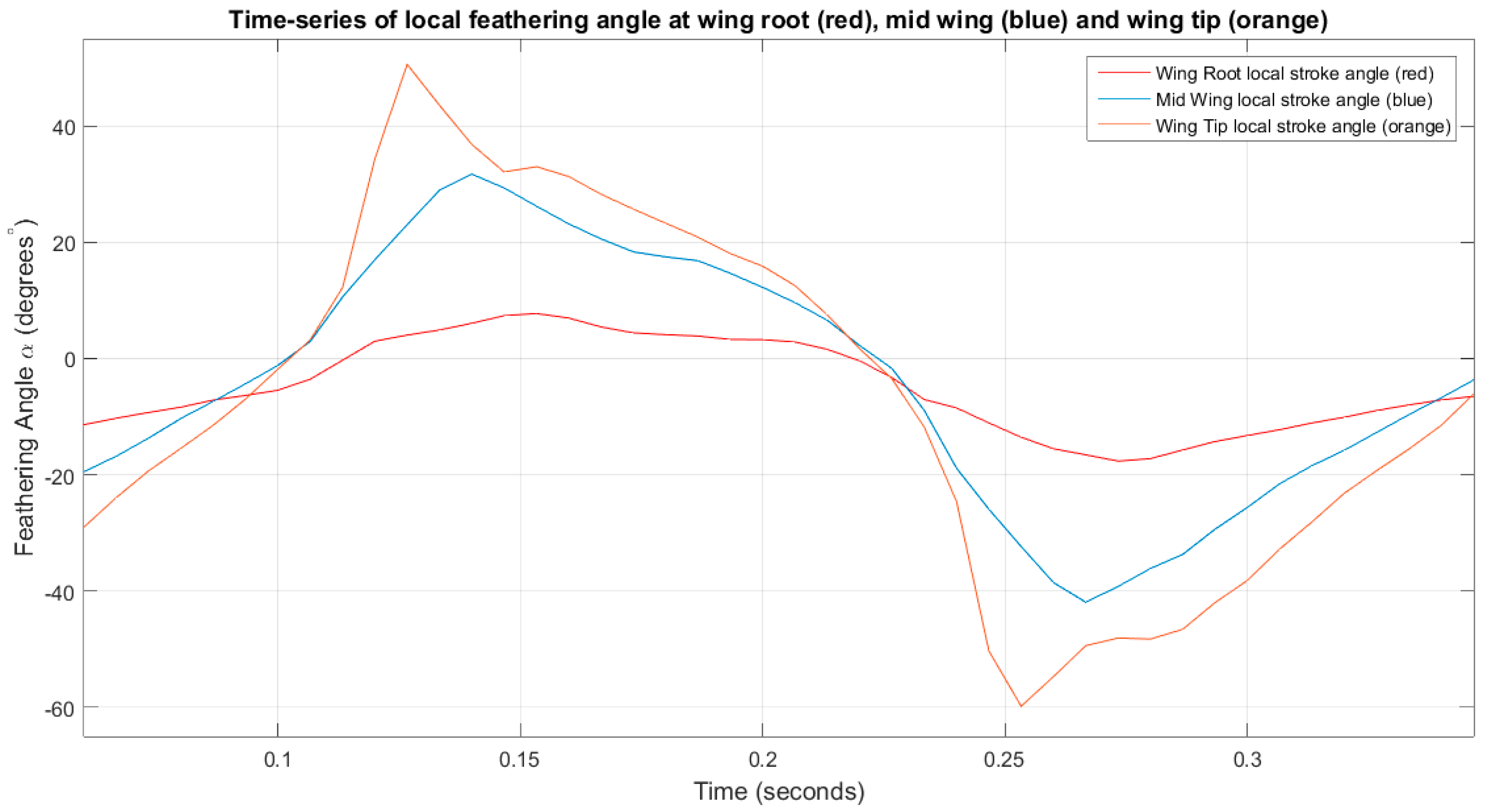
From Figure 20, we noticed that after the 10 initial flapping cycles, the ornithopter could flap more steadily. Figure 21 showed the lift force generated in one cycle, from downstroke (gaining lift) to upstroke (loosing lift). The lift force generation graph resembles the elevation angle plot as presented in Figure 16. We can conclude that it is the elevation angle of the flapping wing that is the main contributor to the amount of the lift, whereas the feathering and flapping angles have a lesser effect.

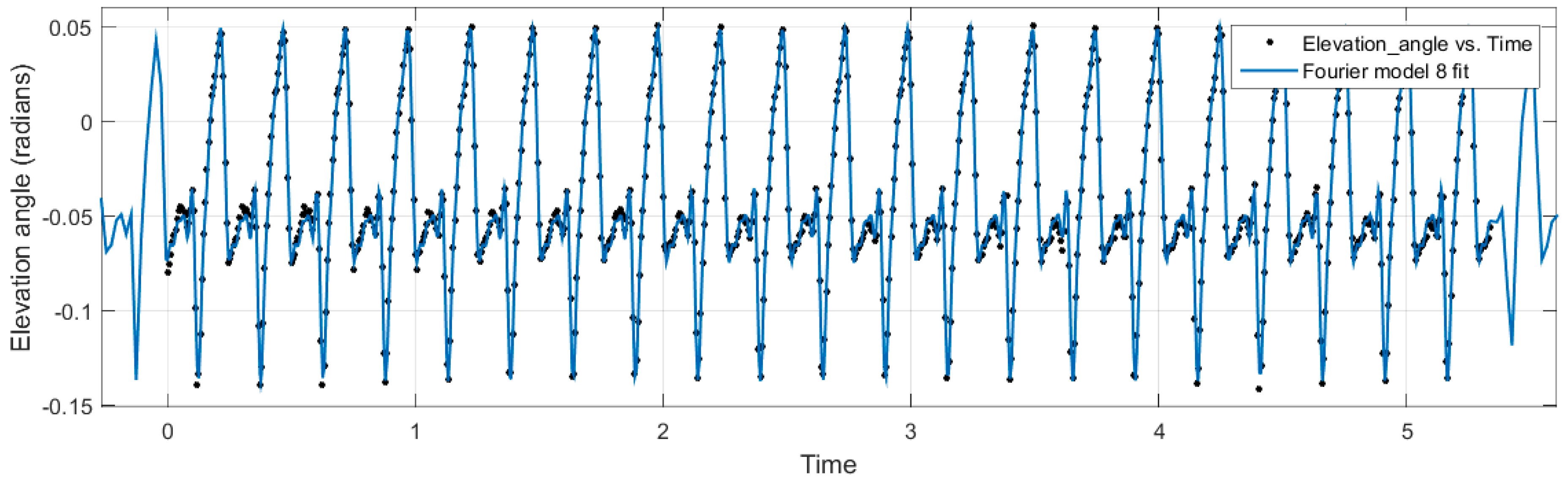
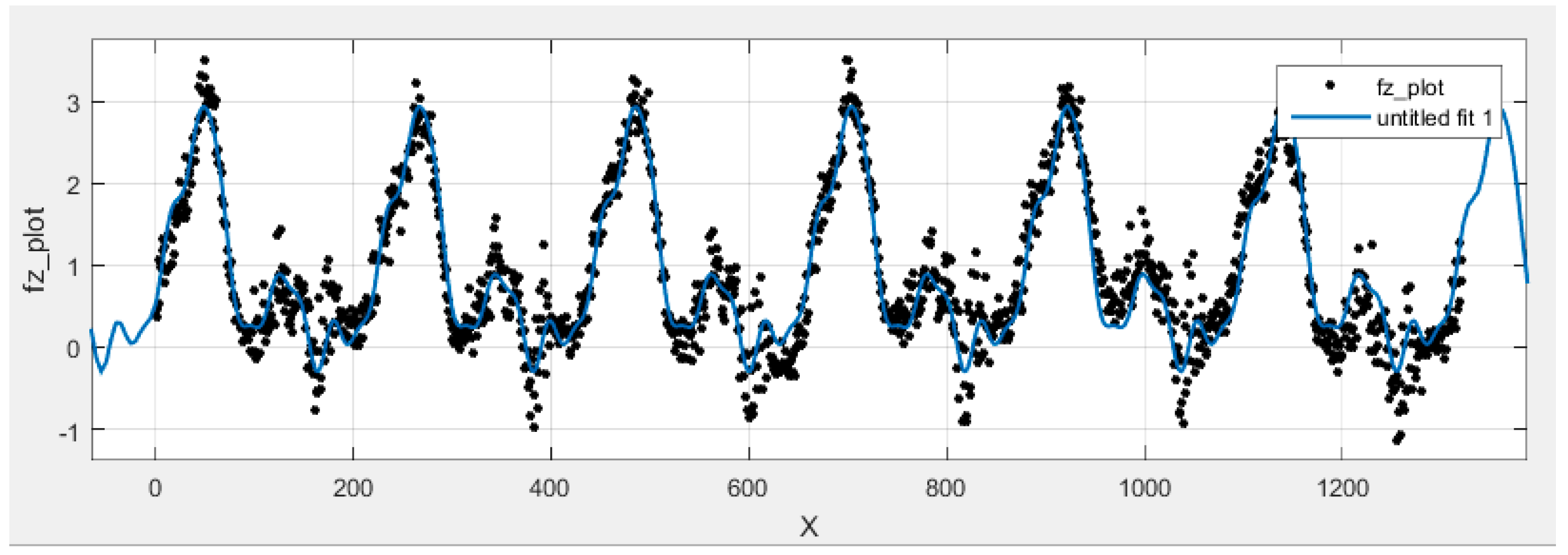
Figure 22 shows the curve-fitting solution by the MATLAB curve-fitting tool. As specified by the Fourier series for lift force, the minimum number of the coefficient selected to fit the curve is eight terms. The coefficients are as listed in

Table 5. Fourier coefficients for the feathering angle.

Fourier Coefficients
α0 = 0.919
α1 = 0.3816	β1 = 0.9566
α2 = −0.2051	β2 = 0.6307
α3 = −0.2635	β3 = −0.2541
α4 = 0.1046	β4 = 0.07073
α5 = 0.1248	β5 = 0.08921
α6 = −0.003921	β6 = 0.002537
α7 = −0.04867	β7 = −0.0009496
α8 = −0.02244	β8 = 0.09985

. The angles are in radians.

6. Discussion

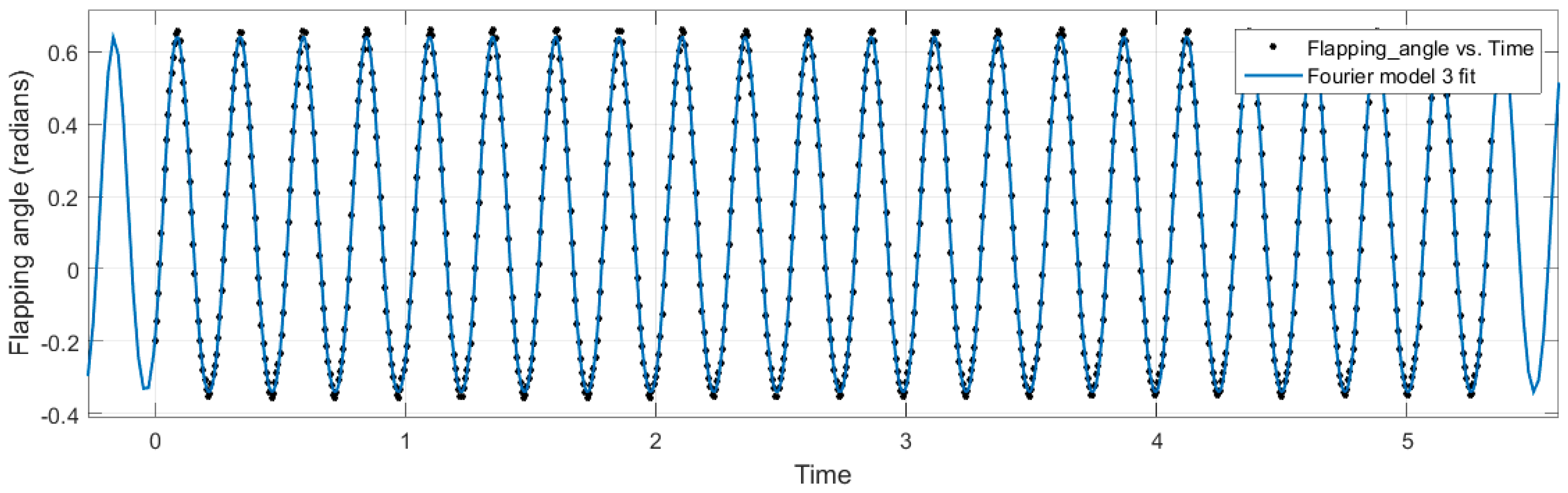
This paper presents the kinematic analysis of an ornithopter wing through motion tracking experiments. The motivation for this research was to isolate the wing geometry and kinematics with time in three-dimensional space and analyse the physical deformation of the wing for a complete stroke cycle. Motivated by the success and quality of the kinematic data, the various position angles were studied and a mathematical equivalent was derived from the empirical data. It was noted during the analysis, however, that for a full and proper curve fit to be made for the data points collected, up to eight Fourier coefficients would have been needed. The values of the fourth to eighth coefficients were so small compared to the first three terms that they were neglected and only the first three terms were considered as the dominating terms.

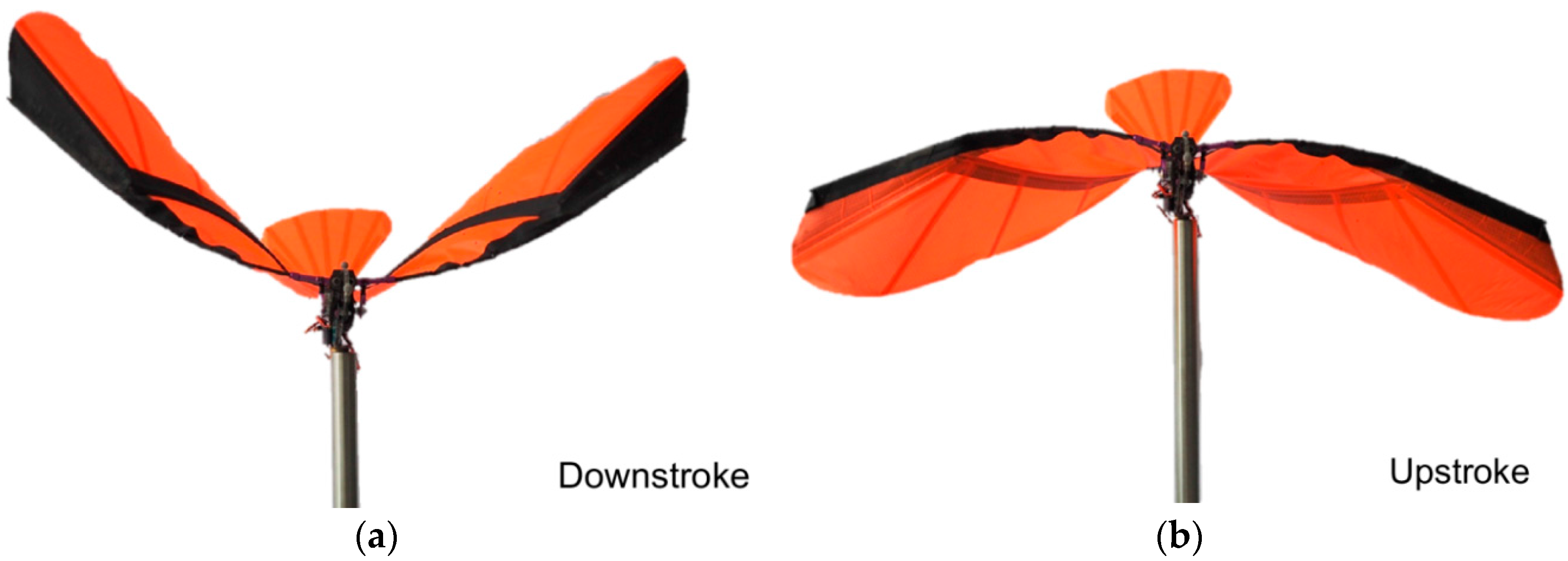
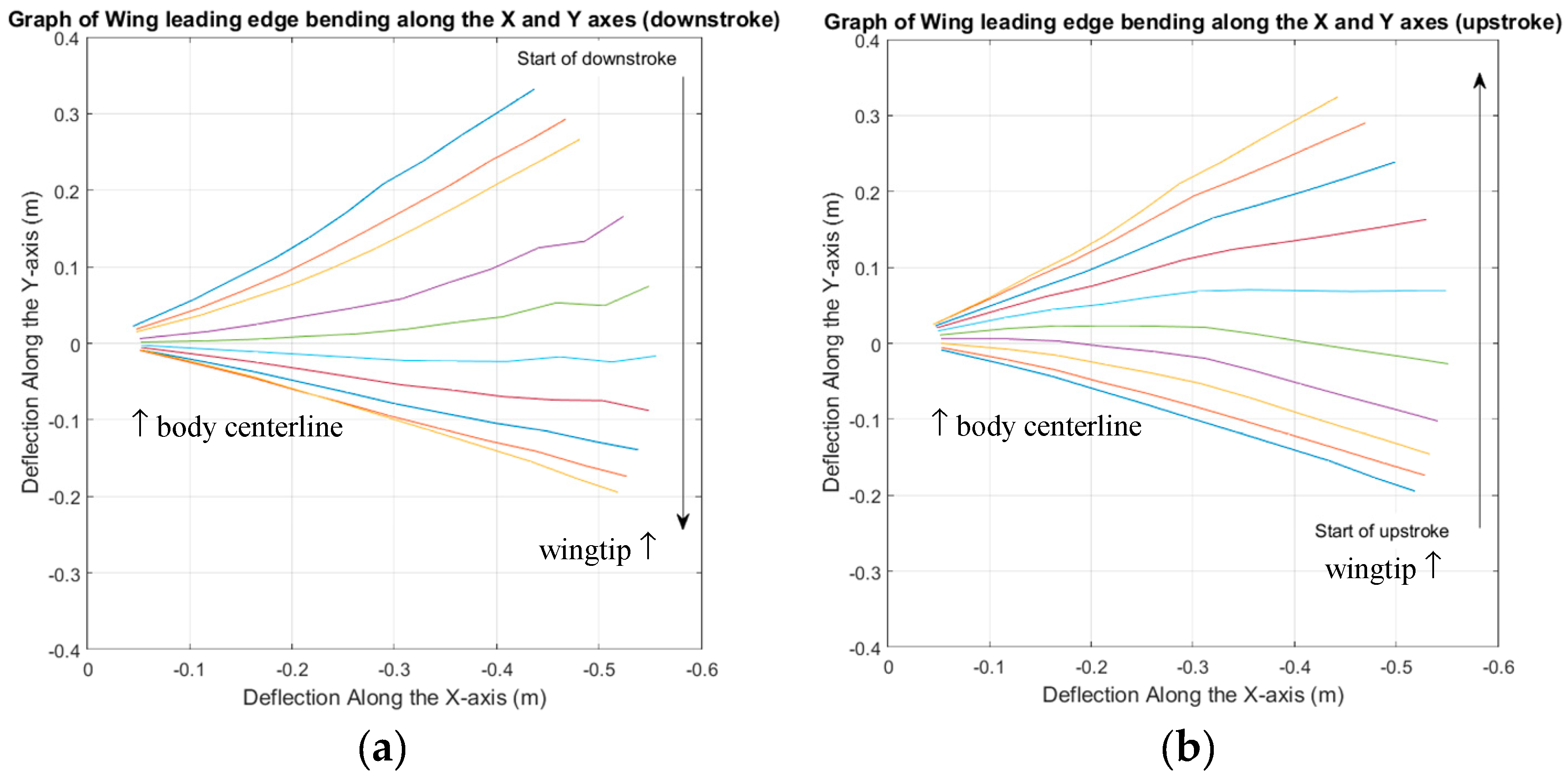
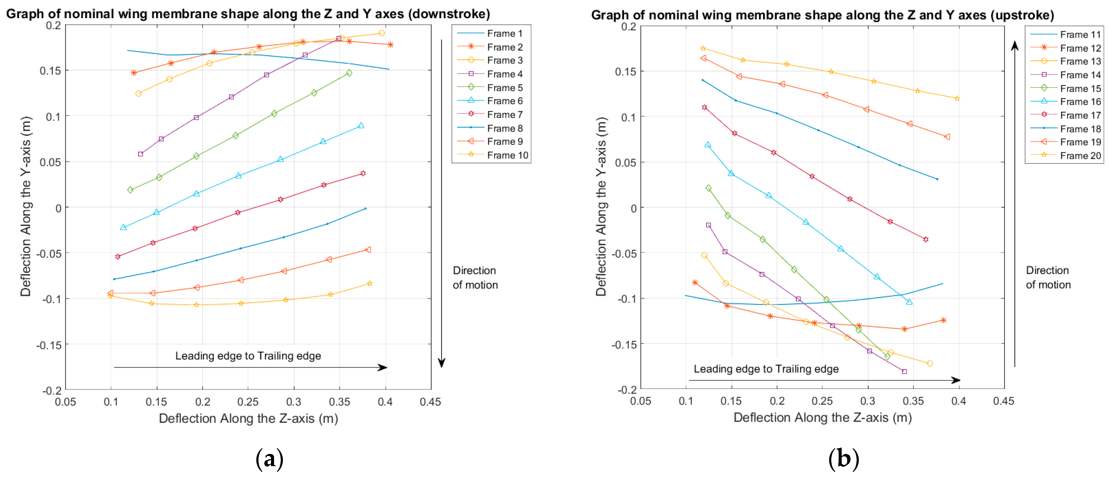
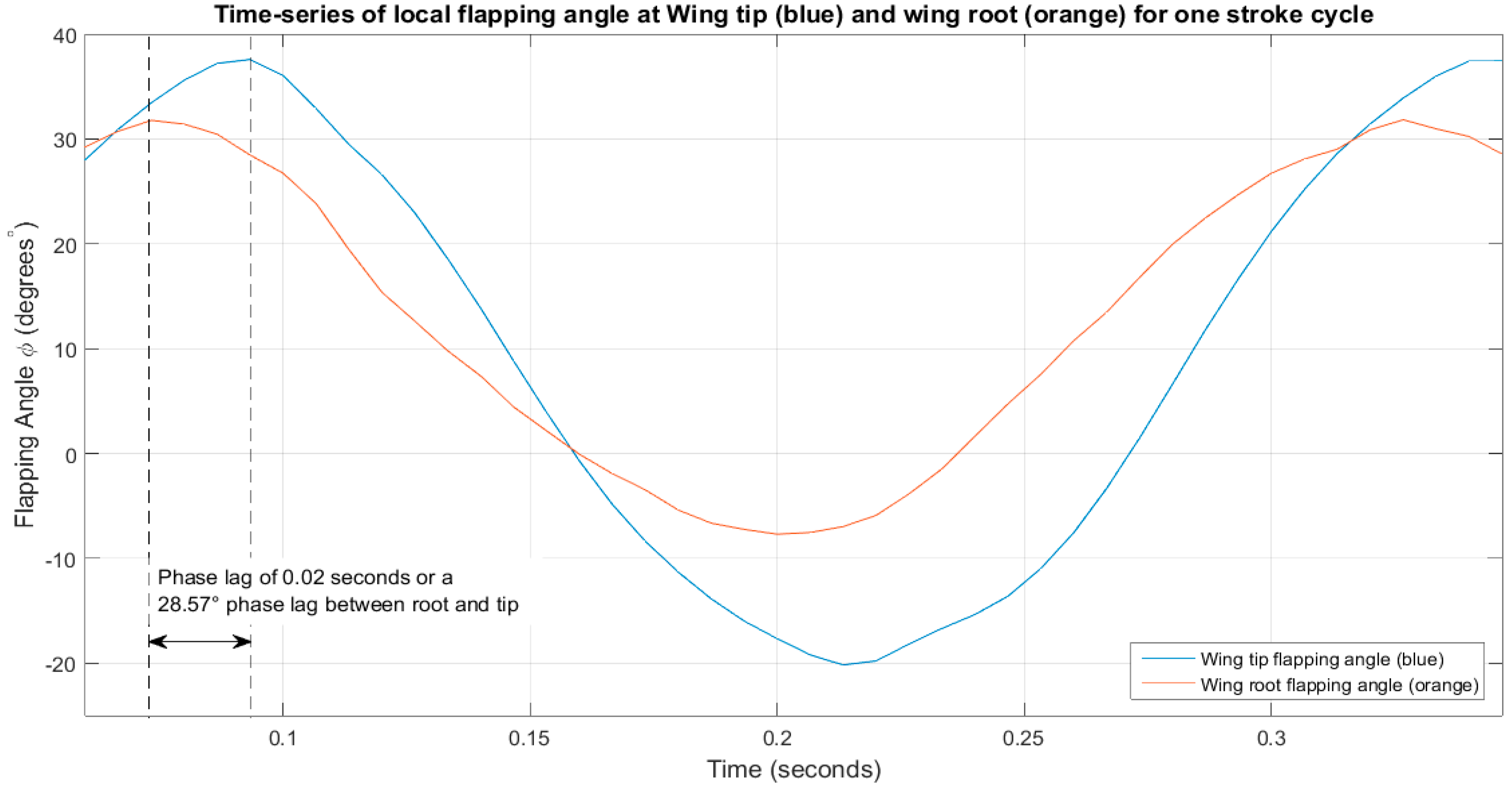
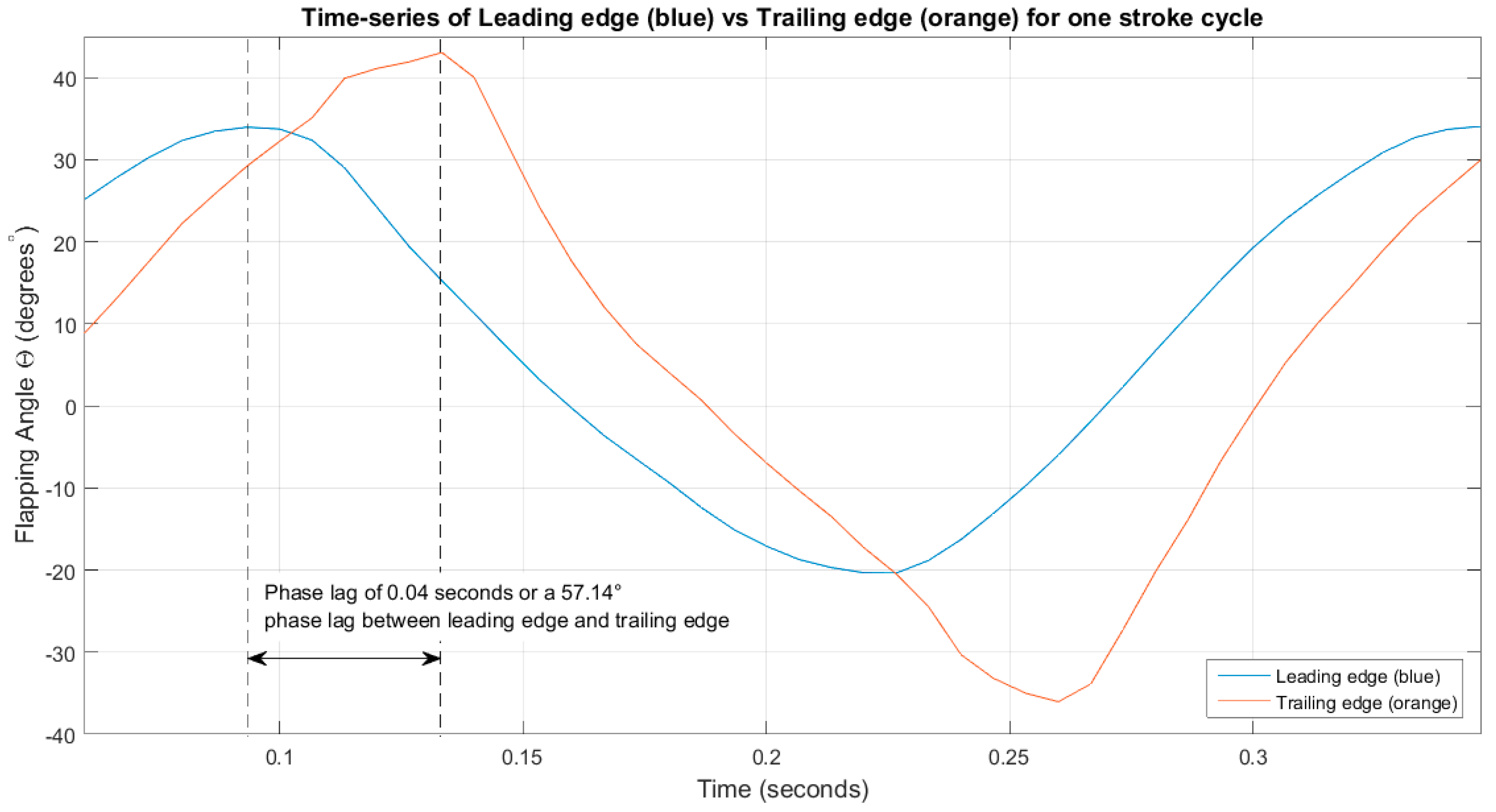
Primary kinematic analysis showed that the ornithopter utilized a vertical stroke plane for flight but experienced significant bending spanwise along the leading edge as well as chordwise pitching along the wing span, similar to what was studied in “Avian flight” and “Animal locomotion” [8,18]. This resulted in the lead-lag nature of the wing with the tip lagging behind the root by 28.57° and the trailing edge lagging behind the leading edge by 57.14°. As such, this resulted in the constant undulating surface of the wing.

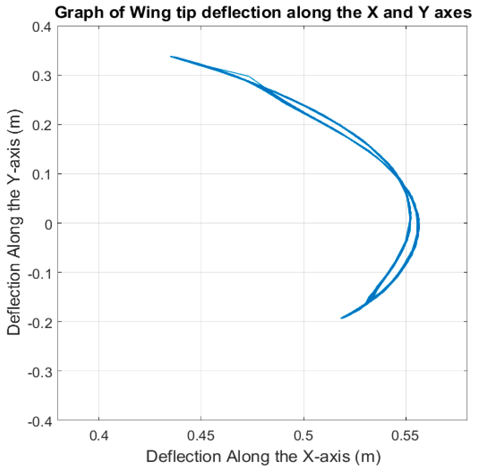
Analysis of the wing tip showed that the wing closely mimics the flight motions of birds with the coupled vertical and horizontal motions replicating the typical figure-eight-shaped kinematics of a bird’s wing. The wing was shown to be highly flexible, capable of achieving high twist angles of +/−50°. The ornithopter also has a higher upper-range flapping angle of +30°; however, the flexing of the wing balances the lower range flapping angle to −20°.

The force reading shows the lift generated follows the elevation of the main flapping wing.

As a next step, we plan to repeat the experiments at various frequencies with the addition of a load test cell to measure the associated lift force and to complete a motion tracking experiment in hover condition at various angles of attack to investigate the effects of gravity on wing bending.

References

1. Alexander, D.E.; Vogel, S. Nature's Flyers: Birds, Insects, and the Biomechanics of Flight; Johns Hopkins University Press: Baltimore, MD, USA, 2004. [Google Scholar]
2. Hall, K.C.; Hall, S.R. Minimum induced power requirements for flapping flight. J. Fluid Mech. 1996, 323, 285–315. [Google Scholar] [CrossRef]
3. De Laurier, J.D. An ornithopter wing design. Can. Aeronaut. Space J. 1994, 40, 10–18. [Google Scholar]
4. Shyy, W.; Lian, Y.; Tang, J.; Viieru, D.; Liu, H. Aerodynamics of Low Reynolds Number Flyers; Cambridge University Press: New York, NY, USA, 2007. [Google Scholar]
5. Wu, T.; Brokaw, C.; Brennen, C. Swimming and Flying in Nature; Plenum Press: New York, NY, USA, 1975; Volumes 1 and 2. [Google Scholar]
6. Harmon, R.L. Aerodynamic Modeling of a Flapping Membrane Wing Using Motion Tracking Experiments. Master Thesis, University of Maryland, College Park, MD, USA, 2008. [Google Scholar]
7. Dial, K.P. Avian forelimb muscles and nonsteady flight: Can birds fly without using the muscles in their wings? The Auk 1992, 109, 874–885. [Google Scholar] [CrossRef]
8. Videler, J.J. Avian Flight; Oxford University Press: Oxford, UK, 2006. [Google Scholar]
9. Pennycuick, C.J. Modelling the Flying Bird; Elsevier: Burlington, MA, USA, 2008. [Google Scholar]
10. Ifju, P.G.; Jenkins, D.A.; Ettinger, S.; Lian, Y.; Shyy, W.; Waszak, M.R. Flexible-Wing-Based Micro Air Vehicles. In Proceedings of 40th AIAA Aerospace Sciences Meeting & Exhibit, Reno, NV, USA, 14–17 January 2002; pp. 1–11.
11. Malik, M.A.; Ahmad, F. Effect of Different Design Parameters on Lift, Thrust, and Drag of an Ornithopter. In Proceedings of the World Congress on Engineering 2010 Vol II WCE 2010, London, UK, 30 June–2 July 2010.
12. Ho, S.; Nassef, H.; Pornsinsirirak, N.; Tai, Y.-C.; Ho, C.-M. Unsteady aerodynamics and flow control for flapping wing flyers. Prog. Aerosp. Sci. 2003, 39, 635–681. [Google Scholar] [CrossRef]
13. Desbiens, A.L.; Chen, Y.; Wood, R.J. A Wing Characterization Method for Flapping-Wing Robotic Insects. In Proceedings of the 2013 IEEE/RSJ International Conference on Intelligent Robots and Systems, Tokyo, Japan, 3–7 November 2013; pp. 1367–1373.
14. Gopalakrishnan, P.; Tafti, D.K. Effect of wing flexibility on lift and thrust production in flapping flight. AIAA J. 2010, 48, 865–877. [Google Scholar] [CrossRef]
15. Fuchiwaki, M.; Tadatsugu, I.; Tanaka, K. Characteristics of Butterfly Wing Motions and Their Application to Micro Flight Robot. In Proceedings of the 48th AIAA Aerospace Sciences Meeting, Orlando, FL, USA, 4–7 January 2010. AIAA paper No.2010-1019.
16. Srigrarom, S.; Chan, W.-L. Ornithopter Type Flapping Wings for Autonomous Micro Air Vehicles. Aerospace 2015, 2, 235–278. [Google Scholar] [CrossRef]
17. Carbonsail Ornithopter. Available online: www.carbonsail.com (accessed on 9 May 2016).
18. OptiTrack Systems. Available online: www.optitrack.com (accessed on 9 May 2016).
19. Harmon, R.L.; Grauer, J.; Hubbard, J.E.; Conroy, J.; Humbert, J.S.; Sitaraman, J.; Roget, B. Experimental Determination of Ornithopter Membrane Wing Shapes Used for Simple Aerodynamic Modeling. In Proceedings of the 26th AIAA Applied Aerodynamics Conference, Honolulu, HI, USA, 18–21 August 2008. AIAA Paper 2008-6237.
20. Bruel & Kjaer Force Transducers Specification. Available online: http://www.bksv.com/Products/transducers/vibration/force-transducers (accessed on 11 July 2016).
Figure 1. (a) Front view of XY axis orientation with respect to the ornithopter; (b) Side view of ZY axis orientation with respect to the ornithopter.
Aerospace 03 00023 g001
Figure 2. Traverse gear mechanism as on the ornithopter platform.
Aerospace 03 00023 g002
Figure 3. Reflective marker layout on the left wing of the ornithopter.
Aerospace 03 00023 g003
Figure 4. (a) Front view of XY axis orientation with respect to the ornithopter; (b) Side view of ZY axis orientation with respect to the ornithopter. The arrow shows the position where the load cell is installed for lift force measurement (Section 5).
Aerospace 03 00023 g004
Figure 5. Graph of the trajectories of the wingtip path for XY axis orientation with respect to the ornithopter.
Aerospace 03 00023 g005
Figure 6. (a) Photography of the side view of the ornithopter, demonstrating the backward to forward sweep of the wing tip in a downstroke; (b) Graph of the trajectories of the wingtip path for ZY axis orientation with respect to the ornithopter.
Aerospace 03 00023 g006
Figure 7. (a) Single downstroke frame of an ornithopter; (b) Single upstroke frame of an ornithopter.
Aerospace 03 00023 g007
Figure 8. (a) Graph of trajectories of leading edge plot for a downstroke; (b) Graph of trajectories of leading edge plot for an upstroke. Different colors refer to different phases of motions.
Aerospace 03 00023 g008
Figure 9. Front view snapshot of the wing at various phases of the stroke cycle. This demonstrates the changing wing profile of the ornithopter.
Aerospace 03 00023 g009
Figure 10. (a) Graph of nominal wing membrane shape along the Z and Y axes of a downstroke; (b) Graph of nominal wing membrane shape along the Z and Y axes of an upstroke.
Aerospace 03 00023 g010
Figure 11. Schematic diagram of wing kinematics.
Aerospace 03 00023 g011
Figure 12. Time-series of local flapping angle at wing tip (blue) and wing root (orange) for one stroke cycle.
Aerospace 03 00023 g012
Figure 13. Fourier curve-fitting solution for flapping angle.
Aerospace 03 00023 g013
Figure 14. Time series of elevation angle of the wing for one stroke cycle.
Aerospace 03 00023 g014
Figure 15. Fourier curve-fitting solution for elevation angle.
Aerospace 03 00023 g015
Figure 16. Time series of local feathering angle at wing root (red), mid-wing (blue) and wing tip (orange).
Aerospace 03 00023 g016
Figure 17. Time series of leading edge (blue) vs. trailing edge (orange) for one stroke cycle.
Aerospace 03 00023 g017
Figure 18. Fourier curve-fitting solution for the feathering angle.
Aerospace 03 00023 g018
Figure 19. Brüel & Kjær-DeltaTron® Force Transducer (a); and its peripherals (b).
Aerospace 03 00023 g019
Figure 20. Lift force generated from start (a); Lift force of the six recorded cycles (b).
Aerospace 03 00023 g020
Figure 21. Lift force generated by the ornithopter in one cycle (from six observed cycles as shown in different colors).
Aerospace 03 00023 g021
Figure 22. Fourier curve-fitting solution for lift force of the six recorded cycles (Figure 20b).
Aerospace 03 00023 g022