Numerical Investigation of Hypersonic Flat-Plate Boundary Layer Transition Subjected to Bi-Frequency Synthetic Jet

Abstract

Transition delaying is of great importance for the drag and heat flux reduction of hypersonic flight vehicles. The first mode, with low frequency, and the second mode, with high frequency, exist simultaneously during the transition through the hypersonic boundary layer. This paper proposes a novel bi-frequency synthetic jet to suppress low- and high-frequency disturbances at the same time. Orthogonal table and variance analyses were used to compare the control effects of jets with different positions (USJ or DSJ), low frequencies (f₁), high frequencies (f₂), and amplitudes (a). Linear stability analysis results show that, in terms of the growth rate varying with the frequency of disturbance, an upstream synthetic jet (USJ) with a specific frequency and amplitude can hinder the growth of both the first and second modes, thereby delaying the transition. On the other hand, a downstream synthetic jet (DSJ), regardless of other parameters, increases flow instability and accelerates the transition, with higher frequencies and amplitudes resulting in greater growth rates for both modes. Low frequencies had a significant effect on the first mode, but a weak effect on the second mode, whereas high frequencies demonstrated a favorable impact on both the first and second modes. In terms of the growth rate varying with the spanwise wave number, the control rule of the same parameter under different spanwise wave numbers was different, resulting in a complex pattern. In order to obtain the optimal delay effect upon transition and improve the stability of the flow, the parameters of the bi-synthetic jet should be selected as follows: position it upstream, with f₁ = 3.56 kHz, f₂ = 89.9 kHz, a = 0.009, so that the maximum growth rate of the first mode is reduced by 9.06% and that of the second mode is reduced by 1.28% compared with the uncontrolled state, where flow field analysis revealed a weakening of the twin lattice structure of pressure pulsation.

1. Introduction

In the design of hypersonic vehicles, the study of boundary layer transition holds significant importance. This is due to the fact that turbulent boundary layers typically exhibit friction drag and heat flux levels that are 3–5 times higher than those of laminar boundary layers [1]. By delaying the transition process, it becomes possible to significantly reduce the friction drag and heat flux of a boundary layer. This, in turn, results in a reduction in the weight of the thermal protection system and an enhancement in both the flight range and payload capacity.

It is generally believed that transition is caused by the evolution of the instability of disturbance over time and space. The process of transition is different depending on the initial disturbance [2,3]. For the different stages of transition, the relevant theories are linear stability theory, nonlinear theory, the receptivity problem [4,5,6], etc. For hypersonic boundary layer transition, in addition to the first mode with low frequency, the second mode with high frequency usually plays a dominant role [7].

Up to now, factors that affect the hypersonic boundary layer transition have been understood to include pressure gradient, surface shape, roughness, wall temperature, total pressure and compressibility [8,9,10]. Transition-delaying control methods are usually divided into passive ones and active ones. The former do not require external energy and do not increase energy consumption, whereas the latter change the flow field through active energy input, which is more efficient.

Common passive transition control methods include vortex generation [11,12], roughness [13,14,15,16,17], wavy wall [17], flexible coating [18], and porous coating [19,20]. The vortex generator has been successfully applied to the air inlet of high supersonic aircraft such as X-43. Paredes [11] studied a vortex generator that delayed transition in a hypersonic boundary dominated by Mack-mode instabilities by inducing streaks. Schneider’s [13] paper outlines three or more modes of transition affected by roughness and indicates that at high hypersonic edge Mach numbers, a very large roughness height is required to influence transition. Fedorov’s [14] study found that the amplitude of the second mode wave is strongest when the two-dimensional roughness is arranged near the synchronization point. The effect of the wavy wall on transition was first studied by Fujii [17], who found that a wavy wall with a wavelength of twice the thickness of the boundary layer arranged in the upstream of the transition region had the effect of delaying transition. Gaponov [18] found that a flexible coating can determine the direction and the degree of the vortex waves of the first mode and the acoustic waves of the second mode. Morozov’s [19] study indicates that under all angles of attack and cone bluntness, the passive porous coating can effectively suppress disturbances in the hypersonic boundary layer on both the windward and leeward sides of the cone.

The active control methods of transition include gas injection [21,22,23], the wall-normal jet [24,25,26], wall heating/cooling [27,28], etc. Germain and Hornung [21] found through wind tunnel experiments that compared with nitrogen and air, carbon dioxide injection has a more significant effect on transition delay. Orlik’s [24] research shows that a low-pressure normal jet is sufficient to effectively inhibit transition, and a non-pulsed jet is more efficient than a pulsed jet. Zhao Rui [27] studied a narrow cooling zone placed upstream of the synchronization point and found its stabilization effect in mode S.

In recent years, active flow control based on synthetic jets has attracted more attention. A synthetic jet with frequency modulation can produce two peaks of low frequency and high frequency, and is referred to as a bi-frequency synthetic jet. It has the advantages of being adjustable and controllable, escaping the shortcomings of passive flow control. Compared to other active control methods, the bi-frequency synthetic jet has a smaller mechanical structure and does not require an additional air source. For hypersonic boundary layer transition, previous methods can only suppress one mode of the disturbance wave, whereas bi-frequency synthetic jets can possess low-frequency and high-frequency control, with the potential to control both the first and second modes simultaneously. This paper describes our attempts to control the first mode with the low-frequency part and the second mode with the high-frequency part of a hypersonic boundary layer based on a proposed bi-frequency synthetic jet. Meanwhile, we employed the orthogonal experiment and analysis of variance to investigate the influences of different frequencies and amplitudes on the transition control effect.

2. Simulation Model

2.1. Freestream Conditions and Numerical Settings

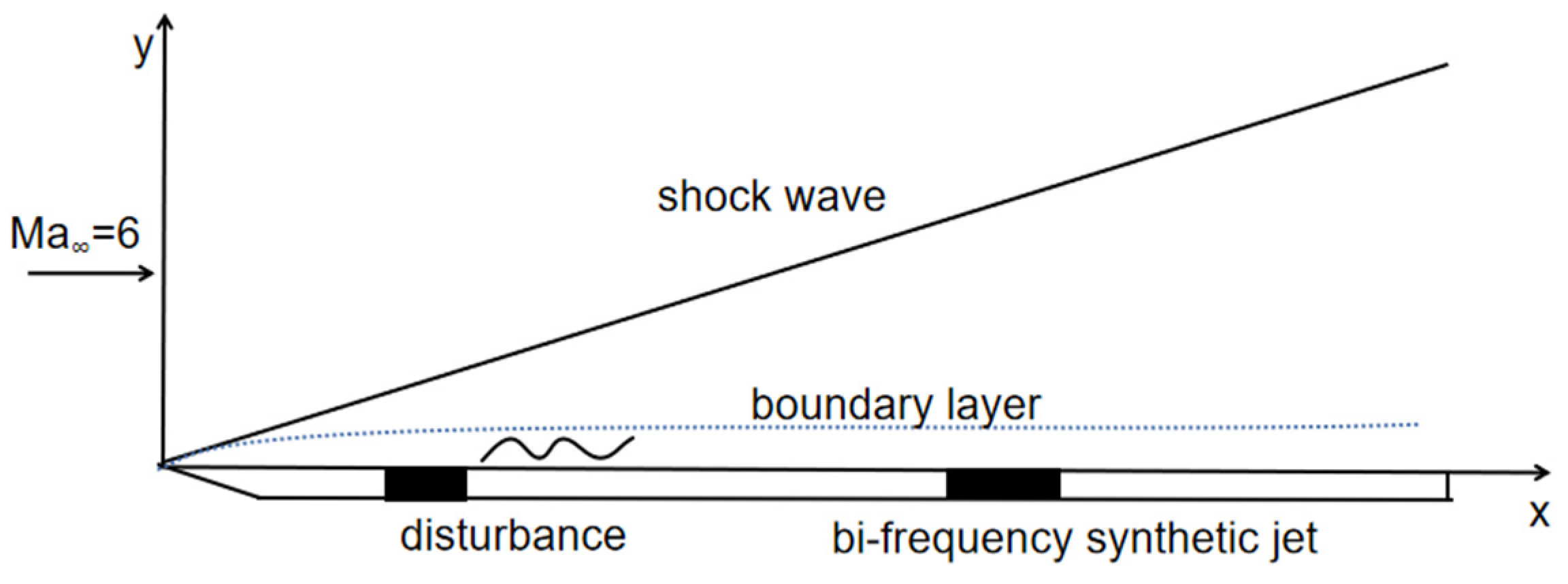
The parameters of the incoming flow described in this paper are consistent with the parameters of the FD-07 wind tunnel at the China Academy of Aerospace Aerodynamics. The Mach number of the incoming flow was 6, the temperature was 54.9 K, and the unit Reynolds number was 1.0 × 10⁷/m. Adiabatic wall conditions were used to simulate the boundary layer of an Ma 6 plate. The model was a sharp plate with a length of 200 mm, as shown in Figure 1. Unsteady blowing and suction disturbance were applied at x = (10 mm, 15 mm). The disturbance form is as follows:

$$q_w=\epsilon \sin (2\pi \frac{x-x_1}{x-x_2})\sin (2\pi ft)$$

The amplitude ε was 0.0001 and the frequency f was 142.54 kHz. The disturbance was added upstream of the flat plate, shown in Figure 1.

For this disturbance, the position of the synchronization point could be calculated by the following formula [29]:

$$x_s^{\ast }=\frac{{(w_{rs}/f)}^2}{{\mathrm{Re}}_{\infty }^2}$$

Therefore, the position of the synchronization point was x = 134.4 mm. Note that we used the boundary layer thickness of x = 100 mm as the reference. From the subsequent simulation results, the boundary layer thickness at this location was found to be δ_ref = 2.07 mm. Therefore, the dimensionless position of the synchronization point was at 64.93 δ_ref.

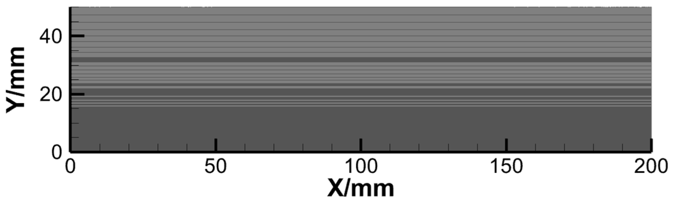
The simulation was conducted using the OpenCFD direct numerical simulation codes developed by Li [30]. The codes use the finite volume method for discretization, the fifth-order WENO [31] scheme to solve the inviscid term, the sixth-order central difference scheme to solve the viscous term, and AUSM [32] to decompose the vector flux. The implicit time step was used to solve the undisturbed laminar boundary layer at first. Then, the disturbance was introduced. The implicit double-time step method was adopted at first, and then the third-order Runge–Kutta method was used to obtain the stable solution with sufficient time accuracy. A grid of 2420 × 401 was used, with grid refinement near the wall, shown in Figure 2. The accuracy of the code and the corresponding mesh and boundary layer velocity profiles have been verified by our team [29].

The bi-frequency synthetic jet can be expressed as follows:

$$v_j=a_1\sin (2\pi f_{1}t)+a_2\sin (2\pi f_{2}t)$$

The low frequency is denoted as f₁, the high frequency as f₂, and the amplitudes as a₁ and a₂. f₁ and f₂ are dimensionless frequencies, obtained by dividing the actual frequency by 890.89 kHz. Similarly, a₁ and a₂ represent the dimensionless amplitudes corresponding to the low and high frequencies, respectively. It is important to note that a₁ and a₂ should be less than 0.01. If they are too large, the nonlinearity will become evident, and the flow will enter a nonlinear process prematurely. In such cases, linear stability theory cannot be applied effectively.

2.2. Orthogonal Experimental Design

Orthogonal experimental design is a rapid method used to study the impact of multiple factors on a given phenomenon [33]. It selects representative combinations of tests from a larger set, allowing for the acquisition of valuable information in a shorter timeframe and with fewer tests.

The orthogonal table L25(5³) was used in this experiment. The total number of trials was 25, 3 factors were tested, and each factor tested 5 levels. Without orthogonal tables, 5³ = 125 trials would be required to test all combinations of the 3 factors with 5 levels, but only 25 times are needed with orthogonal tables. The three factors shown in the table below are the low frequency, f₁, the high frequency, f₂ and the amplitude, a₁ = a₂ = a. The test levels and orthogonal table are shown in

Table 1. Test level.

Level	f1	f2	a
1	0.004/3.56 kHz	0.04/35.63 kHz	0.001
2	0.008/7.12 kHz	0.06/53.45 kHz	0.003
3	0.012/10.69 kHz	0.08/71.27 kHz	0.005
4	0.016/14.25 kHz	0.10/89.09 kHz	0.007
5	0.020/17.82 kHz	0.12/106.91kHz	0.009

and

Table 2. Orthogonal table.

Case	f1	f2	a
1	0.004/3.56 kHz	0.04/35.63 kHz	0.001
2	0.004/3.56 kHz	0.06/53.45 kHz	0.007
3	0.004/3.56 kHz	0.08/71.27 kHz	0.003
4	0.004/3.56 kHz	0.10/89.09 kHz	0.009
5	0.004/3.56 kHz	0.12/106.91 kHz	0.005
6	0.008/7.12 kHz	0.04/35.63 kHz	0.007
7	0.008/7.13 kHz	0.06/53.45 kHz	0.003
8	0.008/7.14 kHz	0.08/71.27 kHz	0.009
9	0.008/7.14 kHz	0.10/89.09 kHz	0.005
10	0.008/7.14 kHz	0.12/106.91 kHz	0.001
11	0.012/10.69 kHz	0.04/35.63 kHz	0.003
12	0.012/10.69 kHz	0.06/53.45 kHz	0.009
13	0.012/10.69 kHz	0.08/71.27 kHz	0.005
14	0.012/10.69 kHz	0.10/89.09 kHz	0.001
15	0.012/10.69 kHz	0.12/106.91 kHz	0.007
16	0.016/14.25 kHz	0.04/35.63 kHz	0.009
17	0.016/14.25 kHz	0.06/53.45 kHz	0.005
18	0.016/14.25 kHz	0.08/71.27 kHz	0.001
19	0.016/14.25 kHz	0.10/89.09 kHz	0.007
20	0.016/14.25 kHz	0.12/106.91 kHz	0.003
21	0.020/17.82 kHz	0.04/35.63 kHz	0.005
22	0.020/17.82 kHz	0.06/53.45 kHz	0.001
23	0.020/17.82 kHz	0.08/71.27 kHz	0.007
24	0.020/17.82 kHz	0.10/89.09 kHz	0.003
25	0.020/17.82 kHz	0.12/106.91 kHz	0.009

.

According to the different positions of the synthetic jet (upstream: 110–120 mm, denoted by USJ; downstream: 150–160 mm, denoted by DSJ, with synchronization point at x = 134.4 mm), two orthogonal tests were carried out, respectively, and the parameters of the orthogonal tables of the two tests were the same; only the position was different. In addition, it was also necessary to calculate the case under the uncontrolled condition.

Multi-factor variance analysis was employed to examine whether a dependent variable was influenced by multiple factors. Additionally, one-way analysis of variance (ANOVA) was utilized to determine the impacts of different levels of an independent factor on the dependent variable. Traditional methods of studying the effect of a factor by fixing the levels of other factors and only changing the level of the factor under investigation are susceptible to the fixed levels of other factors. However, in one-way analysis of variance, the test cases in the orthogonal table are uniform and organized, allowing for more test cases at the same level as the factors being studied, including all levels of other factors. This enables the average value to eliminate the influence of other factors.

For instance, if we need to study the influence of f₁ = 3.56 kHz, we can consider the first to fifth test cases in the orthogonal table where f₁ = 3.56 kHz. The f₂ of these cases range from 35.63 kHz to 106.91 kHz and their a range from 0.001 to 0.009. By uniformly covering all levels of f₂ and a, we can calculate the average value of the test results from cases 1 to 5 to obtain the influence of f₁ = 3.56 kHz. This approach helps to avoid the influence of specific values of f₂ and a.

2.3. Linear Stability Theory

Linear stability theory is a systematic theory for the study of flow transition [34]. It relies on the assumption of parallel flow and small disturbances to analyze the temporal and spatial evolution of small perturbation waves. These disturbances are typically represented in the form of a wave function:

$$q^{\prime }(x,y,z,t)=\widehat{q}(x,y,z,t)\exp [i(\alpha x+\beta z-\omega t)]$$

where α and β represent the wave numbers in the flow direction and spanwise direction, respectively, and ω denotes the frequency. In the spatial mode, the imaginary part of the flow direction wave number α_i indicates the growth or attenuation of the disturbance, with α_i < 0 indicating growth. For the sake of clarity, this paper adopts the notation −α_i to denote the growth rate, where −α_i > 0 signifies perturbation growth, leading to a decrease in flow stability. The objective of this study was to identify a synthetic jet with specific parameters that can effectively control the growth rate −α_i, ensuring it is lower than that observed in the uncontrolled state, so as to suppress the growth of unstable disturbances and enhance flow stability.

To calculate the disturbance, the flow field needs to be decomposed into the sum of average flow and disturbance:

$$q(x,y,z,t)=\overline{q}(x,y,z,t)+q^{\prime }(x,y,z,t)$$

The parallel flow hypothesis was introduced, which holds that the change of the variable in the flow direction is small and negligible, that is:

$$\overline{\rho }=\overline{u}=\overline{T}=f(y)$$

$$\overline{v}=\overline{u}=0$$

By incorporating disturbance and the parallel flow hypothesis into the governing equation and simplifying it, we obtained the linear perturbation equation, or O-S equation [35]. The numerical solution of this equation is referred to as the T-S wave, and the process of solving the O-S equation and analyzing the solution is known as linear stability analysis.

For this paper, we conducted linear stability analysis on cases with different parameters, as well as the uncontrolled case; then, the unstable mode growth rate −α_i of each case with variations in the frequency ω_r and the spanwise wave number β_r were obtained. Finally, the results were tested by multi-factor and one-way ANOVA to find the control rules of low frequency, high frequency, amplitude and position.

3. Variation in Growth Rate with Frequency

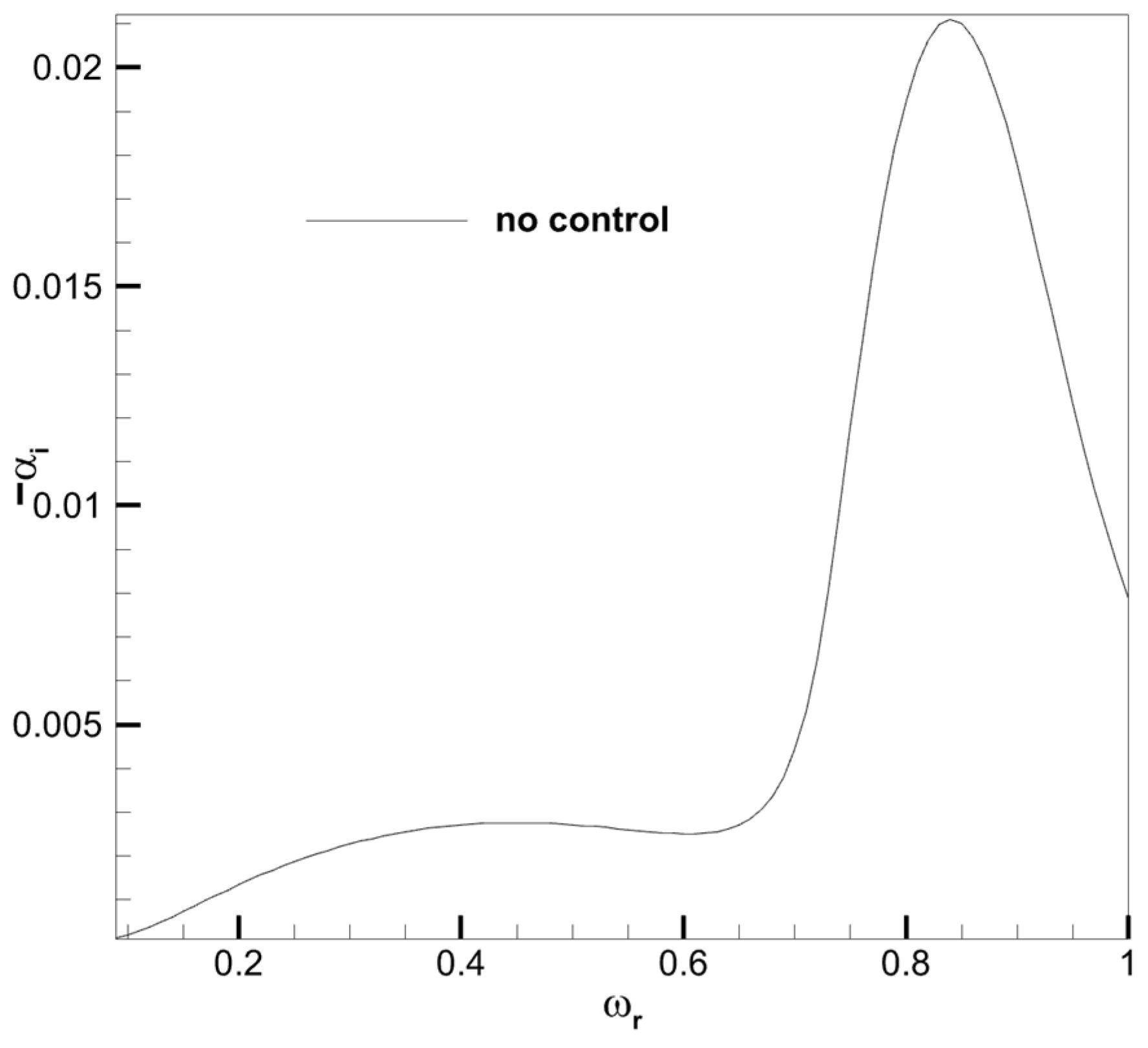
Figure 3 shows the growth rate −α_i varying with frequency ω_r in the uncontrolled case. It is worth noting that the actual frequency is expressed as ω_r × 141.79 kHz. The figure displays two prominent peaks: the first mode (around 63.8 kHz) with a maximum growth rate of 0.00276, and the second mode (around 119.10 kHz) with a higher maximum growth rate of 0.02108. Notably, the second mode emerged as the dominant unstable mode within the hypersonic boundary layer.

3.1. Results of Synthetic Jet Arranged Upstream of Synchronization Point

The maximum growth rates of the first mode and the second mode of each test case with a bi-synthetic jet arranged upstream (USJ) are shown in the second and third columns of

Table 3. Test results of each case of USJ.

Case	Maximum Growth Rate		Percentage of Control
	First Mode	Second Mode	First Mode	Second Mode
1	0.00286	0.02123	3.62%	0.71%
2	0.00286	0.02113	3.62%	0.24%
3	0.00276	0.02118	0.00%	0.47%
4	0.00251	0.02081	−9.06%	−1.28%
5	0.00264	0.02125	−4.35%	0.81%
6	0.00286	0.02126	3.62%	0.85%
7	0.00281	0.02124	1.81%	0.76%
8	0.00257	0.02108	−6.88%	0.00%
9	0.00262	0.02096	−5.07%	−0.57%
10	0.00278	0.02119	0.72%	0.52%
11	0.00283	0.02122	2.54%	0.66%
12	0.00286	0.02128	3.62%	0.95%
13	0.00269	0.02116	−2.54%	0.38%
14	0.00278	0.02115	0.72%	0.33%
15	0.00256	0.02130	−7.25%	1.04%
16	0.00294	0.02136	6.52%	1.33%
17	0.00284	0.02126	2.90%	0.85%
18	0.0028	0.02119	1.45%	0.52%
19	0.00261	0.02096	−5.43%	−0.57%
20	0.00274	0.02129	−0.72%	1.00%
21	0.00288	0.02126	4.35%	0.85%
22	0.00282	0.02121	2.17%	0.62%
23	0.00268	0.02125	−2.90%	0.81%
24	0.00271	0.02107	−1.81%	−0.05%
25	0.00244	0.02119	−11.59%	0.52%

. The fourth and fifth columns are the percentages of promotion or suppression of the first and second modes relative to the uncontrolled case. Positive values represent promotion and negative values represent suppression. It is evident that certain cases promote both modes, some suppress both, and some promote the second mode while suppressing the first mode.

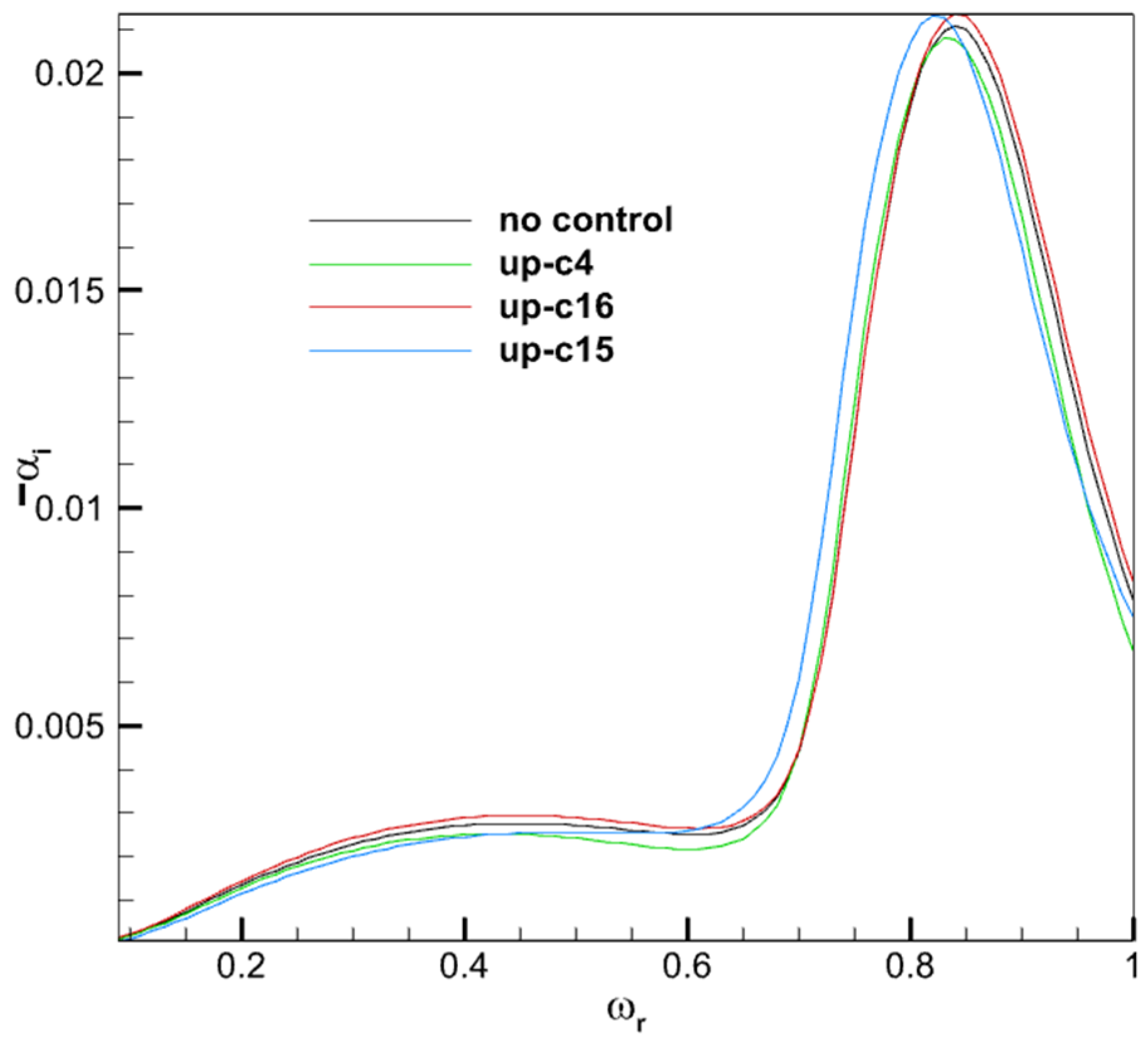
Among all the cases of the USJ, case 16 exhibited the most pronounced promotion effects on both the first and second modes, with increases of 6.52% and 1.33%, respectively. Conversely, case 4 demonstrated the strongest suppressing effects on both the first and second modes, with reductions of −9.06% and −1.28%, respectively. Notably, the 15th case suppressed the first mode by −7.25%, while simultaneously promoting the second mode by 1.04%, as shown in Figure 4.

Table 4. Multivariate ANOVA results of the first and second mode of the USJ.

Source of Variance	p
	First Mode	Second Mode
f1	0.593	0.316
f2	0.003	0.005
a	0.132	0.845

presents the results of the multi-factor variance analysis, examining the controlling effect of the USJ on the first and second modes. In both modes, the p-value for f₂ is less than 0.05, indicating a significant difference among the effects of the levels of f₂ [33]. However, the differences observed among f₁ and a are relatively small.

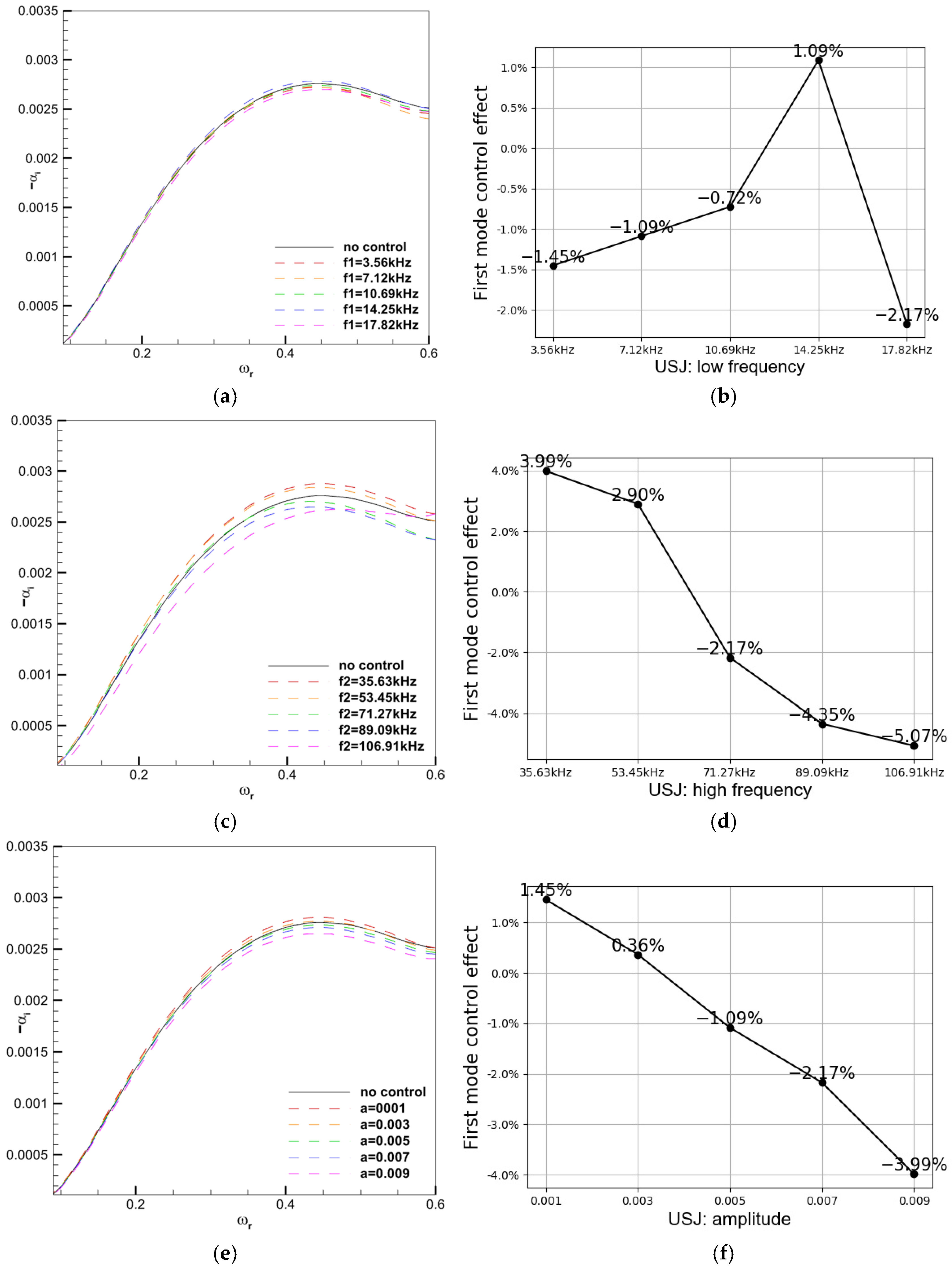
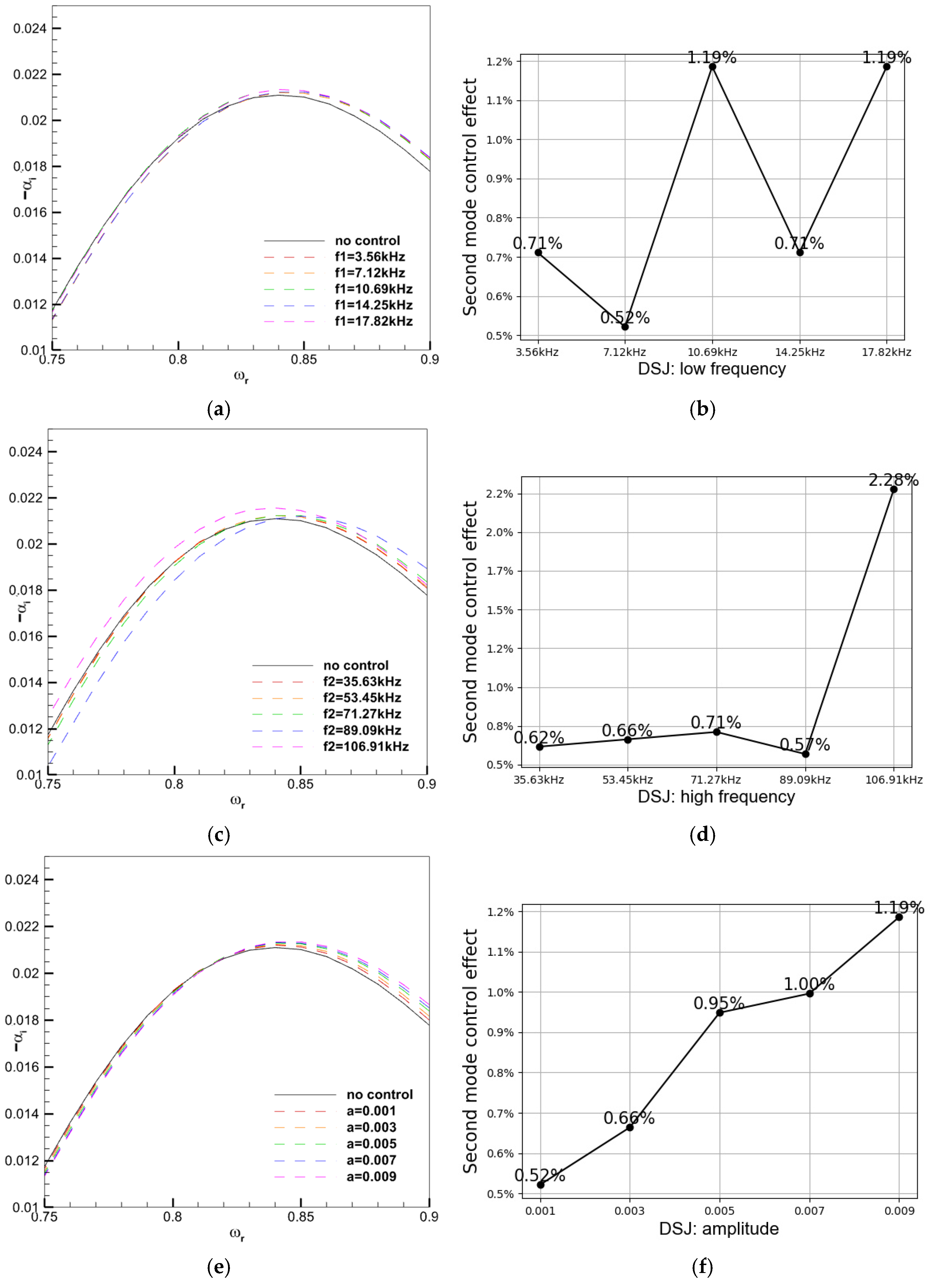
One-way ANOVA was conducted to analyze the first-mode growth rates as the frequency changed, controlled by the low frequency, high frequency and amplitude of the USJ, as shown in Figure 5. For this section, the spanwise wave number β_r was fixed at β_r = 0. For the first mode, when the low frequency, f_1, was too low or too high, the growth rate was lower compared to the uncontrolled state. Additionally, as f₂ increased and a became larger, the first-mode growth rate decreased. These observations reveal enhanced flow stability and a delay in the transition process.

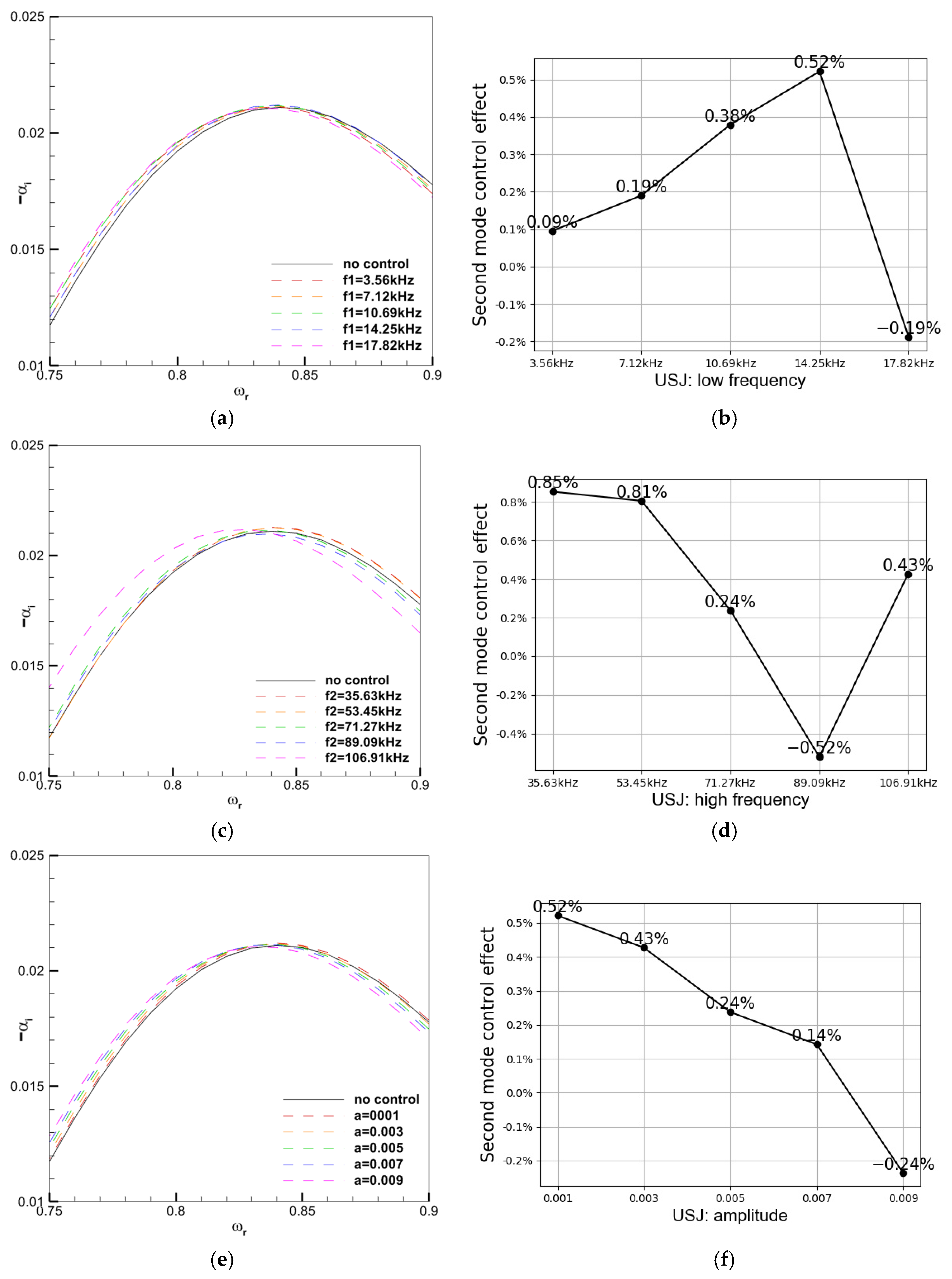
Figure 6 shows the one-way ANOVA results for the second-mode growth rates varying with frequency. For the second mode, only when f₁ = 17.82 kHz, f₂ = 89.9 kHz, a = 0.009, was the growth rate lower than the uncontrolled state, which increased the stability of flow.

3.2. Results of Synthetic Jet Arranged Downstream of Synchronization Point

Table 5. Test results of each case of DSJ.

Case	Maximum Growth Rate		Percentage of Control
	First Mode	Second Mode	First Mode	Second Mode
1	0.00280	0.02117	1.45%	0.43%
2	0.00291	0.02121	5.43%	0.62%
3	0.00287	0.02120	3.99%	0.57%
4	0.00329	0.02128	19.22%	0.95%
5	0.00301	0.02158	9.04%	2.36%
6	0.00290	0.02123	5.15%	0.72%
7	0.00280	0.02117	1.60%	0.43%
8	0.00302	0.02128	9.52%	0.95%
9	0.00308	0.02122	11.52%	0.68%
10	0.00285	0.02126	3.37%	0.85%
11	0.00285	0.02120	3.23%	0.55%
12	0.00301	0.02131	8.94%	1.10%
13	0.00297	0.02128	7.67%	0.94%
14	0.00287	0.02119	4.08%	0.51%
15	0.00311	0.02172	12.72%	3.03%
16	0.00297	0.02128	7.53%	0.94%
17	0.00292	0.02124	5.74%	0.78%
18	0.00283	0.02118	2.54%	0.47%
19	0.00321	0.02124	16.46%	0.77%
20	0.00297	0.02145	7.49%	1.77%
21	0.00291	0.02124	5.29%	0.77%
22	0.00283	0.02119	2.55%	0.51%
23	0.00302	0.02129	9.54%	1.01%
24	0.00298	0.02120	7.95%	0.56%
25	0.00320	0.02185	16.01%	3.67%

is the results of each case of the DSJ. It can be seen that the DSJ plays a role in promoting transition, with the growth rate of all cases being larger than in the uncontrolled state.

Case 4 exhibited the most significant promotional impact on the first mode, achieving a nearly 20% increase. Similarly, case 25 demonstrated the strongest promotional effect on the second mode, with an increase of 3.67%. These findings are represented in Figure 7 below.

Table 6. Results of multivariate variance analysis of the first and second modes of the DSJ.

Source of Variance	p
	First Mode	Second Mode
f1	0.496	0.181
f2	0.0001	0.0002
a	0.0003	0.013

presents the results of the multi-factor variance analysis of the DSJ on the first and second modes. In both modes, the p-value for f₂ and a is less than 0.05, indicating a significant difference [33], whereas the differences observed among f₁ are small.

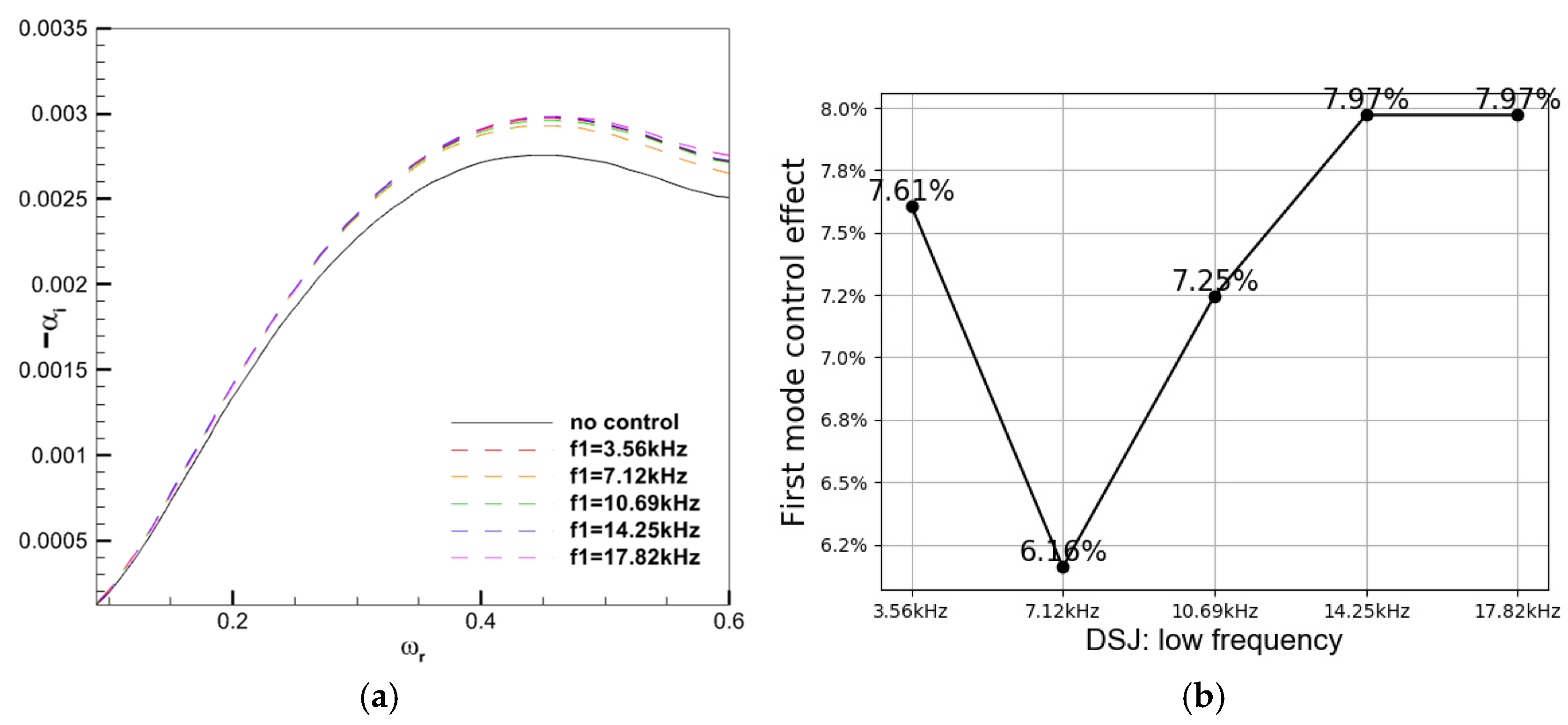
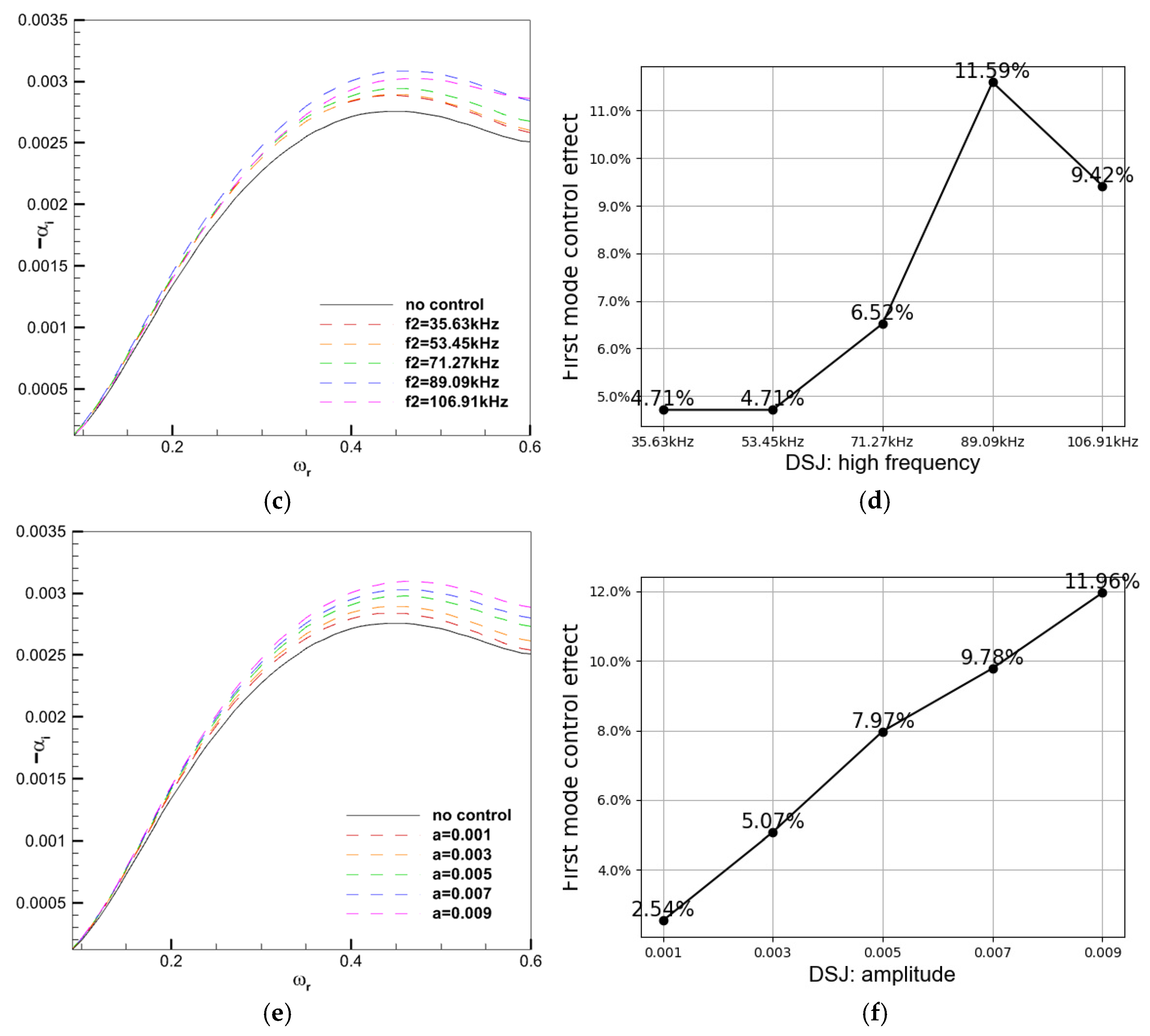
One-way ANOVA was conducted to examine the growth rates of the first mode varying with frequency, controlled by the low frequency, high frequency, and amplitude of the DSJ, as shown in Figure 8. These figures illustrate the control mechanism of the DSJ on the first mode.

At the five levels of f₁, the growth rate was approximately 7% higher compared to the uncontrolled state. As the f₂ increased, the growth rate of the first mode also rose until it reached f₂ = 89.89 kHz. At this point, the promotion effect on the first mode reached its peak at 11.59%, resulting in an earlier transition. Moreover, a larger value of a corresponded to a higher growth rate of the first mode, which also led to increased flow instability.

Figure 9 presents the results of the one-way ANOVA for the growth rates of the second mode in relation to the DSJ. In the case of the second mode, the growth rate was only about 1% higher than that of the uncontrolled state at the five levels of f₁, which is not particularly significant. However, at levels of f₂, the growth rate of the second mode reached as high as 2.28%, resulting in increased flow instability. The influence of parameter a on the control effect was minimal, but the growth rate did increase with higher values of a.

Based on the aforementioned analysis, it is evident that under specific parameters, a USJ can hinder the growth of both the first and second modes, thereby delaying the transition. The case with optimal transition delaying effect was case 4: f₁ = 3.56 kHz, f₂ = 89.9 kHz, a = 0.009, wherein the maximum growth rate of the first mode was reduced by 9.06% and that of the second mode was reduced by 1.28%. On the other hand, the DSJ, regardless of the parameters, increased flow instability and accelerated the transition, with higher frequencies and amplitudes resulting in greater growth rates for both modes. High frequency demonstrated significant differences for both the USJ and DSJ, followed by low frequency and amplitude. The low frequency had a favorable effect on the first mode, whereas the high frequency exhibited a great impact on both first and second modes.

4. Variation in Growth Rate with Spanwise Wave Number

In the previous section, the growth rate variation with frequency ω was examined while the spanwise wave number was kept fixed at β_r = 0. However, this approach did not provide insights into how the growth rate changes with β_r. In this section, we describe our investigation into the relationship between the growth rate and the spanwise wave number for the first mode (ω = 0.45) and second mode (ω = 0.84).

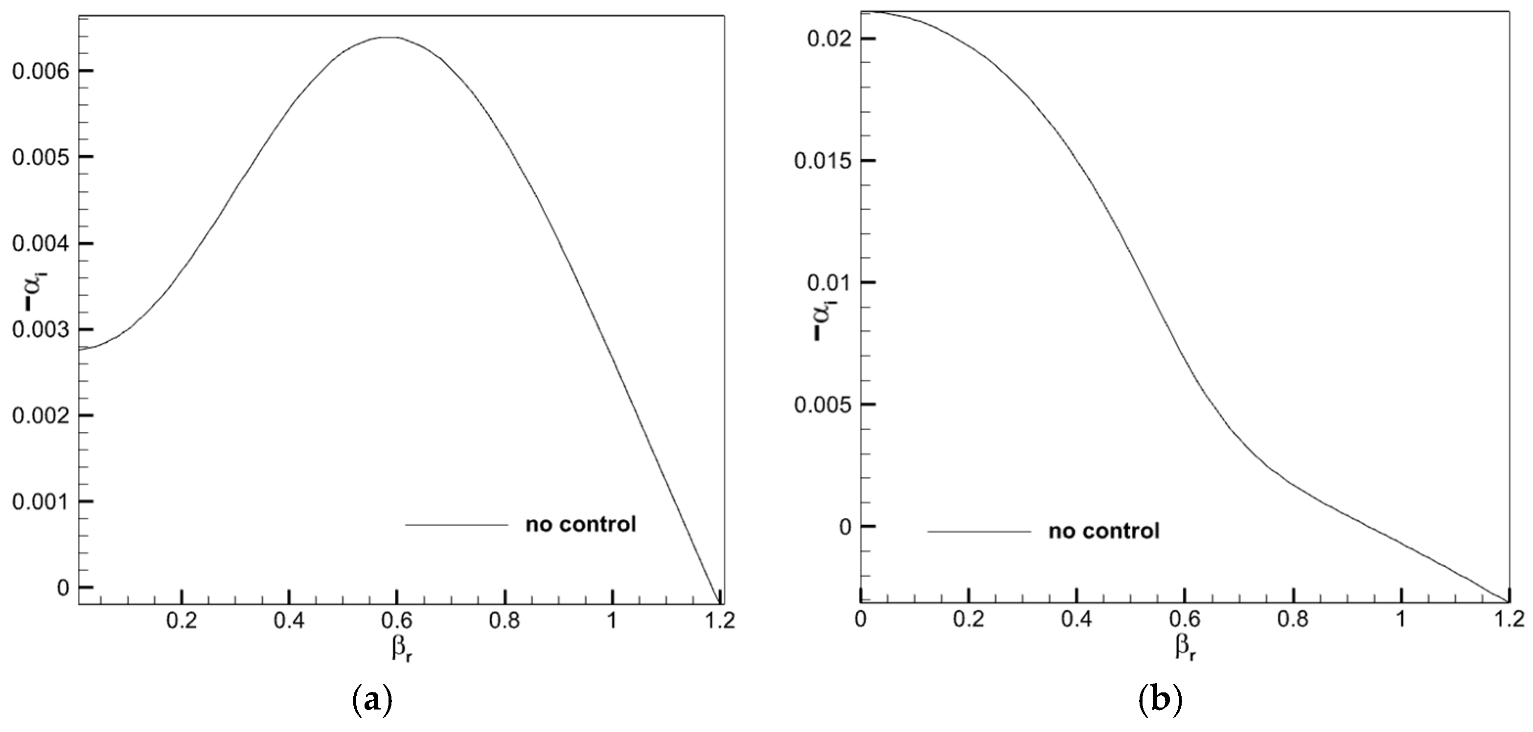
Figure 10 illustrates the first- and second-mode growth rates varying with spanwise wave number β_r in the uncontrolled state. As β_r increased, the growth rate of the first mode gradually rose and reached its peak at approximately 0.0062, whereas the second-mode growth rate gradually decreased. This indicates that the most unstable first mode is the three-dimensional unstable wave, and the most unstable second mode is the two-dimensional wave.

4.1. Results of Synthetic Jet Arranged Upstream of Synchronization Point

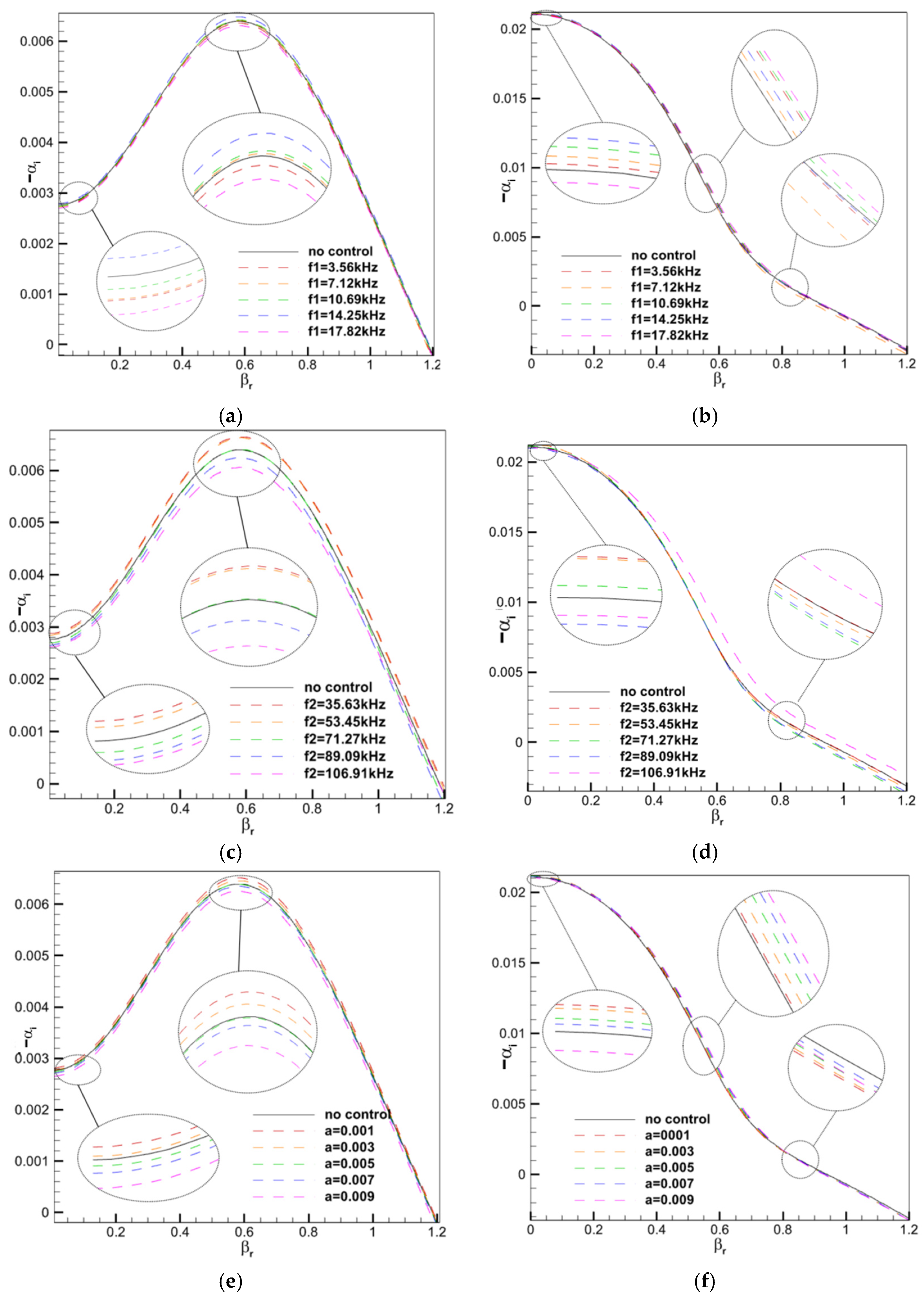
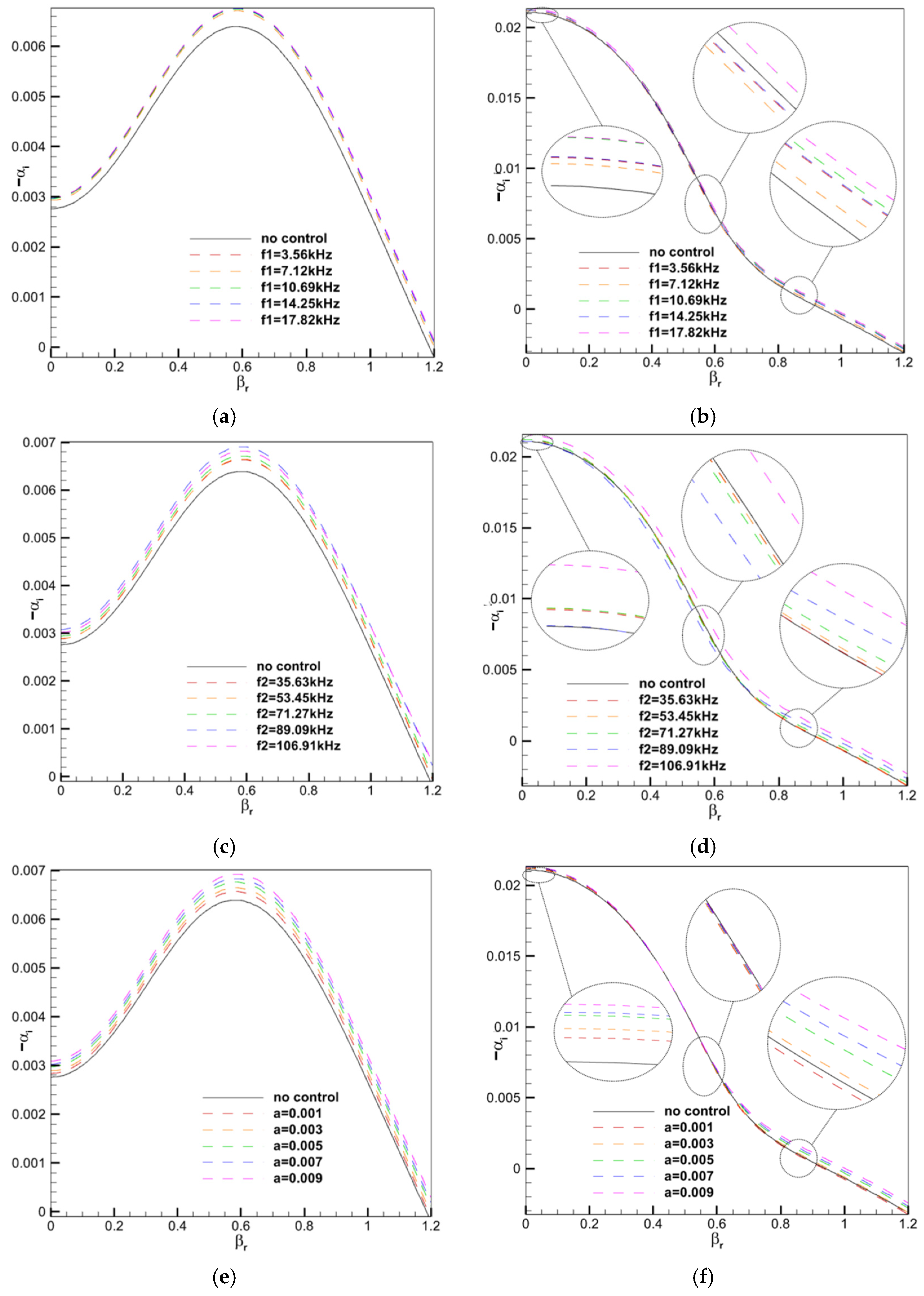
Figure 11 presents the results of the one-way ANOVA conducted for the growth rates of the first and second modes as the spanwise wave number changed, controlled by the low frequency, high frequency, and amplitude of the USJ. The control rule of the parameter varied under different β_r, resulting in a complex pattern. However, it is worth noting that case 4, with f₁ = 3.56 kHz, f₂ = 89.9 kHz, a = 0.009, could effectively reduce the growth rate compared to the uncontrolled state across a wide range of β_r. This demonstrates its potential for inhibiting the transition process.

4.2. Results of Synthetic Jet Arranged Downstream of Synchronization Point

Figure 12 illustrates the results of the one-way ANOVA conducted on the growth rates with varying spanwise wave numbers controlled by the DSJ. The findings reveal that, for the first mode, the control rule remained consistent across all spanwise wave numbers. The growth rate at all levels of frequency and amplitude was higher than in the uncontrolled state, resulting in the promotion of the transition process. On the other hand, for the second mode, a suppressing effect was observed at certain levels under the intermediate spanwise wave number, where the growth rate was lower than in the uncontrolled state.

5. Flow Field Structure Analysis

Pressure disturbance, also known as pressure pulsation, is obtained by subtracting the average flow field pressure from the instantaneous flow field pressure.

$$p^{\prime }(x,y,z,t)=p(x,y,z,t)-\overline{p}(x,y,z,t)$$

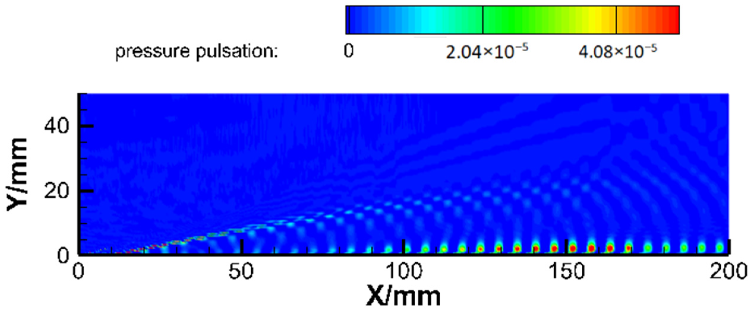
Figure 13 shows the pressure pulsation diagram of the uncontrolled flow field. It is evident that an oblique shock wave forms at the leading edge of the plate, followed by a double cell structure of pressure pulsation, which gradually increases along the boundary layer. This structure intensifies along the boundary layer, with the twin-cell pattern growing and becoming increasingly unstable downstream. As a result, the boundary layer gradually loses stability.

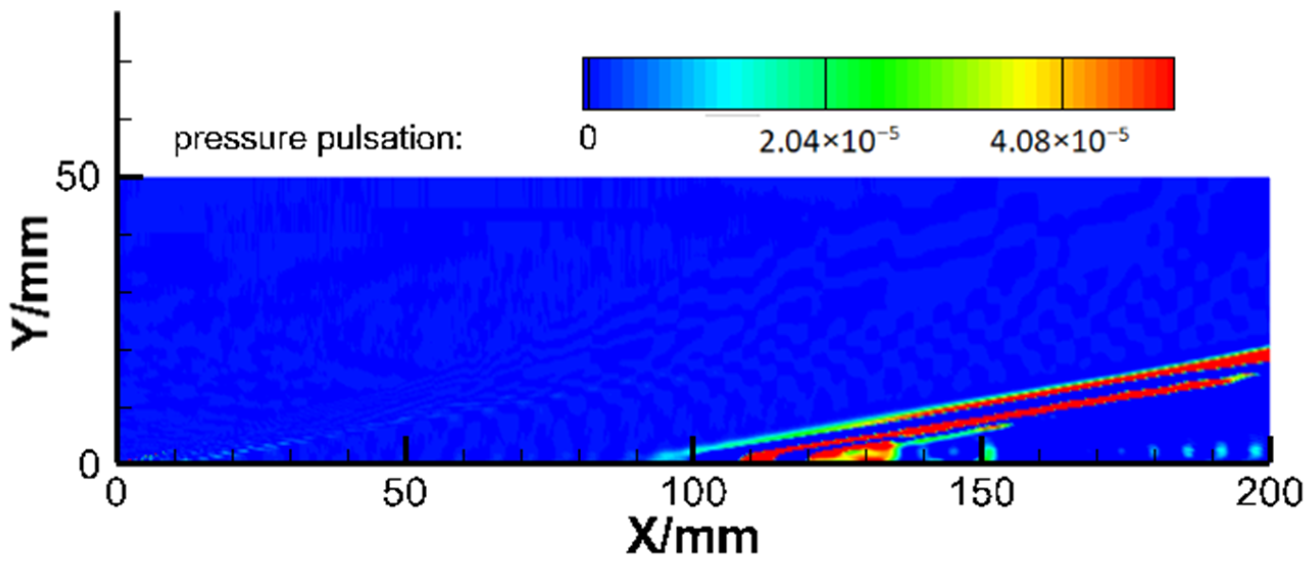
Figure 14 illustrates the pressure pulsation diagram of the flow field with suppressed transition, specifically case 4 of the USJ. Due to the temporal variation of pressure fluctuations, conducting a one-way ANOVA was not convenient. Therefore, only selected experimental groups were analyzed.

It can be observed that the bi-frequency synthetic jet generated weak expansion and compression waves upstream. However, beyond the wave system, the twin-cell structure of pressure pulsation was relatively smaller compared to the uncontrolled state. This indicates that the flow tends to stabilize, leading to the suppression of transition.

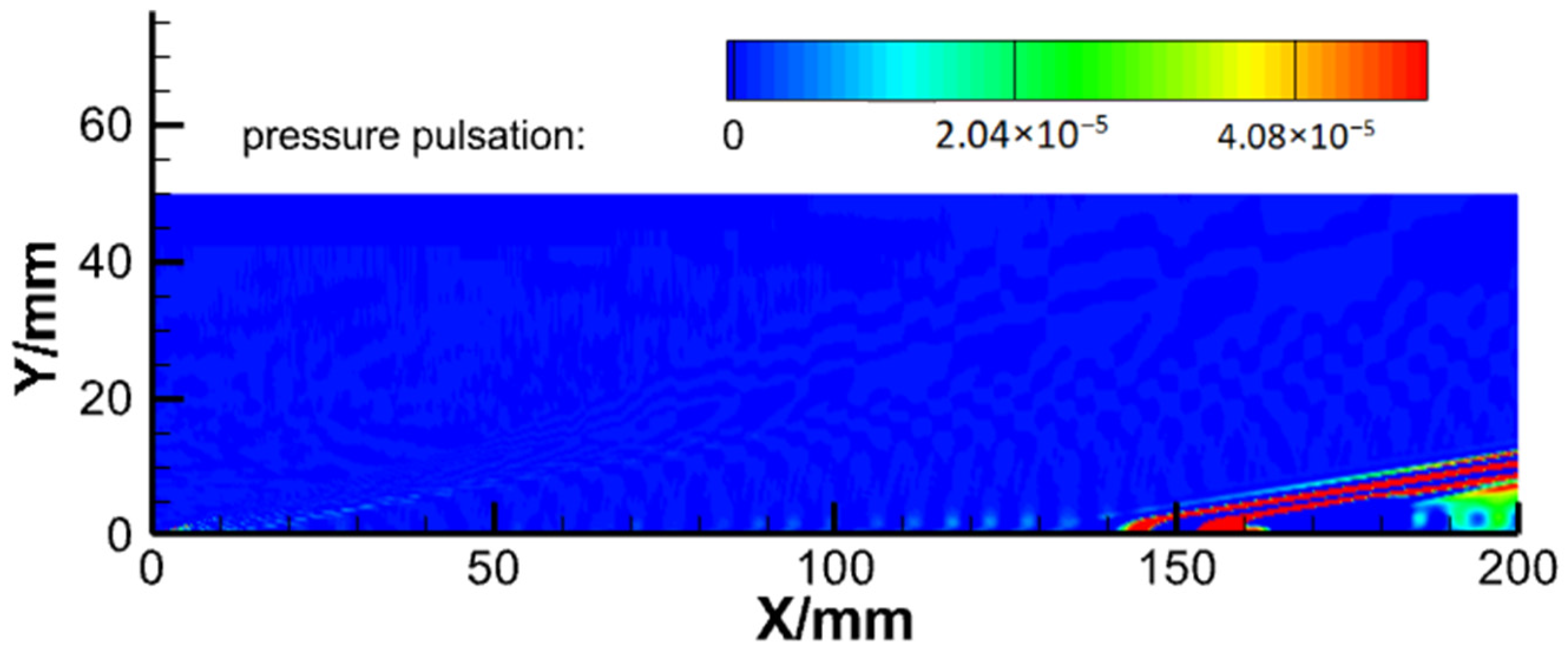
Figure 15 displays the pressure pulsation diagram of the flow field with promoted transition, specifically case 19 of the DSJ. It is evident that beyond the wave system, the twin-cell structure of pressure pulsation further intensified until it merged with the wave system structure, indicating increased flow instability and transition promotion.

6. Disturbance Temperature Eigenfunction Analysis

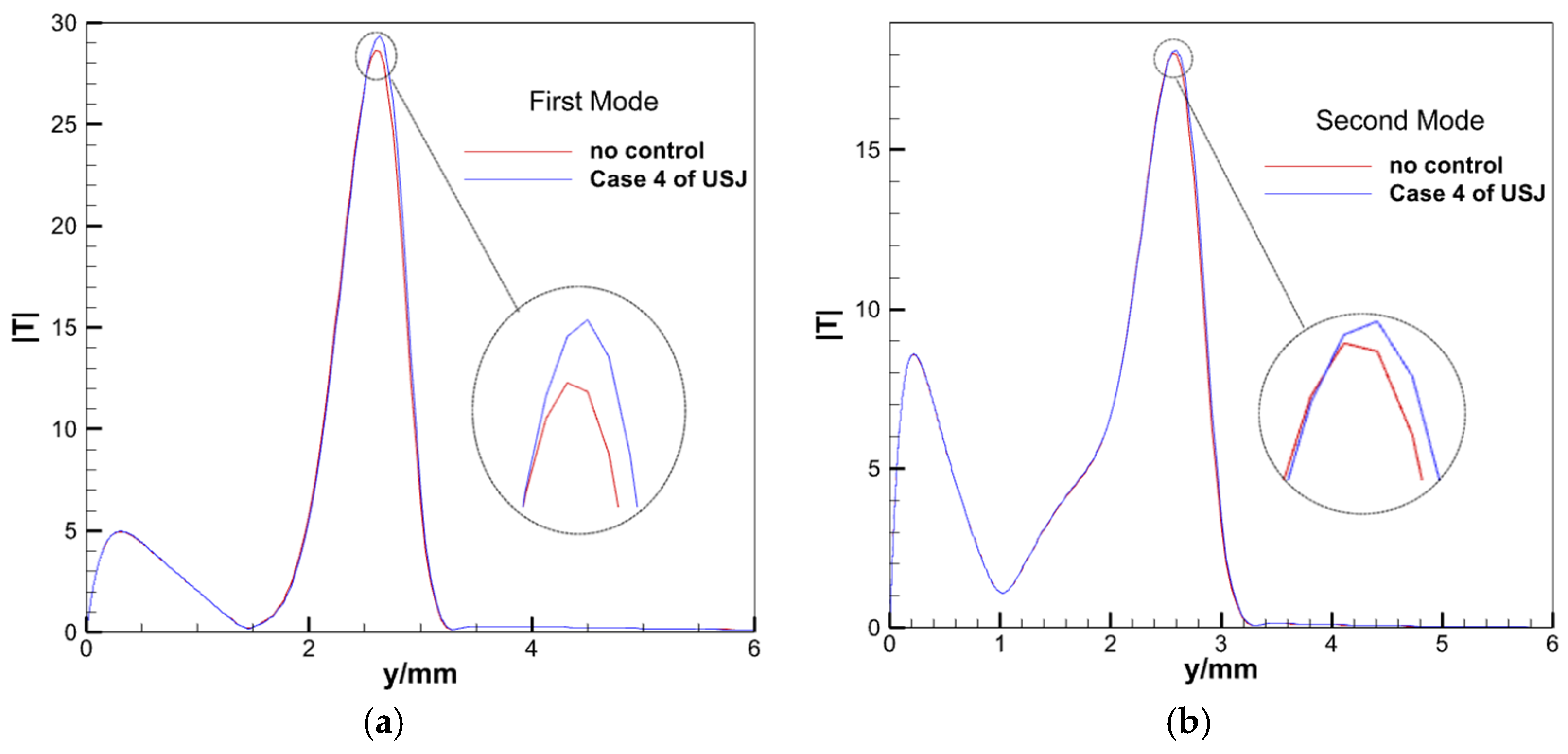
Figure 16 shows the disturbance temperature eigenfunction of case 4 of the USJ, which exhibited the best transition suppression effect. It can be observed that although case 4 has a suppressing effect on both the first and second modes, the peak values of the disturbance temperature eigenfunctions for both modes are larger compared to the uncontrolled state. The suppression effect on the first mode was better than that on the second mode, and the increase in the peak value of the temperature eigenfunction was also greater for the first mode compared to the second mode. This phenomenon has also been observed in the study by Liu [29] on synthetic jets and wall blowing/suction for transition control. This finding suggests that the suppression of unstable modes may be achieved through temperature modification. Arthur Poulain [36] pointed out that the control mechanism of wall blowing/suction for transition is its modification of the momentum in the boundary layer. The temperature modification discovered in this study may be related to the velocity–temperature coupling mechanism in hypersonic flows.

7. Conclusions

This paper proposes a novel transition-delaying control method of hypersonic boundary layer transition based on a bi-frequency synthetic jet. Orthogonal table and multi-factor/one-way ANOVA were used to study the control effects of the three parameters of the bi-frequency synthetic jet located in the upstream and downstream of the synchronization point. Effects were studied of low frequency, high frequency and amplitude on the growth rates of unstable modes, and are reflected in the change in the growth rate with frequency and the change in the growth rate with the spanwise wave number. Linear stability theory was adopted to analyze the control effect.

In terms of the growth rate varying with frequency, results show that a USJ can hinder the growth of both the first and second modes under specific parameters, thereby delaying the transition, whereas a DSJ increases flow instability and accelerates the transition regardless of frequency or amplitude. For the low frequency, high frequency and amplitude of a USJ, specific levels of f₁ can suppress the first mode. The higher the f₂ was, the lower was the growth rate of the first mode, with the suppression effect limited to f₂ = 89.09 kHz for the second mode. Increasing a led to a lower growth rate for both the first and second modes, resulting in a more pronounced suppression effect. Conversely, for f₁, f₂, a of the DSJ, as the levels of these three parameters increased, the growth rate of unstable modes also increased, leading to an increase in flow instability. In terms of the growth rate varying with the spanwise wave number, the control rule of the same parameter varied under different β_r, resulting in a complex pattern.

The optimal delay effect on transition is case 4 of the USJ, with f₁ = 3.56 kHz, f₂ = 89.9 kHz, a = 0.009, so that the maximum growth rate of the first mode was reduced by 9.06% and that of the second mode was reduced by 1.28% compared with the uncontrolled state. Also, the low-field analysis reveals a weakening of the twin lattice structure of pressure pulsation, thus improving the stability of the flow.

References

- Liu, Q.; Luo, Z.; Wang, L.; Tu, G.; Deng, X.; Zhou, Y. Direct numerical simulations of supersonic turbulent boundary layer with streamwise-striped wall blowing. Aerosp. Sci. Technol. 2021, 110, 106510. [Google Scholar] [CrossRef]
- Fedorov, A. Transition and stability of high-speed boundary layers. Annu. Rev. Fluid Mech. 2011, 43, 79–95. [Google Scholar] [CrossRef]
- Kachanov, Y.S. Physical mechanisms of laminar-boundary-layer transition. Annu. Rev. Fluid Mech. 1994, 26, 411–482. [Google Scholar] [CrossRef]
- Yanbao, M.; Xiaolin, Z. Receptivity of a supersonic boundary layer over a flat plate. Part 1. Wave structures and interaction. J. Fluid Mech. 2003, 488, 31–78. [Google Scholar]
- Craig, S.A.; Humble, R.A.; Hofferth, J.W.; Saric, W.S. Nonlinear behavior of the Mack mode in a hypersonic boundary layer. J. Fluid Mech. 2019, 872, 74–99. [Google Scholar] [CrossRef]
- Zhong, X.; Wang, X. Direct numerical simulation on the receptivity, instability, and transition of hypersonic boundary layers. Annu. Rev. Fluid Mech. 2012, 44, 527–561. [Google Scholar] [CrossRef]
- Mack, L.M. Computational of the stability of the laminar compressible boundary layers. Methods Comput. Phys. 1965, 4, 247–299. [Google Scholar]
- Zurigat, Y.H.; Nayfeh, A.H.; Masad, J.A. Effect of pressure gradient on the stability of compressible boundary layers. AIAA J. 1992, 30, 2204–2211. [Google Scholar] [CrossRef]
- Malik, M.R. Prediction and control of transition in supersonic and hypersonic boundary layers. AIAA J. 1989, 27, 1487–1493. [Google Scholar] [CrossRef]
- Kimmel, R.L.; Poffie, J. Effect of Total Temperature on Boundary Layer Stability at Mach 6; AIAA: Reston, VA, USA, 1999; pp. 1–2, 1999–0816. [Google Scholar]
- Paredes, P.; Choudhari, M.M.; Li, F. Transition delay via vortex generators in a hypersonic boundary layer at flight conditions. In Proceedings of the 2018 Fluid Dynamics Conference, Atlanta, GA, USA, 25–29 June 2018. [Google Scholar]
- Igarashi, T.; Iida, Y. Fluid flow and heat transfer around a circular cylinder with vortex generators. Trans. Jpn. Soc. Mech. Eng. Part B 1985, 51, 2420–2427. [Google Scholar] [CrossRef]
- Schneider, S.P. Effects of roughness on hypersonic boundary-layer transition. J. Spacecr. Rocket. 2008, 45, 193–209. [Google Scholar] [CrossRef]
- Fedorov, A. Receptivity of Hypersonic Boundary Layer to Acoustic Disturbances Scattered by Surface Roughness; AIAA: Reston, VA, USA, 2003; pp. 1–3, 2003–3731. [Google Scholar]
- Schneider, S.P. Summary of hypersonic boundary-layer transition experiments on blunt bodies with roughness. J. Spacecr. Rocket. 2008, 45, 1090–1105. [Google Scholar] [CrossRef]
- Liu, X.; Yi, S.; Xu, X.; Shi, Y.; Ouyang, T.; Xiong, H. Experimental study of second-mode wave on a flared cone at Mach 6. Phys. Fluids 2019, 31, 074108. [Google Scholar] [CrossRef]
- Fujii, K. Experiment of the two-dimensional roughness effect on hypersonic boundary-layer transition. J. Spacecr. Rocket. 2006, 43, 731–738. [Google Scholar] [CrossRef]
- Gaponov, S.A.; Terekhova, N.M. Stability of supersonic boundary layer on a porous plate with a flexible coating. Thermophys. Aeromechanics 2014, 21, 143–156. [Google Scholar] [CrossRef]
- Morozov, S.O.; Lukashevich, S.V.; Soudakov, V.G.; Shiplyuk, A.N. Experimental study of the influence of small angles of attack and cone nose bluntness on the stabilization of hypersonic boundary layer with passive porous coating. Thermophys. Aeromechanics 2018, 25, 793–800. [Google Scholar] [CrossRef]
- Gaponov, S.A.; Ermolaev, Y.G.; Kosinov, A.D.; Lysenko, V.I.; Semenov, N.V.; Smorodskii, B.V. Influence of porous-coating thickness on the stability and transition of flat-plate supersonic boundary layer. Thermophys. Aeromechanics 2012, 19, 555–560. [Google Scholar] [CrossRef]
- Germain, P.D.; Hornung, H.G. Transition on a slender cone in hypervelocity flow. Exp. Fluids 1997, 22, 183–190. [Google Scholar] [CrossRef]
- Gaponov, S.A.; Smorodsky, B.V. Control of supersonic boundary layer and its stability by means of foreign gas injection through the porous wall. Int. J. Theor. Appl. Mech. 2016, 1, 97–103. [Google Scholar]
- Miró, F.; Pinna, F. Injection-gas-composition effects on hypersonic boundary-layer transition. J. Fluid Mech. 2020, 890, R4. [Google Scholar] [CrossRef]
- Orlik, E.; Fedioun, I.; Lardjane, N. Hypersonic boundary-layer transition forced by wall injection: A numerical study. J. Spacecr. Rocket. 2014, 51, 1306–1318. [Google Scholar] [CrossRef]
- Liu, Q.; Luo, Z.; Deng, X.; Yang, S.; Jiang, H. Linear stability of supersonic boundary layer with synthetic cold/hot jet control. Acta Phys. Sin. 2017, 66, 222–232. [Google Scholar]
- Brett, F.B.; Paul, M.D.; Jennifer, A.I.; David, W.A.; Scott, A.B. PLIF Visualization of Active Control of Hypersonic Boundary Layers Using Blowing; AIAA Paper; AIAA: Reston, VA, USA, 2008; pp. 1–2, 2008–4266. [Google Scholar]
- Rui, Z.; Chiyong, W.; Xudong, T.; Tiehan, L. Numerical simulation of local wall heating and cooling effect on the stability of a hypersonic boundary layer. Int. J. Heat Mass Transf. 2018, 121, 986–998. [Google Scholar]
- Unnikrishnan, S.; Gaitonde, D.V. Instabilities and transition in cooled wall hypersonic boundary layers. J. Fluid Mech. 2021, 915, A26. [Google Scholar] [CrossRef]
- Liu, Q. Research on Control Methods and Mechanisms of Supersonic/Hypersonic Boundary Layer Drag Reduction Subject to Active Flow Control. Ph.D. Thesis, National University of Defense Technology, Changsha, China, 2021. [Google Scholar]
- Li, X.; Fu, D.; Ma, Y.; Liang, X. Direct numerical simulation of compressible turbulent flows. Acta Mech. Sin. 2010, 26, 795–806. [Google Scholar] [CrossRef]
- Zhou, B.; Qu, F.; Liu, Q.; Sun, D.; Bai, J. A study of multidimensional fifth-order WENO method for genuinely two-dimensional Riemann solver. J. Comput. Phys. 2022, 463, 111249. [Google Scholar] [CrossRef]
- Chen, S.-S.; Cai, F.-J.; Xue, H.-C.; Wang, N.; Yan, C. An improved AUSM-family scheme with robustness and accuracy for all Mach number flows. Appl. Math. Model. 2020, 77, 1065–1081. [Google Scholar] [CrossRef]
- Clarke, G.M. Introduction to the Design and Analysis of Experiments; Wiley: Hoboken, NJ, USA, 1996. [Google Scholar]
- Heisenberg, W. Uber stabilitat und turbulenz von flussigkeits-stommen. Annu. Phys. 1924, 74, 577–627. [Google Scholar] [CrossRef]
- Malik, M.R. Numerical methods for hypersonic boundary layer stability. J. Comput. Phys. 1990, 86, 376–413. [Google Scholar] [CrossRef]
- Poulain, A.; Content, C.; Rigas, G.; Garnier, E.; Sipp, D. Adjoint-based linear sensitivity of a hypersonic boundary layer to steady wall blowing-suction/heating-cooling. J. Fluid Mech. 2023. [Google Scholar]
Figure 1.
Schematic model of flat plate with disturbance and control.
Figure 2.
Grid of the flow field.
Figure 3.
Growth rate varying with frequency in uncontrolled state.
Figure 4.
Growth rate varying with frequency in cases 4, 15 and 16 of USJ.
Figure 5.
One-way ANOVA for the first-mode growth rates varying with frequency, controlled by the low frequency, high frequency and amplitude of USJ. (a) First-mode growth rate varying with frequency, controlled by the low frequency of USJ. (b) First-mode maximum growth rate varying with low frequency of USJ. (c) First-mode growth rate varying with frequency, controlled by the high frequency of USJ. (d) First-mode maximum growth rate varying with high frequency of USJ. (e) First-mode growth rate varying with frequency, controlled by the amplitude of USJ. (f) First-mode maximum growth rate varying with amplitude of USJ.
Figure 6.
One-way ANOVA for the second-mode growth rates varying with frequency, controlled by the low frequency, high frequency and amplitude of USJ. (a) Second-mode growth rate varying with frequency, controlled by the low frequency of USJ. (b) Second-mode maximum growth rate varying with low frequency of USJ. (c) Second-mode growth rate varying with frequency, controlled by the high frequency of USJ. (d) Second-mode maximum growth rate varying with high frequency of USJ. (e) Second-mode growth rate varying with frequency, controlled by the amplitude of USJ. (f) Second-mode maximum growth rate varying with amplitude of USJ.
Figure 7.
Growth rate varying with frequency of cases 4 and 25 of DSJ.
Figure 8.
One-way ANOVA for the first-mode growth rates varying with frequency, controlled by the low frequency, high frequency and amplitude of DSJ. (a) First-mode growth rate varying with frequency, controlled by the low frequency of DSJ. (b) First-mode maximum growth rate varying with low frequency of DSJ. (c) First-mode growth rate varying with frequency, controlled by the high frequency of DSJ. (d) First-mode maximum growth rate varying with high frequency of DSJ. (e) First-mode growth rate varying with frequency, controlled by the amplitude of DSJ. (f) First-mode maximum growth rate varying with amplitude of DSJ.
Figure 9.
One-way ANOVA for the second-mode growth rates varying with frequency, controlled by the low frequency, high frequency and amplitude of DSJ. (a) Second-mode growth rate varying with frequency, controlled by the low frequency of DSJ. (b) Second-mode maximum growth rate varying with low frequency of DSJ. (c) Second-mode growth rate varying with frequency, controlled by the high frequency of DSJ. (d) Second-mode maximum growth rate varying with high frequency of DSJ. (e) Second-mode growth rate varying with frequency, controlled by the amplitude of DSJ. (f) Second-mode maximum growth rate varying with amplitude of DSJ.
Figure 10.
First- and second-mode growth rates varying with the spanwise wave number in the uncontrolled case. (a) First-mode growth rate varying with spanwise wave number in the uncontrolled state. (b) Second-mode growth rate varying with spanwise wave number in the uncontrolled state.
Figure 11.
The first- and second-mode growth rates varying with spanwise wave number, controlled by the low frequency, high frequency and amplitude of USJ. (a) The first-mode growth rate varying with spanwise wave number, controlled by the low frequency of USJ. (b) The second-mode growth rate varying with spanwise wave number, controlled by the low frequency of USJ. (c) The first-mode growth rate varying with spanwise wave number, controlled by the high frequency of USJ. (d) The second-mode growth rate varying with spanwise wave number, controlled by the high frequency of USJ. (e) The first-mode growth rate varying with spanwise wave number, controlled by the amplitude of USJ. (f) The second-mode growth rate varying with spanwise wave number, controlled by the amplitude of USJ.
Figure 12.
The first- and second-mode growth rates varying with spanwise wave number, controlled by the low frequency, high frequency and amplitude of DSJ. (a) The first-mode growth rate varying with spanwise wave number, controlled by the low frequency of DSJ. (b) The second-mode growth rate varying with spanwise wave number, controlled by the low frequency of DSJ. (c) The first-mode growth rate varying with spanwise wave number, controlled by the high frequency of DSJ. (d) The second-mode growth rate varying with spanwise wave number, controlled by the high frequency of DSJ. (e) The first-mode growth rate varying with spanwise wave number, controlled by the amplitude of DSJ. (f) The second-mode growth rate varying with spanwise wave number, controlled by the amplitude of DSJ.
Figure 13.
Pressure pulsation diagram in uncontrolled state.
Figure 14.
Pressure pulsation diagram with transition suppressed.
Figure 15.
Pressure pulsation diagram with transition promoted.
Figure 16.
Pressure pulsation diagram with transition promoted. (a) The disturbance temperature eigenfunction of the first mode. (b) The disturbance temperature eigenfunction of the second mode.