
Parameter-Free Shape Optimization: Various Shape Updates for Engineering Applications
by
 , , , , , and
Lars Radtke
1,*,
Georgios Bletsos
2,
Niklas Kühl
2,
Tim Suchan
3,
Thomas Rung
2,
Alexander Düster
1 and
Kathrin Welker
4 1
Institute for Ship Structural Design and Analysis (M-10), Numerical Structural Analysis with Application in Ship Technology, Hamburg University of Technology, 21073 Hamburg, Germany
2
Institute for Fluid Dynamics and Ship Theory (M-8), Hamburg University of Technology, 21073 Hamburg, Germany
3
Faculty for Mechanical and Civil Engineering, Helmut Schmidt University, 22008 Hamburg, Germany
4
Institute of Numerical Mathematics and Optimization, Technische Universität Bergakademie Freiberg, 09599 Freiberg, Germany
*
Author to whom correspondence should be addressed.
Aerospace 2023, 10(9), 751; https://doi.org/10.3390/aerospace10090751
Submission received: 29 June 2023
/
Revised: 11 August 2023
/
Accepted: 18 August 2023
/
Published: 25 August 2023
(This article belongs to the Special Issue Adjoint Method for Aerodynamic Design and Other Applications in CFD)
Abstract
:In the last decade, parameter-free approaches to shape optimization problems have matured to a state where they provide a versatile tool for complex engineering applications. However, sensitivity distributions obtained from shape derivatives in this context cannot be directly used as a shape update in gradient-based optimization strategies. Instead, an auxiliary problem has to be solved to obtain a gradient from the sensitivity. While several choices for these auxiliary problems were investigated mathematically, the complexity of the concepts behind their derivation has often prevented their application in engineering. This work aims to explain several approaches to compute shape updates from an engineering perspective. We introduce the corresponding auxiliary problems in a formal way and compare the choices by means of numerical examples. To this end, a test case and exemplary applications from computational fluid dynamics are considered.
1. Introduction
Shape optimization is a broad topic with many applications and a large variety of methods. This paper focuses on gradient-based shape optimization methods designed to solve problems that are constrained by partial differential equations (PDE). These arise, for example, in many fields of engineering such as fluid mechanics [1,2,3], structural mechanics [4,5] and acoustics [6,7]. Since they may be trapped in a local optimum, gradient-descent methods are favorable in globally convex optimization problems or when an improved configuration is sought based on an already existing design. The latter is frequently the case in many engineering-scale applications, in which the initial design usually corresponds to an existing model that is already functional. However, in cases where a numerical estimation of the gradient is either insufficient or impractical to obtain, a promising alternative can be found in gradient-free methods. For a detailed discussion of these methods, we refer the reader to [8,9].
In order to computationally solve a PDE constraint of an optimization problem, the domain under investigation needs to be discretized, i.e., a computational mesh is required. In this paper, we are particularly concerned with boundary-fitted meshes and methods, where shape updates are realized through updates of the mesh. However, it is worth mentioning that alternatives to mesh morphing-based methods, such as immersed boundary or level-set methods, have been investigated in the context of shape or predominantly topology optimization [10,11]. However, additional analytic effort is required to differentiate the adjoint method up to the immersed boundary representation. Moreover, it is well known that in level-set approaches an adaptive concept for the spatial resolution is indispensable.
In the context of boundary-fitted meshes, solution methods for gradient-based shape optimization problems may be loosely divided into parameterized and parameter-free approaches. With parameterized, we refer to methods that describe the shape through a finite number of parameters. The parameterization is prescribed beforehand and is part of the derivation process of suitable shape updates, see, e.g., [12]. Parameter-free refers to methods that are derived on the continuous level independently of a parameterization. Of course, in an application scenario, also parameter-free approaches finally discretize the shape using the mesh needed for the solution of the PDE.
In general, optimization methods for PDE-constrained problems aim to minimize (or maximize) of an objective functional that depends on the solution (also called the state) of the PDE, e.g., the compliance of an elastic structure [4] or dissipated power in a viscous flow [2]. Since a maximization problem can be expressed as a minimization problem by considering the negative objective functional, we only consider minimization problems in this paper. An in-depth introduction is given in [13]. In this paper, we are concerned with iterative methods that generate shape updates such that the objective functional is reduced. In order to determine suitable shape updates, the so-called shape derivative of the objective functional is utilized. Typically, adjoint methods are used to compute shape derivatives, when the number of design variables is high. This is the case in particular for parameter-free shape optimization approaches, where shapes are not explicitly parameterized (e.g., by splines) and after a final discretization, the number of design variables typically corresponds to the number of nodes in the mesh that is used to solve the constraining PDE. Adjoint methods are favorable in this scenario, because their computational cost to obtain the shape derivative is independent of the number of design variables. For every objective functional, only a single additional problem, the adjoint problem, needs to be derived and solved to obtain the shape derivative. For a general introduction to the adjoint method, we refer the reader to [14,15].
Despite the merits of the adjoint methods in the context of efficiently obtaining a shape derivative, there are also shortcomings. For example, in unsteady problems the complete time history of the primal problem is required since the adjoint problem depends on it in each timestep. This creates high memory demands for engineering-scale applications. However, several techniques have been successfully utilized to overcome this drawback. This includes check-pointing strategies, where the primal solution is stored only at a number of optimally placed check-points in time, see, e.g., [16,17]. Further, compression strategies have been employed to minimize the memory footprint of storing the complete time history. These strategies are usually classified as lossy or non-lossy depending on whether the exact solution can be reconstructed from the compressed data or not, respectively [18]. Furthermore, several problems require the optimization of more than one objective functional. While the adjoint method is most prominent for computing the derivative of a single objective with respect to the control, it can also be utilized for the optimization of multiple objective functionals. In such a case, a usual practice is to define a single objective functional as the weighted sum of the individual quantities of interest. This technique has also been used in conjunction with adjoint methods for robust optimization problems, in which the minimization of the statistical moments of a quantity of interest is desired, see, e.g., [19,20].
In the continuous adjoint method, the shape derivative is usually obtained as an integral expression over the design boundary identified with the shape and gives rise to a scalar distribution over the boundary, the sensitivity distribution, which is expressed in terms of the solution of the adjoint problem. As an alternative to the continuous adjoint method, the discrete adjoint method may be employed. It directly provides sensitivities at discrete points, likely nodes of the computational mesh. A summary of the continuous and the discrete adjoint approach is given in [21].
Especially in combination with continuous adjoint approaches, it is not common to use the derived expression for the sensitivity directly as a shape update within the optimization loop. Instead, sensitivities are usually smoothed or filtered [22]. A focus of this work lies in the explanation of several approaches to achieve this in such a way that they can be readily applied in the context of engineering applications. To this end, we concentrate on questions such as How to apply an approach? and What are the benefits and costs? rather than How can approaches of this type be derived?
Nevertheless, we would like to point out that there is a large amount of literature concerned with the mathematical foundation of shape optimization. For a deeper introduction, one may consult standard textbooks, such as [23,24]. More recently, an in-depth overview on state-of-the-art concepts has been given in [25], including many references. We include Sobolev gradients in our studies, which can be seen as a well-established concept that is applied in many studies to obtain a so-called descent direction (which leads to the shape update) from a shape derivative, see, e.g., [26,27] for engineering and [28,29,30] for mathematical studies. We also look at more recently developed approaches such as the Steklov–Poincaré approach developed in [31] and further investigated in [30] and the p-harmonic descent approach, which was proposed in [32] and further investigated in [33]. In addition, we address discrete filtering approaches, as used, e.g., in [22,34], in our studies.
The considered shape updates have to perform well in terms of mesh distortion. Over the course of the optimization algorithm, the mesh has to be updated several times, including the position of the nodes in the domain interior. The deterioration of mesh quality, especially if large steps are taken in a given direction, is a severe issue that is the subject of several works, see, e.g., [34,35], and plays a major role in the present study as well. Using an illustrative example and an application from computational fluid dynamics (CFD), the different approaches are compared and investigated. However, we do not extensively discuss the derivation of the respective adjoint problem or the numerical solution of the primal and the adjoint problem but refer to the available literature on this topic, see, e.g., [1,2,36,37,38,39,40]. Instead, we focus on the performance of the different investigated approaches, which compute a suitable shape update from a given sensitivity.
The remainder of this paper is structured as follows. In Section 2, we explain the shape optimization approaches from a mathematical perspective and provide some glimpses of the mathematical concepts behind the approaches. This includes an introduction to the concept of shape spaces, and the definition of metrics on tangent spaces that lead to the well-known Hilbertian approaches or Sobolev gradients. These concepts are then applied in Section 3 to formulate shape updates that reduce an objective functional. In Section 4, we apply the various approaches to obtain shape updates in the scope of an illustrative example, which is not constrained by a PDE. This outlines the different properties of the approaches, e.g., their convergence behavior under mesh refinement. In Section 5, a PDE-constrained optimization problem is considered. In particular, the energy dissipation for a laminar flow around a two-dimensional obstacle and in a three-dimensional duct is minimized. The different approaches to compute a shape update are investigated and compared in terms of applicability (in the sense of being able to yield good mesh qualities ) and efficiency (in the sense of yielding fast convergence).
2. Shape Spaces, Metrics and Gradients
This section focuses on the mathematical background behind parameter-free shape optimization and aims to introduce the required terminology and definitions for Section 3, which primarily focuses on straightforward application. However, we will refer back to the mathematical section several times, since some information in Section 3 may be difficult to understand without the mathematical background. In general, we follow the explanations in [41,42], to which we also refer for further reading. And for application to shape optimization, we refer to [25,29,43].
2.1. Definition of Shapes
To enable a theoretical investigation of gradient descent algorithms, we first need to define what we describe as a shape. There are multiple options, e.g., the usage of landmark vectors [44,45,46,47,48], plane curves [49,50,51,52] or surfaces [53,54,55,56,57] in higher dimensions, boundary contours of objects [58,59,60], multiphase objects [61], characteristic functions of measurable sets [62] and morphologies of images [63]. For our investigations in a two-dimensional setting, we will describe the shape as a plane curve embedded in the surrounding two-dimensional space, the so-called hold-all domain similar to [64], and for three-dimensional models, we use a two-dimensional surface embedded in the surrounding three-dimensional space . Additionally, we need the definition of a Lipschitz shape, which is a curve embedded in or a surface embedded in that can be described by (a graph of) a Lipschitz-continuous function. Furthermore, we define a Lipschitz domain as a domain that has a Lipschitz shape as boundary. The concept of smoothness of shapes in two dimensions is sketched in Figure 1.
2.2. The Concept of Shape Spaces
The definition of a shape space, i.e., a space of all possible shapes, is required for theoretical investigations of shape optimization. Since we focus on gradient descent algorithms, the possibility to use these algorithms requires the existence of gradients. Gradients are trivially computed in Euclidean space (e.g., , ); however, shape spaces usually do not have a vector space structure. Instead, the next-best option is to aim for a manifold structure with an associated Riemannian metric, a so-called Riemannian manifold.
A finite-dimensional manifold is a topological space and additionally fulfills the three conditions.
- 1.
- Locally, it can be described by a Euclidean space.
- 2.
- It can completely be described by countably many subsets (second axiom of countability).
- 3.
- Different points in the space have different neighborhoods (Hausdorff space).
If the subsets, so-called charts, are compatible, i.e., there are differentiable transitions between charts, then the manifold is a differentiable manifold and allows the definition of tangent spaces and directions, which are paramount for further analysis in the field of shape optimization. The tangent space at a point on the manifold is a space tangential to the manifold and describes all directions in which the point could move. It is of the same dimension as the manifold. If the transition between charts is infinitely smooth, then we call the manifold a smooth manifold.
Extending the previous definition of a finite-dimensional manifold into infinite dimensions while dropping the second axiom of countability and Hausdorff yields infinite-dimensional manifolds. A brief introduction and overview about concepts for infinite-dimensional manifolds is given in ([29] Section 2.3), and the references therein.
In case a manifold structure cannot be established for the shape space in question, an alternative option is a diffeological space structure. These describe a generalization of manifolds, i.e., any previously mentioned manifold is also a diffeological space. Here, the subsets to completely parametrize the space are called plots. As explained in [65], these plots do not necessarily have to be of the same dimension as the underlying diffeological space and the mappings between plots do not necessarily have to be reversible. In contrast to shape spaces as Riemannian manifolds, research for diffeological spaces as shape spaces has just begun, see, e.g., [30,66]. Therefore, for the following section, we focus on Riemannian manifolds first and then briefly consider diffeological spaces.
2.3. Metrics on Shape Spaces
In order to define distances and angles on the shape space, a metric on the shape space is required. Distances between iterates (in our setting, shapes) are necessary, e.g., to state convergence properties or to formulate appropriate stopping criteria of optimization algorithms. For all points m on the manifold M, a Riemannian metric defines a positive definite inner product on the tangent space at each . If the inner product is not positive definite but at least non-degenerate as defined in, e.g., ([67], Definition 8.6),then we call the me tric a pseudo-Riemannian metric. This yields a family of inner products such that we have a positive definite inner product available at any point of the manifold. Additionally, it also defines a norm on the tangent space at m as . If such a Riemannian metric exists, then we call the differentiable manifold a Riemannian manifold, often denoted as .
Different types of metrics on shape spaces can be identified, e.g., inner metrics [50,53,54], outer metrics [46,50,68,69,70], metamorphosis metrics [71,72], the Wasserstein or Monge–Kantorovic metric for probability measures [73,74,75], the Weil–Peterson metric [76,77], current metrics [78,79,80] and metrics based on elastic deformations [58,81].
To obtain a metric in the classical sense, we also need a definition of distance in addition to the Riemannian metric. Following [29,42,43], to obtain an expression for distances on the manifold, we first define the length of a differentiable curve on the manifold starting at m using the Riemannian metric as
and then define the distance function as the infimum of any curve length that starts at and ends at , i.e.,
This distance function is called the Riemannian distance or geodesic distance, since the so-called geodesic describes the shortest distance between two points on the manifold. For more details about geodesics, we refer to [82].
If one were able to obtain the geodesic, then a local mapping from the tangent space to the manifold would already be available: the so-called exponential map. However, finding the exponential map requires the solution of a second-order ordinary differential equation. This is often prohibitively expensive or inaccurate, using numerical schemes. The exponential map is a specific retraction (cf. e.g., [29,42,43]), but different retractions can also be used to locally map an element of the tangent space back to the manifold. A retraction is a mapping from that fulfills the following two conditions.
- 1.
- The zero-element of the tangent space at m gets mapped to m itself, i.e., .
- 2.
- The tangent vector of a curve starting at m satisfies . Figuratively speaking, this means that a movement along the curve is described by a movement in the direction while being constrained to the manifold M.
Figure 2.
Illustration of two points on a sphere (a manifold), connected by the straight connection through the sphere (leaving the manifold) and a curve on the sphere.
Figure 2.
Illustration of two points on a sphere (a manifold), connected by the straight connection through the sphere (leaving the manifold) and a curve on the sphere.

To illustrate the previous point, we would like to introduce a relatively simple example. Let us assume we have a sphere without interior (a two-dimensional surface) embedded in as illustrated in Figure 2. This sphere represents a manifold M. Additionally, let us take two arbitrary points and on the sphere. The shortest distance of these two points while remaining on the sphere is not trivial to compute. If one were to use that the sphere is embedded in , then the shortest distance of these two points can be computed by subtracting the position vector of both points and is depicted by the red dashed line. However, this path does not stay on the sphere, but instead goes through it. Considering the above concepts, the shortest distance between two points on the manifold is given by the geodesic, indicated by a solid red line. Similarly, obtaining the shortest distance along the Earth’s surface suffers from the same issue. Here, using the straight path through the Earth is not an option (for obvious reasons). In a local vicinity around point , it is sufficient to move on the tangential space at point and project back to the manifold using the exponential map to calculate the shortest distance to point . However, at larger distances, this may not be a valid approximation anymore.
Several difficulties arise when trying to transfer the previous concepts to infinite-dimensional manifolds. As described in [83], most Riemannian metrics are only weak, i.e., lack an invertible mapping between tangent and cotangent spaces, which is required for inner products (we do not go into more detail about this issue, the interested reader is referred to [84] for more information on this topic). Further, the geodesic may not exist or is not unique, or the distance between two different elements of the infinite-dimensional manifold may be 0 (the so-called vanishing geodesic distance phenomenon). Thus, even though a family of inner products is a Riemannian metric on a finite-dimensional differentiable manifold, it may not be a Riemannian metric on an infinite-dimensional manifold. Due to these challenges, infinite-dimensional manifolds as shape spaces are still the subject of ongoing research.
Metrics for diffeological spaces have been researched to a lesser extent. However, most concepts can be transferred and in [66] a Riemannian metric is defined for a diffeological space, which yields a Riemannian diffeological space. Additionally, the Riemannian gradient and a steepest descent method on diffeological spaces are defined, assuming a Riemannian metric is available. To enable usage of diffeological spaces in an engineering context, further research is required in this field.
2.4. Riemannian Shape Gradients
The previous sections were kept relatively general and tried to explain the concept of manifolds and metrics on manifolds. Here, we focus specifically on shape optimization based on Riemannian manifolds. As in [29], we introduce an objective functional, which is dependent on a shape (we use the description of a shape as an element of the manifold and as a -dimensional subset of the hold-all domain interchangeably). , where M denotes the shape space, in this case a Riemannian manifold. In shape optimization, it is often also called shape functional and reads . Furthermore, we denote the perturbation of the shape as with . The two most common approaches for are the velocity method and the perturbation of identity. Following [23,24], the velocity method or speed method requires the solution of the initial value problem , , while the perturbation of identity is defined by , , with a sufficiently smooth vector field on . It is clear that an update from the perturbation of identity is easier to obtain than having to solve an ordinary differential equation, but better numerical accuracy can be achieved from the velocity method. However, since only small changes are considered, the advantages of the velocity method may not to come into effect. We focus on the perturbation of identity for this publication. Reciting Section 2.1, a shape is described here as a plane curve in two or as a surface in three-dimensional surrounding space, which means they are always embedded in the hold-all domain D.
To minimize the shape functional, i.e., , we are interested in performing an optimization based on gradients. In general, the concept of a gradient can be generalized to Riemannian (shape) manifolds, but some differences between a standard gradient descent method and a gradient descent method on Riemannian manifolds exist. For comparison, we show a gradient descent method on , and on Riemannian manifolds in Algorithms 1 and 2, respectively, for which we introduce the required elements in the following.
| Algorithm 1: Steepest (gradient) descent algorithm in Euclidean space |
Require: differentiable function J, initial value ,
|
| Algorithm 2: Steepest (gradient) descent algorithm on Riemannian manifold |
Require: shape functional J, initial value , , retraction on
|
On Euclidean spaces, an analytic or numerical differentiation suffices to calculate gradients. In contrast, if we consider a Riemannian manifold , the pushforward is required in order to determine the Riemannian (shape) gradient of J. We use the definition of the pushforward from ([82] p. 28) and ([85] p. 56), which has been adapted to shape optimization in e.g., [64].
The pushforward describes a mapping between the tangent spaces and . Using the pushforward, the Riemannian (shape) gradient of a (shape) differentiable function J at is then defined as
Further details about the pushforward can be found in e.g., [82,86].
As is obvious from the computation of the gradient in Algorithm 2 in line 4 → Equation (3), the Riemannian shape gradient lives on the tangent space at , which (in contrast to the gradient for Euclidean space) is not directly compatible with the shape . A movement on this tangent space will lead to leaving the manifold, unless a projection back to the manifold is performed by the usage of a retraction, as in line 10 of the algorithm and previously described in Section 2.3.
In practical applications the pushforward is often replaced by the so-called shape derivative. A shape update direction of a (shape) differentiable function J at is computed by solving
The term describes the shape derivative of J at in the direction of . The shape derivative is defined by the so-called Eulerian derivative. The Eulerian derivative of a functional J at in a sufficiently smooth direction is given by
If the Eulerian derivative exists for all directions and if the mapping is linear and continuous, then we call the expression the shape derivative of J at in the direction .
In general, a shape derivative depends only on the displacement of the shape in the direction of its local normal such that it can be expressed as
the so-called Hadamard form or strong formulation, where s is called sensitivity distribution here. The existence of such a scalar distribution s is the outcome of the well-known Hadamard theorem, see e.g., [23,24,87]. It should be noted that a weak formulation of the shape derivative is derived as an intermediate result, however in this publication only strong formulations as in Equaiton (6) will be considered. If the objective functional is defined over the surrounding domain then the weak formulation is also an integral over the domain; if it is defined over then the weak formulation is an integral over , however, not in Hadamard form. Using the weak formulation reduces the analytical effort for the derivation of shape derivatives. If the objective functional is a domain integral then using the weak formulation requires an integration over the surrounding domain instead of over . Further details as well as additional advantages and drawbacks can be found, e.g., in [24,29,30,31].
2.5. Examples of Shape Spaces and Their Use for Shape Optimization
In order to obtain the shape update in Equation (4), a specific Riemannian metric on the shape space is chosen and then the resulting PDE is solved numerically. This approach will be used in this paper; however, we would like to mention an alternative approach to [88], which avoids the solution of an additional PDE. In this publication, we concentrate on the class of inner metrics, i.e., metrics defined on the shape itself, see Section 2.3. Different Riemannian metrics yield different geodesics. This leads to a change in shape update since is dependent on the Riemannian metric (cf. Equation (4)).
2.5.1. The Shape Space
Among the most common is the shape space often denoted by from [49]. We avoid a mathematical definition here and instead describe it as follows. The shape space contains all shapes that stem from embeddings of the unit circle into the hold-all domain excluding reparametrizations. This space only contains infinitely-smooth shapes (see Figure 1a). It has been shown in [49] that this shape space is an infinite-dimensional Riemannian manifold, which means we can use the previously-described concepts to attain Riemannian shape gradients for the gradient descent algorithm in Algorithm 2 on ; however, two open questions still have to be addressed: Which Riemannian metric can (or should) we choose as g? and Which method do we use to convert a direction on the tangential space into movement on the manifold? The latter question has been answered in [64,89], where a possible retraction on is described as
i.e., all are displaced to . Due to its simplicity of application, this is what will be used throughout this paper.
The former question is not trivial. Multiple types of Riemannian metrics could be chosen in order to compute the Riemannian shape gradient, each with its advantages and drawbacks. To introduce the three different classes of Riemannian metrics, we first introduce an option that does not represent a Riemannian metric on .
As has been proven in [49], the standard metric on defined as
is not a Riemannian metric on because it suffers from the vanishing geodesic distance phenomenon. This implies that the entire theory for Riemannian manifolds cannot be applied; in other words, there is no guarantee that the computed “gradient” with respect to the metric forms a steepest descent direction.
Based on the metric not being a Riemannian metric on , alternative options have been proposed that do not suffer from the vanishing geodesic distance phenomenon. As described in [29], three groups of -metric-based Riemannian metrics can be identified.
- 1.
- 2.
- 3.
- Weighted Sobolev metrics include both weights and derivatives in the metric (cf. [54]).
The first group of Riemannian metrics can be summarized as
with an arbitrary function . As described in [50], this function could be dependent, e.g., on the length of the two-dimensional shape to varying degrees, the curvature of the shape, or both.
According to [50], the more common approach falls into the second group. In this group, higher derivatives are used to avoid the vanishing geodesic distance phenomenon. The so-called Sobolev metric exists up to an arbitrarily high order. The first-order Sobolev metric is commonly used (see, e.g., [28]).
with the arc length derivative and a metric parameter . An equivalent metric can be obtained by partial integration and reads
where represents the Laplace–Beltrami operator. Therefore, the first-order Sobolev metric is also sometimes called the Laplace–Beltrami approach.
The third group combines the previous two; thus, a first-order weighted Sobolev metric is given by
or equivalently,
As already described in Algorithm 2, the solution of a PDE to obtain the Riemannian shape gradient cannot be avoided. In most cases, the PDE cannot be solved analytically. Instead, a discretizetion has to be used to numerically solve the PDE. However, the discretized domain in which the shape is embedded will not move along with the shape itself, which causes a quick deterioration of the computational mesh. Therefore, the Riemannian shape gradient has to be extended into the surrounding domain. The Laplace equation is commonly used for this, with the Riemannian shape gradient as a Dirichlet boundary condition on . Then, we call the extension of the Riemannian shape gradient into the domain Ω, i.e., denotes the restriction of to .
An alternative approach on that avoids the use of Sobolev metrics has been introduced in [31] and is named Steklov–Poincaré approach, where one uses a member of the family of Steklov–Poincaré metrics to calculate the shape update. The name stems from the Poincaré–Steklov operator, which is an operator to transform a Neumann- to a Dirichlet boundary condition. Its inverse is then used to transform the Dirichlet boundary condition on to a Neumann boundary condition. More specifically, the resulting Neumann boundary condition gives a deformation equivalent to a Dirichlet boundary condition. Let be an appropriate function space with an inner product defined on the domain . Then, using the Neumann solution operator , where is the solution of the variational problem , we can combine the Steklov–Poincaré metric , the shape derivative , and the symmetric and coercive bilinear form defined on the domain to determine the extension of the Riemannian shape gradient with regard to the Steklov–Poincaré metric into the domain, which we denote by , as
For further details we refer the interested reader to [29]. Different choices for the bilinear form yield different Steklov–Poincaré metrics, which motivates the expression of the family of Steklov–Poincaré metrics. Common choices for the bilinear form are
where could represent the material tensor of linear elasticity. The extension of the Riemannian shape gradient with regard to the Steklov–Poincaré metric is directly obtained and can immediately be used to update the mesh in all of , which avoids the solution of an additional PDE on . Additionally, the weak formulation of the shape derivative can be used in Equation (13) to simplify the analytical derivation, as already described in Section 2.4.
2.5.2. The Shape Space
An alternative to the shape space has been introduced in [30]. It is denoted as and it is shown that this shape space is a diffeological space. This shape space contains all shapes that arise from admissible transformations of an initial shape , where is at least Lipschitz-continuous. This is a much weaker requirement on the smoothness of admissible shapes (compared to to the infinitely-smooth shapes in ). An overview of shapes with different smoothness has already been given in Figure 1. Opposed to optimization on Riemannian manifolds, optimization on diffeological spaces is not yet a well-established topic. Therefore, the main objective for formulating optimization algorithms on a shape space, i.e., the generalization of concepts such as the definition of a gradient, a distance measure and optimality conditions, is not yet reached for the novel space . However, the necessary objects for the steepest descent method on a diffeological space are established and the corresponding algorithm is formulated in [66]. It is nevertheless worth mentioning that various numerical experiments, e.g., [31,91,92,93], have shown that shape updates obtained from the Steklov–Poincaré metric can also be applied to problems involving non-smooth shapes. However, questions about the vanishing geodesic distance, a proper retraction and the dependency of the space on the initial shape remain open.
2.5.3. The Space of Piecewise-Smooth Shapes
Very recently a novel shape space has been proposed in [94], which contains (possibly multiple) piecewise-smooth shapes but at the same time holds a Riemannian manifold structure. We restrict our description here to one closed piecewise-smooth shape, i.e., , which yields the shape space . Here, describes the set of simple, open, infinitely smooth curves, i.e., embeddings of the unit interval excluding reparametrizations into the hold-all domain. A (closed piecewise-smooth) shape is then built by connecting N of these curves, where the end of one curve coincides with the start of the following one. The end of the final curve is connected to the start of the first curve. Kinks can develop at the connecting points. Since a Riemannian structure similar to the one of can be established for , this means that the same Riemannian metrics as mentioned for can be used. Further, since the embedding of the unit square into is a manifold as well (cf. ([95] Section 13.1)) an extension of this concept to is also very likely possible, see, e.g., ([57] Section 2.1).
2.5.4. The Largest-Possible Space of bi-Lipschitz Transformations
On finite-dimensional manifolds, the direction of steepest descent can be described by two equivalent formulations, see [42], and reads
The source gives the direction of steepest ascent, but the direction of steepest descent is defined accordingly. Instead of solving for the shape gradient , another option to obtain a shape update direction is to solve the optimization problem on the right-hand side of Equation (15), but this is usually prohibitively expensive. Introduced in [96] and applied in shape optimization in [32] as the approach, it is proposed to approximate the solution to the minimization problem (15) by solving
while taking with , see [97]. Due to the equivalence to the extension equation as described in [33,96,97] in weak formulation
this PDE can be solved numerically with iteratively increasing p. In a similar fashion to the Steklov–Poincaré approach, we can equate the weak form of the extension equation to the shape derivative in strong or weak formulation to obtain the shape update direction. In [33], this approach is called the p-harmonic descent approach. The Sobolev space for the extension of the shape update direction is motivated as the largest possible space of bi-Lipschitz shape updates. However, it is not yet clear which additional assumptions are needed in order to guarantee that a Lipschitz shape update preserves Lipschitz continuity in this manner, see (([30] Section 3.2), and (([98] Section 4.1) for further details on this topic. Moreover, a theoretical investigation of the underlying shape space that results in shape update directions from the space is still required. Since neither a manifold structure has been established, which would motivate the minimization over the tangent space in Equation (15), nor has it been shown that is possibly a Riemannian metric for this manifold (There is no inner product defined on unless and does not fulfill the condition of linearity in the arguments unless to classify as a bilinear form. A bilinear form is required for Equation (13) to hold.), it is not guaranteed that Equation (13) yields a steepest descent direction in this scenario.
Figure 3.
Examples for computational domains and their boundaries (left) and domain transformation (right).
Figure 3.
Examples for computational domains and their boundaries (left) and domain transformation (right).

If we assume to be the largest possible space for that yields shape updates conserving Lipschitz continuity, then only itself or subspaces of yield shape updates conserving Lipschitz continuity. For example, when working with the Sobolev metrics of higher order and an extension that does not lose regularity, one needs to choose the order p high enough such that the corresponding solution from the Hilbert space is also an element of . It follows from the Sobolev embedding theorem that this is only the case for . Therefore, one would need to choose at least in two dimensions and in three dimensions. However, this requirement is usually not fulfilled in practice due to the demanding requirement of solving nonlinear PDEs for the shape update direction. Further, already the shape gradient with respect to the first-order Sobolev metric is sufficient to meet the above requirement under certain conditions, as described in (([29] Section 2.2.2)).
After introducing the necessary concepts to formulate shape updates from a theoretical perspective, we will now reiterate these concepts in the next section with a focus on applicability.
3. Parameter-Free Shape Optimization in Engineering
In an engineering application, the shape to be optimized may be associated with a computational domain in different ways, as illustrated in Figure 3. Typically, some parts of the shape are given and must remain unchanged. We denote by the part of the boundary that is free for design. Independently of this setting, the main goal of an optimization algorithm is not only to compute updated shapes from a given shape such that , but also to compute updated domains that preserve the quality of a given discretization of . Similar to the updated shape according to the perturbation of identity, the updated domain is computed as
which is applied in a discrete sense, e.g., by a corresponding displacement of all nodes by . Summarizing the elaborations in the previous section, a gradient descent algorithm that achieves a desired reduction of the objective functions involves four steps that compute
- 1.
- the objective function and its shape derivative ,
- 2.
- the shape update direction (the negative shape gradient ),
- 3.
- the domain update direction (the extension of the negative shape gradient ),
- 4.
- a step size and an updated domain .
We introduce and here in a general way as shape update direction and domain update direction, respectively, because not all approaches yield an actual shape gradient according to its definition in Equation (3). In the remainder of this section, we focus on Step 2–4 starting with a description of several approaches to compute in a simplified way that allows for a direct application. Some approaches combine Steps 2 and 3 and directly yield the domain update direction . For all other approaches, the extension is computed separately as explained at the end of this section, which includes an explanation of the step size control.
We do not give details about Step 1 (the computation of the shape derivative ) and refer to the literature cited in Section 1 about the derivation of adjoint problems in order to compute in an efficient way independently of the number of design variables. However, we assume that the objective function is given as
which is the case for all problems considered in this work and arises in many engineering applications as well. Further, we assume that the shape derivative is given in the strong formulation (see Equation (6)). The main input for Step 2 is accordingly the sensitivity distribution s.
3.1. Shape and Domain Update Approaches
Before collecting several approaches for the computation of a shape update direction from a sensitivity s, we would like to give some general remarks about why the computed directions are reasonable candidates for a shape update that yields a reduction of J. To this end, the definition of the shape derivative in Equation (5) can be used to obtain a first-order approximation
Using the expression of the shape derivative from Equation (6) and setting , one obtains
which formally shows that a decrease of the objective function can be expected at least for small . However, several problems arise when trying to use in practice and in theory, when used for further mathematical investigations as detailed in Section 2. An obvious practical problem is that neither nor s can be assumed to be smooth enough such that their product and the subsequent extension result in a valid displacement field that can be applied according to Equation (18). All approaches considered here overcome this problem by providing a shape update direction , which is smoother than . Several approaches make use of the Riemannian shape gradient as defined in Equation (4) for this purpose. A corresponding first-order approximation reads
Setting , one obtains
which shows that also these approaches yield a decrease in the objective function provided that is small.
Generally, one may be interested in an optimal smoothing of the sensitivity distribution. As detailed in [99], the iteration according to Equation (18) can be investigated in terms of its loss in differentiability. An optimal smoothing would recover the original order of differentiability of the shape. However, recovering the original order of differentiability is not always desired, e.g., when the optimal shape is a square but the initial shape is a circle. Accordingly, in the following, the different approaches that yield a shape update are considered without taking into account the actual optimization problem that they are finally applied to. Instead, Section 4 and Section 5 provide an in-depth numerical investigation of their performance for different application scenarios. For each application scenario, some approaches may yield an optimal smoothing in the sense of [99], but others may yield a decrease or an increase of the order of differentiability with each shape update. Therefore, some approaches are not strictly applicable in a continuous sense but only become practical in combination with a discretization, as already mentioned for the choice above and further explained below.
3.1.1. Discrete Filtering Approaches
Several authors successfully apply discrete filtering techniques to obtain a smooth shape update, see e.g., [22,26,34]. As the name suggests, they are formulated based on the underlying discretization, e.g., on the nodes or points on and the sensitivity at these points . The shape update direction at the nodes, i.e., the direction of the displacement to be applied there, is computed by
Therein, denotes the weight and is the set indices of nodes in the neighborhood of node n. We introduce a particular choice for the neighborhoods and the weights in Section 4 and denote it as the Filtered Sensitivity (FS) approach.
The discrete nature of a filter according to Equation (24) demands a computation of a normal vector at the nodal positions. Since is not defined, a special heuristic computation rule must be applied. In the example considered in Section 4, the nodes on are connected by linear edges, and we compute the normal vector as the average of normal vectors and of the two adjacent edges,
An analogue computation rule is established for the three-dimensional problem considered in Section 5. In this discrete setting, it also becomes possible to directly use the sensitivity and the normal vector as a shape update direction, even for non-smooth geometries. It is just a special case of (24) using a neighborhood and weight , which results in . The resulting approach is denoted here as the direct sensitivity (DS) approach.
We would like to emphasize that the corresponding choice in the continuous setting that led to Equation (21) cannot be applied for the piecewise linear shapes that arise when working with computational meshes—the normal vectors at the nodal points are simply not defined. The same problem arises for any shape update in the normal direction and can be considered a severe shortcoming of this choice. However, we include such methods in our study because they are widely used in the literature and can be successfully applied when combined with a special computation rule for the normal direction at singular points like Equation (25). An additional auxiliary problem does not need to be solved, which constitutes an advantage of discrete filtering approaches of the above type. It is noted that having computed according to the FS or DS approach, one needs to extend it into the domain to obtain , as described in Section 3.2.
Finally, we would like to point out that in an application scenario, also the continuously-derived shape update directions eventually make use of a discrete update of nodal positions (Section 4) or cell centers (Section 5). Accordingly, all approaches—including those introduced in the following sections—finally undergo an additional discrete filtering.
3.1.2. Laplace–Beltrami Approaches
A commonly applied shape update is based on the first-order Sobolev metric (see Equation (10)), which yields the following as an identification problem for the shape gradient:
where denotes an appropriate function space on . From a differential-geometric point of view, this function space represents the tangent space of the shape space, see Equation (4). However, we avoid the definition of a shape space and its tangent space in the following and instead refer back to Section 2.5.
We denote the constitutive parameter A as conductivity here. A strong formulation involves the tangential Laplace–Beltrami operator , suggesting the name for this type of approach. Formulated as a boundary value problem, it reads
This auxiliary problem yields on ; while on , we set . Means to extend into the domain to obtain , respectively , are described in Section 3.2. We denote this approach as Vector Laplace Beltrami (VLB) in the following. Due to the fact that operates only in the tangential direction, the components of are mixed, such that is not parallel to , see [26,34] for further details.
As an alternative, we consider a scalar variant of the VLB approach applied in [37] and call it Scalar Laplace Beltrami (SLB) in the following. A scalar field is computed using the tangential Laplace Beltrami operator and the sensitivity s as a right-hand side:
As a shape update direction, is taken. As in the VLB case, some smoothness is gained in the sense that is smoother than s. However, this choice has the same shortcomings as any direction that is parallel to the normal direction, as explained at the beginning of this section. It is further noted that the discrete filtering approach from Section 3.1.1 is equivalent to a finite-difference approximation of the VLB method if the weights in Equation (24) are chosen according to the bell-shaped Gaussian function, see [22,26].
3.1.3. Steklov–Poincaré Approaches
As mentioned in Section 2, these approaches combine the identification of and the computation of its extension into the domain. This avoids a subsequent extension according to the solution of the additional auxiliary problem, which constitutes a general advantage of this approach. It leads to an identification problem, similar to Equation (26), however, now using a function space defined over the domain and a bilinear form on instead of an inner product on . Choosing the second bilinear form from Equation (14), the identification problem for the shape gradient reads
where is an appropriate function space in . If is chosen as the constitutive tensor of an isotropic material, Equation (31) can be interpreted as a weak formulation of the balance of linear momentum. In this linear elasticity context, plays the role of a surface traction. Appropriately in this regard, the approach is also known as the traction method, see e.g., [100,101]. Also, in [102], a linear elasticity approach is used to extend the shape update into the computational domain. While the above references discuss only linear elasticity, the Steklov–Poincaré (SP) approach is less restrictive in the choice for a bilinear form in Equation (13). We restrict our investigations here to the form given in Equation (31) and consider two alternatives for the constitutive tensor .
To complete the formulation, the constitutive tensor is expressed as
where denotes the fourth-order tensor that yields the trace (), is the fourth-order tensor that yields the symmetric part () and and are the Lamé constants. Suitable choices for these parameters are problem-dependent and are usually chosen, such that the quality of the underlying mesh is preserved as much as possible. Through integration by parts, a strong formulation of the identification problem can be obtained that further needs to be equipped with Dirichlet boundary conditions to arrive at
We will refer to this choice as Steklov–Poincaré structural mechanics (SP-SM) in the following. An advantage is the quality of the domain transformation that is brought along with it—a domain that is perturbed, such as an elastic solid with a surface load, will likely preserve the quality of the elements that its discretization is made of. Of course, the displacement must be rather small, as no geometric or physical nonlinearities are considered. Further, the approach makes it possible to use weak formulations of the shape derivative as mentioned in Section 2.4. To this end, the integrand in the shape derivative can be interpreted as a volume load in the elasticity context and applied as a right-hand side in (33).
Diverse alternatives exist that employ an effective simplification of the former. In [103], the spatial cross coupling introduced by the elasticity theory is neglected and a spatially varying scalar conductivity is introduced. The conductivity is identified with the inverse distance to the boundary such that
where denotes the fourth order identity tensor and w refers to the distance to the boundary. A small value is introduced to circumvent singularities for points located on the wall. In the sequel, we denote this variant as Steklov–Poincaré wall distance (SP-WD). It is emphasized that now a diffusivity or heat transfer problem is solved instead of an elasticity problem. More precisely, d decoupled diffusivity or heat transfer problems are solved—one for each component of —since with (36) the PDE (33) reduces to
For completeness, we would like to refer to an alternative from [35] that introduces a nonlinearity into the identification problem (31). Another choice for employed in [91,104] is , where is set to a user-defined maximum value on and a minimum value on the remaining part of the boundary. Values inside are computed as the solution of a Laplace equation such that the given boundary values are smoothly interpolated. However, we do not consider these choices in our investigations in Section 4 and Section 5.
3.1.4. p-Harmonic Descent Approach
As introduced at the end of Section 2.5, the p-harmonic descent approach (PHD) yields another identification problem for the domain update direction as given in Equation (17). A minor reformulation yields
A strong form of the problem reads
The domain update direction is then taken to be . Due to the nonlinearity of (39), we have introduced the scaling parameter here. In the scope of an optimization algorithm, represents a step size and may be determined by a step size control. All other approaches introduced above establish a linear relation between s and such that the scaling can be carried out independently of the solution of the auxiliary problem. For the PHD approach, Problem (39)–(41) may need to be solved repeatedly in order to find the desired step size. Even without a step size control that is designed in this way, the PHD approach is computationally more expensive than the previously discussed approaches, which constitutes a disadvantage. This is the case not only due to the nonlinearity of the auxiliary problem, but also due to the need for an iterative solution procedure that gradually increases p to the desired values. Starting the solution process directly with may lead to divergence of the Newton iterations due to an unsuitable zero initial guess. For a detailed discussion on the solution process, see [33]. Nevertheless, several advantages of the PHD approach render additional computational effort acceptable for certain applications. The main practical advantage of this approach is the parameter p, which allows to get arbitrarily close to the case of bi-Lipschitz transformations . Sharp corners can therefore be resolved arbitrarily close as demonstrated in [32,33]. Another positive aspect demonstrated therein is that the PHD approach yields comparably good mesh qualities. Like the SP approaches the PHD approach further allows for a direct utilization of a weak formulation of the shape derivative.
3.1.5. Overview of the Approaches
For an easier navigation through the above sections, Table 1 provides an overview of the various approaches to compute a shape update including the introduced abbreviations as well as references to the equations that define the respective auxiliary problem.
3.2. Mesh Morphing and Step Size Control
Several methods are commonly applied to extend shape update directions obtained from the approaches DS, FS, VLB, and SLB into the domain. For example, interpolation methods such as radial basis functions may be used, see e.g., [37]. Another typical choice is the solution of a Laplace equation, with as its state and as a Dirichlet boundary condition on for this purpose, see e.g., [105]. We follow a similar methodology and base our extension on the general PDE introduced for the Steklov–Poincaré approach. The boundary value problem to be solved when applied in this context reads
As a constitutive relation, we choose again linear elasticity (see Equation (32)) or component-wise heat transfer (see Equation (36)). Once a deformation field is available in the entire domain, its discrete representation can be updated according to Equation (18). It is recalled here that the domain update direction can be computed independently of the step size for all approaches except for the PHD approach, where it has a nonlinear dependence on , see Section 3.1.4.
In order to compare different shape updates, we apply a step size control. We follow two different methods to obtain a suitable step size for the optimization.
- 1.
- We perform a line search, where is determined by a divide-and-conquer approach such that is minimized. By construction, the algorithm approaches the optimal value from below and leads to the smallest that yields such a local minimum. If the mesh quality falls below a certain threshold, the algorithm quits before a minimum is found and yields the largest , for which the mesh is still acceptable. For all considered examples and shape update directions, this involves repeated evaluations of J. For the PHD approach, it further involves repeated computations of .
- 2.
- We prescribe the maximum displacement for the first shape update . This does not involve evaluations of J; however, for the PHD approach, it involves again repeated computations of . For all other methods, we simply set
Because we aim to compare the different approaches to compute a shape update rather than an optimal efficiency of the steepest descent algorithm, we do not make use of advanced step size control strategies such as Armijo backtracking.
As mentioned in the previous section, the evaluation of the shape update direction depends on the application and the underlying numerical method. In particular, the evaluation of the normal vector is a delicate issue that may determine whether or not a method is applicable. We include a detailed explanation of the methods used for this purpose in Section 4 and Section 5.
Figure 4.
Graph of the function f described by (46) with . The coloring corresponds to the function value. (Left and Center) . (Right) .
Figure 4.
Graph of the function f described by (46) with . The coloring corresponds to the function value. (Left and Center) . (Right) .

4. Illustrative Test Case
In order to investigate the different shape and domain updates, we consider the following unconstrained optimization problem.
where
For this problem, is considered an appropriate choice for the underlying shape space. The graph of f is shown in Figure 4, including an indication of the curve, where , i.e., the level-set of f. Since inside this curve, and outside , the level-set is exactly the boundary of the minimizing domain. Through the term that is multiplied by , a singularity is introduced—if , the optimal shape has two kinks, while it is smooth for . In the latter case, also the more restrictive choice of is applicable provided that the initial shape is an element of . Through the term that is multiplied by , high-frequency content is introduced. Applying the standard formula for the shape derivative (see, e.g., [25]), we obtain
such that .
We start the optimization process from a smooth initial shape—a disc with outer radius and inner radius . The design boundary corresponds to the outer boundary only, the center hole is fixed. This ensures the applicability of the SP-SM approach, which can only be applied as described if at least rigid body motions are prevented by Dirichlet boundary conditions. This requires in the corresponding auxiliary problem (Equations (33) and (34)).
We perform an iterative algorithm to solve the minimization problem by successively updating the shape (and the domain) using the various approaches introduced in Section 3. For a fair comparison of the different shape and domain updates, the line search technique sketched in Section 3.2 is used to find the step size that minimizes for a given , i.e., the extension of into the domain is taken into account when determining the step size .
4.1. Discretization
We discretize the initial domain using a triangulation and in a first step keep this mesh throughout the optimization. In a second step, re-meshing is performed every third optimization iteration and additionally, whenever the line search method yields a step size smaller than . The boundary is accordingly discretized by lines (triangle edges). In order to practically apply the theoretically infeasible shape updates, which are parallel to the boundary normal field, the morphing of the mesh is completed based on the nodes. A smoothed normal vector is obtained at all boundary nodes by averaging the normal vectors of the two adjacent edges. The sensitivity s is evaluated at the nodes as well and then used in combination with the respective auxiliary problem to obtain the domain update direction , respectively at the nodes. The evaluation of the integral in J is based on values at the triangle centers.
The auxiliary problems for the choices from Section 3.1.2 (VLB, and SLB) are solved using finite differences. Given , the tangential divergence at a boundary node j is approximated based on the adjacent boundary nodes by
where denotes the distance between nodes j and .
The auxiliary problems for the choices from Section 3.1.3 and Section 3.1.4 (SP-SM, SP-TM, and PHD) are solved with the finite element method. Isoparametric elements with linear shape functions based on the chosen triangulation are used. Dirichlet boundary conditions are prescribed by elimination of the corresponding degrees of freedom.
The auxiliary problem (42)–(44) needed in combination with all choices from Section 3.1 that provide only (DS, FS, VLB, SLB) is solved using the same finite-element method. All computations are carried out in MATLAB [106]. The code is available through http://collaborating.tuhh.de/M-10/radtke/soul (accessed on 28 June 2023).
4.2. Results
Figure 5 illustrates the optimization process with and without remeshing for a coarse discretization to give an overview. The mean edge length is set to for this case. In the following, a finer mesh with is used if not stated differently. Preliminary investigations based on a solution with show that the approximation error when evaluating J drops below .
To begin with, we consider the smooth case without high frequency content, i.e., and . Figure 6 (left) shows the convergence of J over the optimization iterations for the different approaches to compute the shape update. For this particular example, the DS approach yields the fastest reduction of J, while the yields the slowest. In order to ensure that the line search algorithm works correctly and does not terminate early due to mesh degeneration, a check was performed as shown in Figure 6 (right). The thin lines indicate the values of J that correspond to steps with sizes from 0 to . It can be seen that the line search iterations did not quit early but lead to the optimal step size at all times.
![Aerospace 10 00751 g005]()
Figure 5.
Shapes encountered during the optimization iterations for different initial shapes using the VLB method and a coarse mesh (). (Top) no remeshing. (Bottom) remeshing every second iteration.
Figure 5.
Shapes encountered during the optimization iterations for different initial shapes using the VLB method and a coarse mesh (). (Top) no remeshing. (Bottom) remeshing every second iteration.

The progression of the norm of the domain update direction and the step size is shown in Figure 7. More precisely, we plot there the mean norm of the displacement of all nodes on the boundary, i.e.,
where is the total number of nodes on the boundary. As expected, G converges to a small value, which yields no practical shape updates anymore after a certain number of iterations.
![Aerospace 10 00751 g007]()
Figure 7.
(Left) Mean norm of the nodal boundary displacement. (Right) Optimal step size.

4.2.1. Behavior under Mesh Refinement
While we have ensured that the considered discretizations are fine enough to accurately compute the cost functional in a preliminary step, the effect of mesh refinement on the computed optimal shape shall be looked at more closely. To this end, the scenario and considered so far does not yield new insight. All methods successfully converged to the same optimal shape, as shown in Figure 5 and the convergence behavior was indistinguishable from that shown in Figure 6. This result was obtained with and without remeshing.
For the scenario and with sharp corners (see Figure 4), different behaviors were observed. Figure 8 shows the convergence of the objective functional (left) and final shapes obtained with the different shape updates. All shapes are approximately equal except in the region of the sharp corners on the x-axis close to and on the y-axis close to .
Figure 9 shows a zoom into the region of the first sharp corner for the final shapes obtained with different mesh densities. It is observed that only the DS approach resolves the sharp corner while all other approaches yield smoother shapes. For further mesh refinements the obtained shapes were indistinguishable from those shown in Figure 9 (right).
Next, we consider the scenario and , which introduces high-frequency content into the optimal shape. The high-frequency content may be interpreted in three different ways, when making an analogy to real-world applications.
- 1.
- It may represent a numerical artifact, arising due to the discretization of the primal and the adjoint problem (we do not want to find it in the predicted optimal shape then).
- 2.
- It may represent physical fluctuations, e.g., due to a sensitivity that depends on a turbulent flow field (we do not want to find it in the predicted optimal shape then).
- 3.
- It may represent the actual and desired optimal shape (we want to find it in the predicted optimal shape).
With this being said, no judgement about the suitability of the different approaches can be made. Depending on the interpretation, a convergence to a shape that includes the high-frequency content can be desired or not.
Figure 10 shows the shapes obtained with selected approaches when refining the mesh. The approaches FS, SLB and PHD were excluded because they yield qualitatively the same results as the SP-SM approach, i.e., convergence to a smooth shape without high frequency content. In order to illustrate the influence of the conductivity A, three variants are considered for the VLB approach. For a large conductivity of , the obtained shape is even smoother than that obtained for the SP-SM approach, while (the value chosen so far in all studies) yields a similar shape. Reducing the conductivity to , the obtained shape is similar to that obtained for the DS approach, which does resolve the high frequency content.
Figure 8.
Results for . (Left) Convergence of J during the first optimization iterations for different shape updates. (Right) Shapes obtained after 20 iterations.
Figure 8.
Results for . (Left) Convergence of J during the first optimization iterations for different shape updates. (Right) Shapes obtained after 20 iterations.

Figure 9.
Geometries obtained for and . (Left) Results for . (Middle) Results for . (Right) Results for .
Figure 9.
Geometries obtained for and . (Left) Results for . (Middle) Results for . (Right) Results for .

Figure 10.
Geometries obtained for and . (Left) Results for . (Middle) Results for . (Right) Results for .
Figure 10.
Geometries obtained for and . (Left) Results for . (Middle) Results for . (Right) Results for .

4.2.2. Behavior for a Non-Smooth Initial Shape
Finally, we test the robustness of the different shape updates by starting the optimization process from a non-smooth initial shape. A corresponding mesh is shown in Figure 11 (left). The convergence behavior in Figure 11 (right) already indicates that not all approaches converged to the optimal shape. Instead, the DS and the SLB approach yield different shapes with a much higher value of the objective functional.
![Aerospace 10 00751 g011]()
![Aerospace 10 00751 g012]()
Figure 11.
(Left) Initial shape with sharp corners. (Right) Convergence of J during the optimization iterations for different shape updates.
Figure 11.
(Left) Initial shape with sharp corners. (Right) Convergence of J during the optimization iterations for different shape updates.

Figure 12.
Meshes encountered during selected optimizations based on a non-smooth initial shape without remeshing. (Top) Meshes after the first iteration. (Bottom) Meshes after 20 iterations.
Figure 12.
Meshes encountered during selected optimizations based on a non-smooth initial shape without remeshing. (Top) Meshes after the first iteration. (Bottom) Meshes after 20 iterations.

Figure 12 provides an explanation for the convergence behavior. After the first iteration, the DS and the SLB approach show a severe mesh distortion in those regions, where the initial shape had a sharp corner (see Figure 11 (left)). In order to prevent at least self-penetration of the triangular elements, the step sizes become very small for the following iterations and after nine (for DS) or eight (for SLB) iterations, no step sizes larger than could be found that reduce the objective functional. Opposed to that, the FS and the SP approach yield shapes which are very close to the optimal shape. Still, the initial corners are visible also for these approaches, not only due to the distorted internal mesh, but also as a remaining corner in the shape, which is more pronounced for the FS approach. The VLB and the PHD approach behave very similar to the SP approach and are therefore not shown here.
We would like to emphasize that even if different approaches yield approximately the same optimal shape, the intermediate shapes, i.e., the path taken during the optimization, may be fundamentally different, as apparent in Figure 12. This is to be kept in mind especially when comparing the outcome of optimizations with different shape updates that had to be terminated early, e.g., due to mesh degeneration, which is the case for several of the studies presented in the next section.
5. Exemplary Applications
In this section we showcase CFD-based shape optimization applications on a 2D and 3D geometry, while considering the introduced shape update approaches. Emphasis is given to practical aspects and restrictions that arise during an optimization procedure. As mentioned in Section 2.5, an extension of the shape space in [94] to three dimensions is very likely possible. Therefore, we choose as the underlying shape space for both the two- and the three-dimensional example. The investigated applications refer to steady, laminar internal and external flows. The optimization problems are constrained by the Navier–Stokes (NS) equations of an incompressible, Newtonian fluid with density and dynamic viscosity , viz.
where, , p, and refer to the velocity, static pressure, strain-rate tensor and identity tensor, respectively. The adjoint state of (51) and (52) is defined by the adjoint fluid velocity and adjoint pressure that follow from the solution of
where, refers to the adjoint strain rate tensor.
The employed numerical procedure refers to an implicit, second-order accurate finite-volume method (FVM) using arbitrarily shaped/structured polyhedral grids. The segregated algorithm uses a cell-centered, collocated storage arrangement for all transport properties, cf. [107]. The primal and adjoint pressure-velocity coupling, which has been extensively verified and validated [27,108,109,110,111], follows the SIMPLE method, and possible parallelization is realized using a domain decomposition approach [112,113]. Convective fluxes for the primal [adjoint] momentum are approximated using the Quadratic Upwind [Downwind] Interpolation of Convective Kinematics (QUICK) [QDICK] scheme [108] and the self-adjoint diffusive fluxes follow a central difference approach.
The auxiliary problems of the various approaches to compute a shape update are solved numerically using the finite-volume strategies described in the previously mentioned publications. Accordingly, is computed at the cell centers in a first step. In a second step, it needs to be mapped to the nodal positions , which is completed using an inverse distance weighting, also known as Shepard’s interpolation [114]. We use to denote the value at a node
Therein, contains the indices of all adjacent cells at node n. After the update of the grid, geometric quantities are recalculated for each FV. Topological relationships remain unaltered and the simulation continues by restarting from the previous optimization step to evaluate the new objective functional value. Due to the employed iterative optimization algorithm and comparably small step sizes, field solutions of two consecutive shapes are usually nearby. Compared to a simulation from scratch, a speedup in total computational time of about one order of magnitude is realistic for the considered applications.
5.1. Two-Dimensional Flow around a Cylinder
We consider a benchmark problem that refers to a fluid flow around a cylinder, as schematically depicted in Figure 13a. This application targets to minimize the flow-induced drag of the cylinder by optimizing parts of its shape. The objective and its shape derivative read
where denotes the basis vector in the x-direction (the main flow direction), see [110] for a more detailed explanation. Note that the objective is evaluated along the complete circular obstacle , but its shape derivative is evaluated only along the section under design , as shown in Figure 13a. The decision of optimizing a section of the obstacle’s shape instead of the complete shape is made to avoid trivial solutions such as, e.g., a singular point or a straight line without the need for applying additional geometric constraints.
The steady and laminar study is performed at based on the cylinder’s diameter D and the inflow velocity . The two-dimensional domain has a length and height of and , respectively. At the inlet, velocity values are prescribed, slip walls are used along the top as well as bottom boundaries and a pressure value is set along the outlet.
To ensure the independence of the objective functional J and its shape derivative in Equation (56) with regard to the spatial discretization, a grid study is first conducted, as presented in Table 2. Since the monitored integral quantities do not show a significant change from refinement level 4 on, level 3 is employed for all following optimizations. A detail of the utilized structured numerical grid is displayed in Figure 13b and consists of approximately 19,000 control volumes. The cylinder is discretized with 200 surface patches along its circumference.
In contrast to the theoretical framework, we now have to take into consideration further practical aspects in order to realize our numerical optimization process. A crucial aspect that needs to be taken into account in any CFD simulation is the quality of the employed numerical grid. As the optimization progresses, the grid is deformed on the fly rather than following a remeshing approach. Hence, we have to ensure that the quality of the mesh is preserved to such an extent that the numerical solution converges and produces reliable results. An intuitive method to ensure that grid quality is not heavily deteriorated is to restrict large deformations by using a small step size .
In the numerical investigations of the 2D case, the step size remains constant through the optimization process and is determined by prescribing the maximum displacement in the first iteration (), as described in Section 3.2. We set it to two percent of the diameter of the cylinder, i.e., , based on the experience of the authors on this particular case, cf. [115].
5.1.1. Results
The investigated approaches are DS, VLB with D, VLB with D, VLB with , SP-WD and PHD. For all approaches that yield only, the extension into the domain is completed, as described in Section 3.2 (see Equation (42)) with a constitutive relation based on Equation (36). Figure 14a shows the relative decrease of with regard to the initial shape, for all aforementioned approaches. As it can be seen, the investigated domain expressions SP-WD & PHD managed to reach a reduction greater than 9% while the remaining boundary expressions fell shorter at a maximum reduction of 8.2% by the DS approach. In the same figure, one can notice that none of the employed approaches managed to reach a converged state with its applied constant step size. The reason behind this shortcoming is shown in Figure 14b where the minimum orthogonality of the computational mesh is monitored during the optimization runs. Herein, the orthogonality of each cell is computed as
where refers to the nth angle between a face normal and the connecting line between the adjacent cell center and N denotes the total number of adjacent cells. The minimum orthogonality of the computational mesh corresponds to the minimum value of k out of all cells. In all cases, mesh quality is heavily deteriorated during the final steps of the optimization algorithm, leading to unusable computational meshes. This is partially attributed to the selected section of design () and the mesh update approach, as described by Equation (55). A natural question that one may ask by virtue of Equation (55) is what happens at nodes connecting a design and a non-design surface patch. To this end, we present Figure 15, in which we show the discretized rightmost connecting section of the cylinder between the aforementioned surfaces at the end of the optimization process of VLB D. As can be seen, a sharp artificial kink appears at the connection between design and non-design surfaces. This is due to the displacement of the connecting vertex, which is computed based on contributions of all adjacent surface patches, as illustrated in Figure 15b. Therefore, if our auxiliary problem results in shape updates that do not smoothly fade out to zero at the connection between a design and non-design boundary, a kink is bound to appear. Another similar issue that more prominently occurs in internal flows is that the two adjacent faces, belonging to different boundaries, may intersect, thus leading to unusable computational grids. In all approaches, in which the boundary condition of changes from to , such issues may appear. A resulting significant deterioration of the surrounding mesh leads to a premature termination of the computational study due to divergence of the primal or adjoint solver. The deteriorating behavior, even though it is noticed for all shape updates, appears earlier or later with regard to the complete optimization run. From a technical point of view, one can circumvent this problem by applying an additional filter to the field as computed by the respective auxiliary problem. For example, a filter of a prescribed radius, employing a cosine ramp, can be applied in a close neighborhood around the connection of and so that deformations smoothly decay to zero close to the non-design section. However, applying such a filter would essentially alter the solution of the respective auxiliary problem. As this section aims to directly compare some of the approaches presented in Section 3 with minimum user interference, such techniques are deliberately avoided.
Furthermore, it is interesting to note that the shapes found by each metric differ significantly and the paths towards them as well. This is shown in Figure 16. We note that SP-WD and PHD result in smoother solutions while shapes produced by the VLB approach become less and less smooth as A decreases. Note that in the limit , VLB is equivalent to DS (see Equation (27)).
5.1.2. Step Size Control through Line Search
Similar to the illustrative test case of Section 4, we apply the line search technique described in Section 3.2 to find an optimal step size for the 2D cylinder application. Due to significant numerical effort needed to test different step sizes, we restrict our investigations to the SP-WD and DS approach. Figure 17a shows the dependence of the objective functional on the step size for the first two optimization iterations. Contrary to the illustrative test case, we cannot reach a step size in which J starts increasing. Instead, the line search ends early, due to a low mesh quality. In particular, we monitor the minimum mesh orthogonality and quit at a threshold of . This choice is confirmed by the results shown in Figure 17b where for most descent directions, a rapid deterioration of the mesh is noticed after .
This study highlights the significant numerical restrictions that one may face when considering CFD-based shape optimization studies. While preferably, we would like to employ the optimal step size for each descent direction, we are inevitably restricted by the quality of the employed mesh. To this extent, one may pose the question of what the optimal balance between an extensive mesh refinement—which implies increased computational effort—and a straightforward, experienced-based choice of the step size is. An answer to such a question stems from the goal of the optimization at hand and the available computational resources of the user.
![Aerospace 10 00751 g017]()
Figure 17.
First two optimization iterations employing an optimal step size control based on a line search technique. Filled green circles denote results obtained for the optimally selected step size. (a) Relative decrease of objective. (b) Minimum cell orthogonality of employed computational grid. Figures (a,b) share the same legend.

5.2. Three-Dimensional Flow through a Double-Bent Duct
The second test case examines a more involved, three-dimensional, double-bent duct, as shown in Figure 18. The flow has a bulk Reynolds-number of where U and D refer to the bulk velocity as well as the inlet diameter, respectively. Along the inlet, a uniform velocity profile is imposed and a zero-pressure value is prescribed at the outlet. The ducted geometry is optimized with regard to the total power loss, i.e.,
for which the corresponding shape derivative corresponds to that of the previous section, see Equation (56). A detailed explanation of the adjoint problem including boundary conditions is provided in [108,116].
Like for the two-dimensional flow, a grid study is first conducted, as presented in Table 3. In order to enable a computationally feasible study as well as ensure a reliable estimation of the objective, level 2 is employed for all cases presented hereafter. This corresponds to a structured numerical grid of 90,000 control volumes. Three diameters downstream of the inlet, the curved area is free for design and discretized with 5600 surface elements and the numerical grid is refined towards the transition region between the design and non-design wall as depicted in Figure 19.
Figure 18.
Double-bent pipe (): Several views on the initial geometry where red areas indicate the region free for design.
Figure 18.
Double-bent pipe (): Several views on the initial geometry where red areas indicate the region free for design.

During the optimization of the 3D case, the step size remains constant through the process and is determined by prescribing the maximum displacement in the first iteration (), as described in Section 3.2. We set it to one percent of the initial tube’s diameter, i.e., . The investigated shape and domain updates are DS, SLB with , VLB with , SP-WD and PHD with . Here, A is used in a similar context as in Section 5.1. All investigated shape updates are extended into the domain as in the two-dimensional case.
Results
Figure 20a shows the relative decrease of with regard to the initial shape. A stopping criterion of the optimization runs is fulfilled when the relative change of the objective functional between two domain updates falls below , i.e when .
The investigated boundary-based approaches SLB & VLB managed to reach a reduction greater than 40%, which corresponds to the SP-WD gain. The PHD approach minimizes the cost functional by ≈36%, still 10% more than the DS approach, which terminated due to divergence of the primal solver after 42 iterations. The reason for termination is the divergence of the primal solver due to insufficient mesh quality, as already described in the previous section. Note that solver settings such as relaxation parameters, etc., are the same for all simulations during all optimizations.
The degraded grid quality within the DS procedure can be anticipated from the representation of the shape update direction in Figure 21a. Compared to the shape updates with the approaches SLB, SP-WD, and PHD with (Figure 21b–d), a rough shape update field is apparent for the DS approach, especially in the straight region between the two tube bends. It is noted that the figure is based on the cell-centered finite-volume approximation, and the results have to be interpolated to the CV vertices using Equation (55). This procedure results in a smoothing, which allows the numerical process to perform at least a few shape updates without immediate divergence of the solver. Compared to the DS approach, the shape update is significantly smoother for the SLB approach with a filter width of , cf. Figure 21b. Even smoother shape changes follow from the remaining approaches, with comparatively little difference in the respective deformation field between SP-WD and PHD in the region between the tube’s bents.
![Aerospace 10 00751 g020]()
![Aerospace 10 00751 g021]()
Figure 20.
Double-bent pipe (): (a) Relative decrease of objective () during the optimization runs as in Figure 14. (b) Relative global volume increase for each shape update. Figures (a,b) share the same legend.
Figure 20.
Double-bent pipe (): (a) Relative decrease of objective () during the optimization runs as in Figure 14. (b) Relative global volume increase for each shape update. Figures (a,b) share the same legend.

Figure 21.
Double-bent pipe (): Normalized magnitude of displacement for the first shape update for the (a) DS, (b) SLB (), (c) SP-WD, and (d) PHD () approaches along the design region.
Figure 21.
Double-bent pipe (): Normalized magnitude of displacement for the first shape update for the (a) DS, (b) SLB (), (c) SP-WD, and (d) PHD () approaches along the design region.

Perspective views of the final shapes obtained with the four different approaches are shown in Figure 22. Again, it can be seen that the DS approach (a) results in local dents in the region between the bends, which is ultimately the reason for the divergence of the SIMPLE solver after a few iterations. On the other hand, shape updates of the SLB, SP-WD, and PHD approaches are all smooth but still noticeably different.
The results in Figure 22 are consistent with the expectation that an increased volume should accompany a reduction in pressure drop. The fact that the different shape update approaches yield different final shapes can be partially observed by tracking the pipe’s volume. For this purpose, Figure 20b is presented, in which the relative volume changes (i.e., the sum of all FVs) over the number of shape changes are depicted for all approaches. The LB-based methods require about 55% relative volume increase to achieve roughly 43% relative cost functional reduction. On the other hand, the SP-WD approach converts relative volume change of approximately 40% almost directly into a relative objective decrease of also 40%. Only the PHD and DS approaches reduce the cost functional significantly more than the volume increase. Thus, the PHD [DS] approach gained about 36% [26%] relative objective decrease with about 25% [17%] relative volume increase. In theory, an unbounded increase of the pipe’s volume would result in a minimization of the total pressure drop. However, since certain sections of the pipe are bound to their initial configuration, an optimal solution is not only associated with a volume increase. Due to the constrained upstream and downstream geometry, the final pressure loss would involve sudden expansion and sudden contraction losses even for an infinitely large design section.
![Aerospace 10 00751 g022]()
Figure 22.
Double-bent pipe (): Initial (red) and optimized (green) shapes based on the (a) DS, (b) SLB (), (c) SP-WD, and (d) PHD () approach.
Figure 22.
Double-bent pipe (): Initial (red) and optimized (green) shapes based on the (a) DS, (b) SLB (), (c) SP-WD, and (d) PHD () approach.

Due to the increased computational effort required for this study compared to the two-dimensional example shown previously, it is interesting to compare the methods with respect to computation time. Such a comparison is given in Table 4, distinguishing between mean primal and mean adjoint computation time. For the underlying process, the mesh is adjusted before each primal simulation and thus, the averaged primal time consists of the time required to compute the shape update and the solution to the primal Navier–Stokes system (51) and (52). In all cases, the average adjoint simulation time is in the range of 0.1 CPUh. Interestingly, the values of the optimizations based on the Laplace–Beltrami approach are slightly below while all others slightly above this value. Starting from an approximately similar simulation time of all primal NS approximations, a significant increase in computation time can be seen for the volume-based methods. Therein, the PHD approach is particularly costly, since the nonlinear equation character in (39) is elaborately iterated in terms of Picard linearization, which drastically increases the total simulation time.
5.3. Discussion
Overall, the numerical studies shown herein highlight how different shape updates on the same CFD-based optimization problem impact not only the steepness of the objective reduction curve, but also the final shape. This agrees with the observations made in [88], where it was shown that application of different metrics may lead to different shapes, or in [117], where the final shape was shown to depend on the choice of the filter radius, employed by a smoother. In general, one would expect that all presented approaches converge to the same solution for a convex optimization problem. However, in the context of CFD-based shape optimization, information about the convexity of the investigated problem is rarely available and thus the application of different shape update approaches is likely to lead to different shapes. From a practical point of view, we identified mesh quality preservation to be the bottleneck of the applied approaches. Indeed, one can sustain a better mesh quality or even progress the optimization of non-converged runs by auxiliary techniques, such as remeshing or additional artificial smoothing; however, this goes beyond the scope of the paper. Furthermore, it is interesting to note that the computational cost for each shape update is not the same but rather increases when the complexity of the utilized shape update increases as well. Finally, based on the presented results, we would like to emphasize that the intention is not to enable a direct comparison of different shape updates with regard to performance in general. We would rather like to show how a range of practical shape updates may result in different shapes because typically, the optimization runs have to be stopped before an optimal shape is reached due to mesh distortion issues. Which shape update yields the largest reduction until the mesh becomes heavily deteriorated depends on the application. For example, by comparing the applications presented herein, one can notice that VLB performs much better in the double-bent pipe than in the cylinder case.
6. Summary and Conclusions
We have explained six approaches to compute a shape update based on a given sensitivity distribution in the scope of an iterative optimization algorithm. Since the derivations of mathematical papers in the field of shape optimization can be difficult to understand without the required background knowledge, we have reviewed the mathematical concepts behind optimization on shape spaces without a focus on mathematical derivations together with extensive referencing in order to provide a first step into the topic for the interested reader. Further, this work should be seen as an overview of potentially more robust and efficient methods for which the theoretical background is already established, in contrast to the methods that are sometimes encountered in practice. We included two variants of the well known Hilbertian approaches based on the Laplace–Beltrami operator that yield first-order Sobolev gradients (SLB and VLB). For comparison, a discrete filtering technique and a direct application of the sensitivity was considered as well (FS and DS). Further, two alternative approaches that have not yet been extensively used for engineering applications were investigated (SP and PHD). They directly yield the domain update direction, such that an extra step that extends the shape update direction into the domain can be avoided.
Based on an illustrative example, the characteristic behavior of the approaches was shown. While the FS and the DS approaches manage to find the optimal shape, even in regions where it is not smooth or where a high curvature is not present, the SP approaches yield shapes that differ in these regions. For the PHD, VLB and SLB approach, the parameters p and A can be used to regulate the smoothness of the obtained shape. Due to the possibility of remeshing for the comparably simple problem, mesh quality was not an issue.
Regarding the simulations of the CFD problems, for which remeshing was not realized, the decrease in mesh quality became a severe issue preventing the optimization algorithm from convergence. For the two-dimensional case, the PHD approach yielded the steepest decrease in the objective functional; however, the smallest objective functional value was obtained using the SP method, which managed to preserve a reasonable mesh quality for more iterations than all other approaches. For the three-dimensional case, the VLB and SLB approaches outperformed all other approaches in terms of steepest decrease of the objective functional as well as the smallest value that could be achieved before the mesh quality became critical.
Concluding, we have observed that the behavior of the approaches is strongly connected to the considered problem. We suggest using the SP as a first choice, as it is computationally less involved than the PHD approach and does not require an extension of the shape update into the domain in a second step as the SLB and the VLB approaches do. The performance of the latter shall still be compared for a given application scenario—despite the extension in a separate step, the overall computational cost may still be reduced compared to the SP approach due to a steeper descent. Finally, we suggest avoiding the DS approach, since it was weaker than all other approaches in terms of mesh quality, irrespective of the problem. While some approaches to compute a shape update were so far published only in combination with extensive theoretical consideration, all approaches were introduced here in a simple form, ready for implementation. Together with the illustrative test case and the exemplary application, this makes them readily available for practitioners.
Author Contributions
L.R.: Conceptualization, Software, Formal analysis, Investigation, Writing—Original Draft (Section 1, Section 3, Section 4 and Section 6), Writing—Review & Editing, Visualization, Project Administration. G.B. and N.K.: Conceptualization, Software, Formal analysis, Investigation, Writing—Original Draft (Section 5), Writing—Review & Editing, Visualization. T.S.: Conceptualization, Formal analysis, Writing—Original Draft (Section 2), Writing—Review & Editing. K.W.: Conceptualization, Formal analysis, Writing—Review & Editing, Supervision, Project administration, Funding acquisition. T.R. and A.D.: Writing—Review & Editing, Supervision, Project administration, Funding acquisition. All authors have read and agreed to the published version of the manuscript.
Funding
The current work is part of the research training group ‘Simulation-Based Design Optimization of Dynamic Systems Under Uncertainties’ (SENSUS) funded by the state of Hamburg within the Landesforschungsförderung under project number LFF-GK11. Publishing fees were supported by the Funding Programme Open Access Publishing of Hamburg University of Technology (TUHH).
Data Availability Statement
No new data were created or analyzed in this study. Data sharing is not applicable to this article.
Acknowledgments
The authors gratefully acknowledge the computing time made available to them on the high-performance computers Lise and Emmy at the NHR centers ZIB and Göttingen. These centers are jointly supported by the Federal Ministry of Education and Research and the state governments participating in the NHR (www.nhr-verein.de/unsere-partner (accessed on 28 June 2023)).
Conflicts of Interest
The authors declare no conflict of interest. The funders had no role in the design of the study; in the collection, analyses, or interpretation of data; in the writing of the manuscript; or in the decision to publish the results.
References
- Soto, O.; Löhner, R. On the boundary computation of flow sensitivities. In Proceedings of the 42nd AIAA Aerospace Sciences Meeting and Exhibit, Reno, NV, USA, 5–8 January 2004; AIAA: Reston, VI, USA, 2004; pp. 1–11. [Google Scholar] [CrossRef]
- Othmer, C. A continuous adjoint formulation for the computation of topological and surface sensitivities of ducted flows. Int. J. Numer. Methods Fluids 2008, 58, 861–877. [Google Scholar] [CrossRef]
- Löhner, R.; Soto, O.; Yang, C. An adjoint-based design methodology for CFD optimization problems. In Proceedings of the 41st Aerospace Sciences Meeting and Exhibit, Reno, NV, USA, 6–9 January 2003; p. 299. [Google Scholar]
- Allaire, G.; Jouve, F.; Toader, A. Structural optimization using sensitivity analysis and a level-set method. J. Comput. Phys. 2004, 194, 363–393. [Google Scholar] [CrossRef]
- Upadhyay, B.; Sonigra, S.; Daxini, S. Numerical analysis perspective in structural shape optimization: A review post 2000. Adv. Eng. Softw. 2021, 155, 102992. [Google Scholar] [CrossRef]
- Schmidt, S.; Wadbro, E.; Berggren, M. Large-Scale Three-Dimensional Acoustic Horn Optimization. SIAM J. Sci. Comput. 2016, 38, B917–B940. [Google Scholar] [CrossRef]
- Kapellos, C.; Papoutsis-Kiachagias, E.; Giannakoglou, K.; Hartmann, M. The unsteady continuous adjoint method for minimizing flow-induced sound radiation. J. Comput. Phys. 2019, 392, 368–384. [Google Scholar] [CrossRef]
- Bäck, T. Evolutionary Algorithms in Theory and Practice. Evolution Strategies, Evolutionary Programming, Genetic Algorithms; Oxford University Press: Oxford, UK, 1996. [Google Scholar]
- Marsden, A.L. Optimization in Cardiovascular Modeling. Annu. Rev. Fluid Mech. 2014, 46, 519–546. [Google Scholar] [CrossRef]
- Garcke, H.; Hinze, M.; Kahle, C.; Lam, K. A phase field approach to shape optimization in Navier-Stokes flow with integral state constraint. Adv. Comput. Math. 2018, 44, 1345–1383. [Google Scholar] [CrossRef]
- Garcke, H.; Hecht, C.; Hinze, M.; Kahle, C.; Lam, K.F. Shape optimization for surface functionals in Navier–Stokes flow using a phase field approach. arXiv 2015, arXiv:1504.06402. [Google Scholar] [CrossRef]
- Papoutsis-Kiachagias, E.; Asouti, V.; Giannakoglou, K.; Gkagkas, K.; Shimokawa, S.; Itakura, E. Multi-point aerodynamic shape optimization of cars based on continuous adjoint. Struct. Multidiscip. Optim. 2019, 59, 675–694. [Google Scholar] [CrossRef]
- Hinze, M.; Pinnau, R.; Ulbrich, M.; Ulbrich, S. Optimization with PDE Constraints; Springer Science & Business Media: Berlin/Heidelberg, Germany, 2008; Volume 23. [Google Scholar]
- Errico, R. What is an adjoint model? Bull. Am. Meteorol. Soc. 1997, 78, 2577–2591. [Google Scholar] [CrossRef]
- Giles, M.; Pierce, N. An introduction to the adjoint approach to design. Flow Turbul. Combust. 2000, 65, 393–415. [Google Scholar] [CrossRef]
- Margetis, A.S.I.; Papoutsis-Kiachagias, E.M.; Giannakoglou, K.C. Reducing memory requirements of unsteady adjoint by synergistically using check-pointing and compression. Int. J. Numer. Methods Fluids 2023, 95, 23–43. [Google Scholar] [CrossRef]
- Griewank, A.; Walther, A. Algorithm 799: Revolve: An Implementation of Checkpointing for the Reverse or Adjoint Mode of Computational Differentiation. ACM Trans. Math. Softw. 2000, 26, 19–45. [Google Scholar] [CrossRef]
- Margetis, A.S.I.; Papoutsis-Kiachagias, E.M.; Giannakoglou, K.C. Lossy compression techniques supporting unsteady adjoint on 2D/3D unstructured grids. Comput. Methods Appl. Mech. Eng. 2021, 387, 114–152. [Google Scholar] [CrossRef]
- Krüger, J.C.; Kranz, M.; Schmidt, T.; Seifried, R.; Kriegesmann, B. An efficient and non-intrusive approach for robust design optimization with the first-order second-moment method. Comput. Methods Appl. Mech. Eng. 2023, 414, 116–136. [Google Scholar] [CrossRef]
- Fragkos, K.B.; Papoutsis-Kiachagias, E.M.; Giannakoglou, K.C. pFOSM: An efficient algorithm for aerodynamic robust design based on continuous adjoint and matrix-vector products. Comput. Fluids 2019, 181, 57–66. [Google Scholar] [CrossRef]
- Giannakoglou, K.; Papadimitriou, D. Adjoint Methods for Shape Optimization. In Optimization and Computational Fluid Dynamics; Thévenin, D., Janiga, G., Eds.; Springer: Berlin/Heidelberg, Germany, 2008. [Google Scholar]
- Bletzinger, K.U. A consistent frame for sensitivity filtering and the vertex assigned morphing of optimal shape. Struct. Multidiscip. Optim. 2014, 49, 873–895. [Google Scholar] [CrossRef]
- Delfour, M.C.; Zolésio, J.P. Shapes and Geometries, 2nd ed.; Society for Industrial and Applied Mathematics: Philadelphia, PA, USA, 2011. [Google Scholar] [CrossRef]
- Sokolowski, J.; Zolésio, J.P. Introduction to Shape Optimization, 1st ed.; Computational Mathematics; Springer: New York, NY, USA, 1992; Volume 16. [Google Scholar] [CrossRef]
- Allaire, G.; Dapogny, C.; Jouve, F. Shape and topology optimization. In Geometric Partial Differential Equations, Part II; Bonito, A., Nochetto, R., Eds.; Elsevier: Amsterdam, The Netherlands, 2021. [Google Scholar]
- Kröger, J.; Rung, T. CAD-free hydrodynamic optimisation using consistent kernel-based sensitivity filtering. Ship Technol. Res. 2015, 62, 111–130. [Google Scholar] [CrossRef]
- Bletsos, G.; Kühl, N.; Rung, T. Adjoint-based shape optimization for the minimization of flow-induced hemolysis in biomedical applications. Eng. Appl. Comput. Fluid Mech. 2021, 15, 1095–1112. [Google Scholar] [CrossRef]
- Schulz, V.; Siebenborn, M.; Welker, K. Structured Inverse Modeling in Parabolic Diffusion Problems. SIAM J. Control Optim. 2015, 53, 3319–3338. [Google Scholar] [CrossRef]
- Welker, K. Efficient PDE Constrained Shape Optimization in Shape Spaces. Ph.D. Thesis, Universität Trier, Trier, Germany, 2016. [Google Scholar]
- Welker, K. Suitable Spaces for Shape Optimization. Appl. Math. Optim. 2021, 84, 869–902. [Google Scholar] [CrossRef]
- Schulz, V.; Siebenborn, M.; Welker, K. Efficient PDE Constrained Shape Optimization Based on Steklov-Poincaré-Type Metrics. SIAM J. Optim. 2016, 26, 2800–2819. [Google Scholar] [CrossRef]
- Deckelnick, K.; Herbert, P.; Hinze, M. A novel W1,∞ approach to shape optimisation with Lipschitz domains. ESAIM: Control Optim. Calc. Var. 2021, 28, 29. [Google Scholar] [CrossRef]
- Müller, P.; Kühl, N.; Siebenborn, M.; Deckelnick, K.; Hinze, M.; Rung, T. A novel p-harmonic descent approach applied to fluid dynamic shape optimization. Struct. Multidiscip. Optim. 2021, 64, 3489–3503. [Google Scholar] [CrossRef]
- Stavropoulou, E.; Hojjat, M.; Bletzinger, K.U. In-plane mesh regularization for node-based shape optimization problems. Comput. Methods Appl. Mech. Eng. 2014, 275, 39–54. [Google Scholar] [CrossRef]
- Onyshkevych, S.; Siebenborn, M. Mesh quality preserving shape optimization using nonlinear extension operators. J. Optim. Theory Appl. 2021, 189, 291–316. [Google Scholar] [CrossRef]
- Mohammadi, B.; Pironneau, O. Applied Shape Optimization for Fluids; Oxford University Press: Oxford, UK, 2010. [Google Scholar]
- Heners, J.; Radtke, L.; Hinze, M.; Düster, A. Adjoint shape optimization for fluid-structure interaction of ducted flows. Comput. Mech. 2017, 61, 259–276. [Google Scholar] [CrossRef]
- Schmidt, S.; Ilic, C.; Schulz, V.; Gauger, N. Three-dimensional large-scale aerodynamic shape optimization based on shape calculus. AIAA J. 2013, 51, 2615–2627. [Google Scholar] [CrossRef]
- Vassberg, J.; Jameson, A. Aerodynamic shape optimization part I: Theoretical background. In Introduction to Optimization and Multidisciplinary Design; Von Karman Institute for Fluid Dynamics: Sint-Genesius-Rode, Belgium, 2006; pp. 1–30. [Google Scholar]
- Vassberg, J.; Jameson, A. Aerodynamic shape pptimization part 2: Sample applications. In Introduction to Optimization and Multidisciplinary Design; Von Karman Institute for Fluid Dynamics: Sint-Genesius-Rode, Belgium, 2006; pp. 1–41. [Google Scholar]
- do Carmo, M. Riemannian Geometry; Birkhäuser: Basel, Switzerland, 1992; p. 300. [Google Scholar]
- Absil, P.A.; Mahony, R.; Sepulchre, R. Optimization Algorithms on Matrix Manifolds; Princeton University Press: Princeton, NJ, USA, 2008; p. 240. [Google Scholar]
- Ring, W.; Wirth, B. Optimization Methods on Riemannian Manifolds and Their Application to Shape Space. SIAM J. Optim. 2012, 22, 596–627. [Google Scholar] [CrossRef]
- Cootes, T.; Taylor, C.; Cooper, D.; Graham, J. Active Shape Models-Their Training and Application. Comput. Vis. Image Underst. 1995, 61, 38–59. [Google Scholar] [CrossRef]
- Hafner, B.J.; Zachariah, S.G.; Sanders, J.E. Characterisation of three-dimensional anatomic shapes using principal components: Application to the proximal tibia. Med Biol. Eng. Comput. 2000, 38, 9–16. [Google Scholar] [CrossRef] [PubMed]
- Kendall, D. Shape Manifolds, Procrustean Metrics, and Complex Projective Spaces. Bull. Lond. Math. Soc. 1984, 16, 81–121. [Google Scholar] [CrossRef]
- Perperidis, D.; Mohiaddin, R.; Rueckert, D. Construction of a 4D Statistical Atlas of the Cardiac Anatomy and Its Use in Classification. In Lecture Notes in Computer Science; Duncan, J., Gerig, G., Eds.; Springer: Berlin/Heidelberg, Germany, 2015; pp. 402–410. [Google Scholar] [CrossRef]
- Söhn, M.; Birkner, M.; Yan, D.; Alber, M. Modelling individual geometric variation based on dominant eigenmodes of organ deformation: Implementation and evaluation. Phys. Med. Biol. 2005, 50, 5893–5908. [Google Scholar] [CrossRef] [PubMed]
- Michor, P.; Mumford, M. Riemannian geometries on spaces of plane curves. J. Eur. Math. Soc. 2006, 8, 1–48. [Google Scholar] [CrossRef]
- Michor, P.W.; Mumford, D. An overview of the Riemannian metrics on spaces of curves using the Hamiltonian approach. Appl. Comput. Harmon. Anal. 2007, 23, 74–113. [Google Scholar] [CrossRef]
- Michor, P.; Mumford, D.; Shah, J.; Younes, L. A Metric on Shape Space with Explicit Geodesics. Rend. Lincei. Mat. E Appl. 2007, 19, 25–57. [Google Scholar]
- Mio, W.; Srivastava, A.; Joshi, S. On Shape of Plane Elastic Curves. Int. J. Comput. Vis. 2006, 73, 307–324. [Google Scholar] [CrossRef]
- Bauer, M.; Harms, P.; Michor, P. Sobolev metrics on shape space of surfaces. J. Geom. Mech. 2011, 3, 389–438. [Google Scholar] [CrossRef]
- Bauer, M.; Harms, P.; Michor, P. Sobolev metrics on shape space, II: Weighted Sobolev metrics and almost local metrics. J. Geom. Mech. 2012, 4, 365–383. [Google Scholar] [CrossRef]
- Kilian, M.; Mitra, N.; Pottmann, H. Geometric modeling in shape space. ACM Trans. Graph. 2007, 26, 64, 1–8. [Google Scholar] [CrossRef]
- Kurtek, S.; Klassen, E.; Ding, Z.; Srivastava, A. A novel Riemannian framework for shape analysis of 3D objects. In Proceedings of the 2010 IEEE Computer Society Conference on Computer Vision and Pattern Recognition, San Francisco, CA, USA, 13–18 June 2010; IEEE: New York, NY, USA, 2010. [Google Scholar] [CrossRef]
- Michor, P.; Mumford, D. Vanishing Geodesic Distance on Spaces of Submanifolds and Diffeomorphisms. Doc. Math. 2005, 10, 217–245. [Google Scholar] [CrossRef]
- Fuchs, M.; Jüttler, B.; Scherzer, O.; Yang, H. Shape Metrics Based on Elastic Deformations. J. Math. Imaging Vis. 2009, 35, 86–102. [Google Scholar] [CrossRef]
- Ling, H.; Jacobs, D. Shape classification using the inner-distance. IEEE Trans. Pattern Anal. Mach. Intell. 2007, 29, 286–299. [Google Scholar] [CrossRef]
- Rumpf, M.; Wirth, B. A Nonlinear Elastic Shape Averaging Approach. SIAM J. Imaging Sci. 2009, 2, 800–833. [Google Scholar] [CrossRef]
- Wirth, B.; Bar, L.; Rumpf, M.; Sapiro, G. A Continuum Mechanical Approach to Geodesics in Shape Space. Int. J. Comput. Vis. 2010, 93, 293–318. [Google Scholar]
- Zolésio, J.P. Control of Moving Domains, Shape Stabilization and Variational Tube Formulations. In International Series of Numerical Mathematics; Kunisch, K., Sprekels, J., Leugering, G., Tröltzsch, F., Eds.; Birkhäuser: Basel, Switzerland, 2007; pp. 329–382. [Google Scholar] [CrossRef]
- Droske, M.; Rumpf, M. Multiscale joint segmentation and registration of image morphology. IEEE Trans. Pattern Anal. Mach. Intell. 2007, 29, 2181–2194. [Google Scholar] [CrossRef]
- Geiersbach, C.; Loayza-Romero, E.; Welker, K. PDE-constrained shape optimization: Towards product shape spaces and stochastic models. In Handbook of Mathematical Models and Algorithms in Computer Vision and Imaging; Chen, K., Schönlieb, C.B., Tai, X.C., Younes, L., Eds.; Springer: Berling/Heidelberg, Germany, 2022; pp. 1–46. [Google Scholar] [CrossRef]
- Iglesias-Zemmour, P. Diffeology; American Mathematical Society: Providence, RI, USA, 2013; p. 439. [Google Scholar]
- Goldammer, N.; Welker, K. Towards optimization techniques on diffeological spaces by generalizing Riemannian concepts. arXiv 2020, arXiv:2009.04262. [Google Scholar] [CrossRef]
- Kwak, J.; Hong, S. Linear Algebra; Birkhäuser: Boston, MA, USA, 1997. [Google Scholar] [CrossRef]
- Beg, M.; Miller, M.; Trouvé, A.; Younes, L. Computing Large Deformation Metric Mappings via Geodesic Flows of Diffeomorphisms. Int. J. Comput. Vis. 2005, 61, 139–157. [Google Scholar] [CrossRef]
- Bookstein, F. Morphometric Tools for Landmark Data; Cambridge University Press: Cambridge, UK, 1997; p. 455. [Google Scholar]
- Glaunès, J.; Qiu, A.; Miller, M.; Younes, L. Large Deformation Diffeomorphic Metric Curve Mapping. Int. J. Comput. Vis. 2008, 80, 317–336. [Google Scholar] [CrossRef]
- Holm, D.; Trouvé, A.; Younes, L. The Euler-Poincaré theory of metamorphosis. Q. Appl. Math. 2009, 67, 661–685. [Google Scholar] [CrossRef]
- Trouvé, A.; Younes, L. Metamorphoses through Lie group action. Found. Comput. Math. 2005, 5, 173–198. [Google Scholar] [CrossRef]
- Ambrosio, L.; Gigli, N.; Savaré, G. Gradient flows with metric and differentiable structures, and applications to the Wasserstein space. Rend. Lincei. Mat. E Appl. 2004, 15, 327–343. [Google Scholar]
- Benamou, J.D.; Brenier, Y. A computational fluid mechanics solution to the Monge-Kantorovich mass transfer problem. Numer. Math. 2000, 84, 375–393. [Google Scholar] [CrossRef]
- Benamou, J.D.; Brenier, Y.; Guittet, K. The Monge-Kantorovitch mass transfer and its computational fluid mechanics formulation. Int. J. Numer. Methods Fluids 2002, 40, 21–30. [Google Scholar] [CrossRef]
- Kushnarev, S. Teichons: Solitonlike Geodesics on Universal Teichmüller Space. Exp. Math. 2009, 18, 325–336. [Google Scholar] [CrossRef]
- Sharon, E.; Mumford, D. 2D-Shape Analysis Using Conformal Mapping. Int. J. Comput. Vis. 2006, 70, 55–75. [Google Scholar] [CrossRef]
- Durrleman, S.; Pennec, X.; Trouvé, A.; Ayache, N. Statistical models of sets of curves and surfaces based on currents. Med. Image Anal. 2009, 13, 793–808. [Google Scholar] [CrossRef]
- Durrleman, S.; Pennec, X.; Trouvé, A.; Thompson, P.; Ayache, N. Inferring brain variability from diffeomorphic deformations of currents: An integrative approach. Med. Image Anal. 2008, 12, 626–637. [Google Scholar]
- Vaillant, M.; Glaunès, J. Surface matching via currents. In Lecture Notes in Computer Science; Christensen, G., Sonka, M., Eds.; Springer: Berlin/Heidelberg, Germany, 2005; pp. 381–392. [Google Scholar] [CrossRef]
- Rumpf, M.; Wirth, B. Variational Methods in Shape Analysis. In Handbook of Mathematical Methods in Imaging; Scherzer, O., Ed.; Springer: New York, NY, USA, 2015; pp. 1819–1858. [Google Scholar]
- Lang, S. Fundamentals of Differential Geometry; Springer: New York, NY, USA, 1999. [Google Scholar] [CrossRef]
- Geiersbach, C.; Loayza-Romero, E.; Welker, K. Stochastic Approximation for Optimization in Shape Spaces. SIAM J. Optim. 2021, 31, 348–376. [Google Scholar] [CrossRef]
- Bauer, M.; Bruveris, M.; Michor, P. Overview of the Geometries of Shape Spaces and Diffeomorphism Groups. J. Math. Imaging Vis. 2014, 50, 60–97. [Google Scholar] [CrossRef]
- Lee, J. Introduction to Smooth Manifolds; Springer: New York, NY, USA, 2012. [Google Scholar] [CrossRef]
- Kriegl, A. The Convenient Setting of Global Analysis; American Mathematical Society: Providence, RI, USA, 1997; p. 618. [Google Scholar]
- Hadamard, J. Mémoire sur le Probléme d’Analyse Relatif á l’Équilibre des Plaques Élastiques Encastrées; Imprimerie Nationale: Paris, France, 1909. [Google Scholar]
- Eigel, M.; Sturm, K. Reproducing kernel Hilbert spaces and variable metric algorithms in PDE-constrained shape optimization. Optim. Methods Softw. 2018, 33, 268–296. [Google Scholar] [CrossRef]
- Schulz, V.; Welker, K. On Optimization Transfer Operators in Shape Spaces. In Shape Optimization, Homogenization and Optimal Control; Schulz, V., Seck, D., Eds.; Springer International Publishing: Berlin/Heidelberg, Germany, 2018; pp. 259–275. [Google Scholar] [CrossRef]
- Bauer, M. Almost Local Metrics on Shape Space. Ph.D. Thesis, Universität Wien, Wien, Austria, 2010. [Google Scholar]
- Schulz, V.; Siebenborn, M. Computational comparison of surface metrics for PDE constrained shape optimization. Comput. Methods Appl. Math. 2016, 16, 485–496. [Google Scholar] [CrossRef]
- Siebenborn, M.; Welker, K. Algorithmic Aspects of Multigrid Methods for Optimization in Shape Spaces. SIAM J. Sci. Comput. 2017, 39, B1156–B1177. [Google Scholar] [CrossRef]
- Blauth, S. Nonlinear Conjugate Gradient Methods for PDE Constrained Shape Optimization Based on Steklov–Poincaré-Type Metrics. SIAM J. Optim. 2021, 31, 1658–1689. [Google Scholar] [CrossRef]
- Pryymak, L.; Suchan, T.; Welker, K. A product shape manifold approach for optimizing piecewise-smooth shapes. In Proceedings of the Geometric Science of Information; Nielsen, F., Barbaresco, F., Eds.; Lecture Notes in Computer Science; Springer: Berlin/Heidelberg, Germany, 2023; pp. 21–30. [Google Scholar] [CrossRef]
- Michor, P. Manifolds of Differentiable Mappings; Shiva Mathematics Series; Shiva Publishing Limited: Kent, UK, 1980; Volume 3. [Google Scholar]
- Ishii, H.; Loreti, P. Limits of Solutions of p-Laplace Equations as p Goes to Infinity and Related Variational Problems. SIAM J. Math. Anal. 2005, 37, 411–437. [Google Scholar] [CrossRef]
- Evans, L. A new proof of local C1,α regularity for solutions of certain degenerate elliptic p.d.e. J. Differ. Equ. 1982, 45, 356–373. [Google Scholar] [CrossRef]
- Hofmann, S.; Mitrea, M.; Taylor, M. Geometric and transformational properties of Lipschitz domains, Semmes-Kenig-Toro domains, and other classes of finite perimeter domains. J. Geom. Anal. 2007, 17, 593–647. [Google Scholar] [CrossRef]
- Courty, F.; Dervieux, A. Multilevel functional preconditioning for shape optimisation. Int. J. Comput. Fluid Dyn. 2006, 20, 481–490. [Google Scholar] [CrossRef]
- Azegami, H.; Wu, Z. Domain optimization analysis in linear elastic problems: Approach using traction method. JSME Int. J. Ser. A Mech. Mater. Eng. 1996, 39, 272–278. [Google Scholar] [CrossRef]
- Azegami, H.; Takeuchi, K. A smoothing method for shape optimization: Traction method using the Robin condition. Int. J. Comput. Methods 2006, 3, 21–33. [Google Scholar] [CrossRef]
- de Gournay, F. Velocity Extension for the Level-set Method and Multiple Eigenvalues in Shape Optimization. SIAM J. Control Optim. 2006, 45, 343–367. [Google Scholar] [CrossRef]
- Kühl, N. Adjoint-Based Shape Optimization Constraint by Turbulent Two-Phase Navier-STokes Systems. Ph.D. Thesis, Hamburg University of Technology, Hamburg, Germany, 2021. [Google Scholar]
- Geiersbach, C.; Loayza-Romero, E.; Welker, K. Computational Aspects for Interface Identification Problems with Stochastic Modelling. arXiv 2019, arXiv:1902.01160. [Google Scholar] [CrossRef]
- Löhner, R.; Yang, C. Improved ALE mesh velocities for moving bodies. Commun. Numer. Methods Eng. 1996, 12, 599–608. [Google Scholar] [CrossRef]
- MATLAB. Parameter-Free Shape Optimization: Various Shape Updates for Engineering Applications, version 9.11.0 (R2021a); The MathWorks Inc.: Natick, MA, USA, 2021.
- Rung, T.; Wöckner, K.; Manzke, M.; Brunswig, J.; Ulrich, C.; Stück, A. Challenges and perspectives for maritime CFD applications. Jahrb. Schiffbautechnischen Ges. 2009, 103, 127–139. [Google Scholar]
- Stück, A.; Rung, T. Adjoint complement to viscous finite-volume pressure-correction methods. J. Comput. Phys. 2013, 248, 402–419. [Google Scholar] [CrossRef]
- Kröger, J.; Kühl, N.; Rung, T. Adjoint volume-of-fluid approaches for the hydrodynamic optimisation of ships. Ship Technol. Res. 2018, 65, 47–68. [Google Scholar] [CrossRef]
- Kühl, N.; Müller, P.; Stück, A.; Hinze, M.; Rung, T. Decoupling of control and force objective in adjoint-based fluid dynamic shape optimization. AIAA J. 2019, 57, 4110–4114. [Google Scholar] [CrossRef]
- Kühl, N.; Kröger, J.; Siebenborn, M.; Hinze, M.; Rung, T. Adjoint complement to the volume-of-fluid method for immiscible flows. J. Comput. Phys. 2021, 440, 110411. [Google Scholar] [CrossRef]
- Yakubov, S.; Cankurt, B.; Abdel-Maksoud, M.; Rung, T. Hybrid MPI/OpenMP parallelization of an Euler-Lagrange approach to cavitation modelling. Comput. Fluids 2013, 80, 365–371. [Google Scholar] [CrossRef]
- Yakubov, S.; Maquil, T.; Rung, T. Experience using pressure-based CFD methods for Euler-Euler simulations of cavitating flows. Comput. Fluids 2015, 111, 91–104. [Google Scholar] [CrossRef]
- Shepard, D. A two-dimensional interpolation function for irregularly-spaced data. In Proceedings of the 1968 23rd ACM National Conference, New York, NY, USA, 27–29 August 1968; pp. 517–524. [Google Scholar]
- Kühl, N.; Nguyen, T.T.; Palm, M.; Jürgens, D.; Rung, T. Adjoint node-based shape optimization of free floating vessels. Struct. Multidiscip. Optim. 2022, 65, 247. [Google Scholar] [CrossRef]
- Kühl, N.; Müller, P.; Rung, T. Adjoint complement to the universal momentum law of the wall. Flow Turbul. Combust. 2021. [Google Scholar] [CrossRef]
- Antonau, I.; Warnakulasuriya, S.; Bletzinger, K.U.; Bluhm, F.M.; Hojjat, M.; Wüchner, R. Latest developments in node-based shape optimization using Vertex Morphing parameterization. Struct. Multidiscip. Optim. 2022, 65, 198. [Google Scholar] [CrossRef]
Figure 1.
Sketch of shapes in from classes of different smoothness. (a) Infinitely smooth (). (b) Continuously differentiable (). (c) Lipschitz-continuous and . (d) Non-Lipschitz-continuous but .
Figure 1.
Sketch of shapes in from classes of different smoothness. (a) Infinitely smooth (). (b) Continuously differentiable (). (c) Lipschitz-continuous and . (d) Non-Lipschitz-continuous but .

Figure 6.
Convergence of J during the optimization iterations for different shape updates including values for (untaken) steps with sizes between 0 and .
Figure 6.
Convergence of J during the optimization iterations for different shape updates including values for (untaken) steps with sizes between 0 and .

Figure 13.
Cylinder (): (a) Sketch of the investigated 2D optimization problem where the dashed line denotes the section free for design () and (b) detail of the employed numerical grid near the cylinder.
Figure 13.
Cylinder (): (a) Sketch of the investigated 2D optimization problem where the dashed line denotes the section free for design () and (b) detail of the employed numerical grid near the cylinder.

Figure 14.
Cylinder (): (a) Relative decrease of objective (). (b) Minimum cell orthogonality of the computational meshes. Both figures share the same legend.
Figure 14.
Cylinder (): (a) Relative decrease of objective (). (b) Minimum cell orthogonality of the computational meshes. Both figures share the same legend.

Figure 15.
Cylinder (): (a) Detail of the numerical grid at the rightmost connection point between and in the last optimization iteration with the approach VLB D. (b) One-dimensional illustrative example for a mesh update (see Equation (55)). Face centers are shown with circles while vertices are displayed by × marks. The arrows denote the shape update direction, , at the face centers. The solid line depicts the initial and the dashed line the deformed discretized shape.

Figure 16.
Cylinder (): Outline of optimized (red) compared to initial (black) shapes. (a) DS, (b) VLB D, (c) VLB D, (d) VLB D, (e) SP-WD and (f) PHD.
Figure 16.
Cylinder (): Outline of optimized (red) compared to initial (black) shapes. (a) DS, (b) VLB D, (c) VLB D, (d) VLB D, (e) SP-WD and (f) PHD.

Figure 19.
Double-bent pipe (). (a) Initial geometry. (b) Employed numerical grid. Red areas indicate the design region.
Figure 19.
Double-bent pipe (). (a) Initial geometry. (b) Employed numerical grid. Red areas indicate the design region.


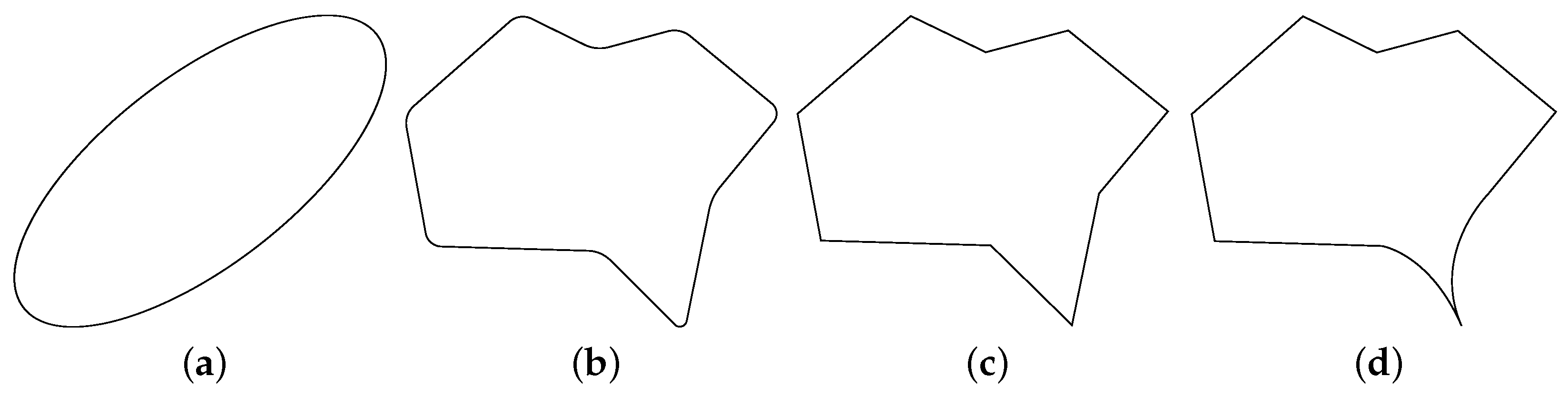
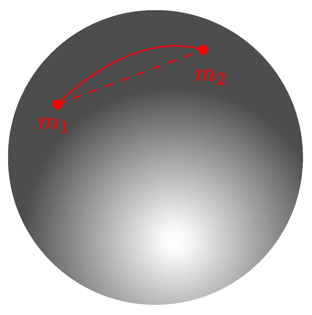
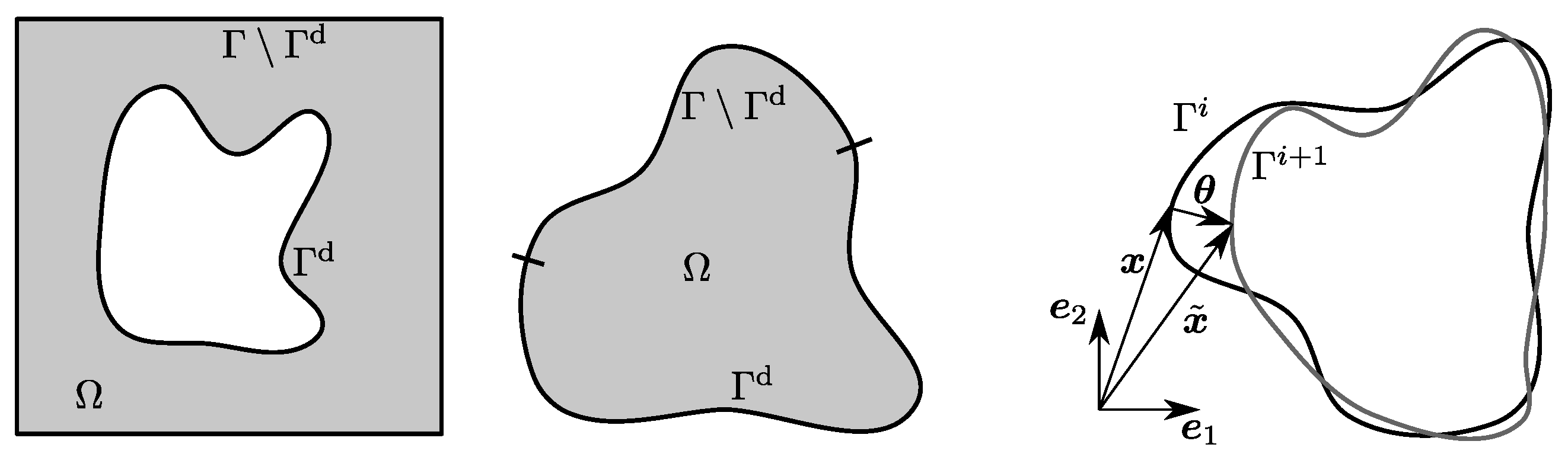
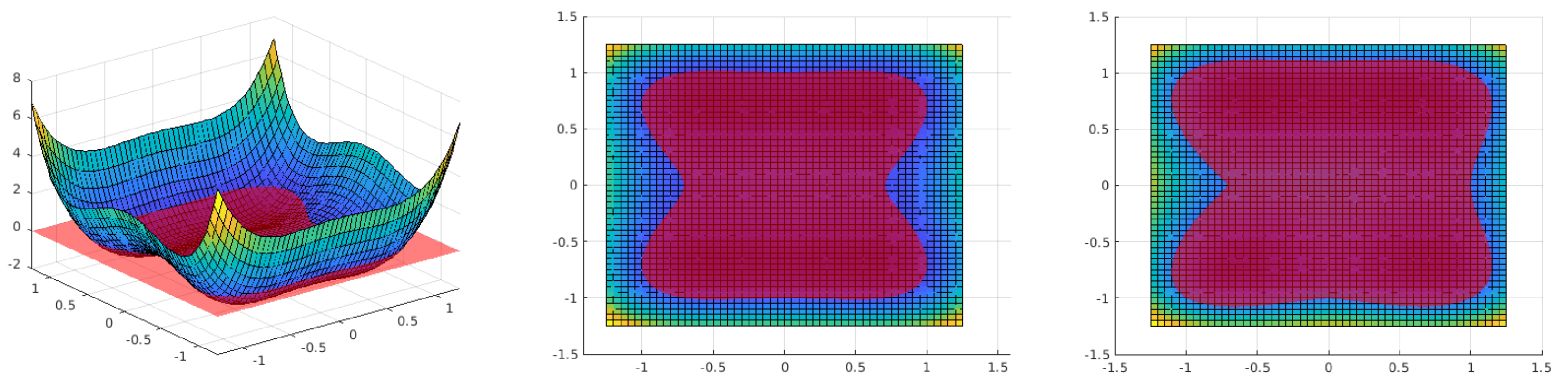
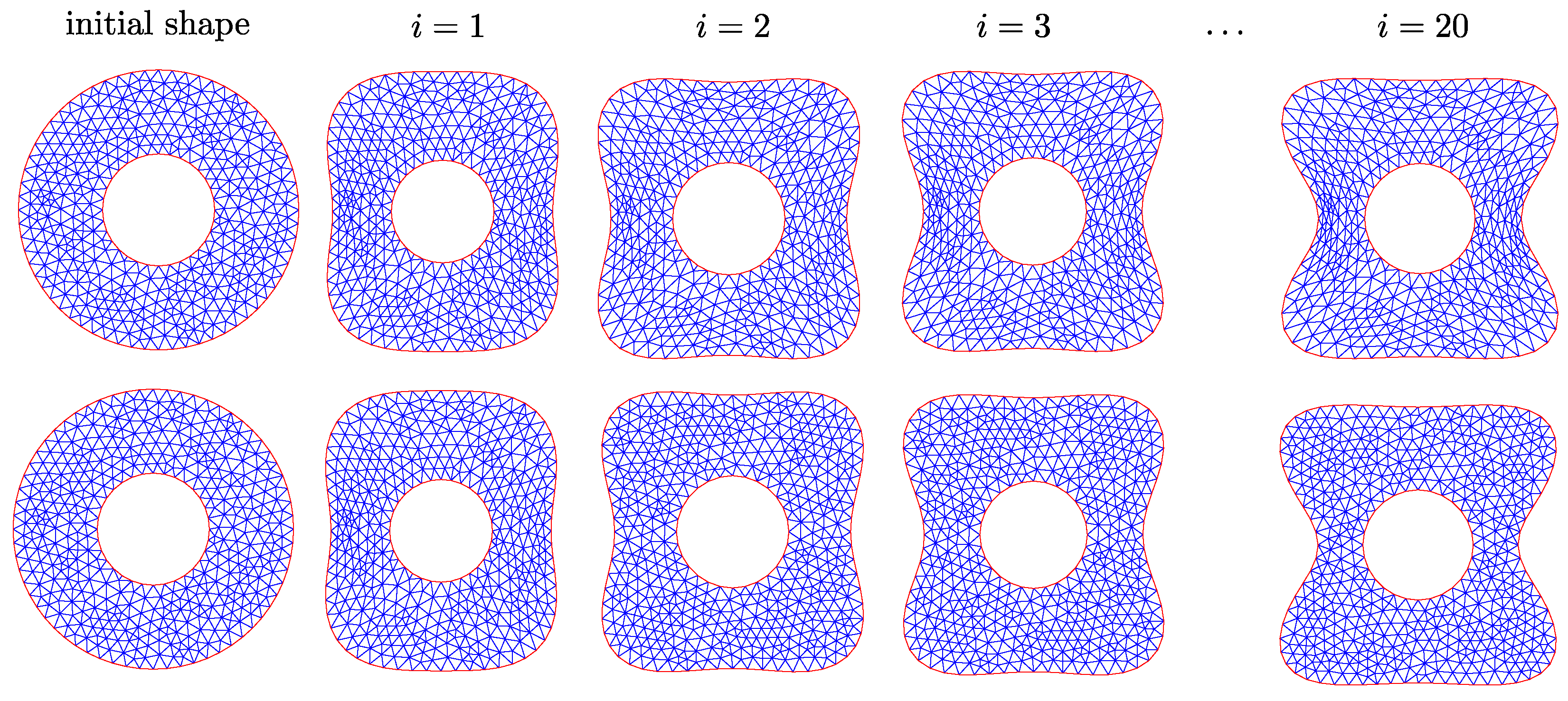
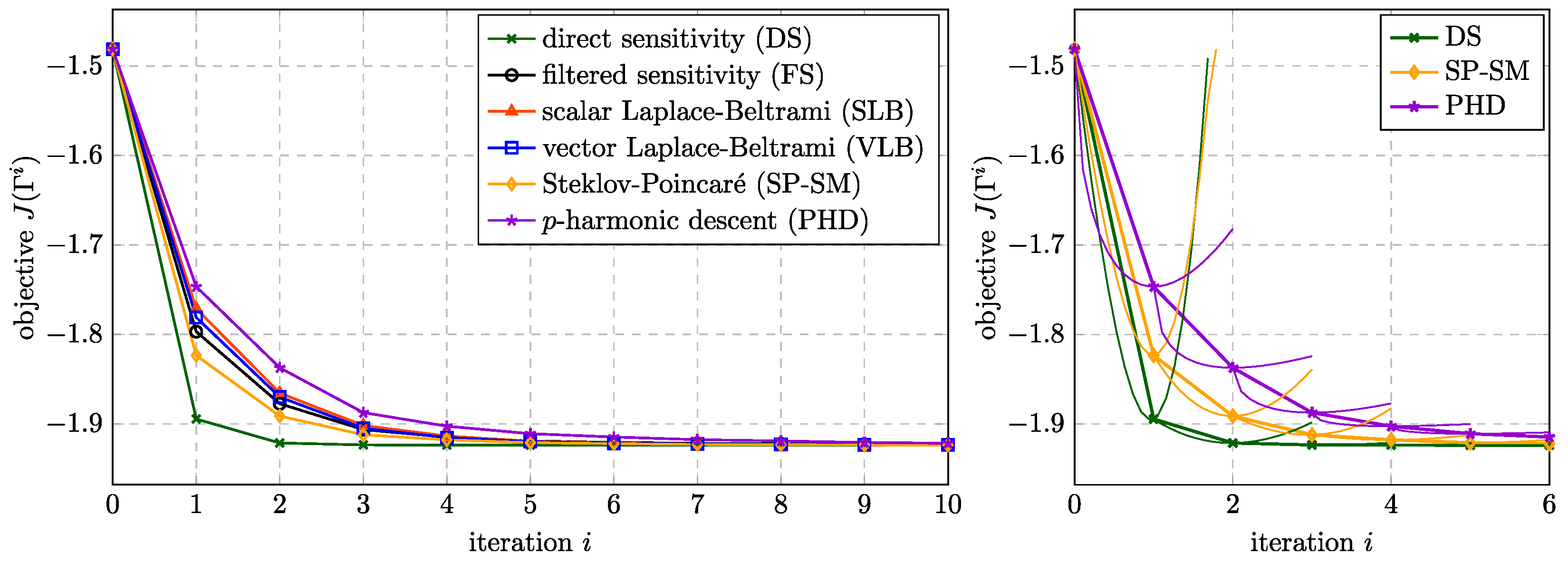
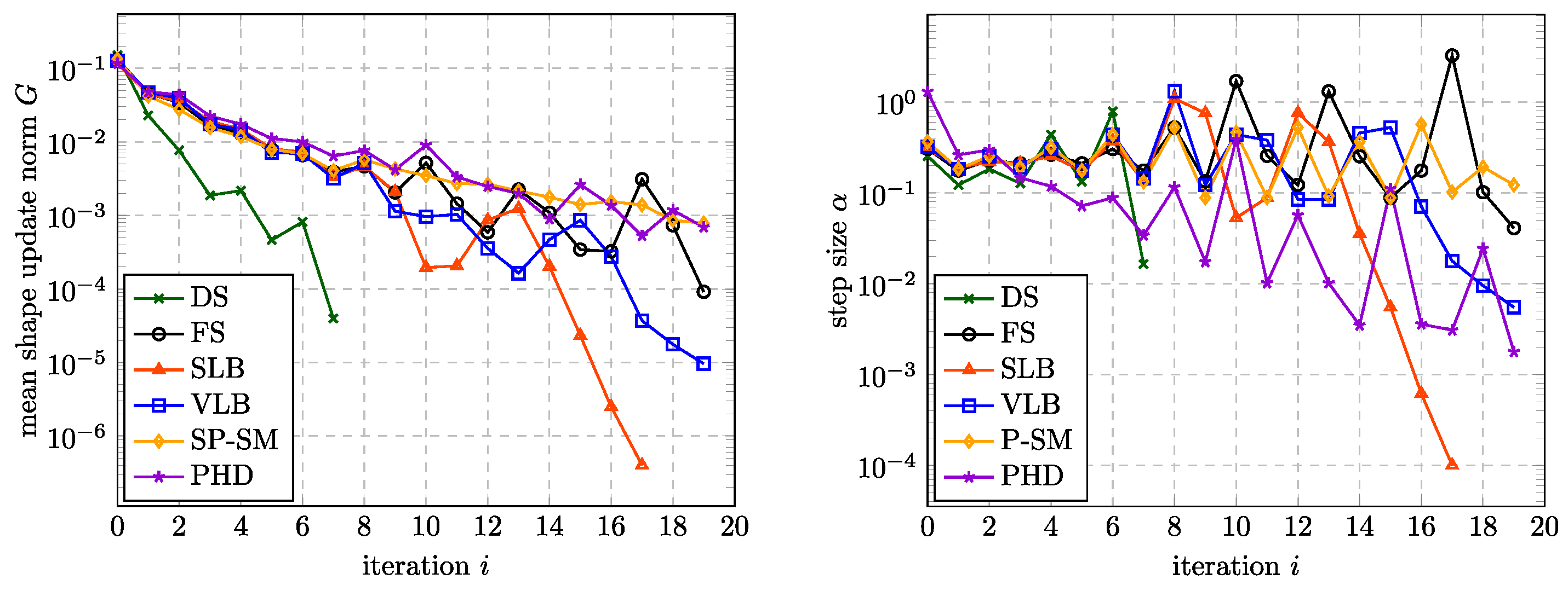
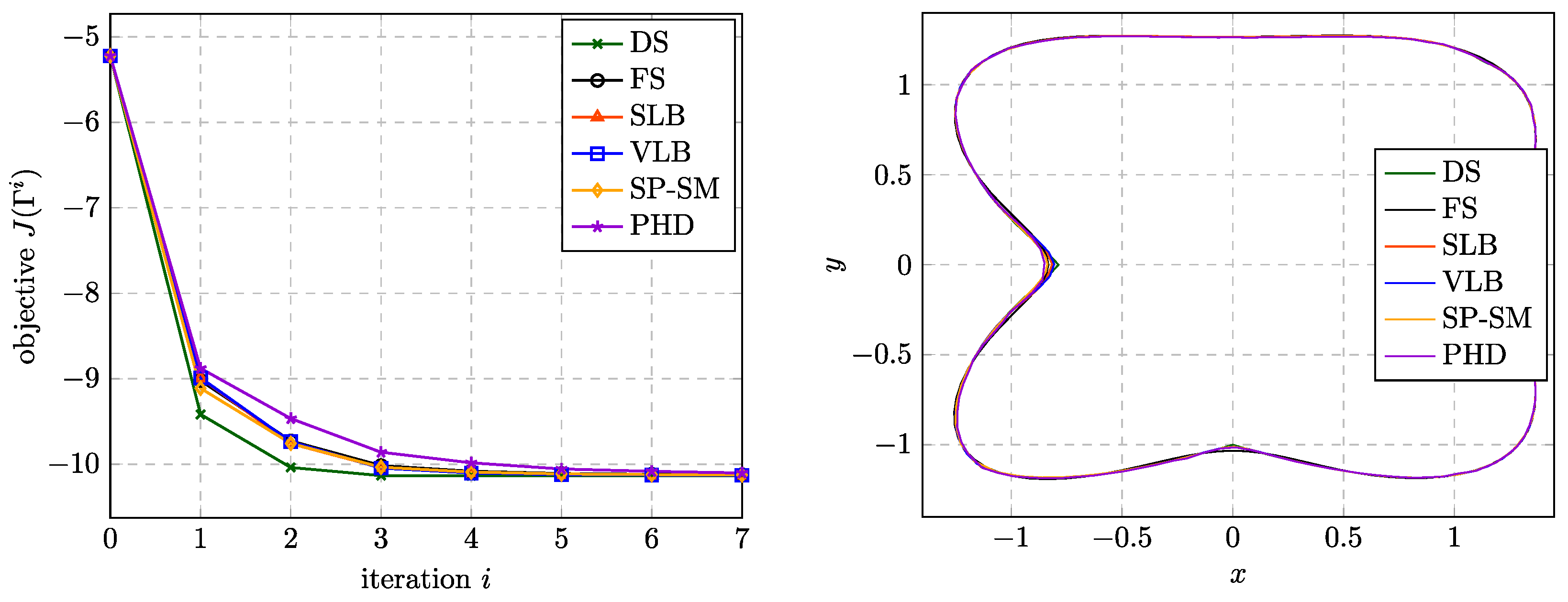
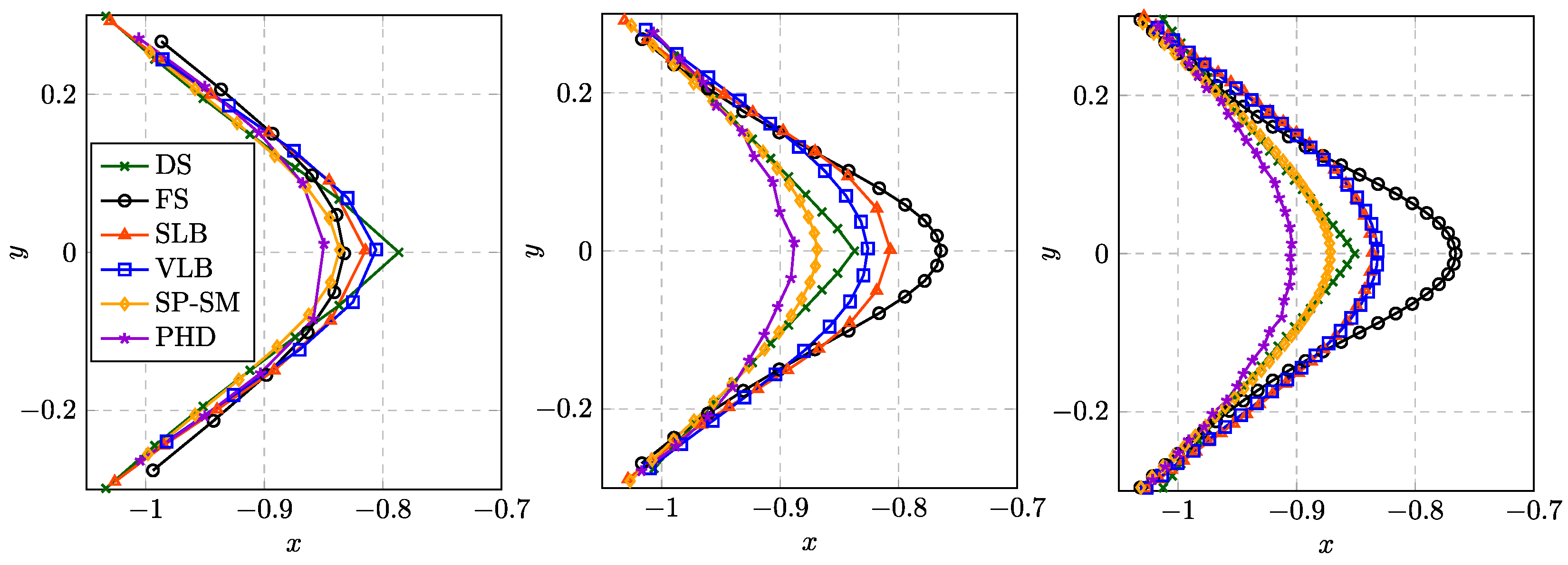
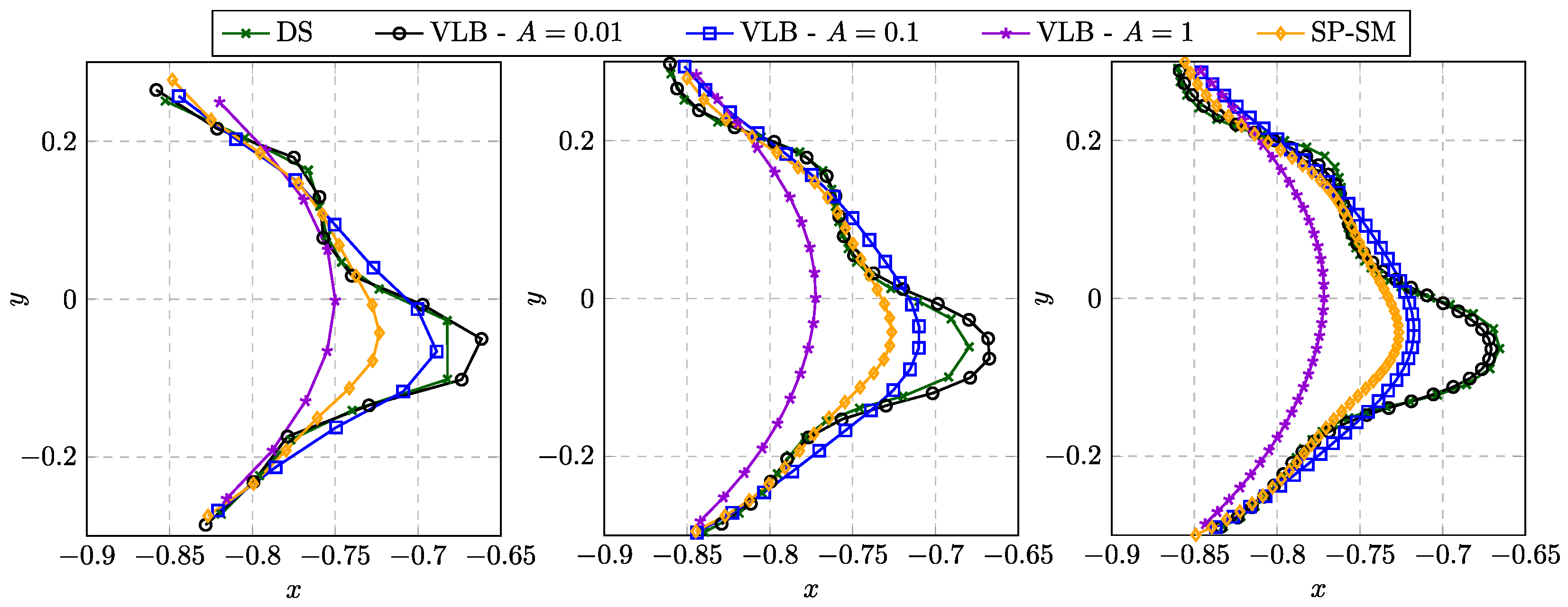
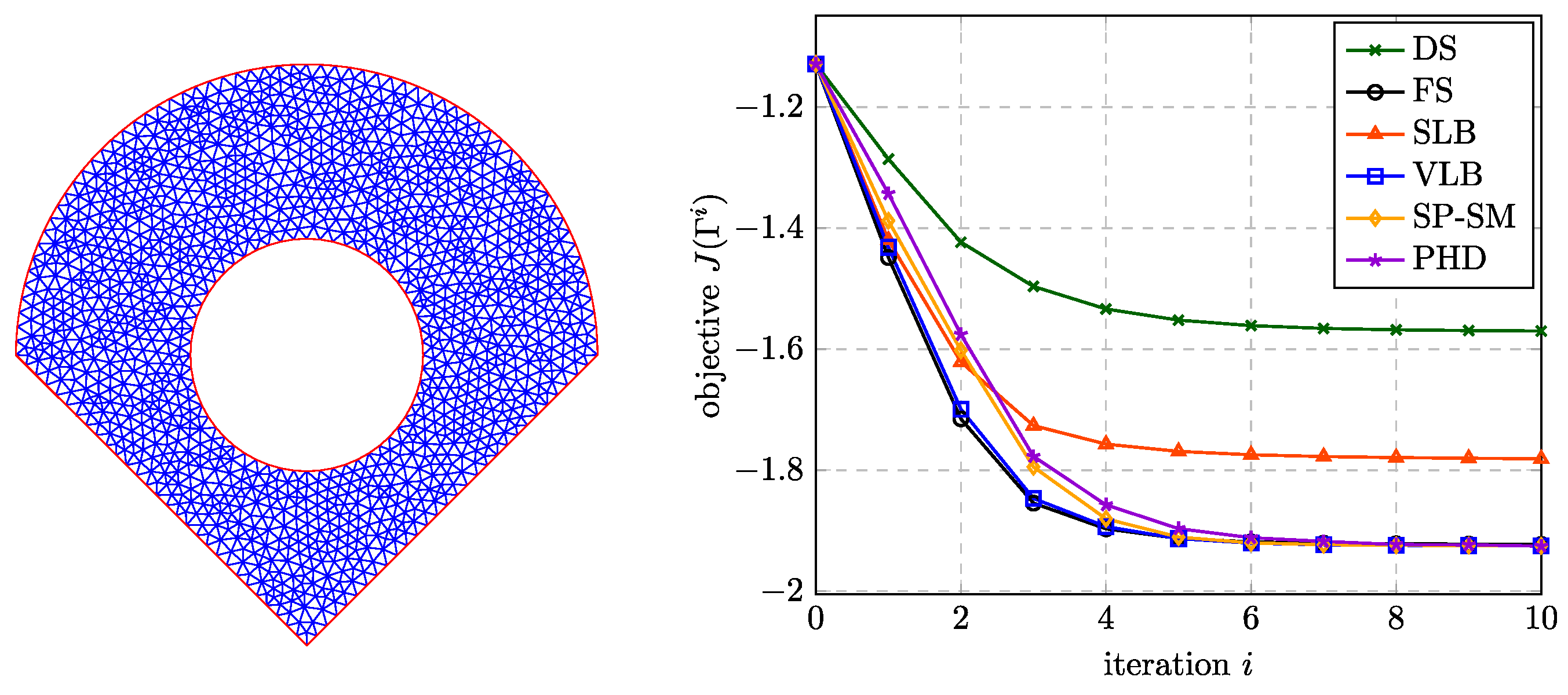
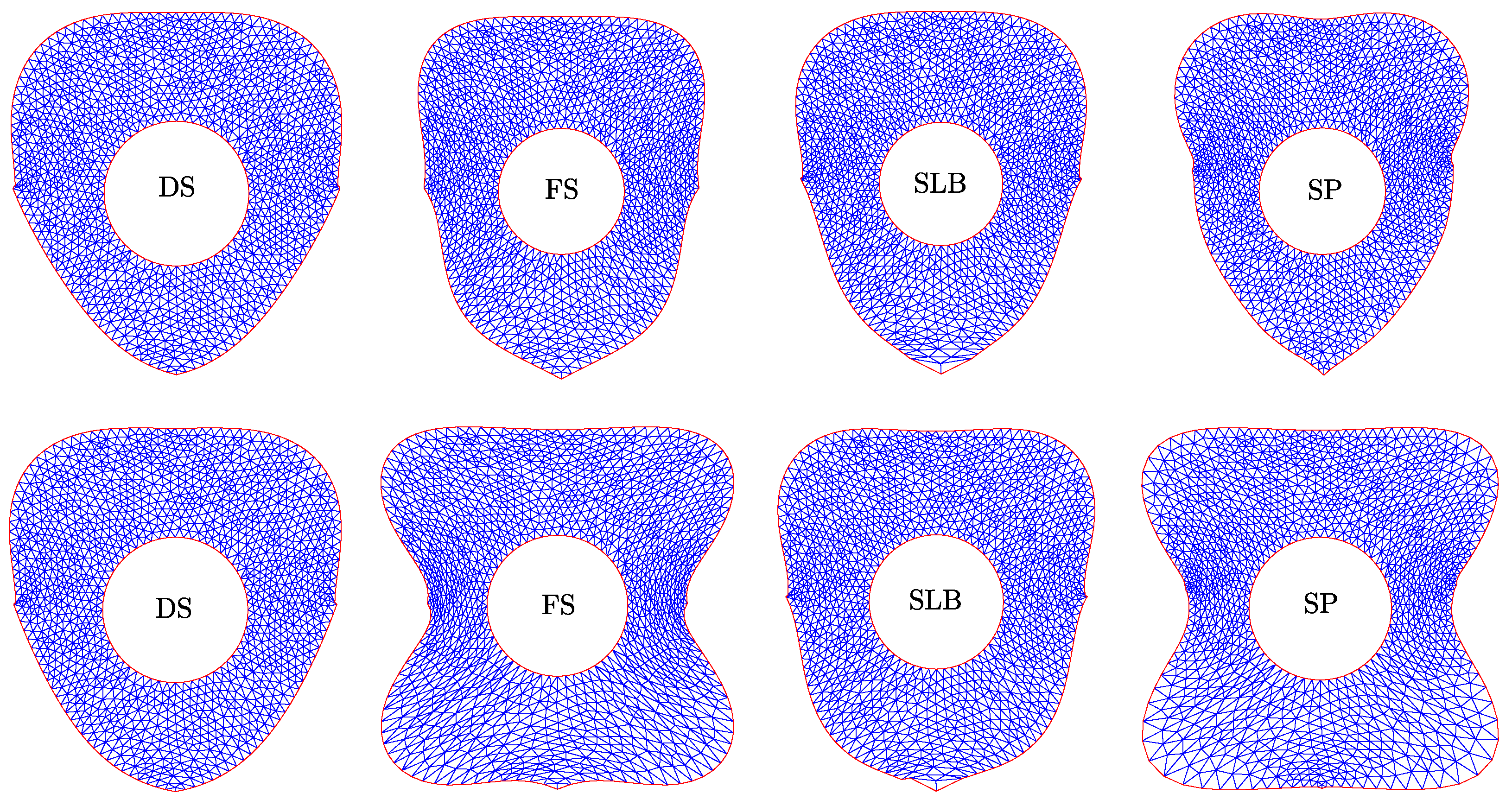
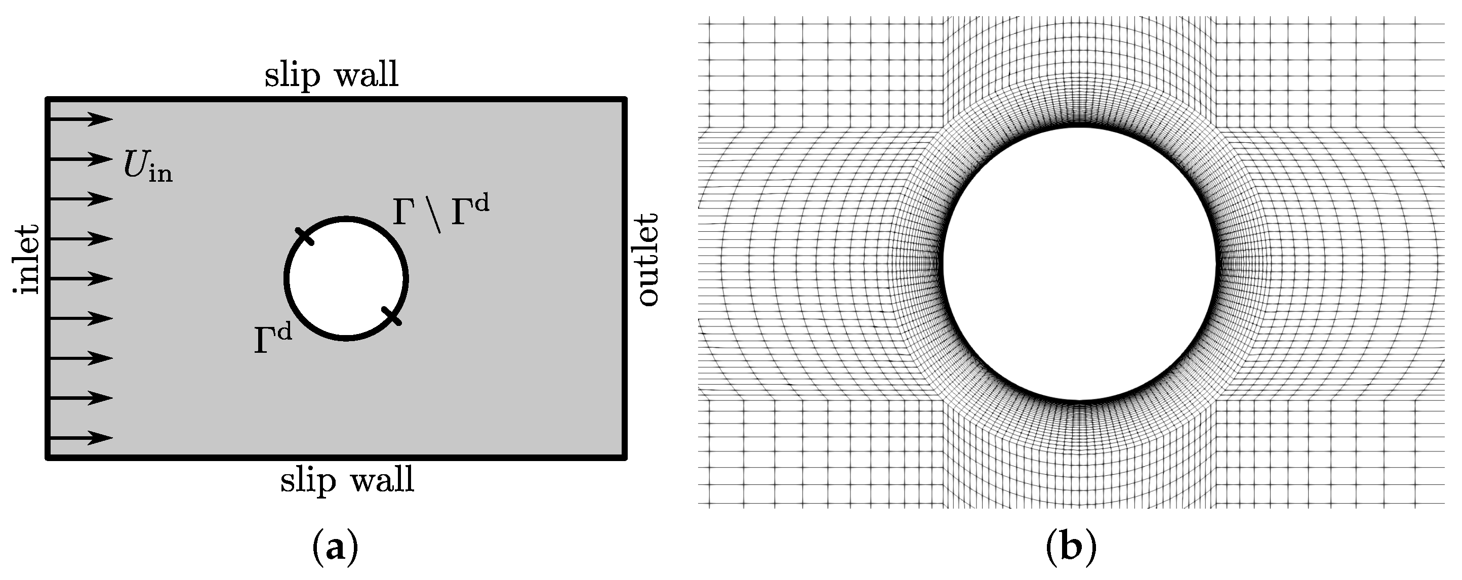
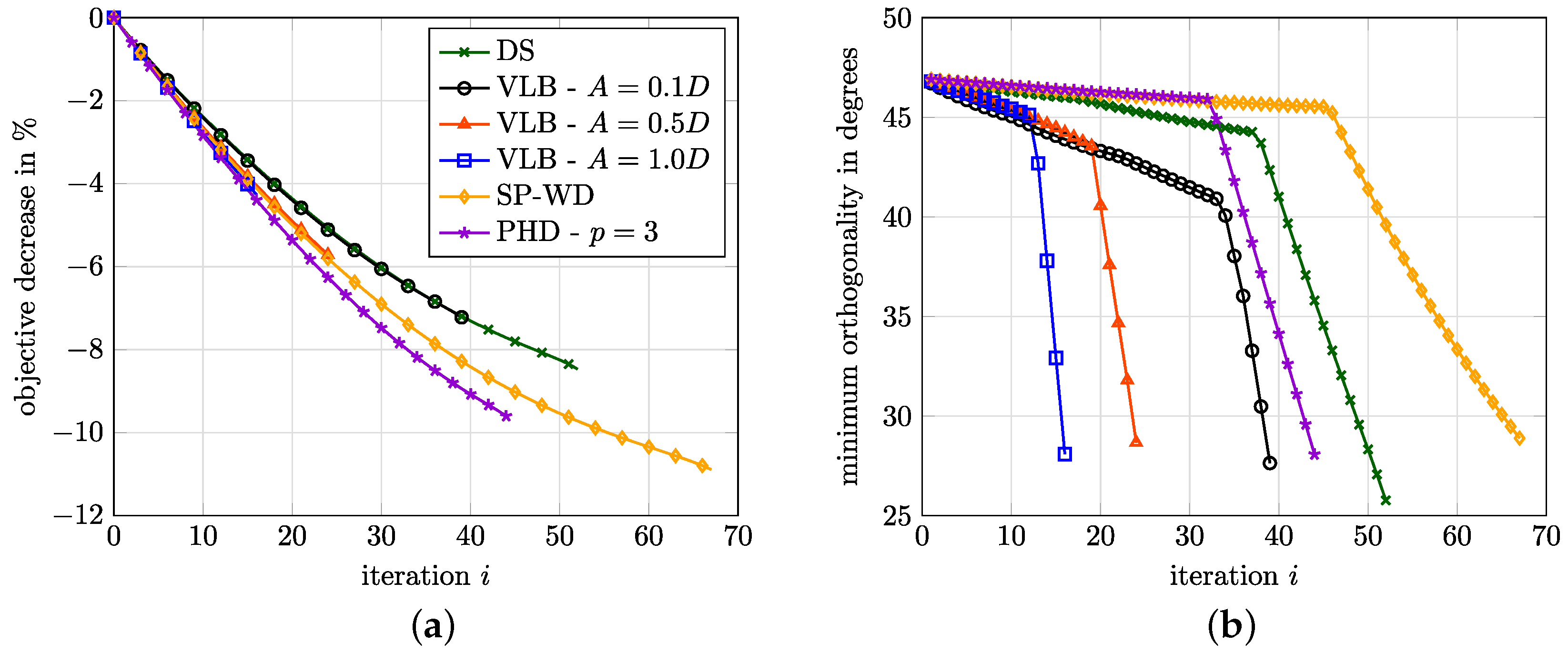
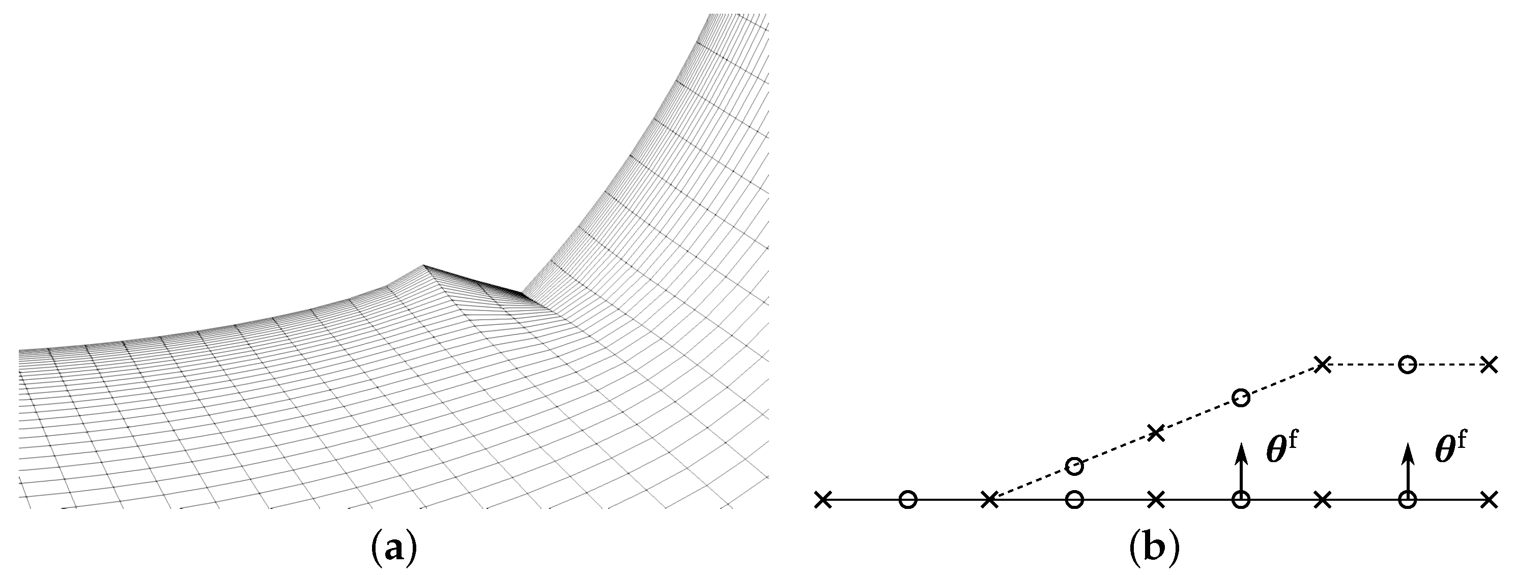
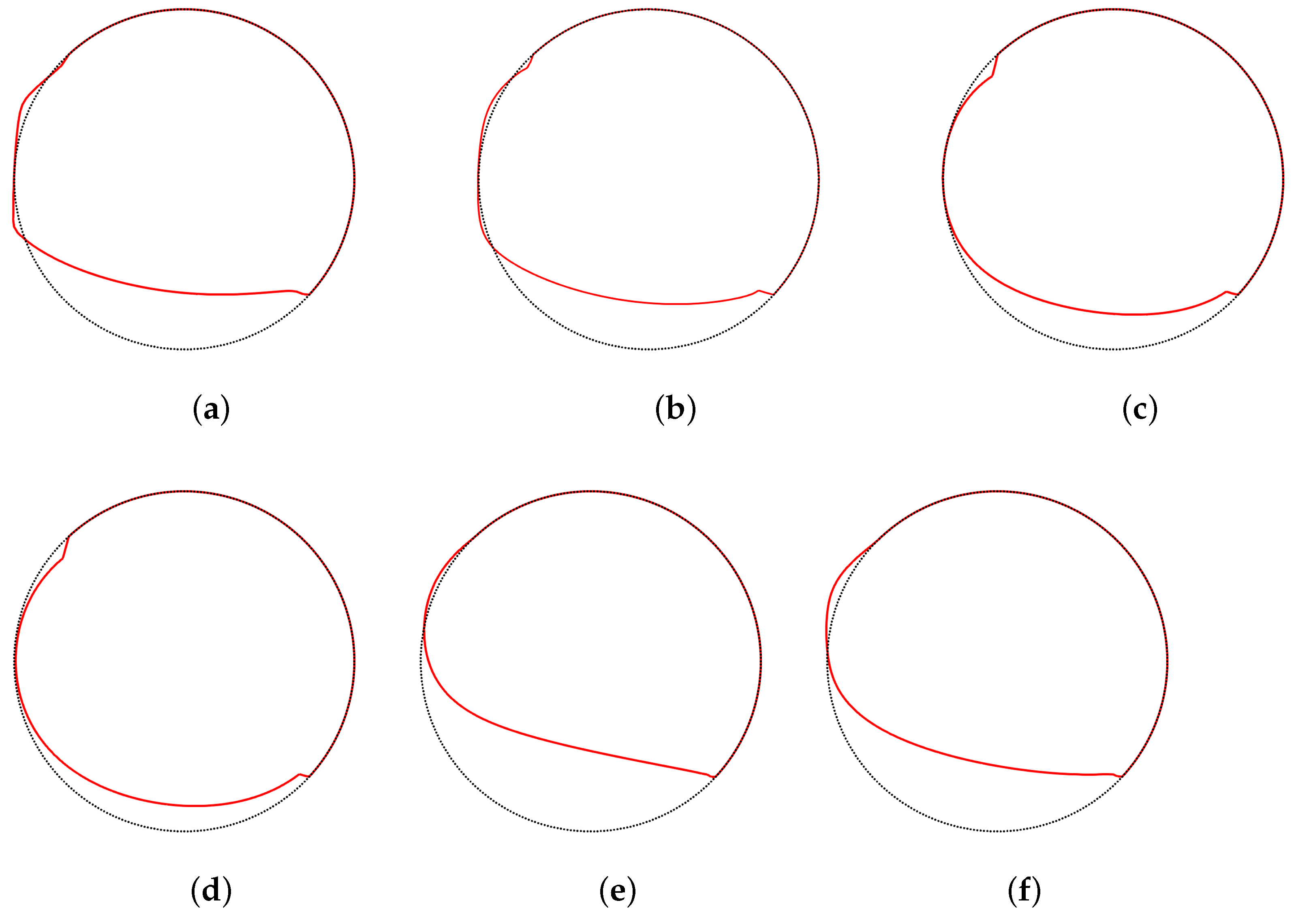
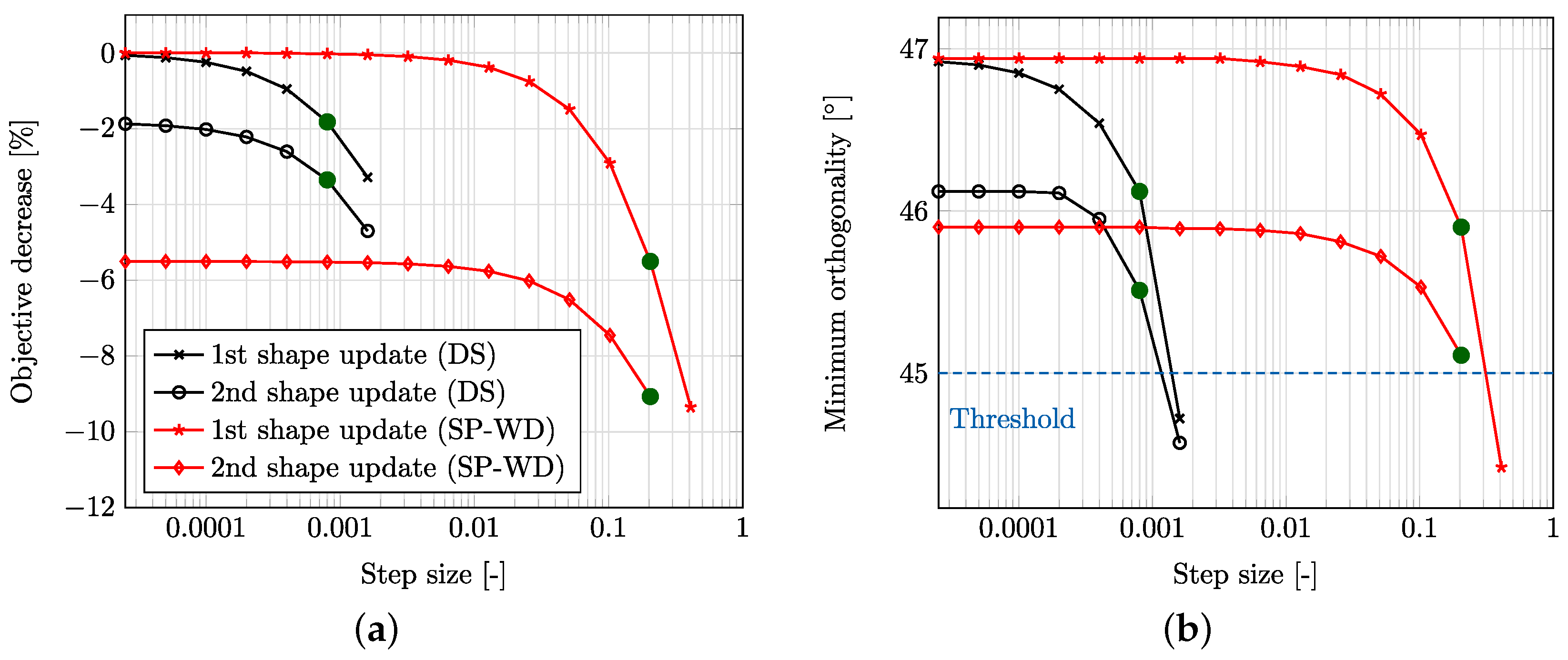
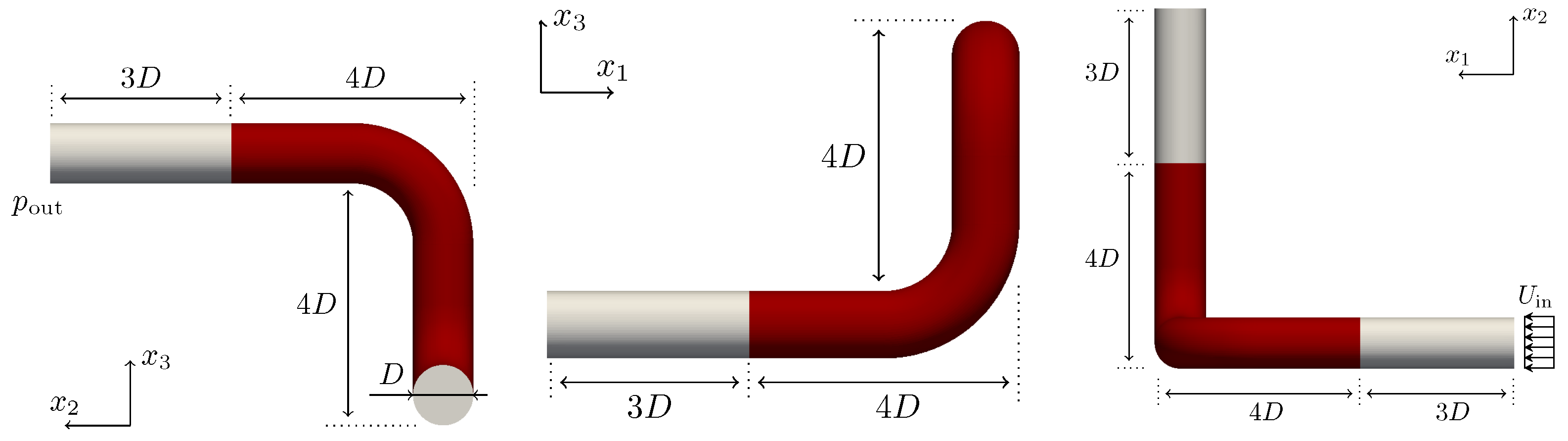
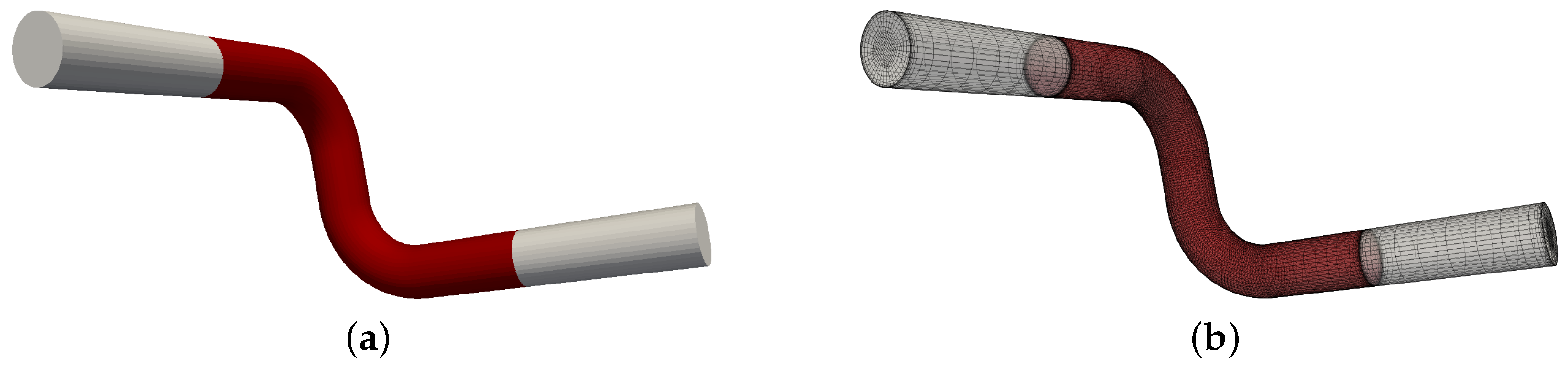
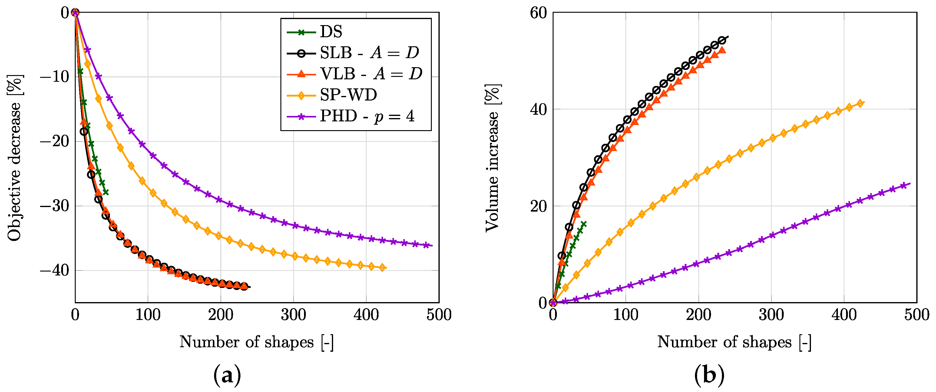
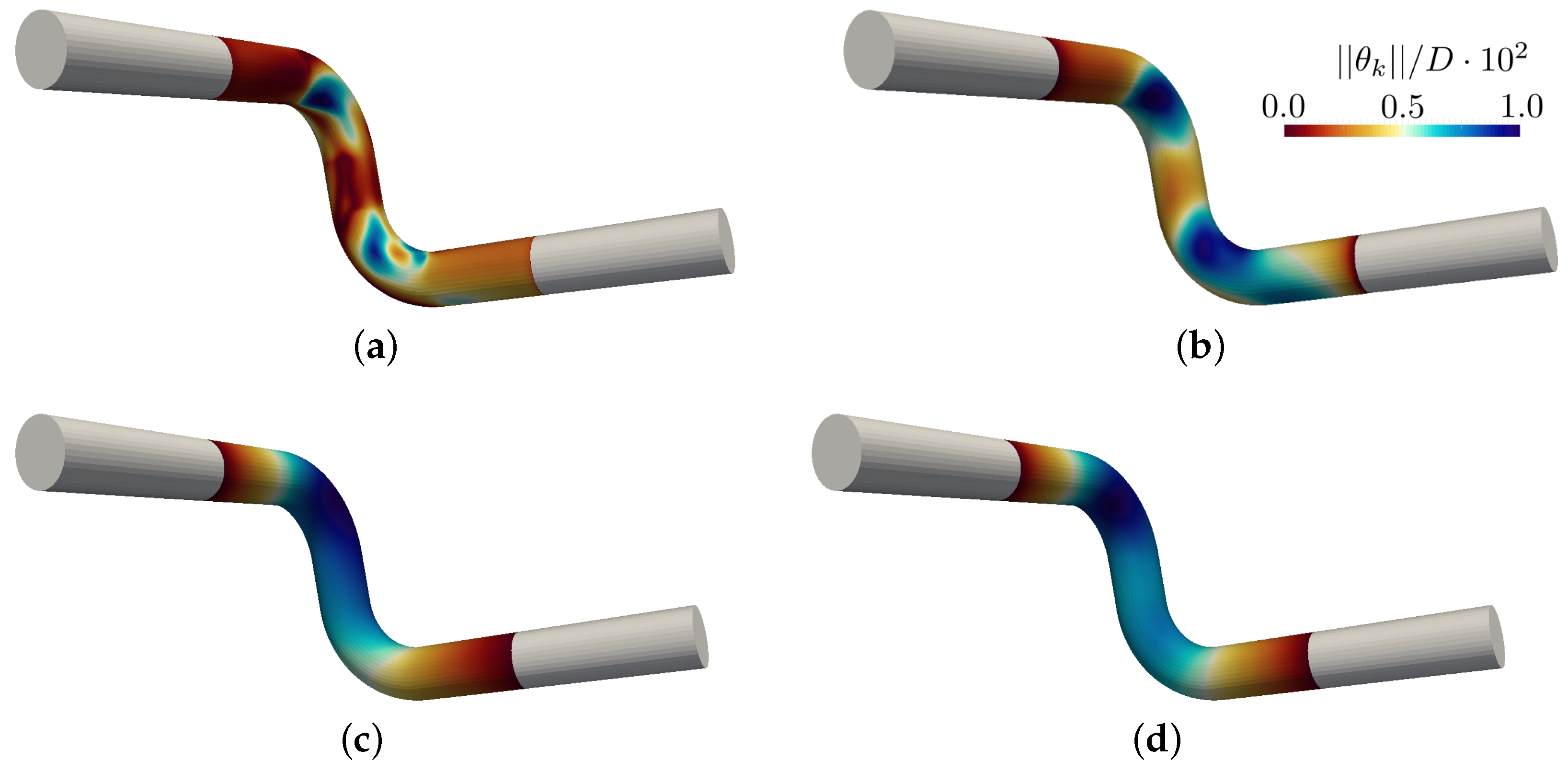
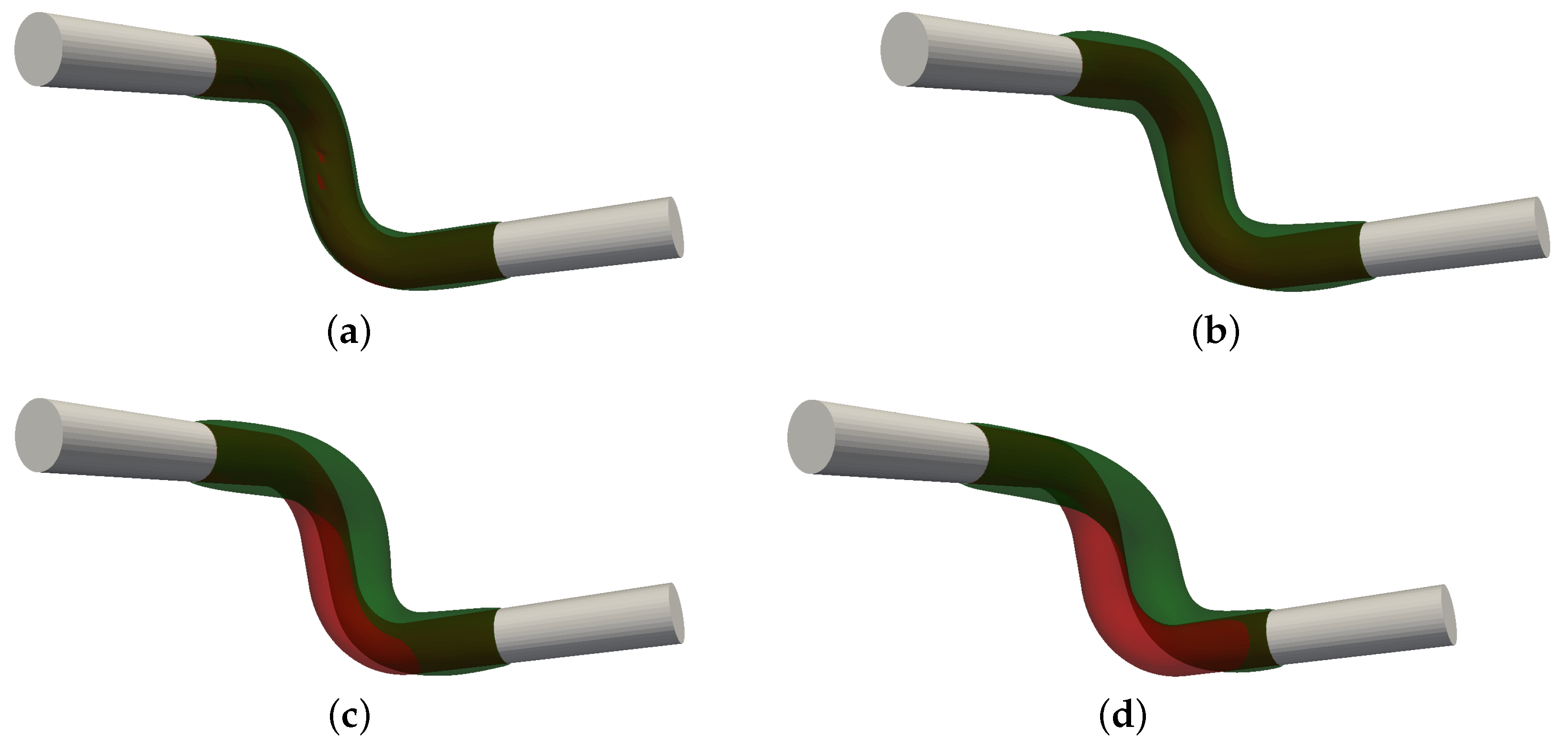
Table 1.
Overview of the approaches to compute a shape update.
| Approach | Abbreviation | Section | Auxiliary Problem |
|---|---|---|---|
| direct sensitivity | DS | Section 3.1.1 | |
| filtered sensitivity | FS | Section 3.1.1 | Equation (24) |
| vector Laplace–Beltrami | VLB | Section 3.1.2 | Equation (26) |
| scalar Laplace–Beltrami | SLB | Section 3.1.2 | Equations (29) and (30) |
| Steklov-Poincaré (struct. mechanics) | SP-SM | Section 3.1.3 | Equations (31) and (32) |
| Steklov-Poincaré (wall distance) | SP-WD | Section 3.1.3 | Equations (31) and (36) |
| p-harmonic descent | PHD | Section 3.1.4 | Equation (38) |
Table 2.
Cylinder (): Results of the mesh dependence study. For illustrative purposes, we denote here . Index i refers to the mesh refinement level. Note , , and .
Table 2.
Cylinder (): Results of the mesh dependence study. For illustrative purposes, we denote here . Index i refers to the mesh refinement level. Note , , and .
| Refinement Level | Number of FV | ||||
|---|---|---|---|---|---|
| M0 | 300 | 2.1197 | −3.325 | - | - |
| M1 | 1200 | 2.1433 | −3.612 | 1.11 | −8.64 |
| M2 | 4800 | 2.1356 | −3.822 | −0.35 | −5.81 |
| M3 | 19,200 | 2.1334 | −3.937 | −0.11 | −3.01 |
| M4 | 76,800 | 2.1334 | −3.932 | −0.003 | 0.14 |
| M5 | 307,200 | 2.1334 | −3.936 | −0.001 | −0.11 |
Table 3.
Double-bent pipe (): Results of the mesh dependence study. For illustrative purposes, we denote here . Index i refers to the mesh refinement level. Note , , and .
Table 3.
Double-bent pipe (): Results of the mesh dependence study. For illustrative purposes, we denote here . Index i refers to the mesh refinement level. Note , , and .
| Refinement Level | Number of FV | ||||
|---|---|---|---|---|---|
| M0 | 11,250 | 2.18 | −5.55 | - | - |
| M1 | 90,000 | 3.091 | −11.44 | 41.73 | 106.13 |
| M2 | 720,000 | 3.15 | −11.38 | 1.91 | −0.53 |
| M3 | 5,760,000 | 3.17 | −11.38 | 0.41 | 0.0 |
Table 4.
Double-bent pipe (): Measured computation time CPUh () for all five optimization studies, where refers to the mean wall clock time per primal/adjoint run and as well as denote the number performed optimization steps as well as employed CPU cores.
Table 4.
Double-bent pipe (): Measured computation time CPUh () for all five optimization studies, where refers to the mean wall clock time per primal/adjoint run and as well as denote the number performed optimization steps as well as employed CPU cores.
| Approach | [-] | Primal [h] | Adjoint [h] | Total CPUh [h] |
|---|---|---|---|---|
| DS | 42 | 0.1325 | 0.1176 | 10.5042 |
| SLB () | 241 | 0.1005 | 0.0994 | 48.1759 |
| VLB () | 235 | 0.0991 | 0.0981 | 46.342 |
| SP-WD | 441 | 0.1255 | 0.1109 | 86.9652 |
| PHD () | 491 | 0.1914 | 0.1070 | 146.5144 |
Disclaimer/Publisher’s Note: The statements, opinions and data contained in all publications are solely those of the individual author(s) and contributor(s) and not of MDPI and/or the editor(s). MDPI and/or the editor(s) disclaim responsibility for any injury to people or property resulting from any ideas, methods, instructions or products referred to in the content. |
© 2023 by the authors. Licensee MDPI, Basel, Switzerland. This article is an open access article distributed under the terms and conditions of the Creative Commons Attribution (CC BY) license (https://creativecommons.org/licenses/by/4.0/).
Share and Cite
MDPI and ACS Style
Radtke, L.; Bletsos, G.; Kühl, N.; Suchan, T.; Rung, T.; Düster, A.; Welker, K. Parameter-Free Shape Optimization: Various Shape Updates for Engineering Applications. Aerospace 2023, 10, 751. https://doi.org/10.3390/aerospace10090751
AMA Style
Radtke L, Bletsos G, Kühl N, Suchan T, Rung T, Düster A, Welker K. Parameter-Free Shape Optimization: Various Shape Updates for Engineering Applications. Aerospace. 2023; 10(9):751. https://doi.org/10.3390/aerospace10090751
Chicago/Turabian StyleRadtke, Lars, Georgios Bletsos, Niklas Kühl, Tim Suchan, Thomas Rung, Alexander Düster, and Kathrin Welker. 2023. "Parameter-Free Shape Optimization: Various Shape Updates for Engineering Applications" Aerospace 10, no. 9: 751. https://doi.org/10.3390/aerospace10090751
Note that from the first issue of 2016, this journal uses article numbers instead of page numbers. See further details here.