

Control of Cowl Shock/Boundary Layer Interaction in Supersonic Inlet Based on Dynamic Vortex Generator
by
 ,
,
Mengge Wang
1,2,
Ziyun Wang
1,*,
Yue Zhang
1,2,*,
Daishu Cheng
3,
Huijun Tan
1,
Kun Wang
1 and
Simin Gao
1 1
College of Energy and Power Engineering, Nanjing University of Aeronautics and Astronautics, Nanjing 210016, China
2
Laboratory of Aerodynamics in Muitiple Flow Regimes, China Aerodynamics Research and Development Center, Mianyang 621000, China
3
Zhengde Polytechnic, Nanjing 211106, China
*
Authors to whom correspondence should be addressed.
Aerospace 2023, 10(8), 729; https://doi.org/10.3390/aerospace10080729
Submission received: 6 July 2023
/
Revised: 31 July 2023
/
Accepted: 15 August 2023
/
Published: 20 August 2023
(This article belongs to the Special Issue Shock-Dominated Flow)
Abstract
:A shock wave/boundary layer interaction (SWBLI) is a common phenomenon in supersonic inlet flow, which can significantly degrade the aerodynamic performance of the inlet by inducing boundary layer separation. To address this issue, in this paper, we propose the use of a dynamic vortex generator to control the SWBLI in a typical supersonic inlet. The unsteady simulation method based on dynamic grid technology was employed to verify the effectiveness of the proposed method of control and investigate its mechanism. The results showed that, in a duct of finite width at the inlet, the SWBLI generated complex three-dimensional (3D) flow structures with remarkable swirling properties. At the same time, vortex pairs were generated close to the side wall as a result of its presence, and this led to the intensification of transverse flow and, in turn, the formation of a complex 3D structure of the flow of the separation bubble. The dynamic vortex generator induced oscillations of variable intensity in the vortex system in the supersonic boundary layer that enhanced the mixing between the boundary layer flow and the mainstream. Meanwhile, the unique effects of “extrusion” and “suction” in the oscillation process continued to charge the airflow, and the distribution of velocity in the boundary layer significantly improved. As the oscillation frequency of the vortex generator increased, its charging effect on low-velocity flow in the boundary layer increased, and its control effect on the flow field of the SWBLI became more pronounced. The proposed method of control reduced the length of the separation bubble by 31.76% and increased the total pressure recovery coefficient at the inlet by 6.4% compared to the values in the absence of control.
1. Introduction
As an essential part of aspirated high-speed propulsion systems, the inlet has many functions, such as capturing flow, converting the energy of the incoming flow, regulating the velocity of flow at the outlet, and isolating the upstream and downstream disturbances. These functions profoundly influence the efficiency and working envelope of the engine [1]. The capture and deceleration of airflow in supersonic/hypersonic inlets primarily rely on the generation of shock waves and compression-induced wave systems. However, the inlet inevitably produces a boundary layer during its operation and may also ingest it from the forebody under conditions of integration to give rise to a shock wave/boundary layer interaction (SWBLI). This phenomenon is inherent to supersonic/hypersonic inlets and significantly impacts their performance. Specifically, the SWBLI at the entrance of the inlet is often intense at higher Mach numbers and may cause significant boundary layer separation. This is because the local adverse pressure gradient of the boundary layer introduced by the cowl shock exceeds its limit of separation and leads to apparent separation within the inlet, causing a compression–expansion–recompression flow process. SWBLIs, in general, lead to boundary layer separation, which causes a large decrease in total pressure, large distortion at the face of the engine, and potentially results in an inlet unstart [2]. In order to ensure the safe and efficient operation of an inlet within the entire envelope of operation of the engine, the complex phenomenon of the SWBLI in the inlet must be controlled [3,4].
Various methods of flow control have been proposed by researchers worldwide. Active methods of flow control primarily include boundary layer bleeding and blowing. The bleeding method removes low-energy fluid from the boundary layer before separation [5] and can suppress boundary layer separation. Blowing involves injecting high-pressure flow into the boundary layer to improve its ability to resist the adverse pressure gradients induced by the SWBLI [6]. However, both methods have drawbacks. Bleeding requires the removal of a portion of the flow captured by the inlet and complex suction structures, which incurs additional bleeding-induced resistance. Moreover, while blowing can weaken the effect of the SWBLI in a specific range, it requires a high-pressure source, which makes it less feasible.
Passive methods of flow control, such as vortex generators (VG) [5,6,7,8], have become a focus of research on controlling SWBLIs due to their simple construction, ease of installation, and greater degree of control. VGs introduce counter-rotating vortices to the flow without additional energy. These vortices transfer high-momentum flow to the wall, and this results in a fuller boundary layer profile. However, the additional shape-induced drag caused by traditional VGs creates strong disturbances in the mainstream that affect the overall efficiency of the aircraft. Consequently, researchers have shifted their focus to micro-vortex generators (MVG) [9], as they can significantly reduce the additional drag due to the components of control. MVGs have a height that is only 10–60% of the thickness of the boundary layer and can still achieve the desired control effects [9,10]. Significant progress has been made in the development of MVGs in recent years [11,12]. Blinde et al. [13] conducted detailed studies on the flow field in the SWBLI under MVG-based control. The results showed that the presence of the MVG reduced the region of separation from 20% to 30%, and the amplitude of the incident shock-induced oscillations was reduced by 20% compared with the condition without MVG-based control. Anderson et al. [14] demonstrated that triangular wedge- and blade-shaped MVG arrays can generate counter-rotating vortices and create alternating spatial distributions of the upwash and downwash in the spanwise direction that intensify the exchange of energy between the inner and outer fluids of the boundary layer to make it fuller. Zhang [15] proposed and assessed a highly swept ramp-type MVG that induced a “precompression effect,” a “dividing effect,” and a “mixing effect” due to the unique structure of the vortex generator. This phenomenon suppressed boundary layer separation and promoted the reattachment of the separated flow.
Moreover, researchers have explored combined methods of flow control. Anderson et al. [16] improved an active control system for an S-shaped inlet by adding an MVG to the rear of the jet to achieve the same control effect as that when the jet flow was reduced to one-tenth of its original rate of flow. Wagner et al. [17] found that placing an MVG at the inlet led to a 32% increase in maximum back-pressure and a 34% improvement in pressure stability within the isolation region when the inlet was in a stable start-up state.
In this paper, we propose a dynamic vortex generator (hereinafter referred to as the “dynamic MVG”) for controlling the cowl-induced SWBLI in a typical supersonic inlet. The dynamic MVG can not only generate wake-induced vortices but also inject energy upstream of the SWBLI. Its influence on the SWBLI was studied using unsteady numerical simulations combined with the dynamic grid technique. The mechanism of control and effects of the MVG on supersonic inlets are also discussed in this paper.
2. Concept of Dynamic MVG Control
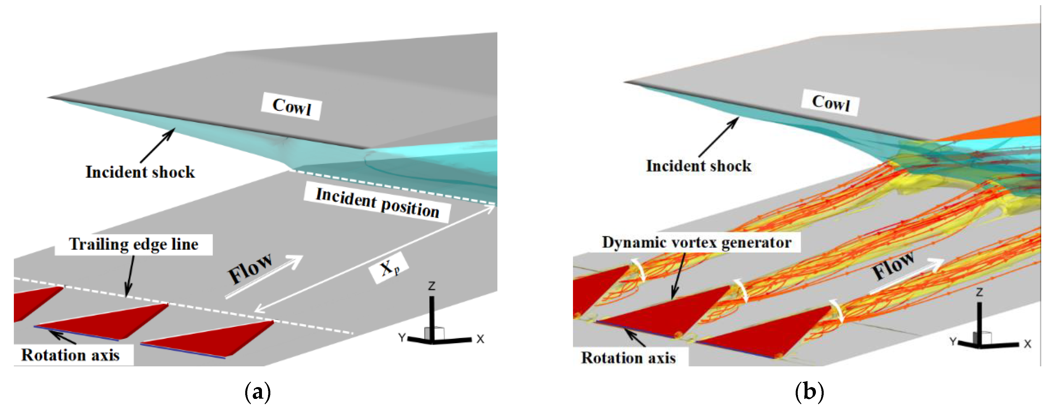
In order to enhance the ability of the supersonic inlet boundary layer to resist the adverse pressure gradient, a SWBLI control method based on an array of dynamic MVGs is proposed in this paper. Figure 1 shows that the array configuration of the vortex generators was obtained by lining them up along the spanwise direction. The array was composed of three dynamic MVGs to improve their range of control. This is also the minimum number of units that can accurately reflect the characteristics of interaction between the vortices generated by them. Its specific mode of operation is as follows: The vortex generator is placed at position Xp upstream of the point of incidence of the shock (Xp is the distance between the trailing edge of the vortex generator and the point of incidence of the shock). When the SWBLI does not cause significant boundary layer separation, the flow does not need to be controlled. The vortex generator is embedded into the wall of the inlet to keep it flat and avoid increasing the resistance in the duct. When large-scale boundary layer separation is induced by the SWBLI at the inlet, the dynamic MVG oscillates around its axis of rotation at high frequencies to induce dynamic vortices of higher intensity that yield stronger momentum mixing and lead to an increase in the suppression of the separation.
3. Methodology
3.1. Description of the Model
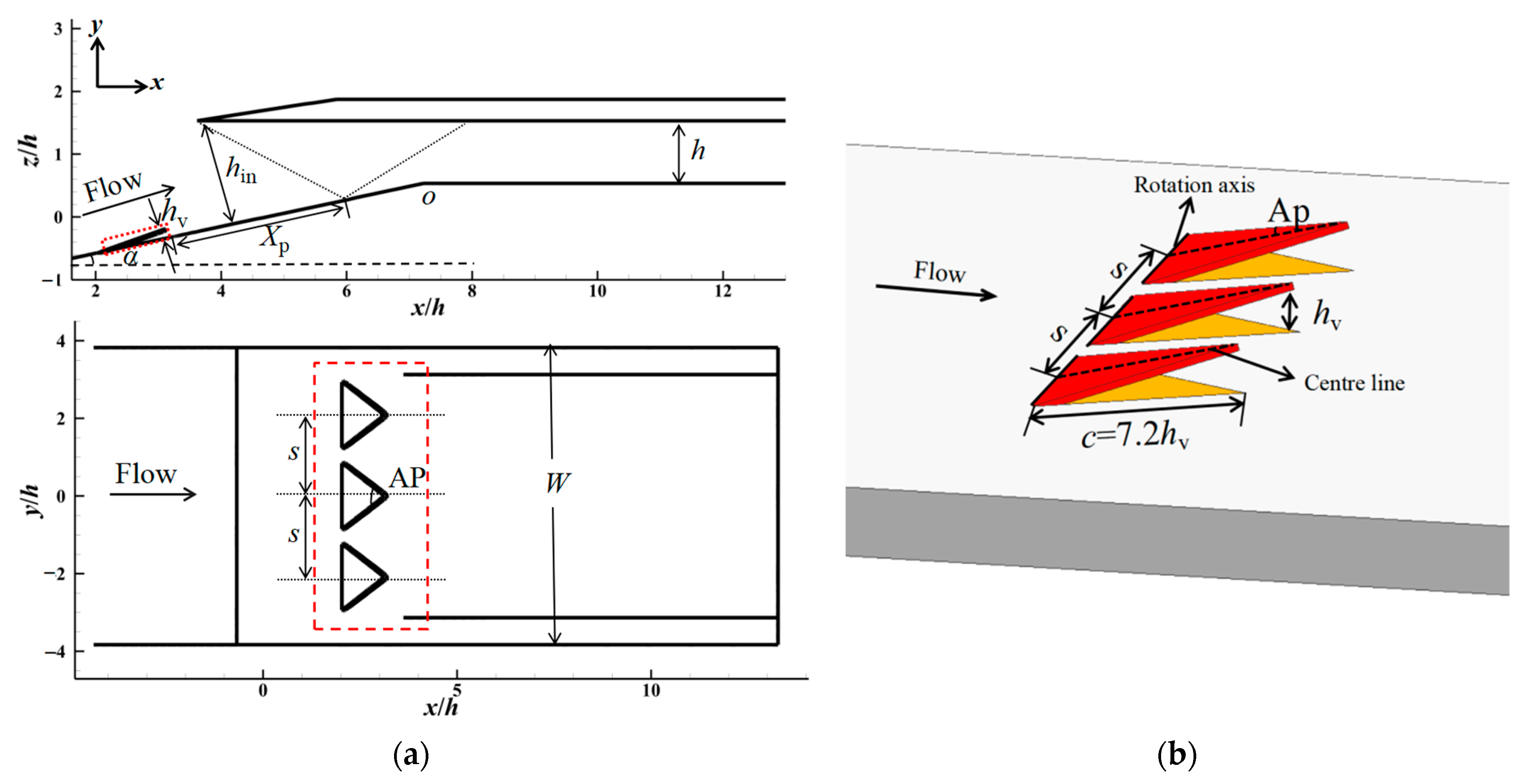
The dynamic MVG was placed in a supersonic inlet with a working Mach number of 3.8 to verify its capability of control. Figure 2 shows the two-dimensional (2D) schematic diagram of the inlet. Its angle of compression α in the first stage was 12°, the height of the entrance to the duct (hin) was 24.9 mm, and its height h was 14.4 mm. The red dotted box is used to highlight the vortex generator location. According to the design principle of the proposed dynamic MVG, the array of dynamic MVGs was arranged upstream of the shoulder of the inlet O to ensure that the point of incidence of shock was at a certain distance from the trailing edge of the vortex generator. According to the reference value of the position of shock incidence in [18,19], for this paper, we selected 10hv as the distance Xp between the trailing edge of the dynamic MVG and the point of shock incidence. The basic configuration of the dynamic MVG proposed in this study was designed using the methods in [14,18], and its configuration is also the basic configuration commonly used by other researchers, and it can ensure the optimal control effect of the vortex generator [11,13,20]. The maximum height of oscillations of the dynamic MVG was hv, an order of the thickness of the incoming boundary layer ẟ, and the spacing between the centerlines of two MVGs was s = 7.5hv. The half-top angle AP of the dynamic MVG was 24°, and the chord length c was 7.2 times the dynamic MVG height hv. The typical geometric parameters are listed in Table 1. Note that the dynamic MVG was a thin plate-type generator with a thickness d of 0.5 mm; the leading edge was chamfered, and there was a 0.1 mm margin between the perimeter of the vortex generator and the bottom wall. The MVG (three in a group) oscillated periodically around the axis of oscillation of the leading edge of the vortex generator at a frequency of 100 Hz.
This paper establishes a coordinate system, with the x-axis direction representing the flow direction, the y-axis direction representing the extension of the flow field, and the z-axis direction representing the perpendicular wall normal. Figure 3 shows the variations in the flow field of the array of vortex generators along the directions of flow (x–z plane) and the extension (y–z plane); the flow characters on different flow direction positions and extension directions are discussed in this paper. The distribution of pressure and velocity on these cross sections were analyzed; x was defined as the distance between the measurement position and the trailing edge of the vortex generator, and y represented the distance to the vortex generator symmetric plane y = 0hv. The static pressure and temperature of the incoming flow were given according to atmospheric conditions at a flight altitude of 20 km. For a freestream Mach number Ma0 of 3.8, the freestream flow pressure p0 is 5529 Pa, and the static temperature T0 is 216 K; therefore, the total pressure P* is 640 kPa, and the total temperature T* is 842 K. Due to the forebody compression surface, an oblique shock wave is generated at the front edge of the compression surface, resulting in a deceleration of airflow after passing through this shock wave. As a result, upstream of the vortex generator, there is a decrease in Mach number to 3.0. The velocity u and wall-normal direction distance z are dimensionless treated with freestream streamwise velocity u0 and vortex generator height hv, respectively, and the static pressure p is dimensionless treated with the freestream flow pressure p0.
3.2. Numerical Approach
3.2.1. Numerical Method
The dynamic mesh method in ANSYS FLUENT can be used to model flows where the shape of the domain changes with time due to motion in the domain boundaries. The MVGs were dynamically adjusted through unsteady numerical simulations, and spring smoothing and local reconstruction were used in the algorithm for the dynamic mesh. The update of the volume mesh is handled automatically at each time step based on the new positions of the boundaries. To use the dynamic mesh model, it is necessary to provide a starting volume mesh and a description of the motion of any moving zones in the model. The motion of these zones can be defined using a user-defined function (UDF) in ANSYS FLUENT, and the moving part was set to the motion of a rigid body rotating about a fixed point. Because the model contains moving and non-moving regions, it is important to identify these regions by grouping them into their respective cell zones in the starting volume mesh. Furthermore, regions deforming as a result of motion on their adjacent regions must also be grouped into separate zones in the starting volume mesh.
The grid topology of the model of the inlet and the array of dynamic MVGs are shown in Figure 4. The interface divided the entire computational domain into a non-moving domain (on the left) and a moving inner domain (on the right). Mixed grids were used for the calculations to satisfy the requirements of the method to update the dynamic grid. Unstructured grids were used near the vortex generator (right figure) to ensure that the grid could be updated and reconstructed during the motion of the vortex generator, while structural grids were used in the other areas (left figure) to ensure the quality of the grid. Maintain consistent surface mesh distribution at the interface between structured and unstructured grids, and set the boundary condition to the interface.
The total number of grid nodes was about 15.9 million, and the y+ of the near-wall grid was guaranteed to be less than 1. In addition, the grid downstream of the vortex generator was encrypted to capture the structure of the flow of the vortex generator. The boundary conditions of the flow field were set as follows: The bottom and side walls were set to adiabatic solid-wall boundaries. The left and right sides were set as the side walls (hidden in order to better show the internal grid); the boundaries of pressure at the outlet were imposed on all outlets, and the other surfaces were subjected to the far-field boundary conditions of pressure.
To balance the efficiency of the search for appropriate values of the parameters with the accuracy of the calculations, calculations based on the 3D unsteady Reynolds-averaged Navier–Stokes (URANS) equations were carried out using the Computational Fluid Dynamics (CFD) software ANSYS FLUENT. This was carried out as follows: The inviscid convection flux is discretized by Roe’s approximated Riemann method [21], and the interface flux is interpolated using Monotone Upwind Scheme for Conservation Laws (MUSCL) to obtain the second-order difference scheme of the inviscid convection flux. At the same time, the viscous flux is discretized through the second-order upwind scheme. The ideal gas model was used for the calculations, and the Shear Stress Transport (SST) k-ω model was used to model the turbulence [22]. In a previous study in the literature, a RANS solver, based on the SST turbulence model in FLUENT, was successfully applied to the flow with SWBLI, and the results of this study are in good agreement with experimental results [23,24,25,26]. The viscosity coefficient follows the Sutherland formula [27]. Moreover, the Mach number at the exit of the duct and mass flow through the exit were monitored in the simulations, and it was ensured that the residual convergence and monitored parameters were unchanged in each time step.
The equations to be solved are as follows [28]:
Continuity equation:
Momentum equation:
Energy equation:
where ρ is the density; ui and uj are velocity components; p is the pressure; T is the temperature; E is the total energy per unit mass of fluid; τij is the viscous stress tensor; and kt is the heat conduction coefficient. Einstein summation marker and Kronecker operator ẟij are used in the above equations.
The k–ω SST model was used to simulate the turbulence characteristics [29]. Many scholars [30,31,32] have shown that SST models can simulate SWBLI flows well.
Equation of turbulent kinetic energy k:
Equation of the specific dissipation rate of turbulence ω:
where Gk represents the turbulent kinetic energy produced by the averaged velocity gradient, Γk and Γk represent the effective diffusivity of k and ω, Gω represents the generation of ω, and the last terms in Equations (5) and (6) represent the dissipation of k and ω due to turbulence. Dω represents the cross-diffusion term, and Dω is defined as
Effective diffusivity:
where σk and σω are turbulent Prandtl numbers corresponding to k and ω, respectively, and they are defined as follows:
The blending function F1 is given by
The turbulent viscosity is calculated by and . The SST model can obtain a proper transport behavior by a limiter to the formulation of the eddy-viscosity:
Here, S is the magnitude of the vorticity. The corresponding generations of k and ω are
In the dissipative terms of and ,
The compressibility function here improves the applicability of the model in free-shear flow at high Mach numbers, and the expression is as follows:
The following are some constants in the above expression: , , , , , , , , , and .
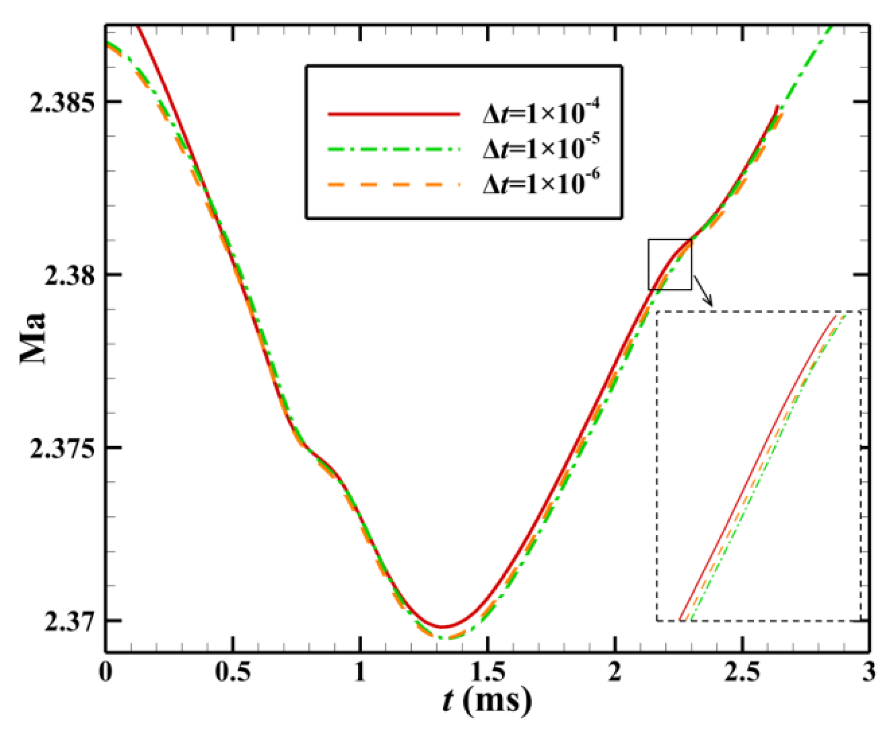
Following the above, unsteady time step (Δt) sensitivity tests were performed to determine the appropriate time step size to achieve efficient and accurate unsteady computation. According to the method in Ref. [33], the preliminary value of the time step is set as 1 × 10⁻⁵. At a Mach number of 3.0, the characteristic velocity was defined as u = Mac (c is the speed of sound), and the dimensionless time step (Δt* = Δt × u/hin) was 3.5 × 10⁻³, indicating that the choice of time step was sufficiently accurate. To further validate the accuracy of the specified time step, three time steps (1 × 10⁻⁴, 1 × 10⁻⁵, and 1 × 10⁻⁶) were chosen for the unsteady numerical simulation verification. Considering the time cost of the calculations, the curve of the Mach number at the exit of the duct at 0–3 ms was calculated for comparative analysis. Figure 5 shows the curves of the Mach number of the exit of the duct at different time steps. It is clear that at time steps of 1 × 10⁻⁴ and 1 × 10⁻⁵, a specific deviation occurred between the curves. However, the curves of the Mach number with time steps of 1 × 10⁻⁵ and 1 × 10⁻⁶ coincided with each other. After calculation, it was found that when ∆t equals 1.0 × 10⁻⁴, 1.0 × 10⁻⁵, and 1.0 × 10⁻⁶, the CFL values are found to be 9.8, 0.98, and 0.098, respectively. Hulme et al. [34] pointed out that low CFL numbers can reduce vibration, reduce numerical diffusion, and improve accuracy. Generally, CFL < 1 and near 1 can be taken so that the accuracy of the numerical solution can be guaranteed while considering the calculation speed and convergence. When ∆t = 1.0 × 10⁻⁵, CFL < 1 and is near 1, thus meeting the requirements. Therefore, it is reasonable to conclude that a time step of 1 × 10⁻⁵ met the needs of the unsteady numerical simulations at the lowest cost.
To measure the impact of the number of nodes of the grid on the results of the calculations, three different sets of grids are used in this paper for numerical simulations under the same conditions of incoming flow: the coarse grid, fine grid, and dense grid contained 8.90 × 10⁶, 1.59 × 10⁷, and 2.39 × 10⁷ cells, respectively. The distributions of velocity in the boundary layer at x/h = 4.1 and the curves of the wall pressure obtained by the simulations with the three sets of grids are shown in Figure 6. Although the densities of the dense and fine grids were different, the simulation results obtained when using them were in good agreement with those obtained with the use of the coarse grid. The fine grid was eventually chosen for subsequent simulations to save time and decrease the cost of calculation.
3.2.2. Numerical Validation
Because the process of the oscillation of dynamic MVGs was simulated based on a dynamic grid, the accuracy of the unsteady numerical simulations combined with the dynamic grid was further verified. The transient numerical simulation of the oscillations and transient pitch of the NACA0012 airfoil were carried out, and the numerical results were compared with those from the experiments [35]. In the experiments, the reference point of the pitch of oscillations of the wing was 0.25 times the chord length, and the oscillation motion is defined by: , where α and ε are the angle of attack and the phase angle depending on the time reference, respectively; α0 is the initial angle of attack; and αm is the amplitude of the angle of attack. The values of αm, α0, and ω were 2.51°, 0.016°, and 392.5, respectively. Figure 7 shows the hysteretical curve of the coefficient of the pitching moment Cm with the angle of attack α, as obtained from numerical simulations of the NACA0012 airfoil. In the figure, it is clear to see that the numerical result was close to the experimental data, and the maximum error between them was no more than ±5%. Therefore, the unsteady numerical simulations with the dynamic grid technique were determined to be adequately accurate.
To validate the predictive capability of the model of turbulence used for vortices induced by the vortex generator, the experimental results of Giepman [36] were selected for testing. The parameters set in the simulation were consistent with the experimental conditions. The Mach number of the incoming flow was Ma = 2.0, and the height of the vortex generator was hv = 8.0 mm. According to the results of 3D particle image velocimetry (PIV) experiments in Ref. [36], the nominal thickness of the boundary layer was δ = 17.5 mm, and the shape factor was H = 2.85 when the vortex generator was not installed. The time-averaged velocity distribution of the boundary layer at this location was obtained from experiments and simulations, as shown in Figure 8a. The characteristics of the distribution of velocity in the downstream wake of the vortex generator need to be measured to assess the control effect. The normal positional distributions of the maximum velocity Vmax and the minimum wake-induced velocity Vmin on the symmetric surface at different flow stations shown in Figure 8b were obtained through the simulations. Figure 8 also shows that the results of Giepman’s experiments and simulations were in good agreement with that of our experiments and simulations. The position of Vmax on the symmetric surface was consistent with the experimental measurements along the direction of the flow, and the maximum difference between the positions was only 0.2hv in the range of hv < x < 27.5hv. The value of Vmin of the wake was within the scope of hv < x < 27.5hv, and the maximum difference between its positions in the experiment and the simulation was only 0.1hv. This shows that the unsteady simulations used in this paper can be used to obtain the complex vortex-induced flow fields within the specific range of the accuracy requirements.
3.2.3. Quasi-Steady Verification
The above method was selected to conduct an unsteady numerical simulation of the flow field induced by a dynamic MVG array to validate the correlation of the flow field between adjacent periods. The frequency of oscillation of the vortex generator was 100 Hz, and the period T is 0.001 s, as shown in Figure 9 (the relative positions of measuring points near the vortex generator are shown in the upper-right part of the figure). The changes in the wall pressure at different monitoring points of the vortex generator over time yielded an interesting phenomenon when t = nT and t = (n + 1) T, whereby the curves of the wall pressure were similar at different measuring points. It can be inferred that the flow field induced by the vortex generator had quasi-stable characteristics; that is, the adjacent periods of oscillation were identical. Thus, the flow in a single period was considered to be representative. To prevent the first period from being affected by the reference flow field, the results of the second period were chosen for data processing.
4. Results and Discussion
4.1. Flow Structure of SWBLI in Supersonic Inlet without Control
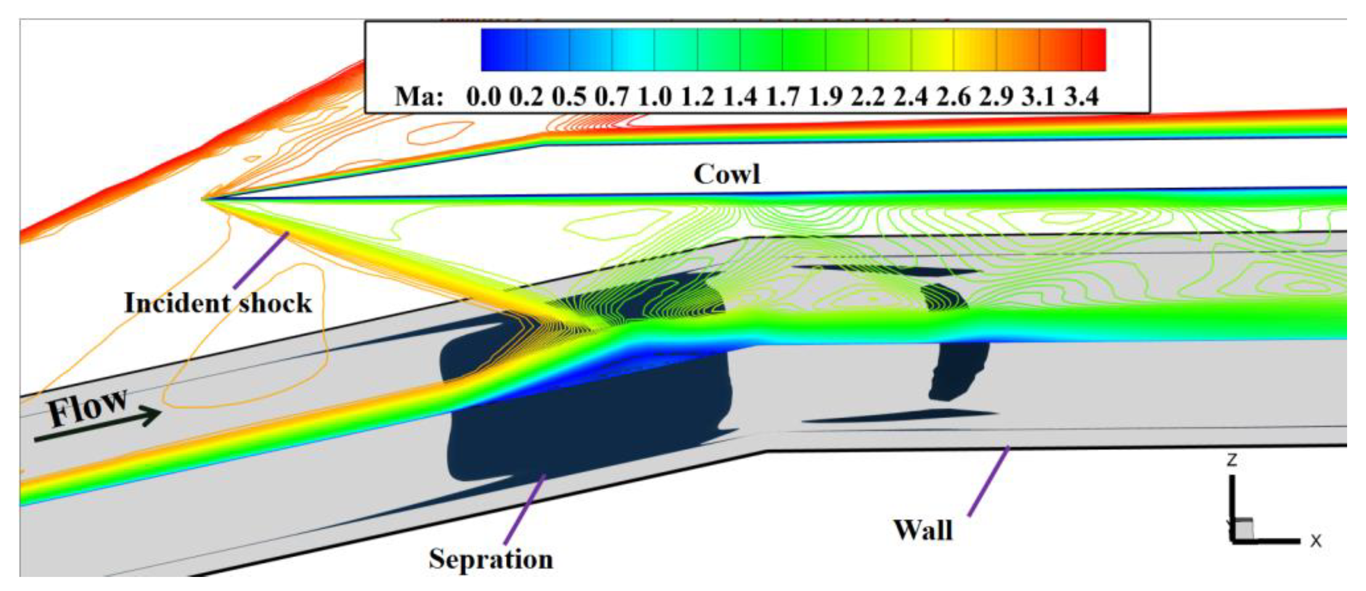
Firstly, the 3D flow inside the inlet without dynamic MVG control was investigated. Figure 10 shows contours of the Mach number on the plane of symmetry of the inlet and the iso-surface of zero velocity at it (the blue curved surface in the figure). The figure shows that the SWBLI led to substantial boundary layer separation at the inlet under this condition, and an extensive range of low-momentum flows were accumulated along the direction of the flow near the side walls, which caused the flow field to exhibit strong three-dimensionality.
Figure 11 shows the boundary layer at different spanwise positions at x/h = 4.7 without flow control (the relative positions are shown in Figure 3). The fullness of the near-wall boundary layer gradually decreased as the distance between it and the side wall decreased. Separation had already occurred in the near-wall boundary layer (y = s + 3.5hv) at x/h = 4.7, indicating that flow was unstable there, and the zone of separation near the side wall was longer than that of the mainstream flow. Figure 12 shows the streamlines emitted 0.05hv from the bottom and side walls of the inlet. Under the incident shock, the vortices generated near the side wall forced the flow toward the center of the channel, and this enhanced the transverse flow near the bottom wall of the inlet.
The spreading slices at different spanwise positions were used for further analysis. The distributions of the Mach number on different slices in the uncontrolled case in Figure 13 shows that the zone of separation gradually became shorter from the plane of symmetry (y = s) to the slice near the side wall. The shape of the separation near the side wall (y = s + 2hv) changed considerably because the glancing interaction between the shock and the boundary layer of the side wall dominated the flow near the latter. It is clear that there was a strong transverse flow at the bottom wall of the inlet. Under its influence, the separated boundary layer was squeezed by the flow of the side wall so that the separation was more significant near the plane of symmetry (y = s).
Figure 14 shows the distributions of the wall limit streamlines on the bottom and side walls of the inlet without flow control. The wall limit streamlines distributions can represent the direction of flow near the wall and reflect the size of the separation area. A pair of prominent corner vortices were generated near each side wall under the action of the incident shock. The size of the separation near the side wall was influenced by this, and the flow field was clearly different from that under the 2D condition. In addition, the boundary layer of the side wall separated upstream of the incident shock. Figure 14b shows that wall limit streamlines also appeared on the side wall, indicating that the interaction between its boundary layer and the incident shock induced large-scale 3D flow separation, leading to the local accumulation of low-energy flow, which had adverse effects on the aerodynamic performance and structural strength of the inlet. Such significant boundary layer separation with complex 3D flow structures and swirling properties negatively impacted the aerodynamic performance of the inlet. Therefore, an effective method of controlling flow is needed to suppress the unfavorable flow induced by the SWBLI and improve the aerodynamic performance of the supersonic inlet.
4.2. Capability of Dynamic MVG Array to Control SWBLI in Supersonic Inlet
4.2.1. Effect of Dynamic MVG Array on Disturbance in Supersonic Boundary Layer
The dynamic array of MVGs was installed to control the SWBLI in the supersonic inlet. The evolution of spatial vortices induced by dynamic vortex generator arrays was investigated first. The vortex structure was represented by a Liutex-Omega isosurface, and the Liutex-R contours of vortex intensity at the five flow stations away from the trailing edge of the vortex generator at different moments were extracted [37]. Figure 15 shows that, at different times, the vortex structures had similar patterns of distribution. Two pairs of vortices were located downstream of the three vortex generators: a main vortex with a more significant range of influence and a secondary vortex below it. The solid black line represents the main vortex’s core line, and the dashed black line represents that of the secondary vortex. The main vortex played a dominant role in the evolution of the downstream flow field, while the secondary vortex had a smaller range of influence and was restricted near the plane of symmetry. According to the contours of the intensities of the vortex at five flow stations at different times, it can be seen that the R values of the Liutex-R of the core positions of the main vortex were relatively high, gradually decreasing around its core. The contours at different times show that each pair of vortices exhibited different changes with the oscillations of the dynamic MVG. As the vortex generator oscillated upward, the radius and intensity of the vortices increased and reached their maximum values at the highest point (t = 1/2T). When the vortex generator swung downward, the radius and intensity of the vortices tended to decrease. Ultimately, a controllable vortex structure was obtained within the supersonic boundary layer.
Moreover, the presence of the SWBLI led to the formation of a strong separation induced vortex in the flow field, as shown in Figure 15. As the vortex generator oscillated upward, the wake-induced vortex penetrated the vortical structure of the SWBLI and weakened it. As the dynamic MVG continued to oscillate, the vortex acting on the region of the SWBLI was further enhanced to make the energy transport more prominent.
Figure 16 shows the time-averaged velocity profiles at the boundary layer at different streamwise positions after the array of dynamic MVGs and includes a schematic diagram of different spanwise positions (shown in the lower-left corner). The velocity u and the distance zn (i.e., the normal distance to the bottom wall of the inlet) were non-dimensionalized by the mainstream velocity u0 and the height of the vortex generator hv. To illustrate the influence of the vortex generator, the velocity distribution at the boundary layer without the vortex generator control is also shown in Figure 16. At the location of x/h = 4.7, the boundary layer velocity distribution at different spanwise positions throughout one cycle is presented. The boundary layer had the same distribution at different spanwise positions except at the plane of symmetry (y = 0hv). The profile of the near-wall boundary layer was relatively thin when the vortex generator was completely embedded into the wall (t = 0T). The profile of the boundary layer became fuller as the vortex generator slowly oscillated upward and became full when it swung to the highest point (t = 1/2T). As the spanwise position gradually moved away from the plane of symmetry y = 0hv, the velocity of the near-wall boundary layer increased on the spanwise plane of y = 0.5hv and further increased at spanwise planes of y = 0.75hv and y = hv. Therefore, the best position for controlling the flow was not on the plane of symmetry y = 0hv but at positions at a certain distance from it. In addition, the near-wall boundary layer at any streamwise position under dynamic MVG control was fuller than that under the uncontrolled condition. This indicates that the array of dynamic MVGs could increase the momentum in the near-wall region and enable the boundary layer to overcome the strong adverse pressure gradient induced by the cowl shock.
Figure 17 shows the distribution of streamlines in the instantaneous flow field around the dynamic MVG to better understand the origin of the wake of the vortex generator. The starting points of the streamlines were located at the leading edge of the dynamic MVG, and the normal heights zn were 10%hv, 2.5%hv, 1%hv, and 0.5%hv. The typical feature of the instantaneous structure of the wake of the dynamic MVGs was a pair of counter-rotating vortices, and this is consistent with the analysis in the previous section. Streamlines from the upstream boundary layer fell off along the side edge of the dynamic MVG and rolled up to form streamwise vortices. Streamwise vortices from both sides eventually merged into the streamwise counter-rotating vortex pair at the rear of the dynamic MVG. Some of the streamlines emitted from the upstream boundary layer at the normal height of zn = 10%hv bypassed the flow of the dynamic MVG and did not directly enter the wake, indicating that a lower volume of the fluid was entrained inside the vortex at this height. The streamlines emitted below zn = 10%hv constituted the wake of the dynamic MVG, and their final position was close to the core of the vortex, especially near the wall. In summary, the dynamic MVG induced a pair of streamwise vortices in supersonic flow that gathered low-momentum flow from the bottom layer of the boundary layer on both sides toward the centerline and lifted it upward. Meanwhile, the high-momentum flow above the boundary layer was entrained by the streamwise vortices and mixed with the flow inside the boundary layer to help achieve the objective of control.
The above analysis indicates that the vortex generator has a unique collection function for the near-wall boundary layer. It is clear from the distribution of streamlines around the dynamic MVG shown in Figure 18 that although, when it swung down to t = 3/4T, the height of the vortex generator was the same as that at t = 1/4T, the airflow below it was extruded by its trailing edge at t = 3/4T, while only prominent suction was observed at t = 1/4T. When the vortex generator swung upward, air flowed into the cavity below it from both sides. The typical profile of the velocity of the boundary layer at the position shown in Figure 19 indicates a significant increase in the near-wall velocity at t = 3/4T compared with that at t = 1/4T, indicating that the unique “extrusion” and “suction” functions of the dynamic MVG continued to charge the airflow.
4.2.2. Effect of Dynamic MVG Array on SWBLI
The above analysis indicates that the dynamic MVG can induce vortices of controllable strength and significantly change the fullness of the boundary layer under conditions of supersonic inflow. Subsequently, a control characteristics analysis was conducted to examine its influence on the SWBLI region of the supersonic inlet. Figure 20 shows the time-averaged contours of the Mach number on different spanwise planes under the control of the array of MVGs. Compared with the case without control, the low-momentum region near the wall decreased at all spanwise positions under dynamic MVG-based control. The separation bubble gradually decreased in size from the plane of symmetry of the vortex generator to the other spanwise positions because the planes y = 0hv and y = s were in the middle of the streamwise vortices induced by the vortex generator, and mixing had a minor effect on it. The planes of y = 0.5hv, y = 0.75hv, y = s + 0.5hv, and y = s + 0.75hv were located in the streamwise vortices induced by the trailing edge of the vortex generator. The mixing resulting from the streamwise vortices was strong and reduced the size of the separation bubble.
Figure 21 shows the distributions of the time-averaged static pressure and wall friction coefficient cf along the wall. The method proposed by Kendall and Koochesfahani [38] was used to estimate the friction velocity uτ. The wall shear stress τw can be calculated using the relation . The wall friction coefficient was . Increasing the local cf value can delay the separation and reduce the disturbance area at the same time. Therefore, the cf value reflects the flow field characteristics and control effect of the SWBLI [39]. The solid lines represent the time-averaged wall static pressure, and the dashed lines represent the distribution of cf on the wall. The static pressure on the wall at different spanwise positions in the separation when the array of dynamic MVGs was used was significantly lower than in the uncontrolled flow field, indicating that the array could reduce local high pressure near the separation. The distribution of cf of the wall on the corresponding xoz plane showed that the uncontrolled state had a shear stress on the wall opposite to the flow direction in the separation (x/h = 5.30~x/h = 7.00). The velocity gradient was negative, which is highly unfavorable for the efficiency of the inlet. However, the reverse shear stress at each spanwise position was reduced in the case involving control. The effects on the shear stress in the separation at y = 0.5hv (x/h = 5.65~x/h = 6.81) and y = 0.75hv (x/h = 5.61~x/h = 6.92) were better with control than without it. The length of the separation could be reduced by up to 31.76% compared with the uncontrolled case. However, the plane of symmetry y = 0hv was located in an area in which the two inner vortices interfered with each other, and the control effect was not as good as that at the other spanwise planes, which is consistent with the above discussion on the distribution of the time-averaged Mach number. In summary, the array of dynamic MVGs was able to reduce local high pressure near the separation and improve the downstream cf of the wall.
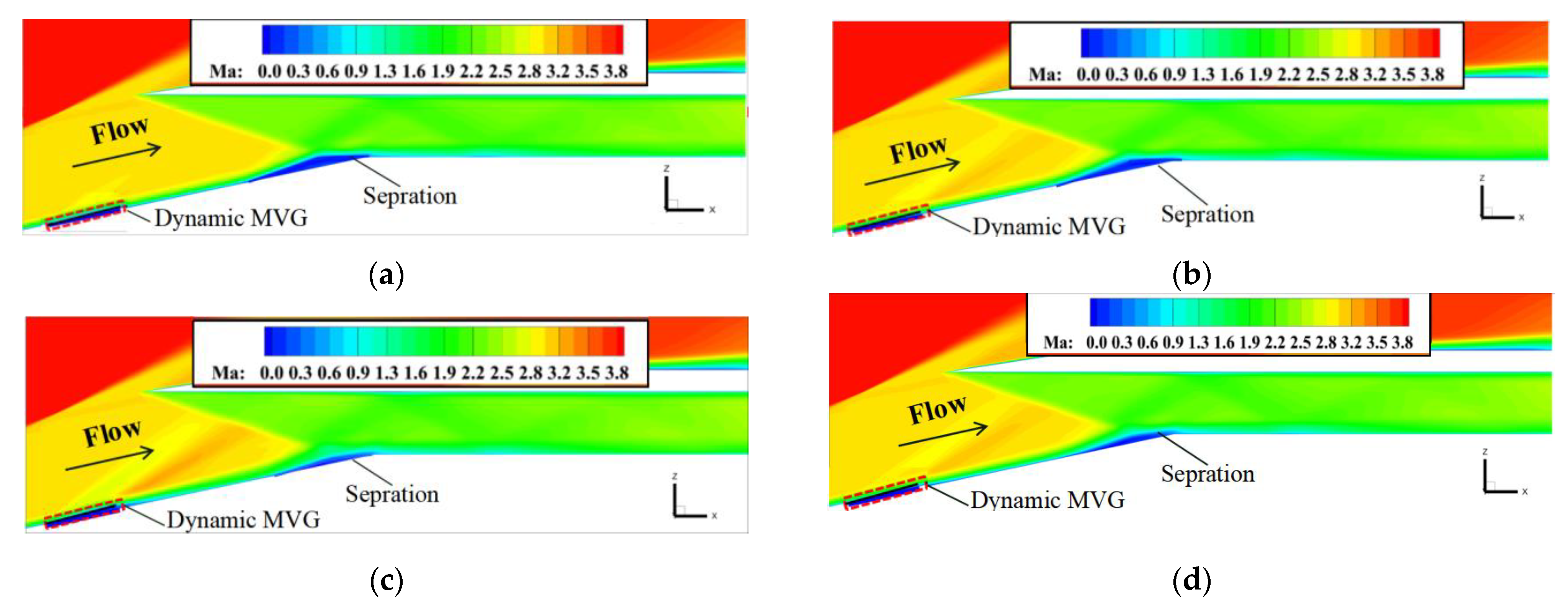
To verify the control characteristics of the vortex generator at different times, an instantaneous Mach number contour was extracted at the position of y = 0.25hv at t = 0T, t = 1/4T, t = 1/2T, and t = 3/4T. Figure 22 shows that the size of the separation bubble decreased as the vortex generator swung upward. When it swung to the highest point at t = 1/2T, the separated boundary layer quickly reattached, and the control effect was better than at other times. This is because the scale and strength of the vortex peaked when the vortex generator swung to the highest point (t = 1/2T), as discussed above. When it swung downward, the separation bubble continued to decrease in size due to the “extrusion” effect of the dynamic MVGs.
Figure 23 shows the distributions of the shear stress and limit streamlines on the wall at different times when controlled by the array of MVGs. Figure 23 shows that as the array of dynamic MVGs oscillated, the size of the separation bubble varied. The improvement in the shear stress on the wall on the plane of symmetry was better at t = 1/2T and t = 3/4T. Under the control of the array of MVGs, the corner vortices disappeared, and the corner separation decreased. The separation line gradually formed a sawtooth shape, leading to a significant difference in the length of the separation at different spanwise positions. The separation near the y = 0hv plane had the shortest flow, and the control effect at the y = ±s/2 planes was not as good as the other spanwise planes because they were located between the trailing vortices of the array of vortex generators. In conclusion, the dynamic MVGs could satisfactorily control the interaction between the shock and the boundary layer. Compared with that in the absence of control, the length of flow in the separation region was significantly reduced, and the total pressure recovery coefficient increased by 6.4%.
4.3. Influence of Dynamic Frequency of MVG Array on its Control Effect
Figure 24 shows variations in the shape factor and contours of the time-averaged Mach number on the plane y = 0.25hv under different frequencies. The variations in the shape factor H are shown in Figure 24a. The kinetic energy loss caused by viscosity is closely related to the fullness of the velocity profile in the boundary layer; the shape factor was introduced to express the relative kinetic energy loss in the boundary layer. The smaller the H, the fuller the boundary layer [40]. The monitoring position (dashed black line on the plane of symmetry y = 0.25hv in Figure 24b) was located upstream of the separation bubble at x/h = 5.4. Considering the limits imposed by the speed of the motor and the feasibility of the structure, the frequency of oscillations f of the vortex generator was controlled to within 300 Hz, and three frequencies (f1 = 50 Hz, f2 = 150 Hz, and f3 = 300 Hz) were selected for analysis. Figure 24 shows that H decreased for 3/4T as the duration of oscillations increased, indicating that the vortex generator had enhanced the exchange of energy between the boundary layer and the mainstream, increased the fullness of the near-wall boundary layer, and was expected to achieve flow control. When the vortex generator oscillated at f3, the value of the shape factor H at each instance was smaller than those at f1 and f2, and the maximum reduction reached 30%. This indicates that as the oscillation frequency of the dynamic MVGs increased, the frequencies of “suction” and “extrusion” of the airflow increased, leading to a higher intensity of energy transfer to airflow and a more significant effect in flow control. As can be seen from the time-averaged Mach number contour in Figure 24b, the height and length of the separation bubble decrease with the increase in the vortex generator’s oscillation frequency, and this is because a higher oscillation frequency leads to more momentum injection into the near-wall region, which helps to overcome the adverse pressure gradient caused by SWBLI. This reduces the size of the separation bubble, which is consistent with the control effect of the shape factor change mentioned earlier.
Figure 25a shows the profiles of velocity near the wall (zn/hv < 0.2) at the streamwise position x/h = 4.7 (x = 70 mm) and the spanwise positions y = 0.25hv and y = 0.75hv. As the frequency of oscillation increased, the profile of the boundary layer near the wall at both spanwise positions gradually became fuller. However, compared with those at y = 0.25hv, the changes in the near-wall velocity were more pronounced at the spanwise position of y = 0.75hv. When the MVG oscillated at a frequency of 300 Hz, the profile of the boundary layer was the fullest, and the near-wall velocity could be increased by up to 8.8% compared with that at f1 = 50 Hz. The vortex generator had the most significant control effect on the flow field at a frequency of 300 Hz. In addition, Figure 25b shows the profiles of velocity near the wall at the streamwise positions of x/h = 4.1 and x/h = 4.7 (spanwise position, y = 0.5hv). When the dynamic MVG oscillated at a frequency of 300 Hz, the near-wall velocity increased to varying degrees at both streamwise positions, with more significant changes observed at x/h = 4.7. In summary, when the frequency of oscillations of the dynamic MVG increased, the near-wall boundary layer at each station obtained more kinetic energy, and this led to a more pronounced control effect.
5. Conclusions
In this study, we proposed a method for controlling the SWBLI in a supersonic inlet by using an array of dynamic MVGs. The aerodynamic feasibility of this design concept was preliminarily verified, and the mechanism of flow and the law of influence of the relevant parameters were analyzed. Our main conclusions are as follows:
- (1)
- The incident shock in the supersonic inlet imposed a strong adverse pressure gradient on the boundary layer, which led to its local thickening and separation. Due to the presence of the side wall of the inlet, vortices that intensified transverse flow were generated near the side wall, leading to a complex 3D structure of flow of the separation bubble. A large separation was formed in the middle of the bottom wall.
- (2)
- The dynamic MVGs induced a vortex structure with variable intensity in the supersonic boundary layer due to their oscillation. This enhanced the mixing of the flow of the boundary layer with the high-speed mainstream flow and caused the profile of the velocity of the separation to become fuller while enhancing the stability of the boundary layer. At the same time, the unique effects of “extrusion” and “suction” of the vortex generators during their oscillation continued to charge the airflow, further enhancing its ability to suppress the separation.
- (3)
- When flow was controlled by the array of dynamic MVGs, the height of the separation bubble in the supersonic inlet decreased more significantly than that in the absence of control. Compared with the case without control, the length of the separation in the streamwise direction decreased by up to 31.76%, and the coefficient of total pressure recovery increased by 6.4%.
- (4)
- When the frequency of the dynamic MVG was in the range of 50–300 Hz, the effect of charging the low-speed airflow near the boundary layer was enhanced as the frequency of oscillations of the vortex generators increased, and the shape factor of the boundary layer decreased by up to 30% at a frequency of 300 Hz compared with that in the absence of control.
Author Contributions
Conceptualization, Y.Z. and M.W.; methodology, M.W., Z.W. and H.T.; validation, M.W. and Y.Z.; formal analysis, M.W.; investigation, M.W.; resources, Y.Z.; data curation, Y.Z. and Z.W.; writing—original draft preparation, M.W.; writing—review and editing, Y.Z., Z.W., D.C., K.W. and S.G.; visualization, K.W. and D.C.; supervision, Y.Z. and Z.W.; project administration, Y.Z.; funding acquisition, Y.Z. All authors have read and agreed to the published version of the manuscript.
Funding
This work was funded by the National Natural Science Foundation of China (Grant Nos. 12025202, 12172175), the Postgraduate Research & Practice Innovation Program of NUAA (Grant No. xcxjh20220203), the Open Fund from Laboratory of Aerodynamics in Multiple Flow Regimes (Grant No. KLYSYS-KFJJ-ZD-2022-02), and the Young Scientific and technological Talents Project of Jiangsu Association for Science and Technology (Grant No. TJ-2021-052).
Institutional Review Board Statement
Not applicable.
Informed Consent Statement
Written informed consent has been obtained from the patient(s) to publish this paper.
Data Availability Statement
The data within the article can be made available upon request.
Conflicts of Interest
The authors declare that they have no known competing financial interests or personal relationships that could have appeared to influence the work reported in this paper.
References
- Seddon, J.; Goldsmith, E.L. Intake Aerodynamics; AIAA Education Series; American Institute of Aeronautics and Astronautics: New York, NY, USA, 1985; pp. 1–30. [Google Scholar]
- Holden, M. Historical review of experimental studies and prediction methods to describe laminar and turbulent shock wave/boundary layer interactions in hypersonic flows. In Proceedings of the 44th AIAA Aerospace Sciences Meeting and Exhibit, Reno, NV, USA, 9–12 January 2006. [Google Scholar]
- Tan, H.-J.; Li, C.-H.; Zhang, Y.; Li, G.-S. Review of progress in shock control technology with fixed geometry. J. Propul. Technol. 2016, 37, 2001–2008. [Google Scholar]
- Van Wie, D.M. Scramjet inlets. In Scramjet Propulsion; Curran, E.T., Murthy, S.N.B., Eds.; American Institute of Aeronautics and Astronautics: Reston, VA, USA, 2000; Volume 189, pp. 447–511. [Google Scholar]
- Pan, H.-L.; Li, J.-H.; Shen, Q. Studies of turbulence/shock interaction in a scramjet inlet. J. Propul. Technol. 2013, 34, 1172–1178. [Google Scholar]
- Yuan, H.C.; Liang, D.W. Effect of suction on starting of hypersonic inlet. J. Propul. Technol. 2006, 27, 525–528. [Google Scholar]
- Yan, H.-M.; Zhong, J.-J.; Han, J.-A.; Feng, Z.-M. Research on boundary layer suction in the throat of supersonic inlet. J. Propul. Technol. 2009, 30, 175–181. [Google Scholar]
- Zhao, J.; Fan, X.-Q.; Wang, Y.; Tao, J. Classification of flow field in supersonic boundary layer bleed slot. J. Propul. Technol. 2017, 38, 2463–2470. [Google Scholar]
- Shi, X.; Lyu, M.; Zhao, Y.; Tao, S.; Hao, L.; Yuan, X. Flow control technique for shock wave/turbulent boundary layer interactions. Acta Aeronaut. Astronaut. Sin. 2022, 43, 625929. [Google Scholar]
- Wu, H.; Wang, J.; Huang, W.; Du, Z.; Yan, L. Research progress on shock wave/boundary layer interactions and flow controls induced by micro vortex generators. Acta Aeronaut. Astronaut. Sin. 2021, 42, 25371. [Google Scholar]
- Babinsky, H.; Li, Y.; Pitt Ford, C.W. Microramp control of supersonic oblique shock-wave/boundary-layer interactions. AIAA J. 2009, 47, 668–675. [Google Scholar] [CrossRef]
- Wang, B.; Liu, W.; Zhao, Y.; Fan, X.; Wang, C. Experimental investigation of the microramp based shock wave and turbulent boundary layer interaction control. Phys. Fluids 2012, 24, 055110. [Google Scholar]
- Blinde, P.L.; Humble, R.A.; van Oudheusden, B.W.; Scarano, F. Effects of micro-ramps on a shock wave/turbulent boundary layer interaction. Shock Waves 2009, 19, 507–520. [Google Scholar] [CrossRef]
- Anderson, B.H.; Tinapple, J.; Surber, L. Optimal control of shock wave turbulent boundary layer interactions using micro-array actuation. In Proceedings of the 3rd AIAA Flow Control Conference, San Francisco, CA, USA, 5–8 June 2006. [Google Scholar]
- Zhang, Y.; Tan, H.-J.; Du, M.-C.; Wang, D.-P. Control of shock/boundary-layer interaction for hypersonic inlets by highly swept microramps. J. Propul. Power 2015, 31, 133–143. [Google Scholar] [CrossRef]
- Anderson, B.H.; Mace, J.L.; Mani, M. Active “fail safe” micro-array flow control for advanced embedded propulsion systems. In Proceedings of the 47th Aerospace Sciences Meeting, sponsored by the American Institute of Aeronautics and Astronautics, Orlando, FL, USA, 5–8 January 2009. [Google Scholar]
- Wagner, J.L. Experimental Studies of Unstart Dynamics in Inlet/Isolator Configurations in a Mach 5 Flow. Ph.D. Thesis, The University of Texas at Austin, Austin, TX, USA, 2009. [Google Scholar]
- Giepman, R.H.M.; Schrijer, F.F.J.; Van Oudheusden, B.W. Flow control of an oblique shock wave reflection with micro-ramp vortex generators: Effects of location and size. Phys. Fluids 2014, 26, 066101. [Google Scholar] [CrossRef]
- Wang, M.G.; He, X.M.; Wang, J.J.; Zhang, Y.; Wang, K.; Tan, H.J.; Li, L.G. Shock wave/boundary layer interaction control method based on oscillating vortex generator. J. Aviat. 2023, 1–16. Available online: http://kns.cnki.net/kcms/detail/11.1929.v.20230421.1348.010.html (accessed on 14 August 2023).
- Lee, S.; Goettke, M.K.; Loth, E.; Tinapple, J.; Benek, J. Microramps upstream of an oblique-shock/boundary-layer interaction. AIAA J. 2010, 48, 104–118. [Google Scholar] [CrossRef]
- Van Leer, B. Towards the ultimate conservative difference scheme. V. A second-order sequel to Godunov’s method. J. Comput. Phys. 1979, 32, 101–136. [Google Scholar] [CrossRef]
- White, F.M. Viscous Fluid Flow; McGraw-Hill: New York, NY, USA, 1991. [Google Scholar]
- Jiao, X.; Chang, J.; Wang, Z.; Yu, D. Numerical study on hypersonic nozzleinlet starting characteristics in a shock tunnel. Acta Astronaut. 2017, 130, 167–179. [Google Scholar] [CrossRef]
- Sekar, K.R.; Karthick, S.K.; Jegadheeswaran, S.; Kannan, R. On the unsteady throttling dynamics and scaling analysis in a typical hypersonic inlet–isolator flow. Phys. Fluids 2020, 32, 126104. [Google Scholar] [CrossRef]
- Huang, H.-X.; Tan, H.-J.; Sun, S.; Ling, Y. Evolution of supersonic corner vortex in a hypersonic inlet/isolator model. Phys. Fluids 2016, 28, 126101. [Google Scholar] [CrossRef]
- Jiao, X.; Chang, J.; Wang, Z.; Yu, D. Mechanism study on local unstart of hypersonic inlet at high Mach number. AIAA J. 2015, 53, 3102–3112. [Google Scholar] [CrossRef]
- Menter, F.R. Two-equation eddy-viscosity turbulence models for engineering applications. AIAA J. 1994, 32, 1598–1605. [Google Scholar] [CrossRef]
- ANSYS Inc. Fluent Theory Guide; ANSYS Inc.: Canonsburg, PA, USA, 2018. [Google Scholar]
- Wilcox, D.C. Turbulence Modeling for CFD; DCW Industries: La Cañada, CA, USA, 1993. [Google Scholar]
- Li, N.; Chang, J.T.; Xu, K.J.; Yu, D.R.; Bao, W.; Song, Y.P. Prediction dynamic model of shock train with complex background waves. Phys. Fluids 2017, 29, 116103. [Google Scholar] [CrossRef]
- Jordan, C.; Edwards, J.R.; Stefanski, D.L. Evaluation of RANS closure models using LES datasets for hypersonic shock boundary layer interactions. In Proceedings of the AIAA Scitech 2021 Forum, Virtual, 11–15 January 2021. [Google Scholar]
- Bonne, N.; Brion, V.; Garnier, E.; Bur, R.; Molton, P.; Sipp, D.; Jacquin, L. Analysis of the two-dimensional dynamics of a Mach 1.6 shock wave/transitional boundary layer interaction using a RANS based resolvent approach. J. Fluid Mech. 2019, 862, 1166–1202. [Google Scholar] [CrossRef]
- Hong, W.; Kim, C. Computational study on hysteretic inlet buzz characteristics under varying mass flow conditions. AIAA J. 2014, 52, 1357–1373. [Google Scholar] [CrossRef]
- Hulme, I.; Clavelle, E.; Van der Lee, L.; Kantzas, A. CFD Modeling and Validation of Bubble Properties for a Bubbling Fluidized Bed. Ind. Eng. Chem. Res. 2005, 44, 4254–4266. [Google Scholar] [CrossRef]
- Lambourne, N.C.; Landon, R.H.; Zwaan, R.J. Compendium of Unsteady Aerodynamics Measurements; AGARD-R-702; Technical Editing and Reproduction Ltd.: London, UK, 1982. [Google Scholar]
- Giepman, R.; Srivastava, A.; Schrijer, F.; van Oudheusden, B. The effects of Mach and Reynolds number on the flow mixing properties of micro-ramp vortex generators in a supersonic boundary layer. In Proceedings of the 45th AIAA Fluid Dynamics Conference, Dallas, TX, USA, 22–26 June 2015. [Google Scholar]
- Liu, C.Q. Liutex-vortex definition and the third generation vortex recognition method. Acta Aerodyn. Sin. 2020, 38, 413–431. [Google Scholar]
- Kendall, A.; Koochesfahani, M. A method for estimating wall friction in turbulent wall-bounded flows. Exp. Fluids 2008, 44, 773–780. [Google Scholar] [CrossRef]
- Babinsky, H.; Titchener, N. Shock Boundary Layer Interaction Flow Control with Micro Vortex Generators; European Office of Aerospace Research and Development: London, UK, 2011. [Google Scholar]
- Babinsky, H.; Harvey, J.K. Shock Wave–Boundary-Layer Interactions; Cambridge University Press: Cambridge, UK, 2011. [Google Scholar]
Figure 1.
Design concept of the dynamic MVG. (a) Flat state of the dynamic MVG. (b) Oscillating state of the dynamic MVG.
Figure 1.
Design concept of the dynamic MVG. (a) Flat state of the dynamic MVG. (b) Oscillating state of the dynamic MVG.

Figure 2.
Schematic diagram of the proposed model. (a) Schematic diagram of the configuration of the inlet. (b) Structure of the dynamic MVG.
Figure 2.
Schematic diagram of the proposed model. (a) Schematic diagram of the configuration of the inlet. (b) Structure of the dynamic MVG.

Figure 3.
Relative positions of the array of dynamic MVGs.

Figure 4.
Grid topology of the array of dynamic MVGs.

Figure 5.
Curves of the Mach number at the exit of the duct with timesteps of different sizes.

Figure 6.
Profile of the boundary layer and distribution of the wall pressure with grids of different sizes. (a) Distributions of velocity at the boundary layer (x/h = 4.1) with grids of different sizes. (b) Wall pressure with grids of different sizes.
Figure 6.
Profile of the boundary layer and distribution of the wall pressure with grids of different sizes. (a) Distributions of velocity at the boundary layer (x/h = 4.1) with grids of different sizes. (b) Wall pressure with grids of different sizes.

Figure 7.
Comparison between the coefficients of the pitching moment obtained from experiments and simulations.
Figure 7.
Comparison between the coefficients of the pitching moment obtained from experiments and simulations.

Figure 8.
Comparison between the results of experiments and simulations. (a) Comparison of the velocity distribution of the boundary layer between the experiment and the simulation [36]. (b) The points of the highest and lowest velocities of the wake on a plane of symmetry [36].

Figure 9.
Variations in pressure at typical measuring points near the dynamic MVG over time.

Figure 10.
Contours of the Mach number on the planes of symmetry and zero velocity of the inlet without flow control.
Figure 10.
Contours of the Mach number on the planes of symmetry and zero velocity of the inlet without flow control.

Figure 11.
Boundary layer at different spanwise positions at x/h = 4.7 without control.

Figure 12.
Streamlines emanating from the bottom and side walls at 0.05hv.

Figure 13.
Distributions of the Mach number in different xoz planes without control.

Figure 14.
Distributions of wall limit streamlines on the bottom and side walls of the duct without control. (a) Streamlines emitted 0.05hv from the bottom and side walls of the duct. (b) Distributions of the wall limit streamlines on the side walls.
Figure 14.
Distributions of wall limit streamlines on the bottom and side walls of the duct without control. (a) Streamlines emitted 0.05hv from the bottom and side walls of the duct. (b) Distributions of the wall limit streamlines on the side walls.

Figure 15.
Evolution of the vortex along the direction of flow of the array of dynamic MVG. (a) t = 0T. (b) t = 1/4T. (c) t = 2/4T. (d) t = 3/4T.
Figure 15.
Evolution of the vortex along the direction of flow of the array of dynamic MVG. (a) t = 0T. (b) t = 1/4T. (c) t = 2/4T. (d) t = 3/4T.

Figure 16.
Profiles of the boundary layer at different spanwise positions at x/h = 4.7 at five typical times within one cycle. (a) y = 0hv. (b) y = 0.5hv. (c) y = 0.75hv. (d) y = hv.
Figure 16.
Profiles of the boundary layer at different spanwise positions at x/h = 4.7 at five typical times within one cycle. (a) y = 0hv. (b) y = 0.5hv. (c) y = 0.75hv. (d) y = hv.

Figure 17.
Distribution of streamlines around the array of dynamic MVGs in an instantaneous flow field. (a) zn = 10%hv. (b) zn = 2.5%hv. (c) zn = 1.0%hv. (d) zn = 0.5%hv.
Figure 17.
Distribution of streamlines around the array of dynamic MVGs in an instantaneous flow field. (a) zn = 10%hv. (b) zn = 2.5%hv. (c) zn = 1.0%hv. (d) zn = 0.5%hv.

Figure 18.
Distribution of streamlines around the dynamic MVG. (a) t = 1/4T. (b) t = 3/4T.

Figure 19.
Profiles of velocity at x/h = 4.7 during “suction” and “extrusion” (the solid lines represent “suction”, and the dashed lines represent “extrusion”).
Figure 19.
Profiles of velocity at x/h = 4.7 during “suction” and “extrusion” (the solid lines represent “suction”, and the dashed lines represent “extrusion”).

Figure 20.
Time-averaged Mach number of the vortex generator at different spanwise positions.

Figure 21.
Distributions of the time−averaged parameters of the array of dynamic MVGs in different xoz planes. (a) Distribution of the time-averaged static pressure along the wall. (b) Distribution of the time−averaged wall friction coefficient along the wall.
Figure 21.
Distributions of the time−averaged parameters of the array of dynamic MVGs in different xoz planes. (a) Distribution of the time-averaged static pressure along the wall. (b) Distribution of the time−averaged wall friction coefficient along the wall.

Figure 22.
Contours of the Mach number of the array of dynamic MVGs at different times: (a) t = 0T, (b) t = 1/4T, (c) t = 1/2T, (d) t = 3/4T.
Figure 22.
Contours of the Mach number of the array of dynamic MVGs at different times: (a) t = 0T, (b) t = 1/4T, (c) t = 1/2T, (d) t = 3/4T.

Figure 23.
The distributions of the shear stress and limit streamlines on the wall at different times: (a) t = 0T, (b) t = 1/4T, (c) t = 2/4T, (d) t = 3/4T.
Figure 23.
The distributions of the shear stress and limit streamlines on the wall at different times: (a) t = 0T, (b) t = 1/4T, (c) t = 2/4T, (d) t = 3/4T.


Figure 24.
Contours of the mean Mach number and changes in the shape factor at different frequencies of oscillation at y = 0.25hv. (a) Changes in the H at different times. (b) Changes in the contour of the mean Mach number.
Figure 24.
Contours of the mean Mach number and changes in the shape factor at different frequencies of oscillation at y = 0.25hv. (a) Changes in the H at different times. (b) Changes in the contour of the mean Mach number.

Figure 25.
Changes in velocity at different frequencies of oscillation. (a) Velocity distributions at different spanwise positions (x/h = 4.7). (b) Velocity distributions at different streamwise positions (y = 0.5hv).
Figure 25.
Changes in velocity at different frequencies of oscillation. (a) Velocity distributions at different spanwise positions (x/h = 4.7). (b) Velocity distributions at different streamwise positions (y = 0.5hv).


Table 1.
Main design parameters of the model and the dynamic MVG.
| Design Parameter | Value |
|---|---|
| h (mm) | 14.4 |
| hv (mm) | 4.0 |
| hin (mm) | 24.9 |
| W (mm) | 110.0 |
| AP | 24.0 |
| s (mm) | 30.0 |
| c (mm) | 28.8 |
| α (°) | 12.0 |
| Xp (mm) | 40 |
Disclaimer/Publisher’s Note: The statements, opinions and data contained in all publications are solely those of the individual author(s) and contributor(s) and not of MDPI and/or the editor(s). MDPI and/or the editor(s) disclaim responsibility for any injury to people or property resulting from any ideas, methods, instructions or products referred to in the content. |
© 2023 by the authors. Licensee MDPI, Basel, Switzerland. This article is an open access article distributed under the terms and conditions of the Creative Commons Attribution (CC BY) license (https://creativecommons.org/licenses/by/4.0/).
Share and Cite
MDPI and ACS Style
Wang, M.; Wang, Z.; Zhang, Y.; Cheng, D.; Tan, H.; Wang, K.; Gao, S. Control of Cowl Shock/Boundary Layer Interaction in Supersonic Inlet Based on Dynamic Vortex Generator. Aerospace 2023, 10, 729. https://doi.org/10.3390/aerospace10080729
AMA Style
Wang M, Wang Z, Zhang Y, Cheng D, Tan H, Wang K, Gao S. Control of Cowl Shock/Boundary Layer Interaction in Supersonic Inlet Based on Dynamic Vortex Generator. Aerospace. 2023; 10(8):729. https://doi.org/10.3390/aerospace10080729
Chicago/Turabian StyleWang, Mengge, Ziyun Wang, Yue Zhang, Daishu Cheng, Huijun Tan, Kun Wang, and Simin Gao. 2023. "Control of Cowl Shock/Boundary Layer Interaction in Supersonic Inlet Based on Dynamic Vortex Generator" Aerospace 10, no. 8: 729. https://doi.org/10.3390/aerospace10080729
Note that from the first issue of 2016, this journal uses article numbers instead of page numbers. See further details here.